A Method to Identify the Boundary Between Rocky and Gaseous Exoplanets from Tidal Theory and Transit Durations

Abstract

The determination of an exoplanet as rocky is critical for the assessment of planetary habitability. Observationally, the number of small-radius, transiting planets with accompanying mass measurements is insufficient for a robust determination of the transitional mass or radius. Theoretically, models predict that rocky planets can grow large enough to become gas giants when they reach $\sim 10~{}{\rm\,M_{Earth}}$, but the transitional mass remains unknown. Here I show how transit data, interpreted in the context of tidal theory, can reveal the critical radius that separates rocky and gaseous exoplanets. Standard tidal models predict that rocky exoplanets’ orbits are tidally circularized much more rapidly than gaseous bodies’, suggesting the former will tend to be found on circular orbits at larger semi-major axes than the latter. Well-sampled transits can provide a minimum eccentricity of the orbit, allowing a measurement of this differential circularization. I show that this effect should be present in the data from the Kepler spacecraft, but is not apparent. Instead, it appears that there is no evidence of tidal circularization at any planetary radius, probably because the publicly-available data, particularly the impact parameters, are not accurate enough. I also review the bias in the transit duration toward values that are smaller than that of planets on circular orbits, stressing that the azimuthal velocity of the planet determines the transit duration. The ensemble of Kepler planet candidates may be able to determine the critical radius between rocky and gaseous exoplanets, tidal dissipation as a function of planetary radius, and discriminate between tidal models.

1. Introduction

Planetary habitability is a complex function of orbits, composition, atmospheric evolution and geophysical processes. Most searches for habitable environments begin with the comparison of a planet’s orbit relative to the host star’s habitable zone (HZ), the region around a star for which an Earth-like planet can support water on its surface (Dole, 1964; Kasting et al., 1993; Selsis et al., 2007; Kopparapu et al., 2013). A critical feature of this definition is the presence of a solid surface, i.e. the planet must be rocky. Hence, this determination is also crucial in the identification of potentially habitable environments.

Unfortunately a robust and universal definition of the boundary between rocky and gaseous worlds has remained elusive. Initially, research was theoretical and identified the mass of a solid body, a “core,” that was large enough to permit the capture of protoplanetary gas (e.g.  Pollack et al., 1996; Ikoma et al., 2001; Hubickyj et al., 2005; Guillot, 2005; Militzer et al., 2008; Lissauer et al., 2009; Movshovitz et al., 2010). These results showed that a wide range of “critical masses” are possible, from $~{}\hbox to0.0pt{$<$\hss}{\lower 4.30554pt\hbox{$\sim$}}1-20~{}{\rm\,M_{Earth}}$. Undoubtedly, the actual critical mass is a function of the local protoplanetary disk’s properties (e.g. temperature and viscosity), and one should expect the critical mass to vary from system to system. However, there should exist a maximum mass (or radius) below which planets are terrestrial-like because small mass planets do not possess enough gravitational force to hold on to hydrogen and helium. In this study, I examine the possibility that this boundary can be identified with transit data coupled with expectations from tidal theory.

Transiting exoplanets offer the opportunity to measure both the planetary radius and mass. The planetary radius can be constrained if the stellar radius is known, usually determined from spectral information (Torres et al., 2010; Everett et al., 2013), but sometimes directly through interferometric observations (von Braun et al., 2011; Boyajian et al., 2012). The mass can then be measured through radial velocity measurements, which no longer suffer from the mass-inclination degeneracy as the viewing geometry is known (e.g.  Batalha et al., 2011). Recently, Mislis et al. (2012) demonstrated that Kepler light curves can reveal the mass of a close-in and massive planets via ellipsoidal variations. In multiple planet systems, masses can also be measured by transit timing variations (Agol et al., 2005; Holman & Murray, 2005), as for Kepler-9 (Holman et al., 2010) and Kepler-11 (Lissauer et al., 2011). However, for many transiting planets, these methods may not be available, as terrestrial planets tend to produce small radial velocity and timing variation signals. Thus, direct measurements of the masses of small planets orbiting FGK stars (0.7 – $1.4~{}{\rm\,M_{Sun}}$) will be challenging.

The transit detection method is biased toward the discovery of planets on close-in orbits, $~{}\hbox to0.0pt{$<$\hss}{\lower 4.30554pt\hbox{$\sim$}}0.1$ AU for FGK stars. NASA’s Kepler spacecraft has detected over 1000 planet candidates in this range, opening up the possibility that statistical analyses of these (uninhabitable) planets could reveal the critical radius between terrestrial and gaseous planets, $R_{crit}$. As theoretical models of planet formation have found that the critical mass and radius lies near $10~{}{\rm\,M_{Earth}}$ and $2~{}{\rm\,R_{Earth}}$, planets that are smaller could be rocky. Although few data points exist, it does appear that $R_{crit}<2~{}{\rm\,R_{Earth}}$, e.g. Kepler-10 b with mass $M_{p}=4.56~{}{\rm\,M_{Earth}}$ and radius $R_{p}=1.42~{}{\rm\,R_{Earth}}$ (Batalha et al., 2011) and CoRoT-7 b with $M_{p}<8~{}{\rm\,M_{Earth}}$ and $R_{p}=1.58~{}{\rm\,R_{Earth}}$ (Léger et al., 2009; Queloz et al., 2009; Ferraz-Mello et al., 2011). Here I will call rocky planets larger than the Earth “super-Earths”, and gaseous planets less than $10~{}{\rm\,M_{Earth}}$ “mini-Neptunes.”

Planets amenable to both transit and radial velocity measurements tend to lie close to their stars, which is a different environment than any of the planets in our Solar System. These planets are subjected to more radiation, stellar outbursts (Ribas et al., 2005), and tidal effects (Rasio et al., 1996; Jackson et al., 2008b). While these effects can act in tandem (Jackson et al., 2010), here I only consider the tidal effects, as in isolation they can be used to calculate $R_{crit}$.

The key feature is that the expected rates of tidal dissipation in terrestrial planets is orders of magnitude larger than for gaseous worlds. In the classical equilibrium tidal theory (Darwin, 1880; Goldreich & Soter, 1966; Hut, 1981; Jackson et al., 2008b), tidal dissipation is inversely proportional to the “tidal quality factor” $Q$. For rocky planets in our Solar System, $Q_{r}\sim 100$ (Yoder, 1995; Henning et al., 2009), whereas giants have $Q_{g}=10^{4}-10^{7}$ (Goldreich & Soter, 1966; Yoder, 1995; Zhang & Hamilton, 2008; Lainey et al., 2012), with a traditional value of $10^{6}$ (Rasio et al., 1996; Jackson et al., 2008b, 2009). For a typical star-planet configuration, tides usually damp both orbital eccentricity and semi-major axis, hence the different dissipation rates result in different damping timescales. In other words, terrestrial planets should circularize more quickly and/or at larger separations than gaseous planets. This discrepancy could reveal the value of $R_{crit}$, and also $Q_{r}$ and $Q_{g}$, all of which are still poorly constrained observationally.

In the next section, I describe the tidal models used in this study and the expected orbits of exoplanets in the Kepler field of view. In $\S$ 3 I describe how transit data can constrain eccentricity through the transit duration and basic orbital mechanics, including an extended discussion of observational biases. In $\S$ 4 I describe how I produce hypothetical distributions of transiting planets that undergo tidal evolution. In $\S$ 5 I present the results and find that the different orbital evolutions of rocky and gaseous exoplanets should be detectable, but are not apparent in publicly-available Kepler data. I find that those data contain a distribution of impact parameters that are inconsistent with isotropic orbits, suggesting a systematic error may be present. In $\S$ 6 I discuss the results and finally in $\S$ 7 I draw my conclusions.

2. Tidal Theory

For my calculations of tidal evolution, I employ “equilibrium tide” models, originally conceived by Darwin (1880). This model assumes the gravitational potential of a perturber can be expressed as the sum of Legendre polynomials (i.e. surface waves) and that the elongated equilibrium shape of the perturbed body is slightly misaligned with respect to the line that connects the two centers of mass, see Fig. 1. This misalignment, which only occurs for non-zero eccentricity and obliquity, is due to dissipative processes within the deformed body and leads to a secular evolution of the orbit as well as the spin angular momenta of the two bodies. These assumptions produce 6 coupled, non-linear differential equations, but note that the model is, in fact, linear in the sense that there is no coupling between the surface waves which sum to the equilibrium shape. Considerable research has explored the validity and subtleties of the equilibrium tide model (e.g.  Hut, 1981; Ferraz-Mello et al., 2008; Wisdom, 2008; Efroimsky & Williams, 2009; Leconte et al., 2010). For this investigation, I will use the models and nomenclature of Heller et al. (2011) and Barnes et al. (2013), which are summarized below.

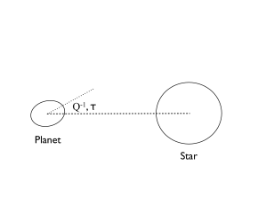
Figure 1.— Schematic of the position of a planetary tidal bulge due to a star. Dissipative processes inside the planet prevent the bulge, marked by the dotted line, from pointing toward the center of the perturber, shown by the dashed line. Instead the bulge points away by an angle that is either inversely proportional to the tidal $Q$ (for the CPL model), or proportional to the time lag $\tau$ (for the CTL model).

2.1. The Constant–Phase–Lag Model

In the “constant-phase-lag” (CPL) model of tidal evolution, the angle between the line connecting the centers of mass and the tidal bulge is constant. Thus, the planet responds to the perturber like a damped, driven harmonic oscillator. The CPL model is commonly used in planetary studies (e.g. Goldreich & Soter, 1966; Greenberg, 2009). Under this assumption, and ignoring the effect of obliquity, the evolution is described by the following equations

$$\frac{\mathrm{d}e}{\mathrm{d}t}\ =\ -\frac{ae}{8GM_{1}M_{2}}\sum\limits_{i=1}^{2}Z^{\prime}_{i}\Bigg{(}2\varepsilon_{0,i}-\frac{49}{2}\varepsilon_{1,i}+\frac{1}{2}\varepsilon_{2,i}+3\varepsilon_{5,i}\Bigg{)}$$ (1)

and

$$\frac{\mathrm{d}a}{\mathrm{d}t}\ =\ \frac{a^{2}}{4GM_{1}M_{2}}\sum\limits_{i=1}^{2}Z^{\prime}_{i}\ {\Bigg{(}}4\varepsilon_{0,i}+e^{2}{\Big{[}}-20\varepsilon_{0,i}+\frac{147}{2}\varepsilon_{1,i}+\frac{1}{2}\varepsilon_{2,i}-3\varepsilon_{5,i}{\Big{]}}{\Bigg{)}}$$

where $e$ is eccentricity, $t$ is time, $a$ is semi-major axis, $G$ is Newton’s gravitational constant, $M_{1}$ and $M_{2}$ are the two masses, and $R_{1}$ and $R_{2}$ are the two radii. The quantity $Z^{\prime}_{i}$ is

$$Z^{\prime}_{i}\equiv 3G^{2}k_{2,i}M_{j}^{2}(M_{i}+M_{j})\frac{R_{i}^{5}}{a^{9}}\ \frac{1}{nQ_{i}}\,$$ (2)

where $k_{2,i}$ are the Love numbers of order 2, $n$ is the mean motion, and $Q_{i}$ are the tidal quality factors. The signs of the phase lags are

$$\begin{array}[]{l}\varepsilon_{0,i}=\Sigma(2\omega_{i}-2n)\\ \varepsilon_{1,i}=\Sigma(2\omega_{i}-3n)\\ \varepsilon_{2,i}=\Sigma(2\omega_{i}-n)\\ \varepsilon_{5,i}=\Sigma(n)\\ \varepsilon_{8,i}=\Sigma(\omega_{i}-2n)\\ \varepsilon_{9,i}=\Sigma(\omega_{i})\ ,\\ \end{array}$$ (3)

where $\omega_{i}$ is the rotational frequency of the $i$th body, which I force to be the equilibrium frequency, $(1+9.5e^{2})n$. $\Sigma(x)$ is the sign of any physical quantity $x$, and thus $\Sigma(x)~{}=~{}+1,-1$, or 0.

2.2. The Constant–Time–Lag Model

The constant-time-lag (CTL) model assumes that the time interval between the passage of the perturber and the tidal bulge is a constant value, $\tau$. This assumption allows the tidal response to be continuous over a wide range of frequencies, unlike the CPL model. But, if the phase lag is a function of the forcing frequency, then the system is no longer analogous to a damped driven harmonic oscillator. Therefore, this model should only be used over a narrow range of frequencies, see Greenberg (2009). Ignoring obliquity, the orbital evolution is described by the following equations:

$$\frac{\mathrm{d}e}{\mathrm{d}t}\ =\ \frac{11ae}{2GM_{1}M_{2}}\sum\limits_{i=1}^{2}Z_{i}\Bigg{(}\frac{f_{4}(e)}{\beta^{10}(e)}\frac{\omega_{i}}{n}-\frac{18}{11}\frac{f_{3}(e)}{\beta^{13}(e)}\Bigg{)}$$ (4)

$$\frac{\mathrm{d}a}{\mathrm{d}t}\ =\ \frac{2a^{2}}{GM_{1}M_{2}}\sum\limits_{i=1}^{2}Z_{i}\Bigg{(}\frac{f_{2}(e)}{\beta^{12}(e)}\frac{\omega_{i}}{n}-\frac{f_{1}(e)}{\beta^{15}(e)}\Bigg{)}$$ (5)

where

$$Z_{i}\equiv 3G^{2}k_{2,i}M_{j}^{2}(M_{i}+M_{j})\frac{R_{i}^{5}}{a^{9}}\ \tau_{i}\ ,$$ (6)

and

$$\begin{array}[]{l}\beta(e)=\sqrt{1-e^{2}},\\ f_{1}(e)=1+\frac{31}{2}e^{2}+\frac{255}{8}e^{4}+\frac{185}{16}e^{6}+\frac{25}{64}e^{8},\\ f_{2}(e)=1+\frac{15}{2}e^{2}+\frac{45}{8}e^{4}\ \ +\frac{5}{16}e^{6},\\ f_{3}(e)=1+\frac{15}{4}e^{2}+\frac{15}{8}e^{4}\ \ +\frac{5}{64}e^{6},\\ f_{4}(e)=1+\frac{3}{2}e^{2}\ \ +\frac{1}{8}e^{4},\\ f_{5}(e)=1+3e^{2}\ \ \ +\frac{3}{8}e^{4}.\end{array}$$ (7)

As in the CPL model, I force the rotational frequency to equal the equilibrium frequency, which is $(1+6e^{2})n$ in the CTL model.

There is no general conversion between $Q_{\mathrm{p}}$ and $\tau_{\mathrm{p}}$. Only if $e~{}=~{}0$ (and the obliquity is 0 or $\pi$), when merely a single tidal lag angle exists, then

$$Q_{\mathrm{p}}~{}\approx~{}1/(2|n-\omega_{\mathrm{p}}|\tau_{\mathrm{p}}),$$ (8)

as long as $n-\omega_{\mathrm{p}}$ remains unchanged. Hence, the canonical values of the dissipation parameters for dry, rocky planets in the Solar System, $Q~{}=~{}100$ (Goldreich & Soter, 1966) and $\tau=64$ s (Lambeck, 1977; Barnes et al., 2013), are not necessarily equivalent. Hence, the results for the tidal evolution will intrinsically differ among the CPL and the CTL model, even though both choices are common for the respective model. While tidal dissipation in super-Earths remains observationally unconstrained, here I will assume that it is similar to the rocky bodies in the Solar System.

2.3. Differential Circularization of Super-Earths and Mini-Neptunes

As described above, most previous research predicts several orders of magnitude difference in $Q$ or $\tau$ between terrestrial and giant planets. As an example in Fig. 2, I simulate the evolution of two hypothetical equal-radius planets with different compositions that formed with identical orbits (5 day period, $e=0.2$) around identical stars. The line shows 10 Gyr of CPL tidal evolution of a $2~{}{\rm\,R_{Earth}}$ planet with a density of 1 g/cm³ (i.e. a gaseous $3.8~{}{\rm\,M_{Earth}}$ mini-Neptune) and a tidal $Q$ of $10^{6}$ (see e.g. Goldreich & Soter, 1966; Jackson et al., 2008b), while the filled circles are the orbit of a $2~{}{\rm\,R_{Earth}}$ planet with a mass of $10~{}{\rm\,M_{Earth}}$ and a tidal $Q$ of 100 (i.e. a super-Earth) every 100 Myr. The super-Earth circularizes in about 1 Gyr; the mini-Neptune barely evolves, even over 10 Gyr. This discrepancy is despite that the equilibrium tidal models predict evolution scales with planetary mass – the large difference between the $Q$s dominates.

Figure 2.— Comparison of the tidal evolution of a gaseous $2~{}{\rm\,R_{Earth}}$ mini-Neptune (solid line; for 10 Gyr) and a rocky $2~{}{\rm\,R_{Earth}}$ super-Earth (open squares; in 100 Myr intervals). Both planets begin with an orbital period of 5 days and and eccentricity of 0.2 and tidally evolve down and to the left. The mini-Neptune experiences little orbital evolution, but the super-Earth circularizes in about 1 Gyr. This discrepancy is due to the 4 orders of magnitude difference in tidal dissipation between gaseous and rocky planets.

3. The Transit Duration Anomaly

In this section I review and revise previous work on the “transit duration anomaly” (TDA), defined here as the ratio of the observed transit duration to the duration if the orbit were circular. This parameter has gone by several names in the literature, such as the “transit duration deviation” (Kane et al., 2012), and the “photoeccentric effect” (Dawson & Johnson, 2012). Here I use the name proposed by Plavchan et al. (2012), as in celestial mechanics the term “anomaly” refers to a parameter’s value relative to pericenter, e.g. the “true anomaly” is the difference between a planet’s true longitude and its longitude of pericenter. The analogy is not perfect, as the TDA is not measured relative to the duration at pericenter, but rather to the duration due to a circular orbit. Nonetheless, “anomaly” captures the fact that the duration is set by the longitude relative to pericenter, the true anomaly $\theta$, as shown below.

In this section, I first review how the TDA can be used to determine the minimum eccentricity of an orbit. Then I review the biases implicit in TDA measurements and update previous results.

3.1. Determination of the Minimum Eccentricity

Transit data coupled with knowledge of semi-major axis enable the imposition of a lower bound on the eccentricity $e_{min}$ (Jason W. Barnes 2007; Ford et al. 2008). The determination of $e_{min}$ requires knowledge of both the physical size of the orbit, as well as a precise determination of the orbital period $P$, planetary and stellar radii ($R_{p}$ and $R_{*}$), and the impact parameter $b$, see Fig. 3. If the transit is well-sampled, then these parameters can be obtained (Mandel & Agol, 2002).

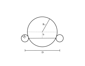
Figure 3.— Schematic of a planetary transit. The planet has a radius $R_{p}$, and the star $R_{*}$. The planet crosses the stellar disk a projected distance $b$ from disk center. The distance the planet travels during transit is $D$, the distance between the center of the planet at first and fourth contacts.

The transit duration is the time required for a planet to traverse the disk of its parent star, and to first order is:

$$T=\frac{D}{v_{sky}}=\frac{2(\sqrt{(R_{*}+R_{p})^{2}-b^{2}}}{v_{sky}},$$ (9)

where $v_{sky}$ is the azimuthal velocity, i.e. the instantaneous velocity of the planet in the plane of the sky. Although several different definitions of the duration are possible (Kipping, 2010), I choose this definition to match the Kepler public data. On a circular orbit, the azimuthal velocity is constant and equal to the orbital velocity. Therefore the duration for a circular orbit is

$$T_{c}=\frac{\sqrt{(R_{*}+R_{p})^{2}-b^{2}}}{\pi a}P,$$ (10)

where $P$ is the orbital period. For an eccentric orbit the orbital velocity is a function of longitude (Kepler’s 2nd Law), and is given by

$$v=v_{c}\sqrt{\frac{1+2e\cos\theta+e^{2}}{1-e^{2}}},$$ (11)

where $e$ is the eccentricity and $v_{c}$ is the circular velocity. Finally, from classical mechanics, the azimuthal velocity is

$$v_{sky}=v_{c}\frac{1+e\cos\theta}{\sqrt{1-e^{2}}}.$$ (12)

From transit data alone, the value of $\theta$ is unknown, and hence so is $e$.

However, one can exploit the difference between $T$ and $T_{c}$ to obtain a minimum value of the eccentricity, $e_{min}$ (Barnes, 2007). The situation is somewhat complicated because $T$ can be larger or smaller than $T_{c}$ depending on $\theta$. If the planet is close to apoapse, $T>T_{c}$, while near periapse $T<T_{c}$. To derive $e_{min}$, one must assume that $\theta=0$ or $\pi$. While the velocity could be larger at some other position in the orbit, the maximum deviation from the circular velocity is at least as large as the measured velocity, and hence $e$ must be at least a certain value. If I define the TDA as

$$\Delta\equiv T/T_{c}=v_{c}/v_{sky}=\frac{\sqrt{1-e^{2}}}{1+e\cos\theta},$$ (13)

then

$$e_{min}=\left|\frac{\Delta^{2}-1}{\Delta^{2}+1}\right|$$ (14)

is the minimum eccentricity permitted by transit data.

Several studies invoked the orbital velocity instead of the sky velocity (e.g.  Tingley & Sackett, 2005; Burke, 2008; Kipping, 2010). However, J. W. Barnes (2007) correctly noted that $T$ is actually a function of the azimuthal velocity, which equals the orbital velocity at pericenter and apocenter. For many other studies, the assumed form of the velocity is unclear. As transits are a photometric phenomenon, unaffected by the component of the velocity along the line of sight, the projection of the orbital velocity into the sky plane, $v_{sky}$, is the appropriate choice. This implies that previous studies are only approximately correct. As I show in the next section, using $v_{c}$ will only amount to a small error.

The TDA has been used in several studies to constrain the eccentricity distribution, often with the assumption that the impact parameter is unknown, as proposed by Ford et al. (2008). In that case, one can only use those systems in which $T>T_{c}$ for a central transit ($b=0$) to estimate $e_{min}$. Moorhead et al. (2011) analyzed the first 3 quarters of Kepler data and found that the KOIs appeared to be consistent with a mean eccentricity near 0.2. They also found that eccentricities appear to be large regardless of orbital period, and that small planets tend to have larger eccentricities. More recent work has failed to determine if the Kepler eccentricity distribution is consistent with the radial velocity planets (Plavchan et al., 2012; Kane et al., 2012). These studies were limited by the number of known candidates, as well as the relatively poor characterization of the transits themselves. Note that Kane et al. (2012) used the difference between $T$ and $T_{c}$, rather than the quotient, to model eccentricity. Dawson & Johnson (2012) demonstrated that in some cases careful statistical analyses of transit data can provide constraints on the actual eccentricity, especially if $\Delta$ deviates significantly from unity.

3.2. Observational Biases in the Transit Duration Anomaly

To further elucidate the TDA, as well as to revisit previous results that may have invoked an inappropriate definition, in this section I review the geometry and biases associated with it. In Fig. 4 I show the orbital and and azimuthal velocities as a function of true anomaly for three different eccentricities. The differences between the panels are subtle at low $e$, but can be significant for large $e$.

Figure 4.— Velocity relative to the circular velocity as a function of true anomaly for three different eccentricities. The dotted line shows the circular velocity. Dashed lines show the values of true anomaly at which the velocity equals the circular velocity. Left: Orbital velocity. Right: Velocity in the plane of the sky.

The vertical lines in Fig. 4 show the values of $\theta$ at which the velocity is equal to the circular velocity. For the orbital velocity, the longitude where $v=v_{c}$ is given by

$$\theta_{c}^{orb}=\pm\cos^{-1}(-e)$$ (15)

and for the azimuthal velocity, it lies at

$$\theta_{c}^{sky}=\pm\cos^{-1}\Big{(}\frac{\sqrt{1-e^{2}}-1}{e}\Big{)}.$$ (16)

In Fig. 5, I show schematics for 4 orbits. In all cases an observer at $x=+\infty$ views the transit such that either $v=v_{c}$ (left) or $v_{sky}=v_{c}$ (right).

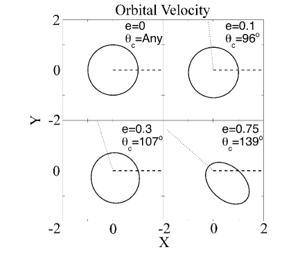
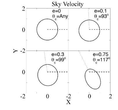
Figure 5.— Locations on an orbit where a velocity is equal to the circular velocity. In all cases, the orbit’s semi-major axis is 1, and the observer is assumed to be located at $x=+\infty$, as shown by the dashed line. The longitude of periastron is shown by the dotted line. In each panel the eccentricity is listed, as is one of the values of the true anomaly at which the velocity is circular. In all cases, the orbit is rotated so that that longitude, $\theta_{c}$, lies on the $+x$-axis. Left: The total velocity of the planet is equal to the circular velocity when it crosses the $+x$ axis. In these cases, the observer will see transit durations longer than that from an identical planet on a circular orbit. Right: The azimuthal velocity is equal to the circular velocity when it crosses the $+x$ axis. In these cases, an observer will see a transit duration equal to that of an identical planet, but on a circular orbit, i.e. $e_{min}=0$.

As I am only interested in the azimuthal velocity, for the remainder of this paper I will assume that $\theta_{c}=\theta_{c}^{sky}$ and drop the superscript. For an eccentric orbit, the planet travels faster than the circular velocity for $\theta_{c}/\pi>0.5$ of the orbit. There is therefore an observational bias, which I will call the “velocity bias,” to observe $\Delta<1$ (Tingley & Sackett, 2005; Burke, 2008; Plavchan et al., 2012). The probability that $T<T_{c}$ due to this effect is just

$$p_{vel}(T<T_{c})=\frac{\theta_{c}}{\pi}$$ (17)

and is shown by the dashed curve in Fig. 6.

The bias toward small $\Delta$ is magnified by the geometrical bias toward transits occurring at smaller star-planet separations. As shown in J. W. Barnes (2007; see also Borucki & Summers 1984), the overall transit probability is

$$p_{transit}=\frac{1}{4\pi}\frac{2R_{*}}{a(1-e^{2})}\int_{0}^{2\pi}(1+e\cos\theta)d\theta=\frac{R_{*}}{a(1-e^{2})}$$ (18)

and the probability to observe the transit when $T<T_{c}$ is

$$p_{short}=\frac{1}{4\pi}\frac{2R_{*}}{a(1-e^{2})}\int_{-\theta_{c}}^{\theta_{c}}(1+e\cos\theta)d\theta=\frac{R_{*}(\theta_{c}+e\sin\theta_{c})}{a\pi(1-e^{2})},$$ (19)

and thus the bias toward observing a transit duration shorter than the circular duration is the ratio of these two equations,

$$p_{duration}=\frac{\theta_{c}+e\sin(\theta_{c})}{\pi},$$ (20)

which I will call the “duration bias.” This effect is shown by the solid curve in Fig. 6, and is the actual likelihood to observe a transit with $T<T_{c}$. As $e\rightarrow 1$, it becomes extremely unlikely to observe a long transit. This effect can make studies that rely on transit durations longer than that predicted for a central transit ($b=0$) unlikely to find high eccentricity objects (e.g. Moorhead et al., 2011; Plavchan et al., 2012).

Figure 6.— Probability of detecting a transit duration shorter than that of a planet on a circular orbit. The dashed curve is the “velocity bias” that arises because more longitudes have $v_{sky}>v_{c}$. The solid curve is the “duration bias” that also takes into account the increased transit probability when the star-planet separation is small. The solid curve is the actual bias, which is not a straight line.

In practice, this bias is not dramatic as most planets are not on very eccentric orbits. Burke (2008) used analytic fits to the then-current eccentricity distribution as determined from radial velocity planets, excluding those with orbital periods less than 10 days that may be tidally circularized, to find that the mean value of $\Delta$ should be 0.88. Recall that Burke (2008) used $v$ instead of $v_{sky}$ in his definition of $\Delta$, thus his mean should be slightly lower than the actual mean as $v~{}\geq~{}v_{sky}$.

To update the expectations of Burke (2008), I recompute the expected distribution of $\Delta$ from radial velocity planets. In the left panel of Fig. 7, I show the current distribution of $e$ with the thick gray line. I exclude those planets with $a>0.1$ AU leaving 362 planets. To evaluate the expected distribution of $\Delta$, I created $10^{7}$ synthetic systems consisting of a star with a radius between 0.7 and 1.4 R_☉, and a planet whose radius I ignored. The orbit had $a=0.05$ AU, an eccentricity distribution given by the dashed histogram in the left panel of Fig. 7, and an isotropic distribution of orbits. I then calculated $\Delta$ for all transiting geometries with durations larger than 1 hour and show the resulting $\Delta$ distribution in the right panel of Fig. 7. As noted, 66% of cases have $\Delta<1$, with a mean value of 0.90. If I instead use the circular velocity to calculate $\Delta$, I find 68% have $\Delta<1$, with a mean of 0.88, reproducing the Burke (2008) result. The difference between using $v_{c}$ and $v_{sky}$ to calculate the TDA is modest for the known radial-velocity-detected planets.

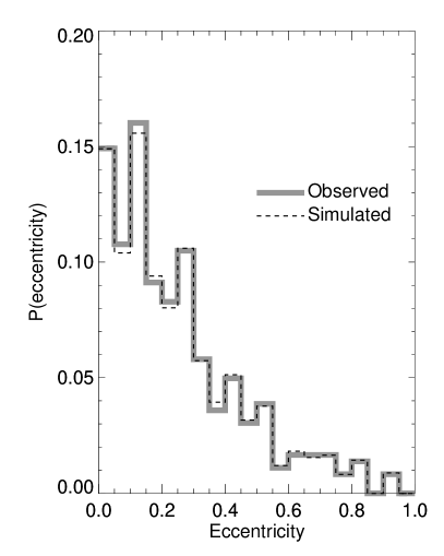
Figure 7.— Left: Eccentricity distribution of exoplanets. The solid gray line is the observed distribution (with bin size 0.05) of 362 radial velocity exoplanets with $a>0.1$ AU from exoplanets.org as of 4 June 2013. The dashed line is the distribution used in this study. Right: The transit duration anomaly expected from the simulated data set assuming a random viewing geometry and that the transit duration is set by the azimuthal velocity, Eq. (12).

4. Methodology

In order to determine if the difference in $Q$ values can permit the identification of $R_{crit}$, I perform Monte Carlo simulations of both the CPL and CTL models. I then compare the results to publicly-available Kepler data to search for the predicted signal.

For my synthetic data, I created 25,000 star-planet configurations with initial semi-major axes uniformly in the range [0.01,0.15] AU, planetary radii in the range [0.5,10] ${\rm\,R_{Earth}}$, stellar masses in the range [0.7,1.4] ${\rm\,M_{Sun}}$, a radius in solar radii equal to its mass in solar masses, and ages in the range [2,8] Gyr. If the planetary radius is less than $2~{}{\rm\,R_{Earth}}$, then the mass is $(R/{\rm\,R_{Earth}})^{3.68}{\rm\,M_{Earth}}$ (Sotin et al., 2007), if larger, then I assume the density is 1 g/cm³, similar to the planets in the Kepler-11 system (Lissauer et al., 2013). The initial eccentricity is drawn from the currently observed distribution of distant planets ($a>0.1$ AU), see Fig. 7. For CPL runs I randomly choose tidal parameters in the ranges $30\leq Q_{r}\leq 300$, $10^{6}\leq Q_{g}\leq 10^{7}$, and $10^{6}\leq Q_{*}\leq 10^{7}$. For CTL runs I used $30\leq\tau_{r}\leq 300$ s, $0.003\leq\tau_{g}\leq 0.03$ s, and $0.001\leq\tau_{*}\leq 0.01$ s. I then integrated the system forward for the randomly chosen age and assumed I observed the system in that final configuration. In order to calculate $e_{min}$, I choose a random value for $\theta$ that represents the direction of the observer, and an inclination $i$ chosen uniformly in $\cos i$, with $i$ measured from the plane of the sky. I then calculate the separation between the star and planet using

$$r=\frac{a(1-e^{2})}{1+e\cos\theta}$$ (21)

and determine the impact parameter, $b=r\tan(\pi/2-i)$. If $b<R_{*}$, then the planet transits, and I calculate the transit duration. As pointed out in Burke (2008), short transit durations can be missed, and I therefore throw out transit durations that are less than 1 hour, which is the approximate minimum duration detectable by Kepler. The vast majority of the rejected transits are too short due to a large impact parameter, however a few are due to large eccentricity and alignment of the longitude of pericenter with the line of sight. Thus, my estimates of the minimum eccentricity distribution are slightly biased toward lower values. From the remaining transits, I calculate the TDA and $e_{min}$ using Eqs. (12–14).

I also compute $e_{min}$ for Kepler candidates that have all the requisite parameters presented in Kepler Planet Candidate Data Explorer (see also Batalha et al., 2013). These data do not contain error bars and assuredly contain some false positive, but the data set is uniform and sufficient for this proof of concept. I limit my sample to those with orbital periods less than 15 days, but will refer to this subsample as the “Kepler sample” in the upcoming sections.

5. Results

5.1. Tides and the Minimum Eccentricity

I begin by considering an intermediate step: In Fig. 8, I show the average final eccentricity of my simulated planets as a function of planetary radius, $R_{p}$, and orbital period, $P$. The paucity of eccentric orbits at low $R_{p}$ and $P$ shows the more effective circularization of rocky bodies. Furthermore, I can see the features that correspond directly to three parameters that are currently very poorly constrained: $R_{crit}$ via the rapid rise in $<e>$ at the imposed value of $2~{}{\rm\,R_{Earth}}$; $Q_{g}$ ($\tau_{g}$) via the rapid rise in $<e>$ at 1 day above $2~{}{\rm\,R_{Earth}}$; and $Q_{r}$ ($\tau_{r}$) via the rise over 2–10 days and below $2~{}{\rm\,R_{Earth}}$. Thus, despite the order of magnitude uncertainty I gave to each physical parameter, the large discrepancy between $Q_{r}$ ($\tau_{r}$) and $Q_{g}$ ($\tau_{g}$) does result in an important difference in the expected orbits of close-in planets of FGK stars. For the CTL model, 1,955 planets merged with the star during the integrations; 1,118 for CPL (see Jackson et al., 2009; Levrard et al., 2009).

Figure 8.— Average final eccentricity of a suite of $\sim 23,000$ systems of one star and one planet that experienced tidal evolution for 2–8 Gyr. Planets larger than $2~{}{\rm\,R_{Earth}}$ are gaseous, and those smaller are rocky. The binsizes are $0.5~{}{\rm\,R_{Earth}}$  in radius and 0.5 d in period. Gaseous planets retain a residual eccentricity if $P>1.5$ d, while rocky planets require $P>3$ d. The transition occurs at $2~{}{\rm\,R_{Earth}}$, which in this case is $R_{crit}$. Left: Orbits evolve according to the constant-time-lag model. Right: Orbits evolve according to the constant-phase-lag model.

Next I calculate the average minimum eccentricity $<e_{min}>$ for transiting geometries of simulated rocky and gaseous planets in 0.5 day orbital period intervals and plot $<e_{min}>$ as a function of orbital period for different radii as solid lines in Fig. 9. For the CTL model, I obtained 2,127 observable transits, and for CPL 2,151, about twice as many planets as in the same period range as the Kepler sample. Note that my synthetic data do not share several properties of the Kepler data, such as the planetary radius and period distributions. For both the CTL (left) and CPL (right) models, the trends are the same. For $R<R_{crit}$, $<e_{min}>\sim 0$ up to about a 4–5 day period. However, for larger radii, circular orbits are only guaranteed for periods less than about 1.5–2 days. The rocky and gaseous distributions become about equal at $P=13$ days, albeit with considerable scatter. At large orbital periods, the simulated data become sparser as the transit probability is dropping (producing the apparent oscillations in $<e_{min}>$), and those that do transit are more likely to be near pericenter of an eccentric orbit, causing the secular growth in $<e_{min}>$ with period. Note that similar variations are present in the Kepler sample.

Figure 9.— Average minimum eccentricities for transiting exoplanets as a function of period and radius. The solid curve and filled squares represent planets with radii below the selected critical radius of $2~{}{\rm\,R_{Earth}}$, while the dashed curve and open circles are larger planets. The lines are for the simulated data set incorporating the duration bias, symbols for KOIs. The latter have values of $<e_{min}>$ of 0.2–0.5 regardless of period, whereas model gaseous planets have non–zero eccentricities if the period is larger than 1.5 days, and rocky planets at larger than 4. If tidal dissipation is a function of exoplanet radius, it should be detectable. Left: Results for the CTL model. Right: Results for the CPL model.

Figure 9 also contains the values of $e_{min}$ provided by the Kepler team as squares. Solid squares correspond to $R_{p}<R_{crit}$, open to $R_{p}>R_{crit}$. Nearly all the observed data are above the predictions, in agreement with the results of Moorhead et al. (2011). Therefore, it does not appear that there is any signal of tidal evolution in the Kepler data, regardless of orbital period! This result is in stark contrast to radial velocity data that show clear signs of circularization at small $P$ (e.g.  Butler et al., 2006). Moreover, the average eccentricity in the Butler et al. catalog is $\sim 0.25$, which is lower than the vast majority of minimum eccentricities derived from Kepler transits in this study. As the radial velocity data are older and have been reproduced by multiple teams, the Kepler data are more likely to be incorrect. In the next section I describe several plausible explanations for the discrepancy.

5.2. A Closer Look at the Kepler Sample

The lack of evidence of tidal evolution in the KOIs suggests there is an issue with the interpretation of the light curves. In this section I examine several features of the Kepler sample and conclude that the data suffer from a systematic bias. As described in Batalha et al. (2013), transits are fit to the geometric, limb-darkened transit model of Mandel & Agol (2002). This model can determine planetary radius and impact parameter, as well as other parameters that are not relevant to the current study. The publicly-available data are long cadence, and hence the transits are not well-sampled. This sparse sampling is most likely to affect the impact parameter, as the shape of the transit is crucial to its estimation. Below I show that the impact parameters do indeed appear to be suspicious.

A partial list of the Kepler data used in this study is shown in Table 1, with the full table available in the supplementary material. In Fig. 10 I plot $\Delta$ as a function of orbital period in the left panel. Although no trends are present, it does appear that most values of $\Delta$ are greater than 1. In the right panel I bin the $\Delta$ values to confirm this impression. This distribution cannot be explained by orbital mechanics and isotropic orbits which predict that $\Delta$ distributions can only be biased toward $\Delta<1$. Instead I find 78% of KOIs have $\Delta>1$, with a mean value of 1.38.

Figure 10.— The transit duration anomalies of the KOIs in the sample (which are short-period). Left: TDA as a function of orbital period. Right: The histogram of TDA values shows that most values are larger than 1.

To search for the source of this discrepancy, I considered relationships among the parameters that permit the calculation of $e_{min}$. The durations increase monotonically with the orbital period, albeit with significant scatter, as expected (Kane et al., 2012). Several studies have pointed out systematic errors in the stellar characterization (Dressing & Charbonneau, 2013; Everett et al., 2013). In particular, Everett et al. (2013) studied 220 Kepler host stars and found the vast majority have larger radii than reported by the Kepler team, and that one-quarter are 35% larger than suggested by the Kepler team. Since $\Delta~{}\propto~{}R_{*}^{-1}$, such a revision could significantly lower $\Delta$ and potentially resolve the discrepancy. Since they “only” examined 220 host stars, some of which are not known to host a close-in planet, I do not include their results here, so that my analysis is kept to a uniform sample.

Table 1. Properties of Short Period KOIs

KOI	$a$ (AU)	$P$ (d)	$T$ (hr)	$R_{p}$ (REarth)	$R_{*}$ (RSun)	$b$	$T_{c}$ (hr)	$\Delta$	$e_{min}$
1.01	0.036	2.471	1.732	14.42	1.06	0.822	1.984	0.873	0.135
2.01	0.039	2.205	3.877	22.29	2.71	0.128	5.810	0.667	0.384
3.01	0.052	4.888	2.368	4.67	0.74	0.029	2.612	0.907	0.098
4.01	0.056	3.849	2.928	11.79	2.60	0.946	2.764	1.059	0.058
5.01	0.058	4.780	2.012	5.65	1.42	0.951	1.716	1.172	0.158
5.02	0.075	7.052	3.688	0.66	1.42	0.750	3.169	1.164	0.151
7.01	0.044	3.214	4.111	3.72	1.27	0.714	2.431	1.691	0.482
10.01	0.047	3.522	3.198	15.88	1.56	0.640	3.682	0.869	0.140
17.01	0.045	3.235	3.602	11.06	1.08	0.029	3.015	1.195	0.176
18.01	0.052	3.548	4.081	17.37	2.02	0.006	5.282	0.773	0.252
20.01	0.056	4.438	4.671	17.58	1.38	0.018	4.338	1.077	0.074
…

Perhaps the biggest inconsistency in the Kepler data lies in the impact parameter, see Fig. 11. The distribution predicted by the radial velocity exoplanets beyond the reach of tides is shown with the dashed histogram and is taken from the same sample that produced the right panel of Fig. 7. It is approximately flat, with the slight rise toward small values due to isotropically distributed orbits favoring edge-on geometries. Instead, the Kepler sample, shown by the solid line, rises sharply to large values of $b$. This distribution hints that a systematic error may be present in the Kepler analysis, which manifests itself in my analysis into large values of $\Delta$ and $e_{min}$. I conclude that the currently available Kepler data produce unreliable values of $b$ and hence $e_{min}$.

Figure 11.— Distribution of impact parameters. The expected distribution of the radial velocity exoplanets with no tidal circularization is shown by the dashed line. The short-period KOIs tend to have large impact parameters.

6. Discussion

My simulated data show that $R_{crit}$ is identifiable in transit data due to the difference in the tidal $Q$s of gaseous and rocky bodies, at least for my idealized model of exoplanetary properties. My analysis is somewhat circular as I split the data in Fig. 9 on the selected value of $R_{crit}$. In reality, its value is unknown and must be searched for. However, given the large and approximately equal values of $<e_{min}>$ in the Kepler data, I did not perform that search. More accurate data are needed, and may be available as KOI parameters are refined. Resolution of transit ingress and egress may be possible with short cadence data (which are unpublished but assuredly a small fraction of the total number of KOIs), or by folding the hundreds of transits together (e.g., Jackson et al., 2013), potentially rectifying the discordance between the Kepler and radial velocity data.

In order to accurately determine the minimum eccentricities, one needs reliable information for both $R_{*}$ and $b$, but it is not yet available. Although subsets of more reliable data are available for the former (e.g.  Everett et al., 2013), the transit fits are still plagued by inaccurate calculations of the impact parameter. Determination of the impact parameters in short cadence data or by folding would require a new and comprehensive analysis of those light-curves and is beyond the scope of this study. After those data have been properly analyzed, the technique described in this study should be re-applied in order to determine $R_{crit}$, $Q_{g}$, and $Q_{r}$.

Aside from systematic errors in the analysis of the light curves, physical effects can also impact the value of $<e_{min}>$. First, I note that additional companions can pump eccentricity through mutual gravitational interactions, even if tidal damping is ongoing (Mardling & Lin, 2002; Bolmont et al., 2013). Therefore one must be cautious when interpreting Fig. 9, as additional companions, both seen and unseen, can maintain non–zero eccentricities. However, Bolmont et al. (2013) showed that planet–planet interactions cannot maintain the eccentricity of the hot super-Earth 55 Cnc e above 0.1. That system is particularly relevant as there are many close–in planets orbiting a typical G dwarf. Therefore, I conclude that eccentricity pumping can be significant, but cannot explain the discrepancy between the observed and simulated systems shown in Fig. 9. This analysis should be revisited when all the Kepler data become available and all issues with host star characterization have been resolved.

Another possibility is that stellar winds and activity can strip an atmosphere, reducing the mass and radius, and potentially changing the planet from a mini–Neptune to a super–Earth (Jackson et al., 2010; Valencia et al., 2010; Leitzinger et al., 2011; Poppenhaeger et al., 2012). Recently, Owen & Wu (2013) argued that the Kepler sample is consistent with hydrodynamic mass loss, and that some low–mass planets could have formed with substantially more mass. Mass loss should increase the time to circularize the orbit, assuming the radius doesn’t become very large, which is unlikely after about 100 Myr (Lopez et al., 2012). Therefore, mass loss could stall circularization for mini–Neptunes, but not for super–Earths. Although few radial velocity measurements exist for planets with radii less than $\sim 1.5~{}{\rm\,R_{Earth}}$, they have densities consistent with silicate compositions (Batalha et al., 2011). Thus, mass loss seems unlikely to explain the differences seen for the smallest candidates in the Kepler field.

Radial inflation by irradiation (e.g.  Lopez et al., 2012) or tidal heating (Bodenheimer et al., 2001; Jackson et al., 2008c; Ibgui & Burrows, 2009) also work to decrease $e$ since the evolution scales as $R_{p}^{5}$. Hence, bloated planets should be found on circular orbits, but no such trend is observed in the Kepler candidates.

In this study I used two qualitatively different equilibrium tidal models and standard assumptions for dissipation. However different tidal models have been proposed (e.g. Ogilvie & Lin, 2004; Henning et al., 2009; Socrates et al., 2012; Makarov & Efroimsky, 2013) and could be applied to this problem. The trend I predict here holds unless the dissipation rates in gas giants and rocky planets are within 1–2 orders of magnitude of each other, rather 4–6. Recently, Storch & Lai (2013) have proposed just such a model in which all tidal dissipation in gas giants occurs in a rocky core. Should all planets show the same trend in $e_{min}$, then that would be evidence in support of their model. Hence, even if the expectations laid out above prove to be incorrect, some tidal models could be rejected by the methodology used in this study.

I have focused on transiting planets, but an analogous study could be applied to radial velocity data. Those data may be more amenable to such a study as orbital eccentricity is a direct observable. The problem lies in the low reflex velocities induced by the small planets as well as the ambiguity in mass due to the mass-inclination degeneracy. Nonetheless, with enough objects and an accounting for the expected isotropy of orbits, it may be possible to determine tidal dissipation as a function of mass in radial velocity data.

The Kepler spacecraft was designed to discover a potentially habitable planet orbiting a solar-like star. Such a planet ($m_{p}~{}\hbox to0.0pt{$<$\hss}{\lower 4.30554pt\hbox{$\sim$}}10~{}{\rm\,M_{Earth}}$; $r_{p}~{}\hbox to0.0pt{$<$\hss}{\lower 4.30554pt\hbox{$\sim$}}2~{}{\rm\,R_{Earth}}$; $P\approx 1$ year) would have an undetectable radial velocity signature, preventing a direct mass measurement. Thus, confirmation of that planet’s rocky nature is daunting. However, Kepler data may also hold the key to a convincing solution to the problem, as shown in this study. The distribution of TDAs in conjunction with tidal theory suggests the value of $R_{crit}$ may be calculated from the close-in planets. Although these planets are not habitable, they may provide crucial information to assess the habitability of Earth-like planets that transit Sun-like stars.

7. Conclusions

I have shown that the expected difference in tidal dissipation between gaseous and terrestrial exoplanets should lead to tidal circularization at different orbital distances. I have also shown how transit data, namely the transit duration anomaly, can be used to determine the critical radius between gaseous and terrestrial planets. Moreover, an analysis of $e_{min}$ can also constrain the tidal dissipation in exoplanets, an understanding of which is sorely needed. Using standard values for tidal parameters and the critical radius, I find that a large ensemble of transit data should identify the critical radius between rocky and gaseous exoplanets. My analysis of available Kepler data reveals that the theoretical expectations are not met. However, this discrepancy cannot be used to refute the hypothesis because the values of $<e_{min}>$ are inconsistent with radial velocity detected exoplanets, particularly where tidal damping has been observed.

I have also reviewed the derivation of the TDA, as well as the known biases toward small values. Previous studies have advocated different choices for the velocity of the transiting planet as a function of true anomaly. The transit duration is actually determined by the azimuthal velocity, which is the velocity in the sky plane (Eq. [12]). While it is not clear in all previous studies which velocity was used, those that used the orbital velocity will obtain slightly smaller expected values of $\Delta$. I find that the current distribution of exoplanet eccentricities predicts that 66% of transit durations should be less than $T_{c}$, with a mean and mode of 0.9. In contrast, 78% of short-period KOIs have durations greater than $T_{c}$ with a mean of 1.38. This distribution is inconsistent with celestial mechanics and the expectation isotropic orbits, regardless of tidal damping.

As the Kepler data are refined, or as new data, e.g. from the TESS mission arrive, this hypothesis should be revisited. The value of $R_{crit}$ is crucial for the interpretation of the habitability of transiting Earth-sized planets orbiting Sun-sized stars. Moreover, planets in the habitable zones of M dwarfs are susceptible to tidal effects (Dole, 1964; Kasting et al., 1993; Jackson et al., 2008a; Heller et al., 2011; Barnes et al., 2013), so a determination of $Q$ for terrestrial exoplanets is also crucial to assessing habitability of planets such as those orbiting Gl 581 (Udry et al., 2007; Mayor et al., 2009; Vogt et al., 2010) and Gl 667C (Anglada-Escudé et al., 2012; Bonfils et al., 2013; Anglada-Escudé et al., 2013). As missions like Kepler and TESS have been designed to find potentially habitable worlds, the determination of $R_{crit}$ through their data alone would be an important step forward in determining the occurrence rate of terrestrial planets in the HZ.

Acknowledgments
I thank Andrew Becker, Eric Agol, Leslie Hebb, Jason Barnes, Brian Jackson and René Heller for helpful discussions. This work was supported by NSF grant AST-110882 and the NAI’s Virtual Planetary Laboratory lead team. I also thank an anonymous referee and Nader Haghighipour for reviews that greatly improved the clarity and accuracy of this manuscript.

References

- Agol et al. (2005) Agol, E., Steffen, J., Sari, R., & Clarkson, W. 2005, MNRAS, 359, 567
- Anglada-Escudé et al. (2012) Anglada-Escudé, G., Arriagada, P., Vogt, S. S., et al. 2012, ApJ, 751, L16
- Anglada-Escudé et al. (2013) Anglada-Escudé, G., Tuomi, M., Gerlach, E., et al. 2013, A&A, 556, A126
- Barnes (2007) Barnes, J. W. 2007, PASP, 119, 986
- Barnes et al. (2013) Barnes, R., Mullins, K., Goldblatt, C., et al. 2013, Astrobiology, 13, 225
- Batalha et al. (2011) Batalha, N. M., Borucki, W. J., Bryson, S. T., et al. 2011, ApJ, 729, 27
- Batalha et al. (2013) Batalha, N. M., Rowe, J. F., Bryson, S. T., et al. 2013, ApJS, 204, 24
- Bodenheimer et al. (2001) Bodenheimer, P., Lin, D. N. C., & Mardling, R. A. 2001, ApJ, 548, 466
- Bolmont et al. (2013) Bolmont, E., Selsis, F., Raymond, S. N., et al. 2013, ArXiv e-prints, arXiv:1304.0459
- Bonfils et al. (2013) Bonfils, X., Delfosse, X., Udry, S., et al. 2013, A&A, 549, A109
- Boyajian et al. (2012) Boyajian, T. S., von Braun, K., van Belle, G., et al. 2012, ApJ, 757, 112
- Burke (2008) Burke, C. J. 2008, ApJ, 679, 1566
- Butler et al. (2006) Butler, R. P., Wright, J. T., Marcy, G. W., et al. 2006, Astrophys. J., 646, 505
- Darwin (1880) Darwin, G. H. 1880, Royal Society of London Philosophical Transactions Series I, 171, 713
- Dawson & Johnson (2012) Dawson, R. I., & Johnson, J. A. 2012, ApJ, 756, 122
- Dole (1964) Dole, S. H. 1964, Habitable planets for man
- Dressing & Charbonneau (2013) Dressing, C. D., & Charbonneau, D. 2013, ApJ, 767, 95
- Efroimsky & Williams (2009) Efroimsky, M., & Williams, J. G. 2009, Celestial Mechanics and Dynamical Astronomy, 104, 257
- Everett et al. (2013) Everett, M. E., Howell, S. B., Silva, D. R., & Szkody, P. 2013, ApJ, 771, 107
- Ferraz-Mello et al. (2008) Ferraz-Mello, S., Rodríguez, A., & Hussmann, H. 2008, Celestial Mechanics and Dynamical Astronomy, 101, 171
- Ferraz-Mello et al. (2011) Ferraz-Mello, S., Tadeu Dos Santos, M., Beaugé, C., Michtchenko, T. A., & Rodríguez, A. 2011, A&A, 531, A161
- Ford et al. (2008) Ford, E. B., Quinn, S. N., & Veras, D. 2008, ApJ, 678, 1407
- Goldreich & Soter (1966) Goldreich, P., & Soter, S. 1966, Icarus, 5, 375
- Greenberg (2009) Greenberg, R. 2009, Astrophys. J., 698, L42
- Guillot (2005) Guillot, T. 2005, Annual Review of Earth and Planetary Sciences, 33, 493
- Heller et al. (2011) Heller, R., Leconte, J., & Barnes, R. 2011, Astro. & Astrophys., 528, A27+
- Henning et al. (2009) Henning, W. G., O’Connell, R. J., & Sasselov, D. D. 2009, Astrophys. J., 707, 1000
- Holman & Murray (2005) Holman, M. J., & Murray, N. W. 2005, Science, 307, 1288
- Holman et al. (2010) Holman, M. J., Fabrycky, D. C., Ragozzine, D., et al. 2010, Science, 330, 51
- Hubickyj et al. (2005) Hubickyj, O., Bodenheimer, P., & Lissauer, J. J. 2005, Icarus, 179, 415
- Hut (1981) Hut, P. 1981, Astro. & Astrophys., 99, 126
- Ibgui & Burrows (2009) Ibgui, L., & Burrows, A. 2009, Astrophys. J., 700, 1921
- Ikoma et al. (2001) Ikoma, M., Emori, H., & Nakazawa, K. 2001, ApJ, 553, 999
- Jackson et al. (2008a) Jackson, B., Barnes, R., & Greenberg, R. 2008a, MNRAS, 391, 237
- Jackson et al. (2009) —. 2009, Astrophys. J., 698, 1357
- Jackson et al. (2008b) Jackson, B., Greenberg, R., & Barnes, R. 2008b, Astrophys. J., 678, 1396
- Jackson et al. (2008c) —. 2008c, Astrophys. J., 681, 1631
- Jackson et al. (2010) Jackson, B., Miller, N., Barnes, R., et al. 2010, Mon. Not. R. Astron. Soc., 407, 910
- Jackson et al. (2013) Jackson, B., Stark, C. C., Adams, E. R., Chambers, J., & Deming, D. 2013, ArXiv e-prints, arXiv:1308.1379
- Kane et al. (2012) Kane, S. R., Ciardi, D. R., Gelino, D. M., & von Braun, K. 2012, MNRAS, 425, 757
- Kasting et al. (1993) Kasting, J. F., Whitmire, D. P., & Reynolds, R. T. 1993, Icarus, 101, 108
- Kipping (2010) Kipping, D. M. 2010, MNRAS, 407, 301
- Kopparapu et al. (2013) Kopparapu, R. K., Ramirez, R., Kasting, J. F., et al. 2013, ApJ, 765, 131
- Lainey et al. (2012) Lainey, V., Karatekin, Ö., Desmars, J., et al. 2012, ApJ, 752, 14
- Lambeck (1977) Lambeck, K. 1977, Royal Society of London Philosophical Transactions Series A, 287, 545
- Leconte et al. (2010) Leconte, J., Chabrier, G., Baraffe, I., & Levrard, B. 2010, Astro. & Astrophys., 516, A64+
- Léger et al. (2009) Léger, A., Rouan, D., Schneider, J., et al. 2009, Astro. & Astrophys., 506, 287
- Leitzinger et al. (2011) Leitzinger, M., Odert, P., Kulikov, Y. N., et al. 2011, Planet. Space Sci., 59, 1472
- Levrard et al. (2009) Levrard, B., Winisdoerffer, C., & Chabrier, G. 2009, ApJ, 692, L9
- Lissauer et al. (2009) Lissauer, J. J., Hubickyj, O., D’Angelo, G., & Bodenheimer, P. 2009, Icarus, 199, 338
- Lissauer et al. (2011) Lissauer, J. J., Fabrycky, D. C., Ford, E. B., et al. 2011, Nature, 470, 53
- Lissauer et al. (2013) Lissauer, J. J., Jontof-Hutter, D., Rowe, J. F., et al. 2013, ApJ, 770, 131
- Lopez et al. (2012) Lopez, E. D., Fortney, J. J., & Miller, N. 2012, ApJ, 761, 59
- Makarov & Efroimsky (2013) Makarov, V. V., & Efroimsky, M. 2013, ApJ, 764, 27
- Mandel & Agol (2002) Mandel, K., & Agol, E. 2002, ApJ, 580, L171
- Mardling & Lin (2002) Mardling, R. A., & Lin, D. N. C. 2002, Astrophys. J., 573, 829
- Mayor et al. (2009) Mayor, M., Bonfils, X., Forveille, T., et al. 2009, A&A, 507, 487
- Militzer et al. (2008) Militzer, B., Hubbard, W. B., Vorberger, J., Tamblyn, I., & Bonev, S. A. 2008, ApJ, 688, L45
- Mislis et al. (2012) Mislis, D., Heller, R., Schmitt, J. H. M. M., & Hodgkin, S. 2012, A&A, 538, A4
- Moorhead et al. (2011) Moorhead, A. V., Ford, E. B., Morehead, R. C., et al. 2011, ApJS, 197, 1
- Movshovitz et al. (2010) Movshovitz, N., Bodenheimer, P., Podolak, M., & Lissauer, J. J. 2010, Icarus, 209, 616
- Ogilvie & Lin (2004) Ogilvie, G. I., & Lin, D. N. C. 2004, ApJ, 610, 477
- Owen & Wu (2013) Owen, J. E., & Wu, Y. 2013, ApJ, 775, 105
- Plavchan et al. (2012) Plavchan, P., Bilinski, C., & Currie, T. 2012, ArXiv e-prints, arXiv:1203.1887
- Pollack et al. (1996) Pollack, J. B., Hubickyj, O., Bodenheimer, P., et al. 1996, Icarus, 124, 62
- Poppenhaeger et al. (2012) Poppenhaeger, K., Czesla, S., Schröter, S., et al. 2012, A&A, 541, A26
- Queloz et al. (2009) Queloz, D., Bouchy, F., Moutou, C., et al. 2009, A&A, 506, 303
- Rasio et al. (1996) Rasio, F. A., Tout, C. A., Lubow, S. H., & Livio, M. 1996, ApJ, 470, 1187
- Ribas et al. (2005) Ribas, I., Guinan, E. F., Güdel, M., & Audard, M. 2005, Astrophys. J., 622, 680
- Selsis et al. (2007) Selsis, F., Kasting, J. F., Levrard, B., et al. 2007, Astro. & Astrophys., 476, 1373
- Socrates et al. (2012) Socrates, A., Katz, B., Dong, S., & Tremaine, S. 2012, ApJ, 750, 106
- Sotin et al. (2007) Sotin, C., Grasset, O., & Mocquet, A. 2007, Icarus, 191, 337
- Storch & Lai (2013) Storch, N. I., & Lai, D. 2013, ArXiv e-prints, arXiv:1308.4968
- Tingley & Sackett (2005) Tingley, B., & Sackett, P. D. 2005, ApJ, 627, 1011
- Torres et al. (2010) Torres, G., Andersen, J., & Giménez, A. 2010, A&A Rev., 18, 67
- Udry et al. (2007) Udry, S., Bonfils, X., Delfosse, X., et al. 2007, A&A, 469, L43
- Valencia et al. (2010) Valencia, D., Ikoma, M., Guillot, T., & Nettelmann, N. 2010, Astro. & Astrophys., 516, A20
- Vogt et al. (2010) Vogt, S. S., Butler, R. P., Rivera, E. J., et al. 2010, ApJ, 723, 954
- von Braun et al. (2011) von Braun, K., Boyajian, T. S., Kane, S. R., et al. 2011, ApJ, 729, L26
- Wisdom (2008) Wisdom, J. 2008, Icarus, 193, 637
- Yoder (1995) Yoder, C. F. 1995, in Global Earth Physics: A Handbook of Physical Constants, ed. T. J. Ahrens, 1–31
- Zhang & Hamilton (2008) Zhang, K., & Hamilton, D. P. 2008, Icarus, 193, 267