Energy transport via multiphonon processes in graphene

Abstract

The Dirac dispersion of graphene limits the phase space available for energy transport between electrons and acoustic phonons at temperatures above the Bloch-Grüneisen temperature. Consequently, energy transport can be dominated by supercollision events, involving also other scattering processes. Scattering from flexural phonons can compensate for the large momentum transfer involved in scattering from thermal acoustic phonons, and enables similar supercollision events as disorder. Such multiphonon processes are also allowed by selection rules. I show that acoustic-flexural process can in the energy transport be of the same order of magnitude as direct flexural and acoustic phonon processes, depending on electronic screening and mechanical strain.

I Introduction

Electron-phonon interaction in graphene is characterized on the one hand by its relative weakness as compared to other materials, but on the other also by the richness of different possible processes playing a role in it. Understanding the electron-phonon interaction and its ability to transfer energy in graphene is moreover of fundamental importance for certain device applications, for instance in radiation detection in which controlling the transport of energy is important.

Recent theoretical and experimental results have highlighted that phase space constraints and their breaking Song et al. (2012); Betz et al. (2013); Chen and Clerk (2012) have a large importance for energy transfer at intermediate temperatures. Above the Bloch-Grüneisen temperature $T_{BG}=\hbar k_{F}s/k_{B}$, which in graphene can be fewer than tens of Kelvins, the wave vector $q_{T}=k_{B}T/\hbar s$ of thermal phonons is larger than the electronic Fermi wave vector $k_{F}$ defined within a single Dirac cone. As the sound velocity $s\approx 2\times 10^{4}\,\mathrm{m/s}$ in graphene is small compared to the Fermi velocity $v_{F}\approx 10^{6}\,\mathrm{m/s}$, only a small fraction of phonon and electron states inside the thermal window $|\hbar v_{F}|\mathbf{k}|-\mu|,\hbar s|\mathbf{q}|\lesssim{}T$ around Fermi level $\mu$ satisfy the constraint $\mathbf{k}^{\prime}-\mathbf{k}=\mathbf{q}$ required for momentum-conserving scattering of an electron from $\mathbf{k}$ to $\mathbf{k}^{\prime}$. This suppresses the energy flow via direct electron-phonon interaction, allowing processes mediated by disorder or other additional scattering processes to dominate, Song et al. (2012, 2011) up to and even above temperatures where optical phonons activate.

In ultraclean suspended graphene samples it is possible to achieve mean free paths long enough to see the effect of electron-phonon scattering on the electrical resistance. Bolotin et al. (2008); Castro et al. (2010) The disorder-mediated energy transfer mechanism weakens as the scattering length increases, and intrinsic processes can start to compete with it. For resistance, an important process turns out to be scattering from flexural phonons. Mariani and von Oppen (2008); Castro et al. (2010); Song et al. (2012)

Figure 1: Multiphonon process in which electron scatters from $\mathbf{k}$ to $\mathbf{k}^{\prime}$ on the Fermi circle $k_{F}$ via an intermediate state. It first emits a large-momentum acoustic phonon $\mathbf{q}$ and scatters back to Fermi surface from flexural phonons $\mathbf{q}_{1}$, $\mathbf{q}_{2}$. The energy transferred to the phonons in the process is approximately that of the acoustic phonon, $\omega_{\mathbf{q}}$, since the flexural phonon frequencies on the relevant wave vector scale are small.

In this work, I discuss how the phonon processes visible in the resistance contribute to supercollision processes in energy transport. Only multiphonon processes that couple to electrons via gauge potential Guinea et al. (2008); Morozov et al. (2006) are in general allowed by effective selection rules. Song et al. (2011) An important process turns out to be the combined process in which a large-energy acoustic phonon is emitted, and momentum balance is obtained via quasielastic scattering from low-energy flexural phonons [see Fig. 1]. This is equivalent to supercollisions involving scattering from dynamical ripples in the graphene. In the degenerate regime, this results to a $G_{\rm e-ph}\propto{}T^{2}\ln^{2}(T)$ temperature dependence [Eq. (15)] in the electron-phonon thermal conductivity. For typical parameters of ultraclean suspended graphene samples at charge densities around $n\approx 10^{11}\,\mathrm{cm^{-2}}$, the process can compete with the energy flow transferred via direct flexural or acoustic phonon coupling [see Fig. 3]. The effective scattering length can be related to the additional resistance from flexural phonon scattering [Eq. (20)], which enables a cross-check on the mechanism for the dissipated power density. Gauge potential coupling also allows supercollision events involving longitudinal and transverse acoustic phonons. This process turns out to be less important than that involving flexular phonons.

II Model

The monolayer graphene Hamiltonian under consideration is

$$H =H_{e}+H_{ph}+H_{e-ph}\,,$$ (1)

$$H_{e} =\sum_{\mathbf{k}}\Psi^{\dagger}_{\mathbf{k}}(\hbar v_{F}\mathbf{k}\cdot\mathbf{\sigma})\Psi_{\mathbf{k}}\,,$$ (2)

which includes phonons and their coupling to electrons:

$$H_{ph} =\sum_{\mathbf{q};j=L,T,LO,TO,F}\hbar\omega_{j,\mathbf{q}}b_{j,\mathbf{q}}^{\dagger}b_{j,\mathbf{q}}\,,$$ (3)

$$H_{e-ph} =\sum_{\mathbf{q}\mathbf{k};j=L,T,LO,TO}\Psi_{\mathbf{k}+\mathbf{q}}^{\dagger}M_{j,\mathbf{q}}\Psi_{\mathbf{k}}(b_{j,\mathbf{q}}+b_{j,-\mathbf{q}}^{\dagger})$$ (4)

$$+\sum_{\mathbf{q}_{1}\mathbf{q}_{2}\mathbf{k}}\Psi_{\mathbf{k}+\mathbf{q}_{1}+\mathbf{q}_{2}}^{\dagger}M_{F,\mathbf{q}_{1}\mathbf{q}_{2}}\Psi_{\mathbf{k}}$$

$$\qquad\times(b_{F,\mathbf{q}_{1}}+b_{F,-\mathbf{q}_{1}}^{\dagger})(b_{F,\mathbf{q}_{2}}+b_{F,-\mathbf{q}_{2}}^{\dagger})\,.$$

Here, $\Psi_{\mathbf{k}}=(a_{A,\mathbf{k}},a_{B,\mathbf{k}})^{T}$ is the electron pseudospinor operator in the sublattice $A/B$ space. We consider here only spin-independent processes within a single valley of the graphene, so that observables need to be multiplied with the corresponding multiplicity $N=4$ of independent electron species.

The spectrum of the longitudinal (L) and transverse (T) acoustic modes are taken as $\omega_{L/T,\mathbf{q}}=s_{L/T}|\mathbf{q}|$, where $s_{L}=2.1\times{}10^{4}\,\mathrm{m/s}$, $s_{T}=1.4\times{}10^{4}\,\mathrm{m/s}$ are the sound velocities. Optical phonons (LO, TO) have $\omega_{LO/TO}\approx 200\,\mathrm{meV}$. The flexural (F) phonon spectrum in unstrained graphene is $\omega_{F,\mathbf{q}}\approx\alpha{}q^{2}[1+(q_{c}/q)^{2}]^{\eta/4}$, with $\alpha=4.6\times{}10^{-7}\,\mathrm{m^{2}/s}$ and $\eta\approx 1$ (the precise value of the exponent affects prefactors in the results below). The infrared cutoff $q_{c}\approx 0.1\,\mathrm{\AA^{-1}}\sqrt{T/300\,\mathrm{K}}$ arises from anharmonic effects. Mariani and von Oppen (2008); Zakharchenko et al. (2010) The flexural phonon energies are smaller than those of the acoustic modes up to a high temperature $\hbar s_{L}^{2}/k_{B}\alpha\approx 7300\,\mathrm{K}$.

The electron-phonon coupling matrixes $M$ have been discussed previously e.g. in Refs. Mariani and von Oppen, 2008; Bistritzer and MacDonald, 2009; Ochoa et al., 2011, and we use the same models here:

$$M_{L,\mathbf{q}} =i|\mathbf{q}|\sqrt{\frac{\hbar}{2{\cal V}\rho\omega_{L,\mathbf{q}}}}\begin{pmatrix}D_{1}(|\mathbf{q}|)&-iD_{2}e^{2i\theta_{\mathbf{q}}}\\ iD_{2}e^{-2i\theta_{\mathbf{q}}}&D_{1}(|\mathbf{q}|)\end{pmatrix}\,,$$ (5a)

$$M_{T,\mathbf{q}} =i|\mathbf{q}|\sqrt{\frac{\hbar}{2{\cal V}\rho\omega_{T,\mathbf{q}}}}\begin{pmatrix}0&D_{2}e^{2i\theta_{\mathbf{q}}}\\ D_{2}e^{-2i\theta_{\mathbf{q}}}&0\end{pmatrix}\,,$$ (5b)

$$M_{F,\mathbf{q}\mathbf{q}^{\prime}} =\frac{-\hbar|\mathbf{q}||\mathbf{q}^{\prime}|}{4{\cal V}\rho\sqrt{\omega_{F,\mathbf{q}}\omega_{F,\mathbf{q}^{\prime}}}}$$ (5c)

$$\;\times\begin{pmatrix}D_{1}(|\mathbf{q}+\mathbf{q}^{\prime}|)\cos(\theta_{\mathbf{q}}-\theta_{\mathbf{q}^{\prime}})&-iD_{2}e^{i(\theta_{\mathbf{q}}+\theta_{\mathbf{q}^{\prime}})}\\ c.c.&c.c.\end{pmatrix}\,,$$

$$M_{opt,\mathbf{q}} =\frac{2D_{2}}{a}\sqrt{\frac{\hbar}{2{\cal V}\rho\omega_{\rm opt}}}\begin{pmatrix}0&-f_{LO/TO}e^{-i\theta_{\mathbf{q}}}\\ -\mathrm{c.c.}&0\end{pmatrix}\,.$$ (5d)

Here, ${\cal V}$ is the area of the graphene sheet, and $\rho$ its mass density. $D_{1}(q)=D_{1}/\epsilon_{r}(q)$ is the screened deformation potential, and $D_{2}=\hbar{}v_{F}\beta/(2a)$ the gauge potential, where $\beta\approx 2\ldots 3$ is a dimensionless parameter, and $a$ the equilibrium distance between carbon atoms. The factor $f_{LO}=1$ for LO phonons and $f_{TO}=i$ for TO phonons. The angles are $\theta_{\mathbf{q}}=\arctan(q_{y}/q_{x})$. We take electronic screening of the deformation potential into account within a static Thomas-Fermi type approximation in the matrix element, $\epsilon_{r}(q)=1+\frac{e^{2}}{\pi\hbar{}v_{F}\epsilon_{0}}\frac{k_{F}}{q}$. Castro et al. (2010) Note that while the $D_{1}$ coupling is an identity matrix in the sublattice space, this is not the case for the $D_{2}$ gauge coupling.

III Multiphonon processes

We now consider the scattering rate for a similar supercollision process as discussed in Ref. Song et al., 2012: an electron from a state $\mathbf{k}$ close to the Fermi level emits an acoustic phonon, ends up in a virtual state at a large momentum $\mathbf{k}^{\prime\prime}=\mathbf{k}-\mathbf{q}\approx{}-\mathbf{q}$, $|\mathbf{q}|\sim{}k_{B}T/\hbar s_{L}\gg{}k_{F}$, and scatters back to a state $\mathbf{k}^{\prime}$ at the Fermi level by interacting with other phonons (see Fig. 1).

The rate of such events is found via a standard T-matrix calculation, Bruus and Flensberg (2004) $W_{fi}=\frac{2\pi}{\hbar}|\langle{f}\rvert T(\epsilon_{i})\lvert{i}\rangle|^{2}\delta(\epsilon_{f}-\epsilon_{i})$. Expanding in $H_{\rm e-ph}$, we have $T(\epsilon)=H_{\rm e-ph}+H_{\rm e-ph}[\epsilon+i0^{+}-H_{e}-H_{ph}]^{-1}H_{\rm e-ph}+\ldots=T_{1}+T_{2}+\ldots$. Straightforward calculation along similar lines as discussed in Refs. Song et al., 2012, 2011 gives the second-order matrix element for electron scattering from $\mathbf{k}$ to $\mathbf{k}^{\prime}\neq\mathbf{k}$:

$$\langle{f}\rvert T_{2}(E_{i})\lvert{i}\rangle =\frac{1}{2}\sum_{\alpha\mathbf{k}\alpha^{\prime}\mathbf{k}^{\prime}}\sum_{qq^{\prime}}w^{qq^{\prime}}_{\alpha^{\prime}\mathbf{k}^{\prime}\alpha\mathbf{k}}\delta_{\mathbf{k}^{\prime}-\mathbf{k},\mathbf{Q}_{q}+\mathbf{Q}_{q^{\prime}}}$$ (6)

$$\quad\times\langle{f}\rvert u_{q^{\prime}}u_{q}\lvert{i}\rangle(1-n_{\alpha^{\prime}\mathbf{k}^{\prime}})n_{\alpha\mathbf{k}}$$

$$w^{qq^{\prime}}_{\alpha^{\prime}\mathbf{k}^{\prime},\alpha\mathbf{k}} \simeq\Phi_{\alpha^{\prime}\mathbf{k^{\prime}}}^{\dagger}\Bigl{(}M_{q^{\prime}}\frac{1}{\hbar v_{F}\mathbf{Q}_{q}\cdot\sigma}M_{q}$$ (7)

$$\qquad+M_{q}\frac{1}{-\hbar v_{F}\mathbf{Q}_{q}\cdot\sigma}M_{q^{\prime}}\Bigr{)}\Phi_{\alpha\mathbf{k}}\,.$$

Here $n$ are occupations of electron eigenstates $(\alpha=\pm 1,\mathbf{k})$ in the initial state, which correspond to the single-particle pseudospinors $\Phi_{\alpha\mathbf{k}}=2^{-1/2}(\alpha e^{-i\theta_{\mathbf{k}}},1)^{T}$. Also, $q$ labels phonon degrees of freedom: for acoustic phonons $q=(L/T,\mathbf{q})$, $\mathbf{Q}_{q}=\mathbf{q}$, $u_{q}=b_{j\mathbf{q}}+b_{j,-\mathbf{q}}^{\dagger}$, and for flexural phonons $q=(\mathbf{q}_{1},\mathbf{q}_{2})$, $\mathbf{Q}_{q}=\mathbf{q}_{1}+\mathbf{q}_{2}$, $u_{q}=(b_{F\mathbf{q}_{1}}+b_{F,-\mathbf{q}_{1}}^{\dagger})(b_{F\mathbf{q}_{2}}+b_{F,-\mathbf{q}_{2}}^{\dagger})$. As in Ref. Song et al., 2012, we assumed the intermediate state $\mathbf{k}^{\prime\prime}=\mathbf{k}+\mathbf{Q}_{q}\simeq{}\mathbf{Q}_{q}$ lies at a high energy so that we can neglect the other terms in the denominator. This assumption is valid for $|\mathbf{k}^{\prime\prime}|\gg{}k_{F}$, and relies on the energy scale separation between the electrons and the phonons. Due to this approximation, the matrix element is also the same both for phonon emission and absorption processes.

The sign change in the second term of Eq. (7) is due to the electronic structure of the monolayer graphene and momentum conservation. As observed in Ref. Song et al., 2011, this results to an effective selection rule that prevents many multiphonon processes. However, based on Eq. (5), we can see that certain processes involving gauge potential and having distinguishable final states are still allowed.

Substituting in the matrix elements from Eq. (5) and computing the averages over the initial and final state angles $\theta_{\mathbf{k}},\theta_{\mathbf{k}^{\prime}}$ we find that matrix elements such as $w^{L,L}$ and $w^{T,T}$, $w^{L,TO}$ vanish. The angle-averaged matrix elements that remain are:

$$|\bar{w}^{L,F}|^{2} =\frac{\hbar D_{1}(|\mathbf{q}|)^{2}D_{2}^{2}}{4{\cal V}^{2}v_{F}^{2}\rho^{3}s_{L}|\mathbf{q}|}\Bigl{[}\cos^{2}(3\theta_{\mathbf{q}})\cos^{2}(\theta_{\mathbf{q}_{1}}-\theta_{\mathbf{q}_{2}})$$ (8)

$$\quad+\cos^{2}(\theta_{\mathbf{q}}+\theta_{\mathbf{q}_{1}}+\theta_{\mathbf{q}_{2}})\Bigr{]}\frac{|\mathbf{q}_{1}|^{2}|\mathbf{q}_{2}|^{2}}{\omega_{F,\mathbf{q}_{1}}\omega_{F,\mathbf{q}_{2}}}\,,$$

$$|\bar{w}^{T,F}|^{2} =\frac{\hbar D_{1}(|\mathbf{q}|)^{2}D_{2}^{2}|\mathbf{q}_{1}|^{2}|\mathbf{q}_{2}|^{2}\cos^{2}(3\theta_{\mathbf{q}})\cos^{2}(\theta_{\mathbf{q}_{1}}-\theta_{\mathbf{q}_{2}})}{4{\cal V}^{2}v_{F}^{2}\rho^{3}\omega_{F,\mathbf{q}_{1}}\omega_{F,\mathbf{q}_{2}}s_{T}|\mathbf{q}|}$$ (9)

$$|\bar{w}^{L,T}|^{2} =\frac{1}{2{\cal V}^{2}v_{F}^{2}\rho^{2}s_{L}s_{T}}D_{1}^{2}D_{2}^{2}\cos^{2}(3\theta_{\mathbf{q}})\,,$$ (10)

$$|\bar{w}^{L,LO}|^{2} =\frac{2}{{\cal V}^{2}\rho^{2}v_{F}^{2}s_{L}\omega_{LO}}\frac{1}{|\mathbf{q}|}\frac{1}{a^{2}}D_{1}^{2}D_{2}^{2}$$ (11)

They exhibit the 6-fold rotation symmetry of the graphene lattice. The angle factors $\cos^{2}(3\theta_{\mathbf{q}})$ and $\cos^{2}(\theta_{\mathbf{q}}+\theta_{\mathbf{q}_{1}}+\theta_{\mathbf{q}_{2}})$ average to $1/2$ under global rotations.

The total power density carried by a processes involving flexural phonons and the acoustic mode $j=L/T$ is

$${\cal J}_{j} =2\pi N\sum_{\gamma\gamma_{1}\gamma_{2}=\pm}\int_{-\infty}^{\infty}\mathrm{d}\xi\,\mathrm{d}\xi^{\prime}\,\nu_{1}(\xi)\nu_{1}(\xi^{\prime})\int\frac{\mathrm{d}^{2}q\,\mathrm{d}^{2}q_{1}\,}{(2\pi)^{4}}$$ (12)

$$\;\times{\cal V}^{2}|\bar{w}^{j,F}|^{2}\delta(\xi^{\prime}-\xi+\gamma\omega_{j,\mathbf{q}}+\gamma_{1}\omega_{F,\mathbf{q}_{1}}+\gamma_{2}\omega_{F,\mathbf{q}_{2}})$$

$$\;\times(N_{\omega_{j,\mathbf{q}}}+\delta_{\gamma,+})(N_{\omega_{F,\mathbf{q}_{1}}}+\delta_{\gamma_{1},+})(N_{\omega_{F,\mathbf{q}_{2}}}+\delta_{\gamma_{2},+})$$

$$\;\times(\gamma\omega_{j,\mathbf{q}}+\gamma_{1}\omega_{F,\mathbf{q}_{1}}+\gamma_{2}\omega_{F,\mathbf{q}_{2}})(1-n_{\xi^{\prime}})n_{\xi}\rvert_{\mathbf{q}_{2}=-\mathbf{q}-\mathbf{q}_{1}}\,.$$

Here, $N_{\omega}=[e^{\hbar\omega/k_{B}T}-1]^{-1}$ are Bose functions, and $n_{\xi}=[e^{(\xi-\mu)/k_{B}T_{e}}+1]^{-1}$ Fermi distributions of the electrons in the graphene. $\nu_{1}(E)=|E|/(2\pi\hbar^{2}v_{F}^{2})$ is the density of electron states per valley per spin. $\gamma=\pm$ denote phonon emission and absorption. In the degenerate limit, $|\mu|\gg{}T$, we have

$${\cal J}_{j} =2\pi N\nu_{1}(\mu)^{2}\sum_{\gamma\gamma_{1}\gamma_{2}=\pm}\int\frac{\mathrm{d}^{2}q\,\mathrm{d}^{2}q_{1}\,}{(2\pi)^{4}}$$ (13)

$$\;\times{\cal V}^{2}|\bar{w}^{j,F}|^{2}(\gamma\omega_{j,\mathbf{q}}+\gamma_{1}\omega_{F,\mathbf{q}_{1}}+\gamma_{2}\omega_{F,\mathbf{q}_{2}})^{2}$$

$$\;\times(N_{\omega_{j,\mathbf{q}}}+\delta_{\gamma,+})(N_{\omega_{F,\mathbf{q}_{1}}}+\delta_{\gamma_{1},+})(N_{\omega_{F,\mathbf{q}_{2}}}+\delta_{\gamma_{2},+})$$

$$\;\times N^{el}_{\gamma\omega_{j,\mathbf{q}}+\gamma_{1}\omega_{F,\mathbf{q}_{1}}+\gamma_{2}\omega_{F,\mathbf{q}_{2}}}\rvert_{\mathbf{q}_{2}=-\mathbf{q}-\mathbf{q}_{1}}\,,$$

where $N^{el}_{\omega}=[e^{\omega/T_{e}}-1]^{-1}$.

We now make use of the energy scale separation between acoustic and flexural phonons, to approximate $\omega_{L/T}\pm\omega_{F}\approx\omega_{L/T}$. The main contribution to the integral comes from wave vector combinations where $\hbar\omega_{F}\ll{}k_{B}{}T$, so we also approximate $N_{\omega_{F}}+1\approx{}N_{\omega_{F}}$. Scattering from flexural phonons is approximately elastic. The relevant integral over $\mathbf{q}_{1}$ is

$${\cal Y}(\mathbf{q}) =\int\frac{\mathrm{d}^{2}q_{1}\,}{(2\pi)^{2}}\frac{|\mathbf{q}_{1}|^{2}|\mathbf{q}_{2}|^{2}N_{\omega_{F,\mathbf{q}_{1}}}N_{\omega_{F,\mathbf{q}_{2}}}}{\omega_{F,\mathbf{q}_{1}}\omega_{F,\mathbf{q}_{2}}}\rvert_{\mathbf{q}_{2}=-\mathbf{q}-\mathbf{q}_{1}}$$ (14)

$$\simeq\frac{q_{F,T}^{4}}{\alpha^{2}\pi}\frac{\log\bigl{(}\frac{|\mathbf{q}|}{q_{c}}+\frac{q_{c}}{|\mathbf{q}|}\bigr{)}+1.3}{|\mathbf{q}|^{2}+2q_{c}^{2}}\,,$$

where $q_{F,T}=\sqrt{\frac{k_{B}T}{\hbar\alpha}}$ is the wave vector of thermal flexural phonons. The approximate result is a composite of the asymptotic behavior for $q_{c},|\mathbf{q}|\ll{}q_{F,T}$ and $q_{c}\ll|\mathbf{q}|$ or $q_{c}\gg{}|\mathbf{q}|$. Including an angle factor $\cos^{2}(\theta_{\mathbf{q}_{1}}-\theta_{-\mathbf{q}-\mathbf{q}_{1}})$ in the integral gives the same result multiplied by $\approx{}0.5$, so that the prefactors for the L and T cases are $c_{L}\approx 1.5$, $c_{T}\approx 0.5$. If flexural phonons are at a temperature close to that of the electrons, $q_{F,T}\gg{}k_{F},q_{L/T,T}$, and the above approximation can be used in the whole range.

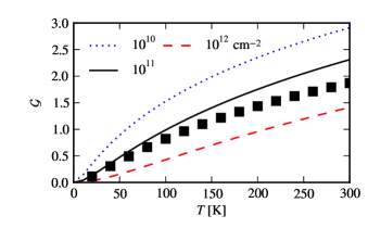
Figure 2: The dimensionless factor ${\cal G}$ in Eq. (15) as a function of charge density and temperature. Squares indicate results from Eq. (13) without further approximations (for $j=L$ and $n=10^{11}\,\mathrm{cm^{-2}}$).

The above results to the total power density

$${\cal J}_{j} \simeq N\frac{D_{1}^{2}\nu_{1}(\mu)^{2}}{\rho^{2}\alpha^{3}}k_{B}^{3}T^{2}\Delta T\frac{c_{j}D_{2}^{2}}{2\pi\hbar v_{F}^{2}\rho\alpha}{\cal G}(\frac{q_{c}}{q_{j,T}},\frac{k_{F}}{q_{j,T}})$$ (15)

$${\cal G}(a,b) \equiv\int_{0}^{\infty}\frac{\mathrm{d}x\,}{\epsilon_{r}(\frac{k_{F}x}{b})^{2}}\frac{\log\bigl{(}\frac{x}{a}+\frac{a}{x}\bigr{)}+1.3}{x^{2}+2a^{2}}\frac{x^{3}}{4\sinh^{2}(x/2)}\,.$$ (16)

Here, $q_{j,T}=k_{B}T/(\hbar{}s_{j})$ are the thermal phonon wave vectors, and $\Delta T=T_{e}-T_{\rm ac}$ is the temperature difference between electrons and acoustic phonons. The numerical factor in front of ${\cal G}$ is, taking $D_{2}=7\,\mathrm{eV}$, $d_{L}\equiv{}c_{L}D_{2}^{2}/(2\pi\hbar v_{F}^{2}\rho\alpha)\approx 0.008$ for longitudinal acoustic modes and $d_{T}\approx 0.003$ for transverse modes. Moreover ${\cal G}$ diverges logarithmically as $a\to 0$ and $b\to 0$, so that the total temperature dependence is $T^{2}\ln^{2}(T)\Delta T$. In the opposite limit $a\to\infty$ we have ${\cal G}(a,b)\sim{}a^{-2}$. For parameters of graphene, the ratio is $q_{c}/q_{L,T}\sim{}\sqrt{100\,\mathrm{K}/T}$, resulting to ${\cal G}$ of order 1 in the typical temperature range as illustrated in Fig. 2.

Mechanical strain in graphene also cuts off the $q^{2}$ behavior of the flexural phonon spectrum at low wave vectors. For isotropic relative strain $\tilde{u}$, one can find the corresponding result by replacing $q_{c}\mapsto{}q_{*}=\sqrt{\tilde{u}}s_{L}/\alpha$, which is of the order of $q_{c}$ for strains $\tilde{u}\sim{}10^{-4}$. Strain suppresses the flexural phonon mediated energy transport in a similar way as it suppresses the contribution to resistance. Castro et al. (2010)

For the acoustic phonon process $w^{L,T}$, we can find the supercollision energy transfer rate in a similar way:

$${\cal J} =2\pi N\frac{\nu_{1}^{2}D_{1}^{2}D_{2}^{2}}{2v_{F}^{2}\rho^{2}s_{L}s_{T}}\sum_{\gamma\gamma^{\prime}}\int_{0}^{\infty}\frac{\mathrm{d}q\,}{2\pi}\frac{qN^{el}_{\gamma\omega_{L,\mathbf{q}}+\gamma^{\prime}\omega_{T,\mathbf{q}}}}{\epsilon_{r}(q)^{2}}$$ (17)

$$\times(N_{\omega_{L,\mathbf{q}}}+\delta_{\gamma,+})(N_{\omega_{T,\mathbf{q}}}+\delta_{\gamma^{\prime},+})(\gamma\omega_{L,\mathbf{q}}+\gamma^{\prime}\omega_{T,\mathbf{q}})^{2}\,.$$

Neglecting screening and taking $s_{T}=0.67s_{L}$, we have

$${\cal J}_{LT} \approx 23N\frac{g^{2}\nu_{1}^{2}k_{B}^{3}T^{2}\Delta T}{\hbar}\frac{D_{2}^{2}k_{B}T}{\hbar^{2}v_{F}^{2}\rho s_{L}^{2}}\,,$$ (18)

Screening reduces the numerical prefactor roughly by a factor of $(1+4k_{F}/q_{L,T})^{-2}$.

Finally, for the processes involving optical phonons, a straightforward calculation for the transferred power density gives a result small compared to the direct 1-phonon process Bistritzer and MacDonald (2009).

IV Discussion

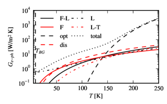
Figure 3: Thermal conductivity $G_{e-ph}={\cal J}/\Delta T$ between electrons and phonons, for monolayer graphene at charge density $n=10^{11}\,\mathrm{cm^{-2}}$, for parameter values given in the text. Several processes are shown: flexural-acoustic (F-L) multiphonon [Eq. (15)], acoustic-acoustic (L-T) [Eq. (18)], direct flexural phonon (F) [Ref. Song et al., 2012], optical phonons (opt) [Ref. Bistritzer and MacDonald, 2009], disorder-assisted supercollisions (dis) [Ref. Song et al., 2012, with $k_{F}\ell=200$], and acoustic phonons (L) [Ref. Kubakaddi, 2009; Viljas and Heikkilä, 2010]. Screening of deformation potential ($D_{1}=30\,\mathrm{eV}$) is in all processes taken into account as described in the text; this reduces the magnitude of the direct acoustic and flexural phonon processes, and slightly suppresses the others.

Similarly as for the resistance, the large population of the low-wavevector flexural phonons plays an important role for the flexural-acoustic phonon supercollisions. This is in contrast to the direct process, Song et al. (2012) in which the most relevant contribution comes from the thermal phonons with large wavevectors $q_{F,T}\gg{}q_{c},q_{*}$. Although scattering from low-wavevector flexural phonons occurs at a rapid rate, each event only transfers energy $\hbar\omega_{F,\mathbf{q}_{1}}+\hbar\omega_{F,\mathbf{q}_{2}}$. In contrast, a supercollision scattering event involving phonons of similar wave vectors transfers a significantly larger energy $\hbar\omega_{L,\mathbf{q}}$. This partly compensates for the smaller matrix elements.

The energy flow for the direct flexural phonon process is Song et al. (2012)

$${\cal J}_{\rm flex}=0.12N\frac{[D_{1}(2k_{F})^{2}+D_{2}^{2}]\nu_{1}(\mu)^{2}}{\rho^{2}\alpha^{3}}k_{B}^{3}T^{2}\Delta T\,,$$ (19)

where the screening of the deformation potential is taken into account within the same model as above. Comparing this to the multiphonon process discussed above, with the parameter values discussed in Sec. II, we find ${\cal J}_{L}\sim{}{\cal J}_{\rm flex}$. If screening is neglected, we have instead ${\cal J}_{L}\sim 0.1{\cal J}_{\rm flex}$. The comparison to the direct flexural and the disorder-assisted process is shown in Fig. 3. The multiphonon process can be of a similar order of magnitude as the disorder-assisted one in very clean samples.

Several parameters in Eq. (15) can be obtained by a comparison to a resistivity measurement, in which flexural phonons in the parameter regime relevant here contribute a $T^{2}$ increase. Castro et al. (2010); Mariani and von Oppen (2010) In particular, assuming weak strain, $k_{F},q_{*}\ll{}q_{F,T}$, one can rewrite Eq. (15) in terms of the resistivity contribution $\rho_{F}\propto{}T^{2}$ expected to originate from flexural phonons: Castro et al. (2010); Mariani and von Oppen (2010); Ochoa et al. (2011)

$${\cal J}_{L} \approx 100\frac{g^{2}\nu_{1}^{2}k_{B}^{3}T^{2}\Delta T}{\hbar}\frac{4e^{2}\rho_{F}}{h}\begin{cases}\frac{q_{*}^{2}{\cal G}}{q_{L,T}^{2}}\,,&\text{$k_{F}\ll{}q_{*}$,}\\ \frac{k_{F}^{2}{\cal G}}{q_{L,T}^{2}\ln\frac{q_{F,T}}{q_{c}}}\,,&\text{$q_{*}\ll{}k_{F}$,}\end{cases}$$ (20)

where $g^{2}=D_{1}^{2}/(2\rho s_{L}^{2})$. The electron-phonon coupling $\tilde{D}$ in the resistivity in principle also contains the deformation potential, but under the screening assumptions here and using the parameter values quoted above (which are those used in Ref. Castro et al., 2010), we approximated $\tilde{D}\approx{}D_{2}$. What can be seen in Eq. (20) is that an effective $k_{F}\ell$ inferred from the resistance for flexural phonons must be adjusted for the difference in the characteristic phonon wave vector scales: $\max(k_{F},q_{*})$ for resistance and $q_{L,T}$ for supercollisions. For the acoustic phonon process, we can find a relation to the resistance contribution in a similar way: $(D_{2}^{2}k_{B}T)/(\hbar^{2}v_{F}^{2}\rho s_{L}^{2})\approx(4e^{2}\rho_{L/T})/h$ (cf. e.g. Ref. Ochoa et al., 2011).

Flexural phonons are thermally induced dynamic ripples in graphene, and as far as quasielastic scattering is concerned, the physics is similar to the case of static ripples. Indeed, the function ${\cal Y}(\mathbf{q})$ in Eq. (14) above is closely related to the correlation function of out-of-plane displacements that appears in the case of static ripples. Katsnelson and Geim (2008) Supercollision scattering from static ripples was considered in Ref. Song et al., 2011, assuming small-scale ripples with characteristic wave vector $q_{c}\gg{}q_{L,T},k_{F}$, and a temperature-independent amplitude $Z$ chosen larger than the effective thermal ripple size in the above flexural phonon calculation. Interestingly, this also results to a $T^{2}\Delta T$ temperature dependence, but originating from the $a^{-2}$ scaling of ${\cal G}$. The magnitude of the effect is sensitive to the amplitude of the ripples: different experimental parameters Lundeberg and Folk (2010); Song et al. (2011) lead to $k_{F}\ell_{\rm{}eff}\sim{}a^{2}/q_{c}^{2}Z^{4}=10^{0}\ldots 10^{4}$. The amplitude and characteristic length scale of ripples is in principle visible also in the resistivity. Katsnelson and Geim (2008)

Finally, we can point out that electron–phonon processes in bilayer graphene have similar phase space restrictions as in monolayer. Supercollision and multiphoton processes are possible also there, and have the advantage that due to the quadratic Hamiltonian, the two terms in Eq. (7) have the same sign, so that the selection rules are less strict. However, the magnitude of the effect is also reduced, because the quadratic spectrum implies that the virtual electron state involved lies at a higher energy. This gives more weight to small $q$-values, which implies that screening will be of importance.

In summary, I discussed the effect of multiphonon processes on the energy transport in monolayer graphene at intermediate temperatures. I find that in ultraclean suspended graphene samples, multiphonon processes arising in second order of perturbation theory can compete in the energy flow over first-order acoustic and flexural phonon processes and disorder-assisted supercollisions. However, these results are sensitive to the electronic screening, mechanical strain, and non-thermal ripples in the system.

I thank P. Hakonen and T.T. Heikkilä for useful discussions. This work was supported by the Academy of Finland.

References

Song et al. (2012)
J. C. W. Song,
M. Y. Reizer,
and L. S.
Levitov, Phys. Rev. Lett.
109, 106602
(2012).
Betz et al. (2013)
A. C. Betz,
S. H. Jhang,
E. Pallecchi,
R. Feirrera,
G. Fève,
J.-M. Berroir,
and
B. Plaçais,
Nat. Phys. 9,
109 (2013).
Chen and Clerk (2012)
W. Chen and
A. A. Clerk,
Phys. Rev. B 86,
125443 (2012).
Song et al. (2011)
J. C. W. Song,
M. Y. Reizer,
and L. S.
Levitov (2011),
arXiv:1111.4678v1.
Bolotin et al. (2008)
K. I. Bolotin,
K. J. Sikes,
J. Hone,
H. L. Stormer,
and P. Kim,
Phys. Rev. Lett. 101,
096802 (2008).
Castro et al. (2010)
E. V. Castro,
H. Ochoa,
M. I. Katsnelson,
R. V. Gorbachev,
D. C. Elias,
K. S. Novoselov,
A. K. Geim, and
F. Guinea,
Phys. Rev. Lett. 105,
266601 (2010).
Mariani and von Oppen (2008)
E. Mariani and
F. von Oppen,
Phys. Rev. Lett. 100,
076801 (2008).
Guinea et al. (2008)
F. Guinea,
B. Horovitz, and
P. Le Doussal,
Phys. Rev. B 77,
205421 (2008).
Morozov et al. (2006)
S. V. Morozov,
K. S. Novoselov,
M. I. Katsnelson,
F. Schedin,
L. A. Ponomarenko,
D. Jiang, and
A. K. Geim,
Phys. Rev. Lett. 97,
016801 (2006).
Zakharchenko et al. (2010)
K. V. Zakharchenko,
R. Roldán,
A. Fasolino, and
M. I. Katsnelson,
Phys. Rev. B 82,
125435 (2010).
Bistritzer and MacDonald (2009)
R. Bistritzer and
A. H. MacDonald,
Phys. Rev. Lett. 102,
206410 (2009).
Ochoa et al. (2011)
H. Ochoa,
E. V. Castro,
M. I. Katsnelson,
and F. Guinea,
Phys. Rev. B 83,
235416 (2011).
Bruus and Flensberg (2004)
H. Bruus and
K. Flensberg,
Many-Body Quantum Theory in Condensed Matter Physics:
An Introduction (Oxford University Press,
2004).
Kubakaddi (2009)
S. S. Kubakaddi,
Phys. Rev. B 79,
075417 (2009).
Viljas and Heikkilä (2010)
J. K. Viljas and
T. T. Heikkilä,
Phys. Rev. B 81,
245404 (2010).
Mariani and von Oppen (2010)
E. Mariani and
F. von Oppen,
Phys. Rev. B 82,
195403 (2010).
Katsnelson and Geim (2008)
M. I. Katsnelson
and A. K. Geim,
Phil. Trans. R. Soc. A 366,
195 (2008).
Lundeberg and Folk (2010)
M. B. Lundeberg
and J. A. Folk,
Phys. Rev. Lett. 105,
146804 (2010).