Heater self-calibration technique for shape prediction of fiber tapers

Abstract

In the production of tapered optical fibers, it is important to control the fiber shape according to application-dependent requirements and to ensure adiabatic tapers. Especially in the transition regions, the fiber shape depends on the heater properties. The axial viscosity profile of the fiber within the heater can, however, be hard to access and is therefore often approximated by assuming a uniform temperature distribution. We present a method for easy experimental calibration of the viscosity profile within the heater. This allows the determination of the resultant fiber shape for arbitrary pulling procedures, using only an additional camera and the fiber drawing setup itself. We find very good agreement between the modeled and measured fiber shape.

I Introduction

During the past decade the amazing properties of tapered optical fibers (TOFs), such as low losses and the possibility to concentrate large intensities in an evanescent light field, have been extensively explored. They are now applied in various fields ranging from optical bio-sensing to quantum optics [1, 2, 3, 4, 5, 6, 7]. In bio-sensing, TOFs with biorecognition molecules in the evanescent field area [8] enable the detection of specific target molecules; in quantum optics, the high single-photon field strength near the fiber surface allows for quantum light-atom interfaces employing only a few atoms[9, 10].

A TOF is produced by heating a section of commercial optical fiber while pulling its ends apart. Tailoring of the taper shape, such that it fulfills the adiabaticity criteria[11, 12], is important to avoid coupling light from the fundamental mode to higher-order and radiation modes.

Traditionally, the tapered shape is modeled by assuming a uniform viscosity profile of the heated fiber such that it is infinite outside the heated section and finite inside [13, 14, 15]. From measured shapes we find that this simplified approach is not sufficient for TOFs produced in a microheater, as both the waist and the shape of the tapers are not predicted correctly. The resulting shape of the TOF inherently depends on the strongly temperature-dependent viscosity profile of the fiber induced by the heating device. While in flame-brushing fiber processing [16] the effective temperature distribution can be relatively uniform, for heaters where this approximation fails, it is necessary to include a fluid-dynamical description of the fiber flow during the pulling procedure (given in Sec. III-B).

Furthermore, we have confirmed that the fiber flow not only depends on the applied boundary conditions of the pulling procedure, but also on the momentary shape of the heat-softened fiber. This was also observed in [17], where the authors characterize their heater and heuristically include its properties in a fiber-shape model.

In this work, we present a fluid-dynamics based model for the TOF shape, taking into account both the axially varying viscosity profile and the momentary shape-dependency of the axial velocity profile.

We provide a practical method to calibrate the parameters of the heater via simple data analysis of the measured shape of a single TOF made for this purpose. This calibration allows us to predict precisely the shape of TOFs manufactured with arbitrary pulling procedures.

II Experimental setup

II-A Fiber-pulling rig

To produce a TOF we use a fiber-pulling rig consisting of two stacked motorized linear translation stages and an NTT CMH-7019 electric ceramic microheater (oven), as illustrated in Fig. 1. The stacked solution of the stages provides improved stability compared to stages placed in succession of each other [18]. By only moving the bottom stage, the fiber can easily be translated (without stretching it) with respect to the stationary oven. During a pull, the bottom stage moves one end of the fiber with velocity $v_{+}$, whereas the combined motion of the top and bottom stages moves the other end with velocity $v_{-}$. In this paper we restrict ourselves to cases where $v_{+}-v_{-}>0$, i.e., where the fiber is never compressed.

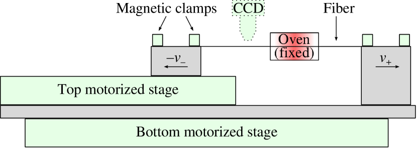
Figure 1: Schematic drawing of the fiber-pulling rig. The CCD camera is only inserted after the pulling procedure when the oven has been removed from the setup.

Driving the oven with electrical heating powers ranging from 97-103 W, we reproducibly observe identical TOF shapes. We also confirm that the resultant shape only depends on the ratio of the pull speeds $v_{+}/v_{-}$, rather than on their value, as long as the speeds are sufficiently low that the fiber does not slip underneath the magnetic clamps. This is a consequence of Newtonian fluid flow, and (for a slow quasi-static pull) the fiber shape therefore only depends on the pull lengths on either side of the oven.

II-B Imaging

To measure the TOF shape we image it with a CCD camera through a $25\times$ microscope objective placed above the fiber (Fig. 1). The imaging is non-destructive, fast, and in situ: we obtain the full fiber shape by repeatedly recording an image and translating the TOF with the bottom stage. The individual images are joined, and a typical example of 300 merged images is shown in Fig. 2a. The green dashed curves indicate the fiber edges found by an edge-detection algorithm: for each image column, we calculate the convolution with a template kernel. We locate the position of the edges by the outermost local minimum/maximum values of the convolution that are significant enough to exceed a threshold level, as indicated in Fig. 2b. Introducing this threshold prevents detection errors caused by the narrow, bright features close to the fiber axis; its value is set to $25\%$ of the extremal convolution values found in the unstretched fiber. As template kernel we use the derivative of a Gaussian with a width chosen such that the kernel models the pixel values observed at the edges of the unstretched fiber.

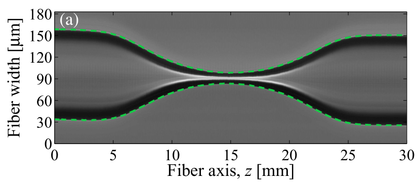
(a)

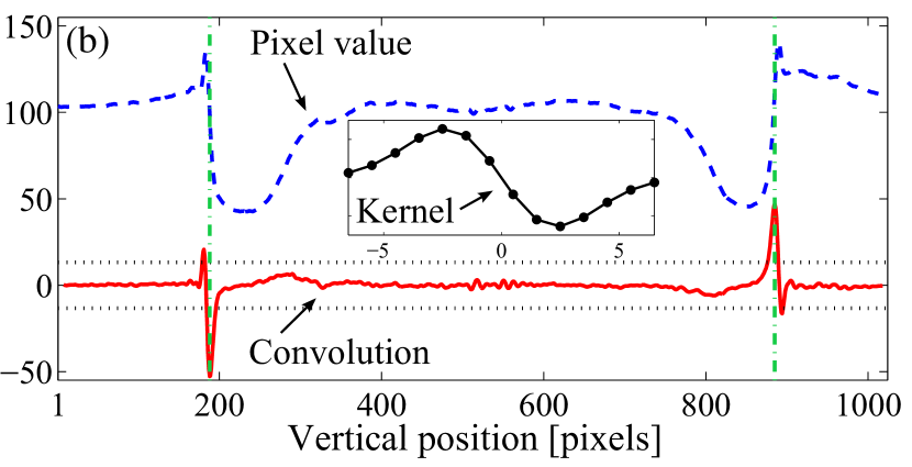
(b)

Figure 2: (a) 300 joined CCD images of a TOF, symmetrically elongated by $l=15\,\mathrm{mm}$. The waist is measured to $d_{\text{w}}=15\,\mathrm{\mu m}$. The aspect ratio is not to scale. (b) Edge-detection algorithm. Dashed blue line: Pixel values along the image column at $z=5\,\mathrm{cm}$. Solid red line: Convolution. Dotted black lines: Threshold levels ($=\pm 13$). Dashed-dotted green lines: Located edge positions. Inset: Edge-detection kernel.

We estimate the precision of the diameter detection in two ways. Determining the fiber diameter of an unstretched $125\,\mathrm{\mu m}$ fiber at $10^{5}$ image columns, we obtain a fiber width of $694\,\mathrm{pixels}$ with a $1\,\mathrm{pixel}$ uncertainty in every column. Additionally, after stretching the fiber by $15\,\mathrm{mm}$, we observe only a relative change of the fiber volume $<10^{-3}$ compared to the unstretched fiber. The dominating contribution to the uncertainty is given by how well the diameter of the unstretched fiber is known.

Because the edge detection is limited by the optical imaging resolution, diffraction effects, and the fiber bending out of the focal plane, only TOFs with waist diameters larger than $\approx 10\,\mathrm{\mu m}$ can be measured. We confirm the validity of our model also for thinner TOFs by additionally using a scanning electron microscope (SEM) to measure the diameter at selected axial positions, as shown in Fig. 3. The SEM imaging is not necessary for the presented calibration method, it is merely used for verification.

Figure 3: Comparison of fiber-diameter measuring methods. At several selected positions the fiber diameter is determined both using the CCD imaging and the SEM. For fiber diameters $<10\,\mathrm{\mu m}$ diffraction effects limit the accuracy of the CCD method (indicated by the dashed lines), whereas the SEM method fails for large fibers due to space-charge buildup.

III Modeling the fiber shape

We consider an optical fiber with position- and time-dependent cross-sectional area $A(z,t)$ passing through a heater, as illustrated in Fig. 4.

III-A Boundary conditions

The axial fiber flow $v(z,t)$, at position $z$ and time $t$ for regions on either side of the heated section corresponds to the speed of the respective fiber holders:

$$v(z,t) =v_{-},\quad\text{for }z<z_{-}\,,$$ (1a)

$$v(z,t) =v_{+},\quad\text{for }z>z_{+}\,,$$ (1b)

where the sign of $v_{\pm}$ follows the direction of the pull. Inside the heated zone, $v(z,t)$ is described by an unknown function that depends on the pull speeds, the momentary fiber shape, and the axial viscosity distribution of the fiber, resulting from the axial temperature profile of the heater (neglecting any transverse variation).

Figure 4: Boundary conditions during the fiber pulling procedure. $l_{\pm}=v_{\pm}t=\tilde{z}_{\pm}-z_{\pm}$ are the elongated lengths of the fiber on either side of the heated section represented by the red area in the center.

The boundary between each taper and the unstretched fiber is denoted by $\tilde{z}_{\pm}$. Outside the tapered sections ($z<\tilde{z}_{-}$ or $z>\tilde{z}_{+}$), the cross-sectional area corresponds to that of the initially uniform fiber, $A(z,t)=A_{0}$. We introduce the following abbreviations:

$$v_{\infty} \equiv v_{+}-v_{-}\, \text{denotes the stretching speed},$$ (2a)

$$A_{\text{n}}(z,t) \equiv\frac{A(z,t)}{A_{0}}\, \text{the normalized cross-sectional area}.$$ (2b)

III-B Fiber shape

The evolution of the fiber shape during the tapering procedure can be described by two coupled differential equations for the normalized cross-sectional area $A_{\text{n}}(z,t)$ and the axial velocity profile of the fiber $v(z,t)$ [19, 15]. The continuity equation

$$\frac{\partial}{\partial t}A_{\text{n}}(z,t)+\frac{\partial}{\partial z}\Big{(}A_{\text{n}}(z,t)\,v(z,t)\Big{)}=0\,$$ (3)

governs mass conservation, and a simplified equation describes axial momentum conservation:

$$\frac{\partial}{\partial z}\Big{(}\eta(z)A_{\text{n}}(z,t)\frac{\partial}{\partial z}v(z,t)\Big{)}=0\,,$$ (4)

where $\eta(z)$ is the axial viscosity of the fiber fluid. Equation (4) is derived by solving the Navier-Stokes equations for an axisymmetric incompressible Newtonian fluid in the limit of Stokes flow, neglecting body forces (such as gravity, which is negligible compared to viscous forces), and by Taylor-expanding the equations to lowest order in the radial variable [20]. The fiber is thin, and its heat conductivity is poor compared to that of the much bigger surrounding oven. Therefore the temperature along the fiber (and hence $\eta(z)$) is a function of the axial position within the oven alone. Additionally, we ensure that each mass element of the fiber is in thermal equilibrium with the surroundings by asserting slow motion of the fiber.

In order to solve (3) and (4) numerically, it is necessary to know $\eta(z)$. Often, this is simply approximated by a uniform distribution such that it is infinite outside the heated region of the fiber and finite and constant inside [15, 13, 14]. Xue et al. [21] measure the temperature distribution of their heater and use the Arrhenius model for the viscosity dependence on the temperature to indirectly deduce $\eta(z)$. Pricking et al. [17] heuristically model $\eta(z)$ by a flattened Gaussian profile. In the following we show how $\eta(z)$ instead can be easily inferred experimentally by measuring the resultant fiber shape after a short symmetric ($-v_{-}=v_{+}$) pull. We thereby avoid cumbersome temperature-viscosity calibrations and measurements of the temperature profile inside the heater.

III-C Fiber fluidity

Since the TOF shape depends on the ratio of the velocities, and not on the individual velocities, only a dependence on the pull lengths $l_{\pm}=v_{\pm}t$ remains. It is therefore more convenient and intuitive to express the following equations in terms of the total elongation length

$$l=l_{+}-l_{-}=v_{\infty}t$$ (5)

instead of time, such that $v(z,t)\rightarrow v(z,l)$ and $A_{\text{n}}(z,t)\rightarrow A_{\text{n}}(z,l)$.

Integrating (4) over $z$ yields

$$\eta(z)A_{\text{n}}(z,l)\frac{\partial}{\partial z}v(z,l)=C(l);$$ (6)

the integration constant $C(l)$ does not depend on $z$. We solve (6) for $\frac{\partial}{\partial z}v(z,l)$ and integrate over $z$ again, starting at an arbitrary position $z_{0}$, and obtain

$$v(z,l)=v(z_{0},l)+v_{\infty}\cdot\frac{\int_{z_{0}}^{z}\frac{\tau(\zeta)}{A_{\text{n}}(\zeta,l)}\,\mathrm{d}\zeta}{\int_{z_{-}}^{z_{+}}\frac{\tau(\zeta)}{A_{\text{n}}(\zeta,l)}\,\mathrm{d}\zeta}\,,$$ (7)

for the axial velocity profile. The integration constant

$$C(l)=\frac{v_{\infty}}{\int_{z_{-}}^{z_{+}}\frac{1}{\eta(\zeta)A_{\text{n}}(\zeta,l)}\,\mathrm{d}\zeta}$$ (8)

has been fixed by requiring continuity at the boundaries $v(z_{\pm},l)=v_{\pm}$; we also introduced the normalized fiber fluidity:

$$\tau(z)=\frac{\frac{1}{\eta(z)}}{\int_{-\infty}^{\infty}\frac{1}{\eta(\zeta)}\,\mathrm{d}\zeta}\,.$$ (9)

Please note that $\tau(z)$ only differs from zero inside the heated section bounded by $z_{\pm}$.

III-D Short pull

In the following, we consider a symmetric pull where the fiber elongation length $l$ is much smaller than the heated section. In this limit, the spatial variation of the normalized fiber cross-sectional area $A_{\text{n}}(z,l)$ over regions with non-zero $\tau(z)$ can be neglected and (7), describing the axial velocity profile, simplifies significantly. If $z_{0}$ is chosen outside the heat-softened section, such that $v(z_{0},l)$ is constant, we find

$$v(z,l)\approx v(z)=v(z_{0})+v_{\infty}\int_{z_{0}}^{z}\tau(\zeta)\,\mathrm{d}\zeta$$ (10)

to be constant in $l$ during the whole pulling process. From this, the fiber fluidity can be readily approximated by

$$\tau(z)\approx\frac{\mathrm{d}}{\mathrm{d}z}\frac{v(z,l)}{v_{\infty}}\,.$$ (11)

Since the axial velocity profile is now independent of the elongation length, the continuity equation (3) can be solved analytically to yield an explicit form for the normalized fiber cross-sectional area:

$$A_{\text{n}}(z,l) =\frac{\partial}{\partial z}\Bigl{(}q^{-1}\bigl{(}q(z)-l\bigr{)}\Bigr{)}$$ (12a)

$$\text{with }q(z) \equiv\int_{z_{*}}^{z}\frac{v_{\infty}}{v(\zeta)}\,\mathrm{d}\zeta\,,$$ (12b)

as can be directly verified by differentiation, i.e., by inserting (12a) and (12b) into (3). $q^{-1}(\cdot)$ denotes the inverse function of $q(z)$, and $z_{*}$ is an arbitrarily chosen position. We integrate both sides of (12a) from $\tilde{z}_{\pm}$ and define a new variable

$$y(z,l) \equiv q^{-1}\big{(}q(z)-l\big{)}\text{, so that}$$ (13a)

$$y(z,l) =\int_{\tilde{z}_{\pm}}^{z}A_{\text{n}}(\zeta,l)\,\,\mathrm{d}\zeta\,+z_{\pm}.$$ (13b)

The second term in (13b) follows from choosing $z_{*}=z_{\pm}$ in (12b). The expression $z-y(z,l)$ can be interpreted as the distance that a fiber volume element at position $z$ has moved during the pulling process.

We apply $q(\cdot)$ to both sides of (13a) and differentiate with respect to $z$. Using (13b) to express $\frac{\partial y}{\partial z}$ and (12b) to express $\frac{\mathrm{d}q}{\mathrm{d}z}$ in the result, we obtain a recursion formula for the axial velocity profile of the fiber:

$$v\bigl{(}y(z,l)\bigr{)}=A_{\text{n}}(z,l)\,v(z)\,.$$ (14)

Both $A_{\text{n}}(z,l)$ and $y(z,l)$ are known from the fiber shape measurements (the latter via  (13b)). On the left side of the oven $y(z,l)>z$. Starting from $z=\tilde{z}_{-}$, using (14), we can now calculate $v(y(z,l))$ from $v(z)$, which lies further to the left, until $y(z,l)$ approaches $z$. The same can be done from the other side starting from $z=\tilde{z}_{+}$, since there $y(z,l)<z$.

The following pseudo-code illustrates the algorithm for calculating $v(z)$ in the interval $[\tilde{z}_{-},\tilde{z}_{+}]$ with a step size $\Delta z>0$:

1:vz${}_{\text{table}}\leftarrow\big{\{}(v_{-},\tilde{z}_{-}),\,(v_{+},\tilde{z}_{+})\big{\}};$

2:$z\leftarrow\tilde{z}_{-};\quad v\leftarrow v_{-};\quad y\leftarrow\tilde{z}_{-}-l_{-};$

3:while $y>z$ do

4:     insert $\big{(}v\cdot A_{\text{n}}(z),y\big{)}$ into $\text{vz}_{\text{table}};$

5:     $z\leftarrow z+\Delta z;$

6:     $y\leftarrow y+\Delta z\cdot A_{\text{n}}(z);$

7:     $v\leftarrow\texttt{interpolate}(\text{vz}_{\text{table}},z);$

8:end while;

9:$z\leftarrow\tilde{z}_{+};\quad v\leftarrow v_{+};\quad y\leftarrow\tilde{z}_{+}-l_{+};$

10:while $y<z$ do

11:     insert $\big{(}v\cdot A_{\text{n}}(z),y\big{)}$ into $\text{vz}_{\text{table}};$

12:     $z\leftarrow z-\Delta z;$

13:     $y\leftarrow y-\Delta z\cdot A_{\text{n}}(z);$

14:     $v\leftarrow\texttt{interpolate}(\text{vz}_{\text{table}},z);$

15:end while;

In this way the complete velocity profile $v(z)$ is contained in $\text{vz}_{\text{table}}$, and by (11) the fiber fluidity can be calculated.

IV Results

IV-A Calibration

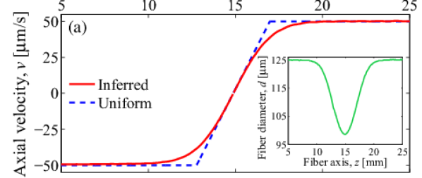
(a)

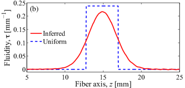
(b)

Figure 5: (a) Axial velocity profile. Inset: measured fiber diameter of an $l=2\,\mathrm{mm}$ stretched fiber used to infer $v(z,l)$. (b) Axial fluidity profile, inferred by applying (11) to (a). Red solid lines depict data inferred with the presented algorithm. Blue dashed lines depict data corresponding to a uniform fluidity profile with $L_{0}=4.2\,\mathrm{mm}$, which results in an identical waist diameter.

To the measured shape $d(z,l)=2\sqrt{A(z,l)/\pi}$ of a TOF which was elongated symmetrically by $l=2\,\mathrm{mm}$ with speeds $v_{\pm}=\pm 50\,\mathrm{\mu m/s}$, we apply the recursion formula (14) to infer the axial velocity profile $v(z,l)$ shown in Fig. 5a. Also depicted is a simplifying model which was introduced in the seminal paper by Birks and Li [13]. It is commonly used to describe flame-brushing fiber processing [16], and it approximates $v(z)$ inside the heated section by interpolating linearly between the exterior pull velocities $v_{\pm}$ over an “effective hot-zone length” $L_{0}=\left.v_{\infty}/\frac{\,\mathrm{d}v}{\,\mathrm{d}z}\right|_{v=0}$.

The effective hot-zone length $L_{0}$ can be found from the waist diameter $d_{\text{w}}$ using Birks’ and Li’s formula:

$$d_{\text{w}}(l)=d_{0}\exp{\bigg{(}-\frac{l}{2L_{0}}\bigg{)}}\,.$$ (15)

To calibrate $\eta(z)$, we use a TOF with an initial diameter $d_{0}=125\,\mathrm{\mu m}$ and a final waist diameter $d_{\text{w}}=98\,\mathrm{\mu m}$, which results in $L_{0}=4.2\,\mathrm{mm}$.

The curves for $v(z)$ in Fig. 5a agree in value and slope at the oven center and at the ends by construction but they deviate substantially at the edges of the heated section. The difference is even more pronounced in $\tau(z)$, which is depicted in Fig. 5b. This strongly suggests that the assumption of a uniform temperature distribution does not describe our setup.

IV-B Modeling a symmetric pull

Given the inferred fiber fluidity $\tau(z)$ we numerically solve the system of equations (3) and (7), using the MATLAB function ode45 with a relative error tolerance of $10^{-6}$. For thin TOFs with diameters below $\approx 1\,\mathrm{\mu m}$, numerical instabilities can occur, which necessitates decreasing the relative and absolute error tolerances further. Alternatively, by adding a term $D\frac{\partial^{2}A_{\text{n}}(z,t)}{\partial z^{2}}$ to the right-hand side of (3), using a small “diffusion coefficient” $D$ such that $2\sqrt{Dl/v_{\infty}}\ll L_{0}$, we can effectively eliminate the numerical stiffness of the problem without introducing a significant change to the solution.

In Fig. 6, we present the modeling of four symmetrically stretched fibers, which were elongated by $l=5,10,15,20\,\mathrm{mm}$ with speeds $v_{\pm}=\pm 50\,\mathrm{\mu m/s}$. We observe very good agreement between the measured and modeled diameter with only a $1\%$ discrepancy at the waist of the $l=5\,\mathrm{mm}$ and $l=10\,\mathrm{mm}$ streched fibers, and $2\%$ for the $l=15\,\mathrm{mm}$ fiber. For the longer $l=20\,\mathrm{mm}$ stretched fiber the discrepancy is 13%; however, here the waist is so thin, $d_{\text{w}}\approx 6\,\mathrm{\mu m}$, that the CCD imaging starts to fail.

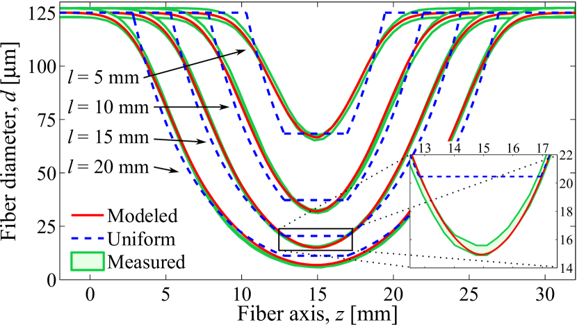
Figure 6: Fiber diameter of four different symmetrically pulled fibers with various elongation lengths $l$. Solid red line: Model. Green lines enclosing shaded area: Fiber diameter as measured with CCD camera with measurement uncertainty. Dashed blue line: Fiber shape prediction using an $L_{0}=4.2\,\mathrm{mm}$ uniform fluidity profile. The inset shows a zoom of the waist of the fiber stretched by $l=15\,\mathrm{mm}$.

For reference, we also show the predicted TOF shape using a uniform profile for the fluidity with $L_{0}=4.2\,\mathrm{mm}$, which (by definition) predicts the waist correctly for $l=2\,\mathrm{mm}$. For this $\tau(z)$ it is evident that the waist size is increasingly overestimated for longer pull lengths. As can also be observed by numerically solving (4), this implies that the effective hot-zone length $L_{0}$ (15) of the fiber shrinks during the pull (i.e., for smaller fiber diameters) in agreement with similar observations made in [17]. This shape-dependency makes it impossible to predict the waist for arbitrary pull lengths using a constant-width box-profile for the fluidity, as it fails to reproduce qualitative features of the TOF shape. Especially the prediction of a homogeneous waist with length $L_{0}$ is absent in the data. This necessitates non-symmetric pulling procedures for producing TOFs with long homogeneous waists.

In Fig. 7, for symmetric pulls, we compare the predicted fiber waist diameter resulting from our calibration method with experimental data and the simplified prediction (15). Whereas the latter overestimates the waist for longer pull lengths, our simulations display good agreement with the data even for very thin TOFs, where the initial diameter has been reduced by a factor of 250 from $125\,\mathrm{\mu m}$ to about $500\,\mathrm{nm}$.

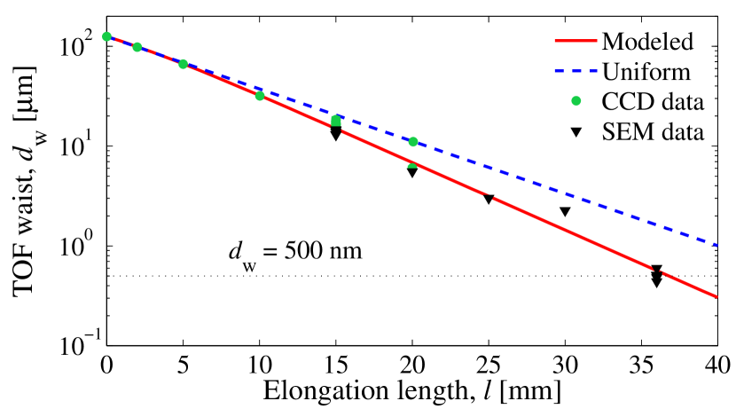
Figure 7: TOF waist of symmetrically elongated fibers. Note the log scale on the y-axis.

In trying to fit (15) to the data shown in Fig. 7 by determining an effective $L_{0}$ [16, 22, 23], one would compromise on the predicted corresponding shape of the tapers instead.

IV-C Modeling an asymmetric pull

The fiber shape model presented here is not only restricted to symmetric pulls, where $-v_{-}=v_{+}$, but can be applied to any combination of pull speeds. This is extremely useful as it makes it possible to test various pulling procedures without actually performing them.

Here we show the extreme situation where the two fiber ends are moved in the same direction such that the fiber is being pushed into the oven from one side while being pulled out on the other side with a greater speed, i.e., $0<v_{-}<v_{+}$. The measured and modeled diameter of such an asymmetrically pulled TOF is shown in Fig. 8. Here, an elongation of 15 mm is obtained by push and pull speeds $v_{-}=10\,\mathrm{\mu m/s}$ and $v_{+}=100\,\mathrm{\mu m/s}$. The modeled curve predicts the data very closely with only a 3% discrepancy at the waist and well within the uncertainty of the CCD data.

We demonstrate that especially in a situation where the axial fiber diameter changes strongly within the heated zone, accurate modeling of the viscosity profile leads to a significant improvement of the fiber shape prediction.

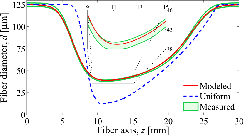
Figure 8: Shape of a TOF, asymmetrically elongated by $l=15\,\mathrm{mm}$. Red solid line: Predicted fiber shape using the inferred fluidity profile depicted in Fig. 5. Green lines enclosing shaded area: CCD measured diameter. Blue dashed line: Solution to (3) and (7) using a uniform fluidity profile with $L_{0}=4.2\,\mathrm{mm}$. The inset shows a zoom of the fiber waist.

V Conclusion

We present a general fiber shape model applicable to arbitrary pulling procedures. Crucial for the model is the fluidity profile of the fiber provided by the heater. We show how this can be inferred experimentally using the fiber-pulling apparatus itself, assuming only a temperature profile inside the oven that does not depend on the fiber shape. The experimental calibration of the heater properties allows a precise numerical prediction of the fiber shape. We thus expect our method to facilitate the design of pulling procedures for a wide range of applications requiring precision control of the fiber shape. These include manufacturing of fiber-couplers and tapered optical nanofibers for atom traps and nano-photonics. Whereas the method presented here only allows one to predict precisely the shape of the TOF for a given pulling procedure, the inverse problem is of central interest for production of TOFs. In the case that a uniform fluidity profile describes the physics sufficiently well, algorithms to approximate the intended fiber shape do exist[14]. Using such a solution as a starting point, the proposed method could be used to solve a variational optimization problem, adapting trial pulling procedures to regimes where other algorithms fail. We are currently working on implementing this approach.

References

- [1] V. I. Balykin, K. Hakuta, F. Le Kien, J. Q. Liang, and M. Morinaga, “Atom trapping and guiding with a subwavelength-diameter optical fiber,” Phys. Rev. A, vol. 70, no. 1, p. 011401, Jul. 2004.
- [2] Y. Xiao, C. Meng, P. Wang, Y. Ye, H. Yu, S. Wang, F. Gu, L. Dai, and L. Tong, “Single-nanowire single-mode laser,” Nano Lett., vol. 11, no. 3, pp. 1122–1126, Mar. 2011.
- [3] R. Garcia-Fernandez, W. Alt, F. Bruse, C. Dan, K. Karapetyan, O. Rehband, A. Stiebeiner, U. Wiedemann, D. Meschede, and A. Rauschenbeutel, “Optical nanofibers and spectroscopy,” Appl. Phys. B, vol. 105, no. 1, pp. 3–15, Sep. 2011.
- [4] T. Lee, Y. Jung, C. A. Codemard, M. Ding, N. G. R. Broderick, and G. Brambilla, “Broadband third harmonic generation in tapered silica fibres,” Opt. Express, vol. 20, no. 8, p. 8503, Apr. 2012.
- [5] Y.-S. Park and H. Wang, “Resolved-sideband and cryogenic cooling of an optomechanical resonator,” Nat. Phys., vol. 5, no. 7, pp. 489–493, Jun. 2009.
- [6] G. Bahl, K. H. Kim, W. Lee, J. Liu, X. Fan, and T. Carmon, “Brillouin cavity optomechanics with microfluidic devices,” Nat. Commun., vol. 4, pp. 1–6, Jun. 2013.
- [7] M. Sumetsky, Y. Dulashko, J. M. Fini, A. Hale, and D. J. DiGiovanni, “The microfiber loop resonator: Theory, experiment, and application,” J. Lightwave Technol., vol. 24, no. 1, pp. 242–250, Jan. 2006.
- [8] X. Fan, I. M. White, S. I. Shopova, H. Zhu, J. D. Suter, and Y. Sun, “Sensitive optical biosensors for unlabeled targets: A review,” Anal. Chim. Acta, vol. 620, no. 1-2, pp. 8–26, Jul. 2008.
- [9] D. J. Alton, N. P. Stern, T. Aoki, H. Lee, E. Ostby, K. J. Vahala, and H. J. Kimble, “Strong interactions of single atoms and photons near a dielectric boundary,” Nat. Phys., vol. 7, no. 2, pp. 159–165, Nov. 2010.
- [10] E. Vetsch, D. Reitz, G. Sagué, R. Schmidt, S. T. Dawkins, and A. Rauschenbeutel, “Optical interface created by laser-cooled atoms trapped in the evanescent field surrounding an optical nanofiber,” Phys. Rev. Lett., vol. 104, no. 20, p. 203603, May 2010.
- [11] J. D. Love and W. M. Henry, “Quantifying loss minimisation in single-mode fibre tapers,” Electron. Lett., vol. 22, no. 17, pp. 912–914, Aug. 1986.
- [12] J. D. Love, W. M. Henry, W. J. Stewart, R. J. Black, S. Lacroix, and F. Gonthier, “Tapered single-mode fibres and devices. i. adiabaticity criteria,” IEE Proc-J, vol. 138, no. 5, pp. 343–354, Oct. 1991.
- [13] T. A. Birks and Y. W. Li, “The shape of fiber tapers,” J. Lightwave Technol., vol. 10, no. 4, pp. 432–438, Apr. 1992.
- [14] C. Baker and M. Rochette, “A generalized heat-brush approach for precise control of the waist profile in fiber tapers,” Opt. Mater. Express, vol. 1, no. 6, pp. 1065–1076, Sep. 2011.
- [15] J. Dewynne, J. R. Ockendon, and P. Wilmott, “On a mathematical model for fiber tapering,” Siam J. Appl. Math., vol. 49, no. 4, pp. 983–990, Aug. 1989.
- [16] R. P. Kenny, T. A. Birks, and K. P. Oakley, “Control of optical fibre taper shape,” Electron. Lett., vol. 27, no. 18, pp. 1654–1656, Aug. 1991.
- [17] S. Pricking and H. Giessen, “Tapering fibers with complex shape.” Opt. Express, vol. 18, no. 4, pp. 3426–3437, Feb. 2010.
- [18] F. Warken, A. Rauschenbeutel, and T. Bartholomäus, “Fiber pulling profits from precise positioning,” Photon. Spectra, vol. 42, no. 3, p. 73, Mar. 2008.
- [19] F. T. Geyling, “Basic fluid-dynamic considerations in the drawing of optical fibers,” Bell Syst. Tech. J., vol. 55, no. 8, pp. 1011–1056, Oct. 1976.
- [20] J. Eggers and T. F. Dupont, “Drop formation in a one-dimensional approximation of the navier-stokes equation,” J. Fluid Mech., vol. 262, pp. 205–221, 1994.
- [21] S. Xue, M. A. van Eijkelenborg, G. W. Barton, and P. Hambley, “Theoretical, numerical, and experimental analysis of optical fiber tapering,” J. Lightwave Technol., vol. 25, no. 5, pp. 1169–1176, May 2007.
- [22] J. M. Ward, D. G. O’Shea, B. J. Shortt, M. J. Morrissey, K. Deasy, and S. G. Nic Chormaic, “Heat-and-pull rig for fiber taper fabrication,” Rev. Sci. Instrum., vol. 77, no. 8, p. 083105, Aug. 2006.
- [23] L. Ding, C. Belacel, S. Ducci, G. Leo, and I. Favero, “Ultralow loss single-mode silica tapers manufactured by a microheater,” Appl. Opt., vol. 49, no. 13, pp. 2441–2445, May 2010.