The $\mathrm{al}$ function of a cyclic trigonal curve of genus three

Abstract.

A cyclic trigonal curve of genus three is a $\mathbb{Z}_{3}$ Galois cover of $\mathbb{P}^{1}$, therefore can be written as a smooth plane curve with equation $y^{3}=f(x)=(x-b_{1})(x-b_{2})(x-b_{3})(x-b_{4})$. Following Weierstrass for the hyperelliptic case, we define an “$\mathrm{al}$” function for this curve and $\mathrm{al}^{(c)}_{r}$, $c=0,1,2$, for each one of three particular covers of the Jacobian of the curve, and $r=1,2,3,4$ for a finite branchpoint $(b_{r},0)$. This generalization of the Jacobi $\mathrm{sn}$, $\mathrm{cn}$, $\mathrm{dn}$ functions satisfies the relation:

$$\sum_{r=1}^{4}\frac{\prod_{c=0}^{2}\mathrm{al}_{r}^{(c)}(u)}{f^{\prime}(b_{r})}=1$$

which generalizes $\mathrm{sn}^{2}u+\mathrm{cn}^{2}u=1$. We also show that this can be viewed as a special case of the Frobenius theta identity.

1. Introduction

Jacobi’s $\mathrm{sn}$, $\mathrm{cn}$, $\mathrm{dn}$ functions and Weierstrass’ $\wp$ and $\sigma$ functions are closely connected with the coordinates of the elliptic curve embedded in the affine plane. The hyperelliptic analog of the Jacobi $\mathrm{sn}$, $\mathrm{cn}$, $\mathrm{dn}$ functions was proposed by Weierstrass, who denoted it “$\mathrm{al}$” in honor of Abel [Wei]. Solutions of completely integrable Hamiltonian systems which linearize on a hyperelliptic Jacobian, such as the Neumann system and the sine-Gordon equation, were produced using the $\mathrm{al}$ functions as phase-space coordinates [Mum, Vol. II], [Ma4].

In this article we extend the $\mathrm{al}$ function to a trigonal curve by using Kleinian sigma functions [Kl, BEL1, EEL]; a possible application will be analogous expressions for the solution of the generalized Neumann system studied by Schilling [S] and Adams, Harnad and Previato [AHP], among others. In the present work however the emphasis is on the definition, and the algebraic constraints satisfied by the cyclic $\mathrm{al}$ function, which in principle can be generalized to any $\mathbb{Z}_{n}$-curve. Such beautiful algebraic relations for Abelian functions occur often in the literature, not necessarily just for genus one: in particular the article [LP] produces elementary proofs (by substitution in the Abelian integrals) of generalized Ones and Twos, as large classes of identities for inverses of Abelian integrals are known in Sweden. It may be possible that our identities have like elementary proofs.

We work with smooth complete curves over the complex numbers, namely compact Riemann surfaces. For a hyperelliptic curve $C_{g}$: $y^{2}=\prod_{i=1}^{2g+1}(x-b_{i})$ of genus $g$, we denote the Jacobian by ${\mathcal{J}}_{g}$ and the vector in ${\mathbb{C}}^{g}$ given by integration from the base point $\infty$ to the branch point $(x,y)=(b_{a},0)$ by $\omega_{a}$. A hyperelliptic $\mathrm{al}$ function is defined as:

$$\mathrm{al}_{r}(u)=\gamma_{r}^{\prime\prime}\frac{\mathrm{e}^{-^{t}u\eta^{\prime}\omega^{\prime-1}\omega_{r}}\sigma(u+\omega_{r})}{\sigma(u)},$$

where $\sigma$ is Klein’s hyperelliptic $\sigma$ function [Ba2] and the remaining symbols are defined in the Appendix. If for a point $u$ in the Jacobian ${\mathcal{J}}_{g}$, we choose any preimage under the Abel map in the $g$-th symmetric product $S^{g}X_{g}$ and denote it simply by $(x_{i},y_{i})_{i=1,\ldots,g}$ (meaning an unordered $g$-tuple), then we can give an algebraic expression of $\mathrm{al}_{r}(u)$

(1.1) $$\mathrm{al}_{r}(u)=\sqrt{F(b_{r})},\quad F(x)=\prod_{j=1}^{g}(x-x_{j}).$$

In order to fix the sign of the square root, following Baker, we define the $\mathrm{al}$ function on the $g$-th symmetric product $S^{g}\hat{C}_{2g+1}$ where $\hat{C}_{2g+1}$ is a double cover of $C_{g}$ (see Appendix for details). Weierstrass defined the $\mathrm{al}$ function using these ideas as well as an expression in terms of theta functions which he calls $\mathrm{Al}$, using an analog of the elliptic sigma function, a precursor of the Kleinian sigma function [Wei, Kl]. Weierstrass investigated the $\mathrm{al}$ function to construct his version of the sigma function for hyperelliptic curves, in terms of the affine coordinates of $S^{g}C_{g}$. In the calculation [Wei, p. 296], the sine-Gordon equation plays an important role [Ma2, Ma3]. Indeed, the hyperelliptic $\mathrm{al}$ functions satisfy the ellipsoidal relations:

(1.2) $$\sum_{r=1}^{g+1}c_{r}\mathrm{al}_{r}(u)^{2}=1,$$

where $c_{r}$ is a constant that depends on the branch points $b_{a}$’s. This is a consequence of the Frobenius theta formula [Mum, Ch. III, Corollary 7.5]:

(1.3) $$\sum_{r=1}^{g+1}c_{2g+1,r}\frac{\sigma(u+\omega_{r})^{2}}{\sigma(u)^{2}}=1,$$

which gives the homogeneous relations in $\mathbb{P}^{2g+1}$

$$c_{r,r}\sigma(u+\omega_{r})^{2}+\sum_{r^{\prime}=1}^{g}c_{r,r^{\prime}}\sigma(u+\omega_{r^{\prime}})^{2}=\sigma(u)^{2},\quad r=g+1,\ldots,2g,$$

where $c_{r,r^{\prime}}$ is also a certain constant related to the $b_{a}$’s. These $\mathrm{al}$-functions and the relation (1.2) are a generalization of the Jacobi elliptic functions and their relations,

$$\mathrm{sn}(v)=\sqrt{e_{1}-e_{3}}\frac{\mathrm{e}^{\eta_{3}u}\sigma(\omega_{3})\sigma(u)}{\sigma(u+\omega_{3})},\quad\mathrm{cn}(v)=\frac{\mathrm{e}^{(\eta_{3}-\eta_{1})u}\sigma(\omega_{3})\sigma(u+\omega_{1})}{\sigma(\omega_{1})\sigma(u+\omega_{3})},\quad$$

$$\mbox{and}\quad\mathrm{sn}^{2}(v)+\mathrm{cn}^{2}(v)=1,$$

where $\sigma$ is the Weierstrass sigma function and $v=u/\sqrt{e_{1}-e_{3}}$. Since $\mathrm{sn}(v)$ is proportional to $1/\sqrt{\wp(u)-e_{3}}$, the domain of $\mathrm{sn}(v)$ is a double cover of ${\mathcal{J}}_{1}$ where $\wp(u)$ is defined.

Recently, further identities for the sigma function over a cyclic trigonal curve $X$: $y^{3}=f(x)=(x-b_{1})(x-b_{2})(x-b_{3})(x-b_{4})$ become available [EEL, EEMÔP1, EEMÔP2, Ô]. By using these results and the $\mathbb{Z}_{3}$-symmetry of the curve, we define the trigonal “$\mathrm{al}$” function and investigate its properties. Again, to resolve a $\mathbb{Z}_{3}$-ambiguity, we will define a certain triple cover of the curve. For simplicity, in fact, we introduce the universal cover of $X$, which in turns admits a continuous map to any cover of $X$, and we use it to define an extended Abel map. Although the universal cover is not algebraic, in fact unlike for $g=1$ it is the open unit disc, the values we get can also be computed algebraically using a triple cover of $X$; we will introduce three finite covers of the Jacobian of $X$ labelled by $c=0,1,2$. Then, the first of our main theorems is the following:

Theorem 1.1.

(1.4) $$\mathrm{al}_{a}^{(c)}(u):=\frac{\mathrm{e}^{-^{t}u\varphi_{a;c}}\sigma(u+\zeta_{3}^{c}\omega_{a})}{\sigma_{33}(\zeta_{3}^{c}\omega_{a})\sigma(u)},\quad\mathrm{al}_{a}^{(c)}(u)=-\zeta_{3}^{c+\varepsilon}\frac{A_{a}(P_{1},P_{2},P_{3})}{\sqrt[3]{F_{a}(P_{1},P_{2},P_{3})}},$$

where $\zeta_{3}$ is a primitive third root of unity, $a=1,\ldots,4$ labels the 4 branchpoints, $A_{a}$ and $F_{a}$ are meromorphic functions of 3 (unordered) points defined in section 5; the vector $\varphi_{a;c}$ and a ${\mathbb{Z}}$-valued function $\varepsilon$ on the preimage of $u$ under the Abel map will be introduced below.

We arrive at a generalization of (1.3) [Mum, Ch. IIIa, Corollary 7.5] and obtain the second main theorem of this article:

Theorem 1.2.

(A generalized Frobenius’ theta formula) We have

$$\sum_{r=1}^{4}\frac{\prod_{c=0}^{2}\mathrm{al}_{r}^{(c)}(u)}{f^{\prime}(b_{r})}=1,\quad\sum_{a=1}^{4}\frac{\prod_{c=0}^{2}\sigma(u+\hat{\zeta}_{3}^{c}\omega_{a})}{\sigma(u)^{3}/(2\sqrt{2})}=1.$$

In the course of the study, by choosing an appropriate constant multiple of the sigma function, we obtain the additional identity:

$$\sigma_{33}(\omega_{a})=\left(\sqrt[3]{\frac{df(x)}{dx}}\Bigr{|}_{x=b_{a}}\right)^{-1}.$$

We remark that the definition of the trigonal $\mathrm{al}$-function and its properties might depend upon the conventions we employ, e.g., the path of integration in the Abelian coordinates, unlike the algebraic functions of the curve. However, Theorem 1.2 reflects the $\mathbb{Z}_{3}$-symmetry of the Abelian variety and (1.4) connects the $\sigma$-functions and the affine coordinates of the curve, as the Jacobi $\mathrm{sn}$, $\mathrm{cn}$ and $\mathrm{dn}$ functions do.

The contents of this article are as follows: Section two presents the geometry of a genus-3 cyclic trigonal curve in the affine plane. Sections three and four are devoted to the addition law on the Jacobian. Section five is about functions, $A$ and $F$, associated with the trigonal $\mathrm{al}$-function as in (1.4). Sections six and seven give a brief introduction of the sigma function and its addition structure. Section eight is devoted to the definition of the $\mathrm{al}$ function and relates the sigma function to the $A$ and $F$ functions. In section nine, we prove the analog of the Frobenius theta identity. Section ten studies the domain of the $\mathrm{al}$-function. In the Appendix, we review the hyperelliptic $\mathrm{al}$ function.

2. genus-3 $\mathbb{Z}_{3}$ curves

A curve $X$ of genus three with Galois action by $\mathbb{Z}_{3}$ at one point can be represented by an affine plane model:

$$y^{3}=f(x),\quad f(x):=(x-b_{1})(x-b_{2})(x-b_{3})(x-b_{4}),$$

where $b_{i}$’s are distinct complex numbers. Let the branch point $(b_{i},0)$ be denoted by $B_{i}$ $(i=1,2,3,4)$. A basis for the holomorphic one-forms over $X$ is given by

$${\nu^{I}}_{1}=\frac{dx}{3y^{2}},\quad{\nu^{I}}_{2}=\frac{xdx}{3y^{2}},\quad{\nu^{I}}_{3}=\frac{dx}{3y}.$$

For a fixed primitive third root of unity $\zeta_{3}$, there is an action $\hat{\zeta}_{3}$ on $X$ and the space $H^{0}(X,K_{X})$ of holomorphic forms ($K_{X}$ denotes the canonical divisor, and $K_{X}$ is also used for the corresponding sheaf), induced from a Galois action on $X$:

(2.1) $$\hat{\zeta}_{3}(x,y)=(x,\zeta_{3}y),\quad\hat{\zeta}_{3}\begin{pmatrix}{\nu^{I}}_{1}\\ {\nu^{I}}_{2}\\ {\nu^{I}}_{3}\end{pmatrix}=\begin{pmatrix}\zeta_{3}{\nu^{I}}_{1}\\ \zeta_{3}{\nu^{I}}_{2}\\ \zeta_{3}^{2}{\nu^{I}}_{3}\end{pmatrix}.$$

We choose a $\mathbb{Z}$-basis $\alpha_{i},\beta_{j},$ $(1\leqq i,j\leqq 3)$ of $H_{1}(X,{\mathbb{Z}})$ with intersection numbers $[\alpha_{i},\alpha_{j}]=0$, $[\beta_{i},\beta_{j}]=0$ and $[\alpha_{i},\beta_{j}]=-[\beta_{i},\alpha_{j}]=\delta_{i,j}$ illustrated in Figure 1, cf. [EEP, Wel].

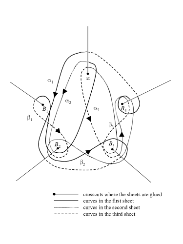
Figure 1. Homology basis $\alpha_{i}$ and $\beta_{i}$, $i=1,2,3$

The half-period matrices for this basis are given by:

$$\omega^{\prime}:=(\omega_{1}^{\prime},\omega_{2}^{\prime},\omega_{3}^{\prime}),\quad\omega^{\prime\prime}:=(\omega_{1}^{\prime\prime},\omega_{2}^{\prime\prime},\omega_{3}^{\prime\prime}),\quad{\Omega}:=\left(\begin{matrix}\omega^{\prime}\\ \omega^{\prime\prime}\end{matrix}\right),$$

where

$$\omega_{a}^{\prime}:=\frac{1}{2}\left[\int_{\alpha_{a}}{\nu^{I}}\right],\quad\omega_{a}^{\prime\prime}:=\frac{1}{2}\left[\int_{\beta_{a}}{\nu^{I}}\right],\quad$$

with the convention that we go around a branchpoint along the paths drawn in Fig. 1, for example we traverse $\beta_{1}$ around $B_{1}$ starting on sheet 1 and crossing over to sheet 3.

A choice of $\alpha$’s and $\beta$’s as in Fig. 1 yields certain relations, which we’ll use in computations even though strictly speaking they hold modulo homotopy. Note that when acting by (powers of) $\zeta_{3}$ we change sheet at a branchpoint: for example, $\displaystyle{\int_{\infty}^{(b_{a},0)}{\nu^{I}}-\hat{\zeta}_{3}\int_{\infty}^{(b_{a},0)}{\nu^{I}}}=\displaystyle{\int_{\infty}^{(b_{a},0)}{\nu^{I}}+\int^{\infty}_{(b_{a},0)}\hat{\zeta}_{3}{\nu^{I}}}$.

Proposition 2.1.

For $\displaystyle{\omega_{a}:=\int_{\infty}^{(b_{a},0)}{\nu^{I}}}$, $(a=1,2,3,4)$ we have following relations:

1. We decompose the $\omega_{a}^{\prime}$ and $\omega_{a}^{\prime\prime}$ in terms of $\hat{\zeta}_{3}^{c}\omega_{a}$,

   $$\omega^{\prime}_{1}=\frac{1}{2}\left((1-\hat{\zeta}_{3}^{2})\omega_{2}+\hat{\zeta}_{3}^{2}(1-\hat{\zeta}_{3}^{2})\omega_{3}+\hat{\zeta}_{3}(1-\hat{\zeta}_{3})\omega_{4}\right),\quad\omega_{a}^{\prime}=\frac{1}{2}\hat{\zeta}_{3}^{a-2}(\hat{\zeta}_{3}-1)\omega_{a},\quad(a=2,3),$$

   $$\omega_{a}^{\prime\prime}=\frac{1}{2}\hat{\zeta}_{3}^{a-2}(\hat{\zeta}_{3}-1)(\omega_{a}-\omega_{a+1}),\quad(a=1,2,3).$$

2. $\hat{\zeta}_{3}^{c}\omega_{a}$ $(c=0,1,a=1,2,3)$, are linear independent over ${\mathbb{Z}}$.

Proof.

(1) is directly obtained from Figure 1. We obtain (2) through the following identities:

(2.2) $$(1+\hat{\zeta}_{3}+\hat{\zeta}_{3}^{2})\omega_{a}=0,$$

$$(1-\hat{\zeta}_{3}^{2})\omega_{1}+\hat{\zeta}_{3}^{2}(1-\hat{\zeta}_{3}^{2})\omega_{2}+\hat{\zeta}_{3}(1-\hat{\zeta}_{3}^{2})\omega_{3}+(1-\hat{\zeta}_{3}^{2})\omega_{4}=0,$$

$$(1-\hat{\zeta}_{3})\omega_{1}+\hat{\zeta}_{3}(1-\hat{\zeta}_{3})\omega_{2}+\hat{\zeta}_{3}^{2}(1-\hat{\zeta}_{3})\omega_{3}+(1-\hat{\zeta}_{3})\omega_{4}=0.$$

The first identity comes from the fact

$$\int_{\infty}^{(x_{1},y_{1})}\begin{pmatrix}{\nu^{I}}_{1}\\ {\nu^{I}}_{2}\\ {\nu^{I}}_{3}\end{pmatrix}+\int_{\infty}^{(x_{1},\zeta_{3}y_{1})}\begin{pmatrix}\zeta_{3}^{2}{\nu^{I}}_{1}\\ \zeta_{3}^{2}{\nu^{I}}_{2}\\ \zeta_{3}{\nu^{I}}_{3}\end{pmatrix}+\int_{\infty}^{(x_{1},\zeta_{3}^{2}y_{1})}\begin{pmatrix}\zeta_{3}{\nu^{I}}_{1}\\ \zeta_{3}{\nu^{I}}_{2}\\ \zeta_{3}^{2}{\nu^{I}}_{3}\end{pmatrix}=0,$$

because $(1+\zeta_{3}+\zeta_{3}^{2})=0$. The others are obtained by integrating along paths which, as seen in Figure 1, are homotopic to a point. ∎

Let $\Lambda$ be the lattice in ${\mathbb{C}}^{3}$ generated by $2\omega^{\prime}$ and $2\omega^{\prime\prime}$. The universal covering space of $X$ is homeomorphic to the space of equivalence classes (up to homotopy) of paths in $X$ which begin at some fixed point $P$; for simplicity, we use the space of paths $\Gamma_{P}X$ because all the functions we define are independent of homotopy. The map $\kappa_{P}:\Gamma_{P}X\to X$ such that for a path $\Gamma_{Q,P}$ from $P$ to $Q$, $\kappa_{P}(\Gamma_{Q,P})=Q$ defines a fiber structure on $\Gamma_{P}X$. The path $\Gamma_{Q,P}$ can be decomposed into $\Gamma_{Q,P}=\sum_{i=1}^{g}(n_{i}\alpha_{i}+n^{\prime}_{i}\beta_{i})+\Gamma^{\prime}_{Q,P}$ up to homology, where $\Gamma^{\prime}_{Q,P}$ is a simple curve from $P$ to $Q$ without any loops in $X$, so that the integral of a holomorphic differential on $\Gamma_{Q,P}$ and $\Gamma^{\prime}_{Q,P}$ is the same, modulo periods.

We extend the Abel map $w$ and define, using the same letter, a map from $\Gamma_{\infty}X$ to ${\mathbb{C}}^{3}$:

$$w(\Gamma_{(x,y),\infty}):=\int_{\Gamma_{(x,y),\infty}}{\nu^{I}},\quad{\nu^{I}}:=\begin{pmatrix}{\nu^{I}}_{1}\\ {\nu^{I}}_{2}\\ {\nu^{I}}_{3}\end{pmatrix}.$$

We simply write $w(x,y)$ for $(x,y)\in X$. We write $(x_{i},y_{i})_{i=1,2,\ldots,k}$ to indicate (by slightly abusing notation) an element of the symmetric product $S^{k}\Gamma_{\infty}X$, and we extend the Abel map by

$$w((x_{i},y_{i})_{i=1,2,\ldots,k})=w(\Gamma_{(x_{i},y_{i}),\infty}|_{i=1,2,\ldots,k}):=\sum_{i=1}^{k}w(\Gamma_{(x_{i},y_{i}),\infty})=\sum_{i=1}^{k}w(x_{i},y_{i}).$$

The map $w$ is surjective for $k\geq 3$ (Abel-Jacobi theorem). We denote by $\mathcal{J}$ the Jacobian of $X$ and by $\kappa$ the natural projection defined by the lattice $\Lambda$,

$$\kappa:{\mathbb{C}}^{3}\to{\mathcal{J}}={\mathbb{C}}^{3}/\Lambda.$$

The strata of ${\mathcal{J}}$, ${\mathcal{W}}_{k}:=\kappa w(S^{k}\Gamma_{\infty}X)$ $(k\geq 1)$, are the same as the sets $\kappa w(S^{k}X)$, abbreviating $w\circ\kappa_{\infty}$ as $w$.

The $\mathbb{Z}_{3}$ action on $X$ induces an action on the Jacobian $\hat{\zeta}_{3}:{\mathcal{J}}\to{\mathcal{J}}$ such that $\hat{\zeta}_{3}^{3}=id$ and equivariantly, a map on a preimage $(P_{1},P_{2},P_{3})\in S^{3}X$ of the Abel map, given by $(\hat{\zeta}_{3}P_{1},\hat{\zeta}_{3}P_{2},\hat{\zeta}_{3}P_{3})$, indeed $\hat{\zeta}_{3}\Lambda=\Lambda$ as seen by the action on the paths of integration.

Proposition 2.2.

$\{3\zeta_{3}^{c}\omega_{a}\}_{a=1,2,3,4,c=0,1,2}$ is a subset of $\Lambda$. For every $3\hat{\zeta}_{3}^{c}\omega_{a}$, there are integers $h^{(c)\prime}_{a,b}$ and $h^{(c)\prime\prime}_{a,b}$ $(a=1,2,3,4,\ b=1,2,3,\ c=0,1,2)$ such that

(2.3) $$\hat{\zeta}_{3}^{c}\omega_{a}=\frac{2}{3}\sum_{b=1}^{3}(h^{(c)\prime}_{a,b}\omega_{b}^{\prime}+h^{(c)\prime\prime}_{a,b}\omega_{b}^{\prime\prime}).$$

Here we point out that even though the values $h^{(c)\prime}_{a,b}$ and $h^{(c)\prime\prime}_{a,b}$ depend upon the choice of the homology basis $\alpha_{a}$ and $\beta_{a}$, the above fact that $3\zeta_{3}^{c}\omega_{a}$ is a point in $\Lambda$ does not, and thus the $\mathrm{al}$-function defined below is invariant under the action of ${\mathrm{Sp}}(6,{\mathbb{Z}})$ on a 3-vector.

Proof.

From $(1-\zeta_{3})(1-\zeta_{3}^{2})=3$, we have

$$\hat{\zeta}_{3}^{2a-1}(\hat{\zeta}_{3}^{2}-1)\omega_{a}^{\prime}=\frac{3}{2}\omega_{a},\quad(a=2,3),\quad\hat{\zeta}_{3}^{2a-2}(\hat{\zeta}_{3}^{2}-1)\omega_{a}^{\prime\prime}=\frac{3}{2}(\omega_{a}-\omega_{a+1}),\quad(a=1,2,3).$$

Then we have the relations: $\omega_{a}=\frac{2}{3}\hat{\zeta}_{3}^{2a-1}(\hat{\zeta}_{3}^{2}-1)\omega_{a}^{\prime}$ $(a=2,3)$, $\omega_{4}=\frac{2}{3}\hat{\zeta}_{3}^{2a-2}(\hat{\zeta}_{3}^{2}-1)(\hat{\zeta}_{3}\omega_{3}^{\prime}-\omega_{3}^{\prime\prime})$, and $\omega_{1}=\frac{2}{3}\hat{\zeta}_{3}^{2a-2}(\hat{\zeta}_{3}^{2}-1)(\omega_{1}^{\prime\prime}+\hat{\zeta}_{3}\omega_{2}^{\prime})$. Since the ${\mathbb{Z}}$-module $\Lambda$ is invariant under the action of $\hat{\zeta}_{3}$, then $2\hat{\zeta}_{3}\omega_{a}^{\prime}\in\Lambda$ and $2\hat{\zeta}_{3}\omega_{a}^{\prime\prime}\in\Lambda$, hence there are integers $p^{(c)\prime}_{a,b}$, $p^{(c)\prime\prime}_{a,b}$, $q^{(c)\prime}_{a,b}$ and $q^{(c)\prime\prime}_{a,b}$, such that

$$\hat{\zeta}_{3}^{c}\omega_{a}^{\prime}=\sum_{b=1}^{3}(p^{(c)\prime}_{a,b}\omega_{b}^{\prime}+p^{(c)\prime\prime}_{a,b}\omega_{b}^{\prime\prime}),\quad\hat{\zeta}_{3}^{c}\omega_{a}^{\prime\prime}=\sum_{b=1}^{3}(q^{(c)\prime}_{a,b}\omega_{b}^{\prime}+q^{(c)\prime\prime}_{a,b}\omega_{b}^{\prime\prime}),$$

which shows the statement. ∎

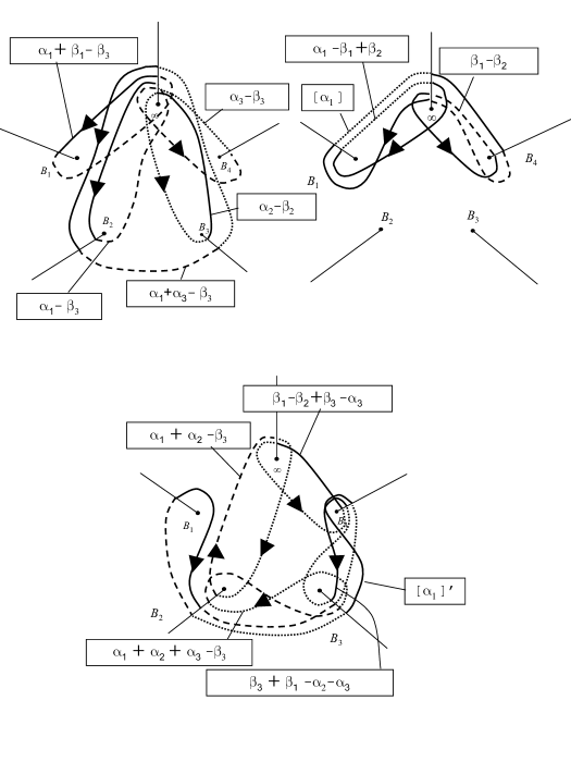
Figure 2. Relations among $\alpha_{i}$ and $\beta_{i}$

Remark 2.3.

We add oriented loops $\gamma$ and $\gamma^{\prime}$ up to equivalence, in the homology group of the curve: $\int_{\gamma+\gamma^{\prime}}{\nu^{I}}=\int_{\gamma}{\nu^{I}}+\int_{\gamma^{\prime}}{\nu^{I}}$. Using the relations in the proof of Proposition 2.1, we can compute the $\omega$’s along the paths in Figure 2, where $[\alpha_{1}]$ is an equivalence class modulo (2.2), though we routinely abuse notation and write simply $\alpha_{1}$. Using Figure 2, one checks identities such as:

$$3\omega_{1}=2\omega_{1}^{\prime}+\omega_{2}^{\prime\prime}-\omega_{3}^{\prime\prime}.$$

Remark 2.4.

We summarize the local behavior of the holomorphic one-forms for use below. In a $t$-series expansion, $d_{\geq}(t^{\ell})$ denotes a term of order greater than or equal to $\ell$.

1. At the point $\infty$, we choose a local parameter $t_{\infty}$ so that $t_{\infty}^{3}=1/x$ and $y={\displaystyle\frac{1}{t_{\infty}^{4}}}(1+d_{\geq}(t_{\infty}))$; the holomorphic one-forms are expanded as,

   $${\nu^{I}}_{1}=-t_{\infty}^{4}(1+d_{\geq}(t_{\infty}))dt_{\infty},\quad{\nu^{I}}_{2}=-t_{\infty}^{3}(1+d_{\geq}(t_{\infty}))dt_{\infty},\quad{\nu^{I}}_{3}=-(1+d_{\geq}(t_{\infty}))dt_{\infty}.$$

2. At $(b_{a},0)$, a local parameter $t_{a}$ is chosen so that $t_{a}^{3}=(x-b_{a})$. Then we have

   $$y=t_{a}C_{a}(1+d_{\geq}(t_{a}^{2})),\quad dx=3t_{a}^{2}dt_{a},$$

   where $C_{a}:=\displaystyle{\left.\sqrt[3]{\frac{df(x)}{dx}}\right|_{x=b_{a}}}$. The holomorphic one-forms are written as,

   $${\nu^{I}}_{1}=\frac{dt_{a}}{C_{a}^{2}}(1+d_{\geq}(t_{a})),\quad{\nu^{I}}_{3}=\frac{t_{a}dt_{a}}{C_{a}}(1+d_{\geq}(t_{a})),\quad{\nu^{I}}_{2}-b_{1}{\nu^{I}}_{1}=\frac{t_{a}^{3}dt_{a}}{C_{a}^{2}}(1+d_{\geq}(t_{a})).$$

   The local chart is a triple covering of the curve projected to the $x$-axis, so there is a natural action $\hat{\iota}^{(a)}_{\zeta_{3}}:t_{a}\to\zeta_{3}t_{a}$. Since $y$ is also a local parameter at a branch point $B_{a}$, locally we can identify the action $\hat{\iota}^{(a)}_{\zeta_{3}}$ with $\hat{\zeta}_{3}$.

The following meromorphic functions $\{\phi_{i}\}$ on $X$ belong to the ring $R:={\mathbb{C}}[x,y]/(y^{3}-\prod(x-b_{r}))$,

(2.4) $$\phi_{i}=\left\{\begin{matrix}x&\mbox{for }i=3\\ y&\mbox{for }i=4\\ x^{(i-3)/3+2}&\mbox{for }i>3,i\equiv 0\mbox{ modulo }3,\\ x^{(i-3)/3+1}y&\mbox{for }i>3,i\equiv 1\mbox{ modulo }3,\\ x^{(i-3)/3}y^{2}&\mbox{for }i>3,i\equiv 2\mbox{ modulo }3.\end{matrix}\right.$$

In particular, $\phi_{n}$ has a pole of order $N(n)$ at $\infty$, with:

(2.5) $$N(0)=0,\quad N(1)=3,\quad N(2)=4,\quad N(3)=6,\quad N(n)=n+3,\quad\mbox{for }n>3.$$

Lastly, we identify the Jacobian with $\mathrm{Pic}^{0}(X)$ by choosing $\infty$ as the base point, so we embed $X$ in $\mathcal{J}$ by sending a point $P\in X$ to the sheaf associated to the divisor $P-\infty$ (up to linear equivalence).

3. Addition law. I

The additive inverse in ${\mathbb{C}}^{3}$ and ${\mathcal{J}}$ corresponds to a bijection from $S^{3}X$ to itself, which depends on our choice of base point. We note that in the hyperelliptic case this corresponds simply to the hyperelliptic involution $(x,y)\to(x,-y)$, in the (cyclic) trigonal case we need a modification as in [MP, Lemma 2.6].

We now give an explicit realization of the Serre involution on $\mathrm{Pic}^{(g-1)}$:

$$\mathcal{L}\to K_{X}\mathcal{L}^{-1},$$

which will be used in the development below.

The following proposition [MP, Lemma 2.6] holds:

Proposition 3.1.

For a positive integer $n$, there is a natural inclusion satisfying

$$[-1]:{\mathcal{W}}_{n}\to{\mathcal{W}}_{N(n)-n},\quad(u\mapsto-u).$$

We construct an algorithm to give the $[-1]$-action explicitly in order to define the trigonal $\mathrm{al}$ function.

Definition 3.2.

For $(P,(P_{1},\cdots,P_{n}))$ $\in(X-\infty)\times S^{n}(X-\infty)$, we define $\mu_{n}(P)$ by

$$\mu_{n}(P):=\mu_{n}(P;P_{1},\ldots,P_{n}):=\lim_{P_{i}^{\prime}\to P_{i}}{\displaystyle\frac{\left|\begin{matrix}1&\phi_{1}(P_{1}^{\prime})&\cdots&\phi_{n}(P_{1}^{\prime})\\ 1&\phi_{1}(P_{2}^{\prime})&\cdots&\phi_{n}(P_{2}^{\prime})\\ \vdots&\vdots&\ddots&\vdots\\ 1&\phi_{1}(P_{n}^{\prime})&\cdots&\phi_{n}(P_{n}^{\prime})\\ 1&\phi_{1}(P)&\cdots&\phi_{n}(P)\end{matrix}\right|}{\left|\begin{matrix}1&\phi_{1}(P_{1}^{\prime})&\cdots&\phi_{n-1}(P_{1}^{\prime})\\ 1&\phi_{1}(P_{2}^{\prime})&\cdots&\phi_{n-1}(P_{2}^{\prime})\\ \vdots&\vdots&\ddots&\vdots\\ 1&\phi_{1}(P_{n}^{\prime})&\cdots&\phi_{n-1}(P_{n}^{\prime})\end{matrix}\right|}},$$

and since the $\phi$’s are algebraic functions on $X$, we extend the domain to $X\times S^{n}(X)$, allowing for poles.

More details on this function are given in [MP], where it is shown that it can be viewed as a generalization of the $F$ in (1.1) or $U$ in the triple of polynomials that Mumford calls $(U,V,W)$ in the hyperelliptic case [Mum, Ch. IIIa].

In the following Lemma, we show that $\mu_{n}(P)$ is associated with the addition structure on the divisor group of $X$ from a classical viewpoint. Let $S^{n}_{1}(X)$ be defined as

$$\Bigr{\{}(P_{1},\ldots,P_{n})\in S^{n}(X)\ |\ \exists\{{i_{1}},\ldots,{i_{k}}\}\subset\{1,\ldots,n\}\mbox{ such that }\mu_{k}(P_{i_{1}},\ldots,P_{i_{k}})=0\Bigr{\}}.$$

For $(P_{i})_{i=1,\ldots,n}\in S^{n}(X-\infty)\setminus S^{n}_{1}(X-\infty)$, $\mu_{n}(P;P_{1},\ldots,P_{n})$ has the following properties:

1. It is monic,

2. At each $P=P_{i}$, it has a simple zero,

3. $\mu_{n}(P)$ has a pole at $\infty$ of order $N(n)$, and

4. $\mu_{n}(P)$ has $(N(n)-n)$ zeros aside from the $P_{i}$’s $(i=1,\ldots,n)$.

Lemma 3.3.

Let $n$ be a positive integer. For $(P_{i})_{i=1,\ldots,n}\in S^{n}(X-\infty)$, $\mu_{n}$ is consistent with the following diagram, where $[-1]_{n}$: $S^{n}(X-\infty)\to S^{N(n)-n}(X)$ such that

$$\begin{CD}S^{n}(X-\infty)@>{[-1]_{n}}>{}>S^{N(n)-n}(X)\\ @V{w}V{}V@V{w}V{}V\\ {\mathcal{W}}_{n}@>{[-1]}>{}>{\mathcal{W}}_{N(n)-n}\\ \end{CD},$$

i.e., $(P_{i})_{i=1,\ldots,n}\in S^{n}(X-\infty)$ corresponds to an element $(Q_{i})_{i=1,\ldots,N(n)-n}\in S^{N(n)-n}(X)$, such that

$$\sum_{i=1}^{n}P_{i}-n\infty\sim-\sum_{i=1}^{N(n)-n}Q_{i}+(N(n)-n)\infty.$$

4. Addition law: examples

In this section, we compute $[-1]_{n}$ $(n=1,2,3)$ explicitly, based on Lemma 3.3, to demonstrate the significance of $\mu_{n}$.

4.1. $[-1]_{1}P$:

To find $[-1]_{1}(x_{1},y_{1})$, recall that N(1)=3, so we seek a divisor of degree two. For the divisor of a meromorphic function of $(x,y)$,

$$\left|\begin{matrix}1&x_{1}\\ 1&x\\ \end{matrix}\right|=0$$

implies that $x=x_{1}.$ This means that

$$(x_{1},y_{1})+(x_{1},\zeta_{3}y_{1})+(x_{1},\zeta_{3}^{2}y_{1})-3\infty\sim 0.$$

In other words, as sheaves,

(4.1) $$[-1]_{1}(x_{1},y_{1})=(x_{1},\zeta_{3}y_{1})+(x_{1},\zeta_{3}^{2}y_{1}).$$

This means

$$\int_{\infty}^{(x_{1},y_{1})}\begin{pmatrix}{\nu^{I}}_{1}\\ {\nu^{I}}_{2}\\ {\nu^{I}}_{3}\end{pmatrix}+\int_{\infty}^{(x_{1},\zeta_{3}y_{1})}\begin{pmatrix}\zeta_{3}^{2}{\nu^{I}}_{1}\\ \zeta_{3}^{2}{\nu^{I}}_{2}\\ \zeta_{3}{\nu^{I}}_{3}\end{pmatrix}+\int_{\infty}^{(x_{1},\zeta_{3}^{2}y_{1})}\begin{pmatrix}\zeta_{3}{\nu^{I}}_{1}\\ \zeta_{3}{\nu^{I}}_{2}\\ \zeta_{3}^{2}{\nu^{I}}_{3}\end{pmatrix}\equiv 0,\quad\mbox{modulo }\Lambda.$$

4.2. $[-1]_{2}(P_{1}+P_{2})$:

Let $Q_{a}=(x^{\prime}_{a},y^{\prime}_{a})$ ($a=1,2$) be a solution of $\mu_{3}(P,P_{1},P_{2})$ different from $P_{a}$, i.e.,

$$w(Q_{1}+Q_{2})=-w(P_{1}+P_{2}),\quad{i.e.},(Q_{1},Q_{2})=[-1]_{2}(P_{1},P_{2}).$$

Since

(4.2) $$\left|\begin{matrix}1&x_{1}&y_{1}\\ 1&x_{2}&y_{2}\\ 1&x_{a}^{\prime}&y_{a}^{\prime}\\ \end{matrix}\right|=\left|\begin{matrix}x_{1}&y_{1}\\ x_{2}&y_{2}\\ \end{matrix}\right|-\left|\begin{matrix}1&y_{1}\\ 1&y_{2}\\ \end{matrix}\right|x_{a}^{\prime}+\left|\begin{matrix}1&x_{1}\\ 1&x_{2}\\ \end{matrix}\right|y_{a}^{\prime}=0,$$

then direct computations provide the following lemma:

Lemma 4.1.

For the points obeying (4.2) the following relations hold:

$$\begin{split}&\left|\begin{matrix}x_{1}&y_{1}\\ x_{2}&y_{2}\\ \end{matrix}\right|\left|\begin{matrix}1&y_{1}^{\prime}\\ 1&y_{2}^{\prime}\\ \end{matrix}\right|=\left|\begin{matrix}x_{1}^{\prime}&y_{1}^{\prime}\\ x_{2}^{\prime}&y_{2}^{\prime}\\ \end{matrix}\right|\left|\begin{matrix}1&y_{1}\\ 1&y_{2}\\ \end{matrix}\right|,\quad\left|\begin{matrix}x_{1}&y_{1}\\ x_{2}&y_{2}\\ \end{matrix}\right|\left|\begin{matrix}1&x_{1}^{\prime}\\ 1&x_{2}^{\prime}\\ \end{matrix}\right|=\left|\begin{matrix}x_{1}^{\prime}&y_{1}^{\prime}\\ x_{2}^{\prime}&y_{2}^{\prime}\\ \end{matrix}\right|\left|\begin{matrix}1&x_{1}\\ 1&x_{2}\\ \end{matrix}\right|,\\ &\left|\begin{matrix}1&y_{1}\\ 1&y_{2}\\ \end{matrix}\right|\left|\begin{matrix}1&x_{1}^{\prime}\\ 1&x_{2}^{\prime}\\ \end{matrix}\right|=\left|\begin{matrix}1&y_{1}^{\prime}\\ 1&y_{2}^{\prime}\\ \end{matrix}\right|\left|\begin{matrix}1&x_{1}\\ 1&x_{2}\\ \end{matrix}\right|.\end{split}$$

This shows that if $P_{1}$ and $P_{2}$ are generic in the sense that none of the determinants in Lemma 4.1 vanishes, then $Q_{1}$ and $Q_{2}$ have the same property.

4.3. $[-1]_{3}(P_{1}+P_{2}+P_{3})$

Let

$$(Q_{1},Q_{2},Q_{3})=[-1]_{3}(P_{1},P_{2},P_{3}).$$

In other words $Q_{a}=(x^{\prime}_{a},y^{\prime}_{a})$ ($a=1,2,3$) are solutions of $\mu_{3}(P,P_{1},P_{2},P_{3})$ which differ from $P_{b}$ ($b=1,2,3$).

(4.3) $$\left|\begin{matrix}1&x_{1}&y_{1}&x_{1}^{2}\\ 1&x_{2}&y_{2}&x_{2}^{2}\\ 1&x_{3}&y_{3}&x_{3}^{2}\\ 1&x^{\prime}_{a}&y^{\prime}_{a}&{x^{\prime}}_{a}^{2}\\ \end{matrix}\right|=0.$$

Similar to Lemma 4.1, we have the following result:

Lemma 4.2.

For $\{i_{1},i_{2},i_{3}\},\{j_{1},j_{2},j_{3}\}\subset\{0,1,2,3\}$, the following relation holds

$$\begin{split}&\left|\begin{matrix}\phi_{i_{1}}(P_{1})&\phi_{i_{2}}(P_{1})&\phi_{i_{3}}(P_{1})\\ \phi_{i_{1}}(P_{2})&\phi_{i_{2}}(P_{2})&\phi_{i_{3}}(P_{2})\\ \phi_{i_{1}}(P_{3})&\phi_{i_{2}}(P_{3})&\phi_{i_{3}}(P_{3})\\ \end{matrix}\right|\left|\begin{matrix}\phi_{j_{1}}(Q_{1})&\phi_{j_{2}}(Q_{1})&\phi_{j_{3}}(Q_{1})\\ \phi_{j_{1}}(Q_{2})&\phi_{j_{2}}(Q_{2})&\phi_{j_{3}}(Q_{2})\\ \phi_{j_{1}}(Q_{3})&\phi_{j_{2}}(Q_{3})&\phi_{j_{3}}(Q_{3})\\ \end{matrix}\right|\\ =&\epsilon_{i_{1},i_{2},i_{3},j_{1},j_{2},j_{3}}\left|\begin{matrix}\phi_{j_{1}}(P_{1})&\phi_{j_{2}}(P_{1})&\phi_{j_{3}}(P_{1})\\ \phi_{j_{1}}(P_{2})&\phi_{j_{2}}(P_{2})&\phi_{j_{3}}(P_{2})\\ \phi_{j_{1}}(P_{3})&\phi_{j_{2}}(P_{3})&\phi_{j_{3}}(P_{3})\\ \end{matrix}\right|\left|\begin{matrix}\phi_{i_{1}}(Q_{1})&\phi_{i_{2}}(Q_{1})&\phi_{i_{3}}(Q_{1})\\ \phi_{i_{1}}(Q_{2})&\phi_{i_{2}}(Q_{2})&\phi_{i_{3}}(Q_{2})\\ \phi_{i_{1}}(Q_{3})&\phi_{i_{2}}(Q_{3})&\phi_{i_{3}}(Q_{3})\\ \end{matrix}\right|,\end{split}$$

where $\epsilon_{i_{1},i_{2},i_{3},j_{1},j_{2},j_{3}}$ is an appropriate sign.

5. Functions $A_{r}$ and $F_{r}$

In order to construct the trigonal $\mathrm{al}_{r}$ function of the curve $X$, we introduce meromorphic functions $A_{r}$ and $F_{r}$.

On a hyperelliptic curve, as shown in (1.1), the $\mathrm{al}$ function is alternatively defined by $\mathrm{al}_{r}(u):=\sqrt{F(b_{r})}$ up to a constant factor, where $(x,y)=(b_{r},0)=B_{r}$ is a branch point of the curve.

In order to define the trigonal version of $\mathrm{al}$ function, we also deal with the value of the function $\mu$ in (5.1) at a branch point $B_{r}$.

Definition 5.1.

For a branch point $B_{a}$ of $X$ and $P_{i}=(x_{i},y_{i})$ $(i=1,2,3)$ determining a point of $S^{3}X$, we define the meromorphic functions:

(5.1) $$\begin{split}A_{a}(P_{1},P_{2},P_{3})&:=\mu(B_{a};P_{1},P_{2},P_{3})=\displaystyle{\frac{\left|\begin{matrix}1&x_{1}&y_{1}&{x_{1}}^{2}\\ 1&x_{2}&y_{2}&{x_{2}}^{2}\\ 1&x_{3}&y_{3}&{x_{3}}^{2}\\ 1&b_{a}&0&b_{a}^{2}\\ \end{matrix}\right|}{\left|\begin{matrix}1&x_{1}&y_{1}\\ 1&x_{2}&y_{2}\\ 1&x_{3}&y_{3}\\ \end{matrix}\right|}},\\ F_{a}(P_{1},P_{2},P_{3})&:=(b_{a}-x_{1})(b_{a}-x_{2})(b_{a}-x_{3}).\\ \end{split}$$

Let $\deg_{P}h$ denote the order of zero or pole of a meromorphic function $h$ at $P$.

Proposition 5.2.

$A_{a}$ and $F_{a}$ have the following zeros and poles:

1. For generic points $P_{1},P_{2}$ of $X$,

   $$\deg_{(B_{a},P_{1},P_{2})}A_{a}(P_{1},P_{2},P_{3})=1,\quad\deg_{(B_{a},P_{1},P_{2})}F_{a}(P_{1},P_{2},P_{3})=3.\quad$$

2. For generic points $P_{1},P_{2}$ of $X$,

   $$\deg_{[-1]_{3}([-1]_{2}(P_{1},P_{2}),B_{a})}A_{a}=1,\quad\deg_{[-1]_{3}([-1]_{2}(P_{1},P_{2}),B_{a})}F_{a}=0.\quad$$

3. For generic points $P_{1},P_{2}$ of $X$,

   $$\deg_{(\infty,P_{1},P_{2})}A_{a}=-2,\quad\deg_{(\infty,P_{1},P_{2})}F_{a}=-3.\quad$$

4. For generic points $P_{1}$ of $X$,

   $$\deg_{([-1](b_{a},0),P_{1})}A_{a}=3,\quad\deg_{([-1](b_{a},0),P_{1})}F_{a}=6.\quad$$

Proof.

(1) follows from the definition. (3) is obvious because for $P_{3}$ near $\infty$, we have

(5.2) $$\begin{split}A_{a}(P_{1},P_{2},P_{3})&=\frac{\left|\begin{matrix}1&x_{2}&y_{2}\\ 1&x_{3}&y_{3}\\ 1&b_{2}&0\\ \end{matrix}\right|x_{1}^{2}}{\left|\begin{matrix}1&x_{2}\\ 1&x_{3}\\ \end{matrix}\right|y_{1}}(1+d_{\geq}(t_{\infty}^{2}))=\frac{\left|\begin{matrix}1&x_{2}&y_{2}\\ 1&x_{3}&y_{3}\\ 1&b_{2}&0\\ \end{matrix}\right|}{\left|\begin{matrix}1&x_{2}\\ 1&x_{3}\\ \end{matrix}\right|}\frac{1}{t_{\infty}^{2}}(1+d_{\geq}(t_{\infty}^{2})),\\ F_{a}(P_{1},P_{2},P_{3})&=\frac{1}{t_{\infty}^{3}}+d_{\geq}(t_{\infty}^{2}).\quad\end{split}$$

To prove (2), we denote by $C_{a}:=\left.{\displaystyle\frac{dy}{dt_{a}}}\right|_{x=b_{a}}$, we assume that $P_{1}$ and $P_{2}$ are generic points and $P_{3}$ is close to $B_{a}$; $P_{3}=(x_{3},y_{3})$ behaves like $(b_{a}+t_{a}^{3}+d_{\geq}(t_{a}^{4}),\zeta_{3}^{i}C_{a}t_{a}+d_{\geq}(t_{a}^{2}))$. Let

$$(Q_{1},Q_{2})=[-1]_{2}(P_{1},P_{2}),\quad(Q_{1}^{\prime},Q_{2}^{\prime},Q_{3}^{\prime})=[-1]_{3}(Q_{1},Q_{2},P_{3}),$$

where $Q_{a}=(x^{\prime}_{a},y^{\prime}_{a})$ and $Q^{\prime}_{a}=(x^{\prime\prime}_{a},y^{\prime\prime}_{a})$, i.e.,

$$\left|\begin{matrix}1&x_{1}&{y_{1}}\\ 1&x_{2}&{y_{2}}\\ 1&x_{c}^{\prime}&{y_{c}^{\prime}}\\ \end{matrix}\right|=0,\quad\left|\begin{matrix}1&x_{1}^{\prime}&{y_{1}^{\prime}}&{x_{1}^{\prime}}^{2}\\ 1&x_{2}^{\prime}&{y_{2}^{\prime}}&{x_{2}^{\prime}}^{2}\\ 1&x_{3}&{y_{3}}&{x_{3}}^{2}\\ 1&x_{c}^{\prime\prime}&{y_{c}^{\prime\prime}}&{x_{c}^{\prime\prime}}^{2}\\ \end{matrix}\right|=0.$$

We consider the expansion of $A_{a}$ and $F_{a}$. First we look at $F_{a}$. When $P_{3}$ is equal to $B_{a}$, $F_{a}$ becomes

(5.3) $$\left|\begin{matrix}1&x_{1}^{\prime\prime}&{x_{1}^{\prime\prime}}^{2}&{x_{1}^{\prime\prime}}^{3}\\ 1&x_{2}^{\prime\prime}&{x_{2}^{\prime\prime}}^{2}&{x_{2}^{\prime\prime}}^{3}\\ 1&x_{3}^{\prime\prime}&{x_{3}^{\prime\prime}}^{2}&{x_{3}^{\prime\prime}}^{3}\\ 1&b_{a}&b_{a}^{2}&b_{a}^{3}\\ \end{matrix}\right|\Bigr{/}\left|\begin{matrix}1&x_{1}^{\prime\prime}&{x_{1}^{\prime\prime}}^{2}\\ 1&x_{2}^{\prime\prime}&{x_{2}^{\prime\prime}}^{2}\\ 1&x_{3}^{\prime\prime}&{x_{3}^{\prime\prime}}^{2}\\ \end{matrix}\right|,$$

and if it vanished then one of the $Q^{\prime}$’s would equal $(b_{a}+t^{3},\zeta_{3}C_{a}t)$ near $t=0$ but $(b_{a}+t^{3},\zeta_{3}C_{a}t)$ does not satisfy (4.2).

We now compute $A_{a}$ as follows:

$$\begin{split}A_{a}(Q^{\prime}_{1},Q^{\prime}_{2},Q^{\prime}_{3})&=\displaystyle{\frac{\left|\begin{matrix}1&x_{1}^{\prime\prime}&y_{1}^{\prime\prime}&{x_{1}^{\prime\prime}}^{2}\\ 1&x_{2}^{\prime\prime}&y_{2}^{\prime\prime}&{x_{2}^{\prime\prime}}^{2}\\ 1&x_{3}^{\prime\prime}&y_{3}^{\prime\prime}&{x_{3}^{\prime\prime}}^{2}\\ 1&b_{a}&0&b_{a}^{2}\\ \end{matrix}\right|}{\left|\begin{matrix}1&x_{1}^{\prime\prime}&y_{1}^{\prime\prime}\\ 1&x_{2}^{\prime\prime}&y_{2}^{\prime\prime}\\ 1&x_{3}^{\prime\prime}&y_{3}^{\prime\prime}\\ \end{matrix}\right|}}.\\ \end{split}$$

Direct computation gives the numerator as:

(5.4) $$\left|\begin{matrix}x_{1}^{\prime\prime}&y_{1}^{\prime\prime}&{x_{1}^{\prime\prime}}^{2}\\ x_{2}^{\prime\prime}&y_{2}^{\prime\prime}&{x_{2}^{\prime\prime}}^{2}\\ x_{3}^{\prime\prime}&y_{3}^{\prime\prime}&{x_{3}^{\prime\prime}}^{2}\\ \end{matrix}\right|-\left|\begin{matrix}1&y_{1}^{\prime\prime}&{x_{1}^{\prime\prime}}^{2}\\ 1&y_{2}^{\prime\prime}&{x_{2}^{\prime\prime}}^{2}\\ 1&y_{3}^{\prime\prime}&{x_{3}^{\prime\prime}}^{2}\\ \end{matrix}\right|b_{a}-\left|\begin{matrix}1&x_{1}^{\prime\prime}&y_{1}^{\prime\prime}\\ 1&x_{2}^{\prime\prime}&y_{2}^{\prime\prime}\\ 1&x_{3}^{\prime\prime}&y_{3}^{\prime\prime}\\ \end{matrix}\right|b_{a}^{2}.$$

Due to the relations in Lemma 4.2, this equals

(5.5) $$\frac{\left|\begin{matrix}1&x_{1}^{\prime\prime}&{x_{1}^{\prime\prime}}^{2}\\ 1&x_{2}^{\prime\prime}&{x_{2}^{\prime\prime}}^{2}\\ 1&x_{3}^{\prime\prime}&{x_{3}^{\prime\prime}}^{2}\\ \end{matrix}\right|}{\left|\begin{matrix}1&x_{1}^{\prime}&{x_{1}^{\prime}}^{2}\\ 1&x_{2}^{\prime}&{x_{2}^{\prime}}^{2}\\ 1&b_{a}&{b_{a}}^{2}\\ \end{matrix}\right|}\times\left|\begin{matrix}1&x_{1}^{\prime}&y_{1}^{\prime}&{x_{1}^{\prime}}^{2}\\ 1&x_{2}^{\prime}&y_{2}^{\prime}&{x_{2}^{\prime}}^{2}\\ 1&x_{3}^{\prime}&y_{3}^{\prime}&{x_{3}^{\prime}}^{2}\\ 1&b_{a}&0&b_{a}^{2}\\ \end{matrix}\right|=\frac{\left|\begin{matrix}1&x_{1}^{\prime\prime}&{x_{1}^{\prime\prime}}^{2}\\ 1&x_{2}^{\prime\prime}&{x_{2}^{\prime\prime}}^{2}\\ 1&x_{3}^{\prime\prime}&{x_{3}^{\prime\prime}}^{2}\\ \end{matrix}\right|}{\left|\begin{matrix}1&x_{1}^{\prime}&{x_{1}^{\prime}}^{2}\\ 1&x_{2}^{\prime}&{x_{2}^{\prime}}^{2}\\ 1&b_{a}&{b_{a}}^{2}\\ \end{matrix}\right|}\times\left(\left|\begin{matrix}1&x_{1}^{\prime}&y_{1}^{\prime}&{x_{1}^{\prime}}^{2}\\ 1&x_{2}^{\prime}&y_{2}^{\prime}&{x_{2}^{\prime}}^{2}\\ 1&b_{a}&C_{a}t_{a}&b_{a}^{2}\\ 1&b_{a}&0&b_{a}^{2}\\ \end{matrix}\right|+d_{\geq}(t_{a}^{2})\right).$$

We consider the factors in this formula. The fact that $Q_{1}$ and $Q_{2}$ are generic for generic $P_{1}$ and $P_{2}$, and (4.3) imply that both

$$\left|\begin{matrix}1&x_{1}^{\prime\prime}&{x_{1}^{\prime\prime}}^{2}\\ 1&x_{2}^{\prime\prime}&{x_{2}^{\prime\prime}}^{2}\\ 1&x_{3}^{\prime\prime}&{x_{3}^{\prime\prime}}^{2}\\ \end{matrix}\right|\quad\mbox{and}\quad\left|\begin{matrix}1&x_{1}^{\prime}&{x_{1}^{\prime}}^{2}\\ 1&x_{2}^{\prime}&{x_{2}^{\prime}}^{2}\\ 1&b_{a}&{b_{a}}^{2}\\ \end{matrix}\right|$$

do not vanish in the limit $P_{3}\to B_{a}$. Hence $A_{a}$ has a simple zero at $B_{a}$.

To prove (4), we consider $P_{1}$ and $P_{2}$ near $B_{a}$; $P_{i}=(x_{i},y_{i})$ behaves like $(t_{b}^{3}+b_{a},\zeta_{3}^{i}C_{a}t_{b}+d_{\geq}(t_{b}^{2}))$, $i=1,2$. Let us consider the behavior of $A_{a}$ and $F_{a}$.

$$\begin{split}A_{a}(P_{1},P_{2},P_{3})&=\displaystyle{\frac{\left|\begin{matrix}1&b_{a}+t_{a}^{3}+d_{\geq}(t_{a}^{4})&\zeta_{3}C_{a}t_{a}+d_{\geq}(t_{a}^{3})&(b_{a}+t_{a}^{3})^{2}+d_{\geq}(t_{a}^{4})\\ 1&b_{a}+t_{a}^{3}+d_{\geq}(t_{a}^{4})&\zeta_{3}^{2}C_{a}t_{a}+d_{\geq}(t_{a}^{3})&(b_{a}+t_{a}^{3})^{2}+d_{\geq}(t_{a}^{4})\\ 1&x_{3}&y_{3}&x_{3}^{2}\\ 1&b_{a}&0&b_{a}^{2}\\ \end{matrix}\right|}{\left|\begin{matrix}1&b_{a}+t_{a}^{3}+d_{\geq}(t_{a}^{4})&\zeta_{3}C_{a}t_{a}+d_{\geq}(t_{a}^{2})\\ 1&b_{a}+t_{a}^{3}+d_{\geq}(t_{a}^{4})&\zeta_{3}^{2}C_{a}t_{a}+d_{\geq}(t_{a}^{2})\\ 1&x_{3}&y_{3}\\ \end{matrix}\right|}}\\ \end{split}$$

$$\begin{split}&=\displaystyle{\frac{\left|\begin{matrix}0&0&(\zeta_{3}-\zeta_{3}^{2})C_{a}+d_{\geq}(t_{a}^{3})&0\\ 1&b_{a}+t_{a}^{3}+d_{\geq}(t_{a}^{4})&\zeta_{3}^{2}C_{a}t_{a}+d_{\geq}(t_{a}^{3})&(b_{a}+t_{a}^{3})^{2}+d_{\geq}(t_{a}^{4})\\ 1&x_{3}&y_{3}&x_{3}^{2}\\ 1&b_{a}&0&b_{a}^{2}\\ \end{matrix}\right|}{\left|\begin{matrix}1&b_{a}+t_{a}^{3}+d_{\geq}(t_{a}^{4})&\zeta_{3}C_{a}t_{a}+d_{\geq}(t_{a}^{2})\\ 0&0&(\zeta_{3}^{2}-\zeta_{3})C_{a}t_{a}+d_{\geq}(t_{a}^{2})\\ 1&x_{3}&y_{3}\\ \end{matrix}\right|}}.\\ \end{split}$$

Direct computation shows that this equals $t_{a}^{3}(b_{a}-x_{3})$, and in turn $F_{a}(P_{1},P_{2},P_{3})=t_{a}^{6}(b_{a}-x_{3})$. ∎

We note that (1) and (3) in Proposition 5.2 give the multiplicity of zeros and poles of $F_{a}$ when viewed as a function over $X\times S^{2}X$. In particular, $F_{a}$ does not vanish at $[-1]_{3}([-1]_{2}(P_{1},P_{2}),B_{a})$.

6. The sigma function

We introduce the $\sigma$ function corresponding to $X$, an entire function over $\kappa^{-1}({\mathcal{J}})$, following [EEMÔP1, EEMÔP2, Section 3]. We recall the definition of $\sigma$ and its properties without proofs.

We introduce the period matrices by

(6.1) $$\left[\,\eta^{\prime}\ \eta^{\prime\prime}\right]=\frac{1}{2}\left[\int_{\alpha_{i}}{\nu^{II}}_{j}\ \ \int_{\beta_{i}}{\nu^{II}}_{j}\right]_{i,j=1,2,3},$$

where ${\nu^{II}}_{j}$’s are the differentials of the second kind [EEMÔP2, (1.21) and (1.22)],

$${\nu^{II}}_{1}(x,y)=\frac{x^{2}}{3y^{2}}dx,\quad{\nu^{II}}_{1}(x,y)=\frac{2xy}{3y^{2}}dx,\quad{\nu^{II}}_{1}(x,y)=\frac{(5x^{2}+3\lambda_{3}x+\lambda_{2})y}{3y^{2}}dx.$$

Proposition 6.1.

The matrix,

(6.2) $$M:=\left[\begin{array}[]{cc}2\omega^{\prime}&2\omega^{\prime\prime}\\ 2\eta^{\prime}&2\eta^{\prime\prime}\end{array}\right],$$

satisfies

(6.3) $$M\left[\begin{array}[]{cc}&-1\\ 1&\end{array}\right]{}^{t}{M}=2\pi\sqrt{-1}\left[\begin{array}[]{cc}&-1\\ 1&\end{array}\right].$$

This provides a symplectic structure in the Jacobian which is known as generalized Legendre relation [Ba1, BEL2]. It is known that ${\omega^{\prime}}^{-1}\omega^{\prime\prime}$ is a symmetric, positive-definite matrix.

As shown by Riemann [F], $\text{Im}\,({\omega^{\prime}}^{-1}\omega^{\prime\prime})$ is positive definite. Noting Theorem 1.1 in [F], let

(6.4) $$\delta:=\left[\begin{array}[]{cc}\delta^{\prime\prime}\\ \delta^{\prime}\end{array}\right]\in\left(\tfrac{1}{2}{\mathbb{Z}}\right)^{6}$$

be the theta characteristic which gives the Riemann constant with respect to the base point $\infty$ and the period matrix $[\,\omega^{\prime}\ \omega^{\prime\prime}]$.

For $u\in\mathbb{C}^{g}$, we define

$$\sigma(u) = \sigma(u;M)=\sigma(u_{1},u_{2},u_{3};M)$$

$$= c\,\text{exp}(-\tfrac{1}{2}u\eta^{\prime}{\omega^{\prime}}^{-1}\ {}^{t}\negthinspace u)\vartheta\negthinspace\left[\delta\right](\frac{1}{2}{\omega^{\prime}}^{-1}\ {}^{t}\negthinspace u;\ {\omega^{\prime}}^{-1}\omega^{\prime\prime})$$

$$= c\,\text{exp}(-\tfrac{1}{2}u\eta^{\prime}{\omega^{\prime}}^{-1}\ {}^{t}\negthinspace u)$$

$$\times \sum_{n\in{\mathbb{Z}}^{3}}\exp\big{[}\pi{\sqrt{-1}}\big{\{}\ ^{t}\negthinspace(n+\delta^{\prime\prime}){\omega^{\prime}}^{-1}\omega^{\prime\prime}(n+\delta^{\prime\prime})+\ ^{t}\negthinspace(n+\delta^{\prime\prime})({\omega^{\prime}}^{-1}\,u+\delta^{\prime})\big{\}}\big{]},$$

where $c$ is a certain constant. In this article, the constant $c$ is chosen in such a way that the local expansion of $\sigma$ is consistent with Proposition 6.2 (2).

For a given $u\in{\mathbb{C}}^{3}$, we introduce the notation $u^{\prime}$ and $u^{\prime\prime}$ for the ${\mathbb{R}}^{3}$-vectors such that

$$u=2\omega^{\prime}u^{\prime}+2\omega^{\prime\prime}u^{\prime\prime}.$$

A ‘shifted theta divisor’ $\Theta_{2}$ is the vanishing locus of $\sigma$;

(6.6) $$\Theta_{2}={\mathcal{W}}_{2}\cup[-1]{\mathcal{W}}_{2}={\mathcal{W}}_{2}.$$

Here we summarize the properties of $\sigma(u;M)$ as follows:

Proposition 6.2.

For all $u\in{\mathbb{C}}^{3}$, $\ell\in\Lambda$, and $\gamma\in\mathrm{Sp}(6,{{\mathbb{Z}}})$, we have :

1. $$\sigma(u;\gamma M)=\sigma(u;M).$$

2. $u\mapsto\sigma(u;M)$ has zeroes of order $1$ along $\Theta_{2}={\mathcal{W}}_{2}$;

   $$\sigma(u;M)=0\iff u\in\Theta_{2}.$$

   $\sigma$ has the following expansion near $\Theta_{2}$,

   $$\sigma(u)=(u_{1}-u_{3}u_{2}^{2}+\frac{1}{20}u_{3}^{5})+\mbox{higher-weight terms}.$$

3. For $u$, $v\in{\mathbb{C}}^{3}$, and $\ell$ ($=2\omega^{\prime}\ell^{\prime}+2\omega^{\prime\prime}\ell^{\prime\prime}$) $\in\Lambda$, we define

   $$L(u,v) :=2{}^{t}{u}(\eta^{\prime}v^{\prime}+\eta^{\prime\prime}v^{\prime\prime}),$$

   $$\chi(\ell) :=\exp[\pi\sqrt{-1}\big{(}2({}^{t}{\ell^{\prime}}\delta^{\prime\prime}-{}^{t}{\ell^{\prime\prime}}\delta^{\prime})+{}^{t}{\ell^{\prime}}\ell^{\prime\prime}\big{)}]\ (\in\{1,\,-1\}).$$

   The following holds

   $$\sigma(u+\ell)=\sigma(u)\exp(L(u+\frac{1}{2}\ell,\ell))\chi(\ell).$$

4. For the action $\hat{\zeta}_{3}$ on $u$ defined in Section 2, we have

   $$\sigma(\hat{\zeta}_{3}u)=\zeta_{3}\sigma(u),\quad\hat{\zeta}_{3}\Theta_{2}=\Theta_{2}.$$

Proof.

See [EEMÔP2]. ∎

Proposition 6.3.

For $\ell\in\Lambda$ as in Proposition 6.2,

(6.7) $$\sigma(u+\hat{\zeta}_{3}\ell)=\sigma(u)\exp(L(\hat{\zeta}_{3}^{2}u+\frac{1}{2}\ell,\ell))\chi(\ell).$$

Proof.

By considering $\sigma(\hat{\zeta}_{3}v+\hat{\zeta}_{3}\ell)=\zeta_{3}\sigma(v+\ell)$ and letting $v=\hat{\zeta}_{3}^{2}u$, we have

$$\sigma(\hat{\zeta}_{3}v+\hat{\zeta}_{3}\ell)=\zeta_{3}\sigma(v)\exp(L(v+\frac{1}{2}\ell,\ell))\chi(\ell).$$

∎

7. Addition law. II

We recall the following results from the Appendix of [EEMÔP1].

Following [Ô], we introduce the partial derivative over a multi-index $\natural^{n}$,

$$\sigma_{\natural^{n}}(u)=\left\{\begin{matrix}\frac{\partial^{2}}{\partial u_{3}^{2}}\sigma(u)=\sigma_{33}(u)&\mbox{for }n=1,\\ \frac{\partial}{\partial u_{3}}\sigma(u)=\sigma_{3}(u)&\mbox{for }n=2,\\ \sigma(u)&\mbox{for }n>2.\\ \end{matrix}\right.$$

Further we note that for $u\in\kappa^{-1}{\mathcal{W}}_{n}$ and the action $\hat{\zeta}_{3}$ on $u$ equivariant under the Abel map with the action $(x_{i},y_{i})\mapsto(x_{i},\zeta_{3}y_{i})$, as in Proposition 6.2, part (4), we have

(7.1) $$\sigma(\hat{\zeta}_{3}u)=\zeta_{3}\sigma(u),\quad\sigma_{\natural^{2}}(\hat{\zeta}_{3}u)=\sigma_{\natural^{2}}(u),\quad\sigma_{\natural^{1}}(\hat{\zeta}_{3}u)=\zeta_{3}^{2}\sigma_{\natural^{1}}(u),$$

due to [EEMÔP1, (A.2)].

Definition 7.1.

For a positive integer $n>1$ and a point $(x_{1},y_{1}),\ldots,(x_{n},y_{n})$ in $X^{n}$, we define

$$\begin{split}&\Delta_{n}((x_{1},y_{1}),\ldots,(x_{n},y_{n}))\\ &:=\left|\begin{matrix}1&\phi_{1}(x_{1},y_{1})&\phi_{2}(x_{1},y_{1})&\cdots&\phi_{n-1}(x_{1},y_{1})\\ 1&\phi_{1}(x_{2},y_{2})&\phi_{2}(x_{2},y_{2})&\cdots&\phi_{n-1}(x_{2},y_{2})\\ \vdots&\vdots&\vdots&\ddots&\vdots\\ 1&\phi_{1}(x_{n},y_{n})&\phi_{2}(x_{n},y_{n})&\cdots&\phi_{n-1}(x_{n},y_{n})\\ \end{matrix}\right|\left|\begin{matrix}1&x_{1}&x_{1}^{2}&\cdots&x_{1}^{n-1}\\ 1&x_{2}&x_{2}^{2}&\cdots&x_{2}^{n-1}\\ \vdots&\vdots&\vdots&\ddots&\vdots\\ 1&x_{n}&x_{n}^{2}&\cdots&x_{n}^{n-1}\\ \end{matrix}\right|.\\ \end{split}$$

Then we have

$$\Delta_{4}((x_{1},y_{1}),(x_{2},y_{2}),(x_{3},y_{3}),(x,y))=\left|\begin{matrix}1&x_{1}&y_{1}&x_{1}^{2}\\ 1&x_{2}&y_{2}&x_{2}^{2}\\ 1&x_{3}&y_{3}&x_{3}^{2}\\ 1&x_{4}&y_{4}&x_{4}^{2}\\ \end{matrix}\right|\cdot\left|\begin{matrix}1&x_{1}&x_{1}^{2}&x_{1}^{3}\\ 1&x_{2}&x_{2}^{2}&x_{2}^{3}\\ 1&x_{3}&x_{3}^{2}&x_{3}^{3}\\ 1&x&x^{2}&x^{3}\\ \end{matrix}\right|,$$

$$\Delta_{3}((x_{1},y_{1}),(x_{2},y_{2}),(x_{3},y_{3}))=\left|\begin{matrix}1&x_{1}&y_{1}\\ 1&x_{2}&y_{2}\\ 1&x_{3}&y_{3}\\ \end{matrix}\right|\cdot\left|\begin{matrix}1&x_{1}&x_{1}^{2}\\ 1&x_{2}&x_{2}^{2}\\ 1&x_{3}&x_{3}^{2}\\ \end{matrix}\right|,$$

$$\Delta_{2}((x_{1},y_{1}),(x_{2},y_{2}))=\left|\begin{matrix}1&x_{1}\\ 1&x_{2}\\ \end{matrix}\right|^{2},\quad\Delta_{1}((x_{1},y_{1}))=1.$$

Theorem 7.2.

[EEMÔP2, Theorem A.1] Assume that $(m,n)$ is a pair of positive integers ($n,m>1$). Let $((x_{i},y_{i})_{i=1,\ldots,n},$ $(x^{\prime}_{i},y^{\prime}_{i})_{i=1,\ldots,m})$ a point in ${S}^{n}(X)\times{S}^{m}(X)$ and its image under the Abel map be $(u,v)\in$ $\kappa^{-1}{\mathcal{W}}_{n}\times\kappa^{-1}{\mathcal{W}}_{m}$. Then the following relation holds

(7.2) $$\begin{split}&\frac{\sigma_{\natural^{n+m}}(u+v)\sigma_{\natural^{n+m}}(u+\hat{\zeta}_{3}v)\sigma_{\natural^{n+m}}(u+\hat{\zeta}_{3}^{2}v)}{\sigma_{\natural^{m}}(u)^{3}\sigma_{\natural^{n}}(v)^{3}}\\ &=\frac{\prod_{i=0}^{2}\Delta_{m+n}((x_{1},y_{1}),\ldots,(x_{m},y_{m}),(x_{1}^{\prime},\zeta_{3}^{i}y_{1}^{\prime}),\ldots,(x_{n}^{\prime},\zeta_{3}^{i}y_{n}^{\prime}))}{(\Delta_{n}((x_{1}^{\prime},y_{1}^{\prime})\ldots,(x_{n}^{\prime},y_{n}^{\prime}))\Delta_{m}((x_{1},y_{1})\ldots,(x_{m},y_{m})))^{3}}\\ &\times\prod_{i=1}^{m}\prod_{j=1}^{n}\frac{1}{\Delta_{2}((x_{i},y_{i}),(x_{j}^{\prime},y^{\prime}_{j}))^{2}}.\end{split}$$

8. The trigonal $\mathrm{al}$ function for a cyclic trigonal curve

We define the $\mathrm{al}$ function for a cyclic trigonal curve $X$ and derive some properties.

Definition 8.1.

We introduce triple coverings ${\mathcal{J}}^{(a;c)}$of the Jacobian ${\mathcal{J}}$,

$${\mathcal{J}}^{(a;c)}:={\mathbb{C}}^{3}/\Lambda^{(a;c)},\quad a=1,2,3,4,\quad c=0,1,2,$$

where

$$\Lambda^{(a;c)}:=\sum_{b=1,2,3}(k^{(c)\prime}_{a,b}{\mathbb{Z}}\omega_{b}^{\prime}+k^{(c)\prime\prime}_{a,b}{\mathbb{Z}}\omega_{b}^{\prime\prime}).\quad$$

For brevity, strokes as $(\prime,\prime\prime)$ or $(\prime\prime,\prime)$ are denoted by $(\gamma,\bar{\gamma})$, and for $h$’s in (2.3),

$$k^{(c)\gamma}_{a,b}=\left\{\begin{matrix}2&\mbox{if }h^{(c)\bar{\gamma}}_{a,b}=0,\\ 6&\mbox{if }h^{(c)\bar{\gamma}}_{a,b}\neq 0.\end{matrix}\right.$$

These triple coverings correspond to $\hat{\zeta}_{3}^{c}\omega_{b}$ and give two sets of natural projections:

$$\varpi_{b;c}:{\mathcal{J}}^{(b;c)}\to{\mathcal{J}},\quad\kappa_{b;c}:{\mathbb{C}}^{3}\to{\mathcal{J}}^{(b;c)}.$$

We discuss the preimage of the Abel map under the projections $\varpi_{b;c}$ of ${\mathcal{J}}^{(b;c)}$ $(b=1,2,3,c=0,1,2)$ in Section 10. If we further define

$${\mathcal{J}}^{\sharp}={\mathbb{C}}^{3}/\Lambda^{\sharp},\quad\Lambda^{\sharp}:=\bigcap_{a=1,2,3,4;c=0,1,2}\Lambda^{(a;c)},\quad\kappa_{\sharp}:{\mathbb{C}}^{3}\to{\mathcal{J}}^{\sharp},$$

then ${\mathcal{J}}^{\sharp}$ is the smallest torus that covers each ${\mathcal{J}}^{(b;c)}$ $(b=1,2,3,c=0,1,2)$. We could adapt the following theorem to ${\mathcal{J}}^{\sharp}$, cf. [Mum, Ch. III.7]. Similarly, ${\mathcal{J}}^{(0)}$,

$${\mathcal{J}}^{(0)}={\mathbb{C}}^{3}/\Lambda^{(0)},\quad\Lambda^{(0)}:=\sum_{i=1,2,3}(6{\mathbb{Z}}\omega_{i}^{\prime}+6{\mathbb{Z}}\omega_{i}^{\prime\prime}),$$

is a $3^{6}$-order covering of ${\mathcal{J}}$; we sometimes consider meromorphic functions on this torus.

Definition 8.2.

For $(b=1,2,3,4,c=0,1,2)$, we define a meromorphic function on ${\mathbb{C}}^{3}$

(8.1) $$\begin{split}\mathrm{al}_{a}^{(c)}(u)&:=A_{b,c}\frac{\mathrm{e}^{-{}^{t}u\varphi_{a;c}}\sigma(u+\hat{\zeta}_{3}^{c}\omega_{b})}{\sigma(u)}\\ &=\frac{\mathrm{e}^{-{}^{t}u\varphi_{a;c}}\sigma(u+\hat{\zeta}_{3}^{c}\omega_{a})}{\sigma(u)\sigma_{33}(\hat{\zeta}_{3}^{c}\omega_{a})},\\ \end{split}$$

where $A_{b,c}:=1/\sigma_{33}(\hat{\zeta}_{3}^{c}\omega_{b})$ and

$$\varphi_{a;c}:=\frac{2}{3}\sum_{b=1}^{3}(h^{(c)\prime}_{a,b}\eta^{\prime}\omega^{\prime-1}\omega_{b}^{\prime}+h^{(c)\prime\prime}_{a,b}\eta^{\prime\prime}\omega^{\prime\prime-1}\omega_{b}^{\prime\prime})\in\frac{1}{3}\Lambda.$$

The following Proposition shows that the domains of these functions are chosen naturally, as follows from properties of $\sigma$; Propositions 6.2 and 6.3 yield the periodicity of the $\mathrm{al}$-functions:

Proposition 8.3.

1. For a lattice point $\ell$ in $\Lambda^{(a;c)}$, we have

   $$\mathrm{al}_{a}^{(c)}(u)=\mathrm{al}_{a}^{(c)}(u+\ell).$$

2. $\mathrm{al}_{a}^{(c)}(u)$ is a function over the covers ${\mathcal{J}}^{(a;c)}$ of the Jacobian, thus a fortiori on ${\mathcal{J}}^{\sharp}$.

3. For $u\in{\mathcal{J}}^{\sharp}$,

   $$\mathrm{al}_{a}^{(c)}(u)=\mathrm{e}^{-\hat{\zeta}_{3}^{c}{}^{t}u\varphi_{a;c}+\hat{\zeta}_{3}^{-c}{}^{t}u\varphi_{a;0}}\mathrm{al}_{a}^{(0)}(\hat{\zeta}_{3}^{-c}u).$$

Proof.

First we note that

$$\frac{\sigma(u+\hat{\zeta}_{3}^{c}\omega_{a}+\ell)}{\sigma(u+\ell)}=\frac{\sigma(u+\hat{\zeta}_{3}^{c}\omega_{a})}{\sigma(u)}\exp(L(\hat{\zeta}_{3}^{c}\omega_{a},\ell)).$$

Due to (2.3) and Proposition 6.2 (3), $L(\hat{\zeta}_{3}^{c}\omega_{a},\ell)$ is given by

(8.2) $$\begin{split}&\frac{2}{3}\left(\sum_{b=1}^{3}h^{(c)\prime}_{a,b}2^{t}\omega_{b}^{\prime}(\eta^{\prime}\ell^{\prime}+\eta^{\prime\prime}\ell^{\prime\prime})+\sum_{b=1}^{3}h^{(c)\prime\prime}_{a,b}2^{t}\omega_{b}^{\prime\prime}(\eta^{\prime}\ell^{\prime}+\eta^{\prime\prime}\ell^{\prime\prime})\right)\\ =&\frac{2}{3}\sum_{b=1}^{3}\left(h^{(c)\prime}_{a,b}(2^{t}\omega_{b}^{\prime}\eta^{\prime}\ell^{\prime}+2^{t}\omega_{b}^{\prime\prime}\eta^{\prime}\ell^{\prime\prime}+\pi{\sqrt{-1}}\ell^{\prime\prime}_{b})+h^{(c)\prime\prime}_{a,b}(2^{t}\omega_{b}^{\prime}\eta^{\prime}\ell^{\prime\prime}+2^{t}\omega_{b}^{\prime\prime}\eta^{\prime\prime}\ell^{\prime\prime}-\pi{\sqrt{-1}}\ell^{\prime}_{b})\right),\\ \end{split}$$

whereas noting that ${}^{t}\omega^{\alpha}\eta^{\beta}$ is unchanged under a switch ${}^{t}\omega^{\alpha}\eta^{\beta}={}^{t}\eta^{\beta}\omega^{\alpha}$, where $\alpha,\beta\in\{$“$\prime$”, “$\prime\prime$”$\}$, we have

(8.3) $$\begin{split}{}^{t}\ell\varphi_{b;c}&=\frac{2}{3}2^{t}(\omega^{\prime}\ell^{\prime}+\omega^{\prime\prime}\ell^{\prime\prime})\sum_{b=1}^{3}\left(h^{(c)\prime}_{a,b}\eta^{\prime}\omega^{\prime-1}\omega_{b}^{\prime}+h^{(c)\prime\prime}_{a,b}\eta^{\prime\prime}\omega^{\prime\prime-1}\omega_{b}^{\prime\prime}\right)\\ &=\frac{2}{3}\sum_{b=1}^{3}\left(h^{(c)\prime}_{a,b}2^{t}\ell^{\prime}{}^{t}\eta^{\prime}\omega_{b}^{\prime}+2{}^{t}\ell^{\prime\prime}{}^{t}\eta^{\prime}\omega_{b}^{\prime\prime})+h^{(c)\prime\prime}_{a,b}(2^{t}\ell^{\prime}{}^{t}\eta^{\prime\prime}\omega_{b}^{\prime}+2{}^{t}\ell^{\prime\prime}{}^{t}\eta^{\prime\prime}\omega_{b}^{\prime\prime})\right).\\ \end{split}$$

The difference between $L(\hat{\zeta}_{3}^{c}\omega_{a},\ell)$ and ${}^{t}\ell\varphi_{b;c}$ vanishes modulo $2\pi{\sqrt{-1}}\Lambda^{(a;c)}$. Hence (2) is obvious; (3) is straightforward. ∎

Remark 8.4.

We have a more general $\mathrm{al}$ function defined for the cover ${\mathcal{J}}^{(0)}$ of the Jacobian

(8.4) $$\mathrm{al}\left[\begin{matrix}c_{1}^{\prime}&c_{1}^{\prime\prime}\\ c_{2}^{\prime}&c_{2}^{\prime\prime}\\ c_{3}^{\prime}&c_{3}^{\prime\prime}\end{matrix}\right](u):=\frac{\mathrm{e}^{-\hat{\zeta}_{3}^{c}{}^{t}u\varphi(c_{a}^{\prime};c_{a}^{\prime\prime})}\sigma(u+\sum_{a}c_{a}^{\prime}\omega_{a}^{\prime}+\sum_{a}c_{a}^{\prime\prime}\omega_{a}^{\prime\prime})}{\sigma(u)},$$

where $c_{a}^{\prime}$ and $c_{a}^{\prime\prime}$ are $0$, $1$, $\zeta_{3}$, or $\zeta_{3}^{2}$, and $\varphi(c_{a}^{\prime};c_{a}^{\prime\prime})$ is an appropriate vector of ${\mathbb{C}}^{g}$. The shift shows that the functions are associated to theta functions with characteristics.

Lemma 8.5.

1. $\deg_{\kappa^{-1}(\hat{\zeta}_{3}^{c^{\prime}}\omega_{a}+\Theta_{2})}\mathrm{al}_{a}^{(c)}(u)=0$ for $c^{\prime}=0,1,2$,

2. $\deg_{\kappa^{-1}(-\hat{\zeta}_{3}^{c^{\prime}}\omega_{a}+\Theta_{2})}\mathrm{al}_{a}^{(c)}(u)=1$ for $c^{\prime}=0,1,2$,

3. $\deg_{\kappa^{-1}(\Theta_{2})}\mathrm{al}_{a}^{(c)}=-1$, and

4. $\kappa^{-1}(-\hat{\zeta}_{3}^{c^{\prime}}\omega_{a}+\Theta_{2})=\kappa^{-1}(-\omega_{a}+\Theta_{2})$ for $c^{\prime}=0,1,2$.

Proof.

The zero divisor of $\sigma$ is $\kappa^{-1}\Theta_{2}$ and thus for $(\Gamma_{P_{1},\infty},\Gamma_{P_{2},\infty},\Gamma_{P_{3},\infty})$ in $S^{3}\Gamma_{\infty}X$, $w^{-1}\kappa^{-1}\Theta_{2}$ corresponds to points $\{\Gamma_{\infty,\infty},\Gamma_{P_{2},\infty},\Gamma_{P_{3},\infty}\}$ if fixing $(\Gamma_{P_{2},\infty},\Gamma_{P_{3},\infty})$. Hence $\mathrm{al}$ as a function of $\Gamma_{P_{1},\infty}$ has only a simple zero at one point in each lattice $\Lambda$. (1) and (3) are obvious.

(2) follows immediately from (4) if $c=c^{\prime}$. More generally, we show (2) using (4) as follows. Let us consider the case of $a=1$: For $c=2$ and $c^{\prime}=0$, $(-1+\hat{\zeta}_{3}^{2})\omega_{1}=2(\omega^{\prime}_{1}+\omega_{1}^{\prime\prime}-\omega_{3}^{\prime\prime})\in\Lambda$. For $c=1$ and $c^{\prime}=0$, $(-1+\hat{\zeta}_{3})\omega_{1}=$ $(1-\hat{\zeta}^{2})(-1+\hat{\zeta}_{3}^{2})\omega_{1}\in\Lambda$. Hence $\kappa^{-1}(-\hat{\zeta}_{3}^{c^{\prime}}w(B_{a})+\omega_{a}+\Theta_{2})$ $=\kappa^{-1}(\Theta_{2})$. Similarly we have the other cases $a=2,3$, cf. Figure 2. We can see geometrically that (4) holds because if $\kappa^{-1}(-\hat{\zeta}_{3}^{c^{\prime}}\omega_{a}+\Theta_{2})\neq\kappa^{-1}(-\omega_{a}+\Theta_{2})$ for $c^{\prime}=1,2$, there are two points in a fundamental domain of $\Lambda$ which are zeros of the numerator: this contradicts the properties of the sigma function in Proposition 6.2 (2) and (3). ∎

For a point $\Gamma_{P_{c},\infty}$ in $\Gamma_{\infty}X$ and a local parameter $t_{a}$, $(t_{a}^{(c)})^{3}=(x_{c}-b_{a})$ for $P_{c}=(x_{c},y_{c})$ in $X$, $t_{a}$ is transformed to $\zeta_{3}t_{a}^{(c)}$ for a loop around $B_{a}$ in $\Gamma_{\infty}X$. We let the function

$$\varepsilon_{a}^{(c)}:\Gamma_{\infty}X\to{\mathbb{Z}}_{3}$$

be defined by $\varepsilon_{a}^{(c)}:=w_{a}-w_{\infty}$ modulo $3$ for the winding number $w_{a}$ around $B_{a}$ in $\kappa_{\infty}\Gamma_{\infty}X$ and for the winding number $w_{\infty}$ around $\infty$ in $\kappa_{\infty}\Gamma_{\infty}X$. Using it, we also define

$$\varepsilon_{a}:S^{3}\Gamma_{\infty}X\to{\mathbb{Z}}_{3},\ \ (\varepsilon_{a}:=\varepsilon_{a}^{(1)}+\varepsilon_{a}^{(2)}+\varepsilon_{a}^{(3)})\mbox{ over }w^{-1}\kappa^{-1}(-w(B_{a})+\Theta_{2})\mbox{ and }w^{-1}\kappa^{-1}(\Theta_{2}).$$

Our first main theorem is:

Theorem 8.6.

For a point $(\Gamma_{P_{1},\infty},\Gamma_{P_{2},\infty},\Gamma_{P_{3},\infty})$ in $w^{-1}({\mathcal{J}}^{(a;c)})$ as a subset of a quotient space of $S^{3}\Gamma_{\infty}X$,

(8.5) $$\mathrm{al}_{a}^{(c)}(u)=-\zeta_{3}^{c+\varepsilon_{a}(\Gamma_{P_{1},\infty},\Gamma_{P_{2},\infty},\Gamma_{P_{3},\infty})}\frac{A_{a}(P_{1},P_{2},P_{3})}{\sqrt[3]{F_{a}(P_{1},P_{2},P_{3})}},$$

with a first-order pole at $\varpi_{a,c}^{-1}\Theta_{2}$ and a simple zero at $-\omega_{a}+\varpi_{a,c}^{-1}\Theta_{2}$.

Remark 8.7.

Before we prove the theorem, we comment on the cubic root and $\zeta_{3}^{\varepsilon}$ in the right-hand side of (8.5). We need a choice of cubic root, so the function is not defined over the algebraic space $S^{3}X$. However since $X$ is given by $y^{3}=f(x)$, we will see below (Lemma 8.10) that over $S^{3}\Gamma_{\infty}X$ we can make a specific choice and define a global function. We observe the following:

In view of Definition 5.1, $A_{a}$ and $F_{a}$ are invariant under the action $\hat{\zeta}_{3}:S^{3}X\to S^{3}X$, i.e., $\hat{\zeta}_{3}(P_{1},P_{2},P_{3})=(\hat{\zeta}_{3}P_{1},\hat{\zeta}_{3}P_{2},\hat{\zeta}_{3}P_{3})$, when $(P_{1},P_{2},P_{3})$ is a generic point in $S^{3}X$. The action $\hat{\zeta}_{3}$ induces $\hat{\zeta}_{3}:\Gamma_{\infty}X\to\Gamma_{\infty}X$, so that it moves a point $P\in\Gamma_{\infty}X$ to another point $P^{\prime}\in\Gamma_{\infty}X$ satisfying $\kappa_{\infty}(P)=\kappa_{\infty}(P^{\prime})$.

As mentioned in Remark 2.4 (2), we have a ${\mathbb{Z}}_{3}$ action on each local parameter $t_{a}^{(c)}$, $(t_{a}^{(c)})^{3}=(x_{c}-b_{a})$ and the action $\hat{\iota}^{(a)}_{\zeta_{3}}:t_{a}^{(c)}\to\zeta_{3}t_{a}^{(c)}$ is locally identified with $\hat{\zeta}_{3}$. Therefore, we can define the cubic root of $F_{a}$ over $S^{3}\Gamma_{\infty}X$.

Further, $1/t_{a}^{(c)}$ is a local parameter at $\infty$ and we define $\iota^{(\infty)}_{\zeta_{3}}:1/t_{a}^{(c)}\to\zeta_{3}1/t_{a}^{(c)}$ as a local biholomorphic map. A circuit around the point transforms the divisor into $\zeta_{3}^{\varepsilon_{a}(\Gamma_{P_{1},\infty},\Gamma_{P_{2},\infty},\Gamma_{P_{3},\infty})}$.

We check the consistency of the factor $\zeta_{3}^{c}$ and the global definedness in Lemma 8.10; here we informally interpret the right-hand side as follows: Around $(B_{a},P_{2},P_{3})$, $\sqrt[3]{F_{a}(P_{1},P_{2},P_{3})}$ is given by $t_{a}^{(1)}a_{1}(P_{2},P_{3})$ and $A_{a}(P_{1},P_{2},P_{3})$ as $t_{a}^{(1)}a_{2}(P_{2},P_{3})+\cdots$ where $a_{i}(P_{2},P_{3})$, $i=1,2$, is a non-vanishing function of $P_{2}$ and $P_{3}$, and thus the two factors cancel. Around $[-1](B_{a},[-1](P_{2},P_{3}))$, $\sqrt[3]{F_{a}(P_{1},P_{2},P_{3})}$ does not vanish whereas $A_{a}(P_{1},P_{2},P_{3})$ behaves like $t_{a}^{(1)}a_{3}(P_{2},P_{3})+\cdots$ and thus the path around the point generates $\zeta_{3}^{\varepsilon_{a}(\Gamma_{P_{1},\infty},\Gamma_{P_{2},\infty},\Gamma_{P_{3},\infty})}$, where $a_{3}(P_{2},P_{3})$ is a non-vanishing function of $P_{2}$ and $P_{3}$.

Remark 8.8.

In order to find the $\sigma$ function on ${\mathbb{C}}^{3}=\kappa^{-1}{\mathcal{J}}$, we use the $\mathrm{al}_{a}^{(c)}$-function, which is also defined over a covering space of ${\mathcal{J}}$; indeed, the $\mathrm{al}_{a}^{(c)}$-function involves a field extension of meromorphic functions on ${\mathcal{J}}$, using the Galois group action ${\mathbb{Z}}_{3}$, according to Weierstrass’ construction in [Wei].

Mumford gave three types of meromorphic functions on a Jacobian variety, defined by theta functions, cf. [Mum, Ch. II.3]. One type (Method III in loc. cit., a second logarithmic derivative of theta) is a generalization of the elliptic $\wp$ function. The corresponding function for a hyperelliptic curve was studied in [Mum, Ch. III] and [P] in terms of theta functions. the 19th century [Kl, Ba1, Ba2, Ba3]. This type is related to KdV hierarchy and KP hierarchy. In fact Baker found the KdV hierarchy and KP equation, though not identifying their origin as non-linear wave equations, cf. [Ba1, Ba3, BEL1, Ma0]. A second and third type (Method II and I resp. in loc. cit., the logarithmic derivative of a quotient of theta functions with characteristics and a quotient of products of theta functions translated by linearly equivalent divisors, resp.) are related to the sn, cn, dn functions in the elliptic curve case and Weierstrass’ $\mathrm{al}$ function in the case of hyperelliptic curves. Type II (Method II) is associated with the modified KdV equation [Ma1]. Type III (Method I) corresponds to the polynomial $U$-function of the triple called $(U,V,W)$ in [Mum, Ch. III]. The square root of $U$ is Weierstrass’ $\mathrm{al}$ function, which is associated with the sine-Gordon equation and the Neumann system. Weierstrass discovered his version of the sigma function, $Al$, in terms of his $\mathrm{al}$ function.

As mentioned in the Introduction, the trigonal $\mathrm{al}$ function will provide properties of the abelian-function theory of the curve $X$. In fact, we obtain an identity for the sigma function in Theorem 9.1 below.

It should be noted that our method to investigate the sigma function or theta function in terms of the $\mathrm{al}$-function can be generalized to more general Galois curves.

Proof.

We consider the case $n=3$ and $m=1$ and $\omega_{a}=v((b_{a},0))$ in Theorem 7.2. Then the left-hand side of (7.2) is equal to

$$\frac{\sigma_{\natural^{n+m}}(u+v)\sigma_{\natural^{n+m}}(u+\hat{\zeta}_{3}v)\sigma_{\natural^{n+m}}(u+\hat{\zeta}_{3}^{2}v)}{\sigma_{\natural^{m}}(u)^{3}\sigma_{\natural^{n}}(v)^{3}}=\frac{\sigma(u+\omega_{a})\sigma(u+\hat{\zeta}_{3}\omega_{a})\sigma(u+\hat{\zeta}_{3}^{2}\omega_{a})}{\sigma(u)^{3}\sigma_{\natural^{1}}(\omega_{a})^{3}}$$

whereas the right-hand side of (7.2) is given as.

$$A_{a}(P_{1},P_{2},P_{3})^{3}F_{a}(P_{1},P_{2},P_{3})^{3}\frac{1}{(x_{1}-b_{a})^{4}(x_{2}-b_{a})^{4}(x_{3}-b_{a})^{4}}.$$

We note that $\hat{\zeta}_{3}\omega_{a}\neq\omega_{a}$.

The zeros and poles are given by Lemma 8.9, consistent with Lemma 8.5. Noting that $1+\zeta_{3}+\zeta_{3}^{2}=0$ and $1+\hat{\zeta}_{3}+\hat{\zeta}_{3}^{2}=0$, the periodicity is determined.

The domains of both sides coincide due to Remark 8.7 and Lemma 8.10.

The identity gives the following equality up to a constant factor $K_{a,c}$,

(8.6) $$\mathrm{al}_{a}^{(c)}(u)=K_{a,c}\zeta_{3}^{\varepsilon_{a}(\Gamma_{P_{1},\infty},\Gamma_{P_{2},\infty},\Gamma_{P_{3},\infty})}\frac{A_{a}(P_{1},P_{2},P_{3})}{\sqrt[3]{F_{a}(P_{1},P_{2},P_{3})}}.$$

Lemma 8.11 and Lemma 8.10 give the factor $K_{a,c}$ and $\zeta_{3}^{\varepsilon_{a}}$ respectively.

∎

Lemma 8.9.

We obtain the following multiplicities for the right-hand side of (8.5):

1. $\deg_{w^{-1}(\hat{\zeta}_{3}^{c^{\prime}}\omega_{a}+\Theta_{2})}\frac{A_{a}(P_{1},P_{2},P_{3})}{\sqrt[3]{F_{a}(P_{1},P_{2},P_{3})}}=0,$ for $c^{\prime}=0,1,2$,

2. $\deg_{w^{-1}(-\hat{\zeta}_{3}^{c^{\prime}}\omega_{a}+\Theta_{2})}\frac{A_{a}(P_{1},P_{2},P_{3})}{\sqrt[3]{F_{a}(P_{1},P_{2},P_{3})}}=1,$ for $c^{\prime}=0,1,2$,

3. $\deg_{w^{-1}(\Theta_{2})}\frac{A_{a}(P_{1},P_{2},P_{3})}{\sqrt[3]{F_{a}(P_{1},P_{2},P_{3})}}=-1.\quad$

Proof.

Since the right-hand side of (8.5) and $\Theta_{2}$ are invariant for the action of $\hat{\zeta}_{3}$, the problem is reduced to Proposition 5.2, which gives the multiplicities of zeros and poles of $A_{a}$ and $F_{a}$. ∎

Lemma 8.10.

The domain of $\zeta_{3}^{\varepsilon_{a}(\Gamma_{P_{1},\infty},\Gamma_{P_{2},\infty},\Gamma_{P_{3},\infty})}$ $\displaystyle{\frac{A_{a}(P_{1},P_{2},P_{3})}{\sqrt[3]{F_{a}(P_{1},P_{2},P_{3})}}}$ is the preimages
$\{\Gamma_{P_{1},\infty},\Gamma_{P_{2},\infty},\Gamma_{P_{3},\infty})\}$ under a ‘lifted’ Abel map $w$ into ${\mathcal{J}}^{(a;c)}\setminus\varpi_{a,c}^{-1}\Theta_{2}$, $(c=0,1,2)$, thus a subset of a quotient of $S^{3}\Gamma_{\infty}X$.

Proof.

Let us consider the function of $\Gamma_{P_{1},\infty}\in\Gamma_{\infty}X$ by fixing $\Gamma_{P_{2},\infty}$ and $\Gamma_{P_{3},\infty}$ of $\Gamma_{\infty}X$. When we cross the cut out of infinity, from (5.2), $A_{a}(P_{1};P_{2},P_{3})$ acquires a $\zeta_{3}$ factor, which cancels the $\zeta_{3}$ factor of the denominator. For the $a=1,2,3$ case, Figure 1 shows that under a circuit along $\alpha_{a}$, the phase of $t_{a}^{(1)}$ does not change because: In the $a=1$ case, the contour $\alpha_{a}$ does not have any effect on the phase factor of the $t_{a}^{(1)}$; In the $a=2,3$ case, passing through the crosscut adds the phase factor $\zeta_{3}$ of $t_{a}^{(1)}$ but passing through infinity compensates it. As for the contour $\beta_{a}$, $t_{a}^{(1)}$ and $y_{a}$ are local parameters around $B_{a}=(b_{a},0)$ and the $\zeta_{3}$-factors of numerator and denominator of $A_{a}/\sqrt[3]{F_{a}}$ cancel. Similarly the circuit along $\alpha_{b}$ and $\beta_{b}$ $(b\neq a)$ does not have any effect on the phase. Due to Proposition 2.1, the $a=4$ case is also checked.

However we see from Proposition 5.2 (2) that around $\kappa_{\infty}^{-1}\{[-1]_{3}([-1]_{2}(P_{1},P_{2}),B_{a})\}$, $A_{a}$ generates the factor $\zeta_{3}$ whereas $\sqrt[3]{F_{a}}$ does not because $F_{a}$ does not vanish there. For the factors to cancel we need to circle the branch point $B_{a}$ three times. Hence the domain of $\displaystyle{\zeta_{3}^{\varepsilon_{a}(\Gamma_{P_{1},\infty},\Gamma_{P_{2},\infty},\Gamma_{P_{3},\infty})}}$ $\displaystyle{\frac{A_{a}(P_{1},P_{2},P_{3})}{\sqrt[3]{F_{a}(P_{1},P_{2},P_{3})}}}$ can be viewed as a point of the triple symmetric product of $\Gamma_{\infty}X$ on which $\mathbb{Z}_{3}$ acts, as well as a quotient space. The domain is the same as the preimage, under the extended Abel map, of ${\mathcal{J}}^{(a;c)}\setminus\varpi_{a,c}^{-1}\Theta_{2}$ in $\Gamma_{\infty}X$. ∎

We determine the factor $K_{a,c}$ in (8.6) in the following Lemma.

Lemma 8.11.

$$K_{a,c}=-\zeta_{3}^{c},\quad\sigma_{33}(\omega_{a})=\frac{\sqrt{2}}{\sqrt[3]{(\frac{df(x)}{dx})}\Bigr{|}_{x=b_{a}}}.$$

Proof.

We use the notation $\frac{df}{dx}|_{x=b_{a}}=C_{a}^{3}$. In formula (8.5), we let $u\mapsto-\hat{\zeta}_{3}^{c}\omega_{a}$ by addition $-\hat{\zeta}_{3}^{c}\omega_{a}+u^{(3)}$, where $u^{(3)}:=w((x_{3},y_{3}))$. Using Proposition 5.2 (4), the first-order approximation corresponds to $(P_{1},P_{2},P_{3})\to(\zeta_{3}^{c+1}(b_{a},0),\zeta_{3}^{c+2}(b_{a},0),(x_{3},y_{3}))$. Remark 2.4 shows that for the differentials,

$$\frac{\partial}{\partial u_{1}}=C_{a}^{2}\frac{\partial}{\partial t_{b}},\quad\frac{\partial}{\partial u_{3}^{(3)}}=-\frac{\partial}{\partial t_{\infty}}.$$

Using the notation in the proof of Proposition 5.2, we have the following:

$$\frac{\partial}{\partial u_{1}}\mathrm{e}^{-{}^{t}u\varphi_{b;c}}\frac{\sigma(u+\hat{\zeta}_{3}^{c}\omega_{a})}{\sigma(u)\sigma_{33}(\hat{\zeta}_{3}^{c}\omega_{a})}\Bigr{|}_{u=u^{(3)}-\hat{\zeta}_{3}^{c}\omega_{a}}=K_{a,c}C_{a}^{2}\sqrt[3]{(b_{a}-x_{3})^{2}},$$

i.e.,

(8.7) $$\mathrm{e}^{-{}^{t}u^{(3)}\varphi_{b;c}}\frac{\sigma_{1}(u^{(3)})}{\sigma(u^{(3)}-\hat{\zeta}_{3}^{c}\omega_{a})\sigma_{33}(\hat{\zeta}_{3}^{c}\omega_{a})}=K_{a,c}C_{a}^{2}\sqrt[3]{(x_{3}-b_{a})^{2}}.$$

For the computation of the left-hand side, we have used that sigma vanishes on $\Theta_{2}$ but $\sigma_{1}(u^{(3)})$ does not vanish identically on ${\mathcal{W}}_{1}$.

Similarly we differentiate the inverse of (8.7) in $t_{\infty}$ twice with respect to $u_{3}^{(3)}$,

$$\frac{d^{2}}{du_{3}^{(3)2}}\left[\mathrm{e}^{{}^{t}u^{(3)}\varphi_{a;c}}\frac{\sigma(u^{(3)}-\hat{\zeta}_{3}^{c}\omega_{a})\sigma_{33}(\hat{\zeta}_{3}^{c}\omega_{a})}{\sigma_{1}(u^{(3)})}\right]=\frac{d^{2}}{du_{3}^{(3)2}}\left[\frac{1}{K_{a,c}C_{a}^{2}}t_{\infty}^{2}+d_{>}(t_{\infty}^{3})\right].$$

Here we note that $\sigma_{\natural}(u)=\sigma_{33}(u)$ and from (2),

$$\sigma_{1}(0)=1,\quad\sigma_{33}(-\hat{\zeta}_{3}^{c}\omega_{a})=-\zeta_{3}^{2c}\sigma_{33}(\omega_{a}).$$

Then we have

$$-\zeta_{3}^{4c}\frac{\sigma_{33}(\omega_{a})^{2}}{\sigma_{1}(0)}=2\frac{1}{K_{a,c}C_{a}^{2}},$$

or

$$K_{a,c}=-\zeta_{3}^{-2c}\frac{2}{\sigma_{33}(\omega_{a})^{2}C_{a}^{2}}.$$

However $K_{a,c}$ satisfies

$$K_{a,0}K_{a,1}K_{a,2}\equiv 1,$$

and thus

$$\sigma_{33}(\omega_{a})=\frac{\sqrt{2}}{C_{a}},$$

and $K_{a,c}=\zeta_{3}^{c}$. ∎

9. A generalized Frobenius’ theta formula

In this section we give a generalized Frobenius theta formula, in analogy with $\mathrm{sn}^{2}(u)+\mathrm{cn}^{2}(u)=1$, $\mathrm{sn}^{2}(u)+k^{2}\mathrm{dn}^{2}(u)=1$.

The second of our main theorems is the following:

Theorem 9.1.

(A generalized Frobenius theta formula) We have

$$\sum_{a=1}^{4}\frac{\prod_{c=0}^{2}\mathrm{al}_{a}^{(c)}}{f^{\prime}(b_{a})}=1,$$

or

$$2\sqrt{2}\sum_{a=1}^{4}\left(\prod_{c=0}^{2}\frac{\sigma(u+\hat{\zeta}_{3}^{c}\omega_{a})}{\sigma(u)}\right)=1.$$

This is a generalization of Corollary 7.5 of [Mum, Ch. III] which is a special case of the Frobenius theta formula.

Corollary 9.2.

The cover of the Jacobian${\mathcal{J}}^{\sharp}$ is embedded in $\mathbb{P}^{12}$ as a subspace satisfying the cubic relation,

$$2\sqrt{2}\sum_{a=1}^{4}\left(\prod_{c=0}^{2}\sigma(u+\hat{\zeta}_{3}^{c}\omega_{a})\right)=\sigma(u)^{3}.$$

For the proof of the theorem, we introduce two quantities,

$$F(x)=F(P;P_{1},P_{2},P_{3}):=(x-x_{1})(x-x_{2})(x-x_{3}),$$

$$K((x,y)):=\frac{\Bigr{(}\prod_{c=0}^{2}\mu((x,\zeta_{3}^{c}y);P_{1},P_{2},P_{3})\Bigr{)}dx}{3f(x)F((x,y);P_{1},P_{2},P_{3})}.$$

Lemma 9.3.

$K(P;P_{1},P_{2},P_{3})$ does not vanish for $P\to P_{a}$ $(a=1,2,3)$.

Proof.

By letting $P\to P_{1}$ as $(x,y)=(x_{1}+t^{3},y_{1}(1+h(x_{1})t))$, we have

$$\begin{split}\mu(P;P_{1},P_{2},P_{3})&=t(C+d_{\geq}(t)),\end{split}$$

whereas

$$F(P;P_{1},P_{2},P_{3})=t^{3}(K_{4}+d_{\geq}(t)).$$

∎

Direct computations provide the following relations:

Lemma 9.4.

$$\deg_{P=\infty}K=-1,\quad\mathrm{res}_{P=\infty}K=-1,$$

$$\deg_{P=(b_{a},0)}K=-1,\quad\mathrm{res}_{P=(b_{a},0)}K=\frac{\prod_{c=0}^{2}\mathrm{al}_{a}^{(c)}(w(P_{1},P_{2},P_{3}))}{f^{\prime}(b_{a})}.$$

Proof of Theorem 9.1

Integrating over the sides of the polygon representation of $X$ gives:

$$\oint_{\Gamma}K=0.$$

Lemma 9.4 provides the first relation in Theorem 9.1. From Theorem 8.6, we have the relation of $\sigma$-functions. ∎.

10. Domain of the $\mathrm{al}$-function

We give a domain to the trigonal $\mathrm{al}_{a}^{(0)}$-function, in analogy to the fact that the hyperelliptic $\mathrm{al}_{a}$ function is related to a Prym variety (see Appendix). In fact, $\sqrt[3]{F_{a}}$ is a function on $S^{3}\Gamma_{\infty}X$, and more precisely the domain of $\mathrm{al}_{a}^{(c)}$ is contained the preimage of ${\mathcal{J}}^{(a;c)}$ under an extended Abel map. We will also regard it as a subset of $S^{3}\hat{X}$ for a suitable covering $\varpi:\hat{X}\to X$. In this section, we construct $\hat{X}$.

When we consider the preimage of ${\mathcal{J}}^{(a;c)}$, we use a parameterization $z=\sqrt[3]{x-b_{a}}$. As in the standard construction of a Galois cover of a curve with $\mathbb{Z}_{p}$ action at a given point $P$, cf. [C], namely by normalizing the curve obtained by taking the inverse image of the 1-section under $\mathcal{L}\rightarrow\mathcal{L}^{p}$, in the total space of a line bundle $\mathcal{L}$ such that $\mathcal{L}^{p}=\mathcal{O}(P)$, we consider a curve $\hat{X}$ whose affine representation can be given by

(10.1) $$w^{3}=\prod_{i=1,\neq r}^{4}(z^{3}-a_{i}),$$

where $a_{i}=b_{i}-b_{a}$, $z=\sqrt[3]{x-b_{a}}$. The birational change of variables $w=y/z$ transforms the plane curve $X$ to a plane curve

$\hat{X}$ with the same ${\mathbb{Z}}_{3}$-action on $y$ and $z$. If we adjoin the function $\chi=\sqrt{x-b_{a}}$ to the field of meromorphic functions of $X$, the normalized curve is a space curve $(3,8,13)$ [KMP], determined, e.g., by equations $y^{3}=\chi^{2}\prod_{i=1,\neq r}^{4}(\chi^{2}-a^{\prime}_{i})$, $\eta^{3}=\chi\prod_{i=1,\neq r}^{4}(\chi^{2}-a^{\prime}_{i})^{2}$.

On the other hand, for $c_{i}^{3}:=a_{i}$, let $(\zeta_{3}^{d}c_{i},0)\in\hat{X}$, $(d=0,1,2)$, be a finite branch point $\hat{B}_{i}^{(d)}$ and $(\zeta_{3}^{d}z,w)\in\hat{X}$, $(d=0,1,2)$ a generic point $\hat{P}^{(d)}$.

There is an automorphism

$$\iota_{\zeta_{3}}:\hat{X}\to\hat{X},\quad((z,w)\mapsto(\zeta_{3}z,w)),$$

whereas there are the trigonal automorphisms

$$\hat{\zeta}_{3}:\hat{X}\to\hat{X}\quad\mbox{and}\quad\hat{\zeta}_{3}:X\to X,\quad((z,w)\mapsto(z,\zeta_{3}w),\quad(x,y)\mapsto(x,\zeta_{3}y)).$$

These automorphisms generate distinct subgroups except at infinity.

The point at infinity of $\hat{X}$ is resolved into three points $\infty^{(c)}$, $(c=0,1,2)$. At each $\infty^{(c)}$ of $\hat{X}$, $\hat{\zeta}_{3}$ and $\iota_{\zeta_{3}}$ are identified, i.e.,

(10.2) $$\iota_{\zeta_{3}}:\infty^{(c)}\mapsto\infty^{(c+1\ \mbox{\tiny{mod}}\ 3)},\quad\hat{\zeta}_{3}:\infty^{(c)}\mapsto\infty^{(c+1\ \mbox{\tiny{mod}}\ 3)}.$$

Also, $(0,0)\in\hat{X}$ which corresponds to $B_{a}\in X$ is the fixed point of $\iota_{\zeta_{3}}$ and $\hat{\zeta}_{3}$.

Then as illustrated in Figure 4, there is a trigonal covering:

$$\varpi:\hat{X}\to X,\quad(\hat{P}=(z,w)\mapsto P=(z^{3}+b_{a},wz)),$$

and

$$(0,0)\mapsto B_{a},\quad\hat{B}_{i}^{(d)}\mapsto B_{i},\quad(i\in\{1,2,3,4\}\setminus\{a\}).$$

Henceforth we consider the $a=1$ case without loss of generality. From Figure 1 and Remark 2.3, we have

$$\Lambda_{3}^{(a;0)}=2{\mathbb{Z}}\omega_{1}^{\prime}+6{\mathbb{Z}}\omega_{1}^{\prime\prime}+6{\mathbb{Z}}\omega_{2}^{\prime}+2{\mathbb{Z}}\omega_{2}^{\prime\prime}+6{\mathbb{Z}}\omega_{3}^{\prime}+2{\mathbb{Z}}\omega_{3}^{\prime\prime}.$$

Consistent with the covering map, the actions on $H_{1}(\hat{X},{\mathbb{Z}})$ are extended to $H_{1}(\hat{X},{\mathbb{Z}}[\zeta_{3}])$. Thus we have a natural lift of the homology basis $(\hat{\alpha}_{1},\hat{\beta}_{1},\hat{\alpha}_{2}^{(c)},\hat{\beta}_{2}^{(c)},\hat{\alpha}_{3}^{(c)},\hat{\beta}_{3}^{(c)})$ $\in H_{1}(\hat{X},{\mathbb{Z}}[\zeta_{3}])$ as shown in Figure 3. Here we have used the fact that the actions of $\iota_{\zeta_{3}}$ and $\hat{\zeta}_{3}$ are exchanged at infinity due to the properties (10.2).

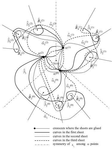
Figure 3. Homology basis of $\hat{X}$

Figure 4. $\varpi:\hat{X}\to X$

Up to homotopy, $\hat{\alpha}_{1}$ equals $\varpi\hat{\alpha}_{1}$; similarly $\varpi\hat{\beta}_{1}=\beta_{1}$. On the other hand for $i=2,3$, Figure 3 shows that

(10.3) $$\varpi(\alpha_{i}^{(c)})=\alpha_{i},\quad\varpi(\beta_{i}^{(c)})=\beta_{i},$$

$$\varpi^{-1}(\alpha_{i})=\hat{\alpha}_{i}^{(0)}+\hat{\alpha}_{i}^{(1)}+\hat{\alpha}_{i}^{(2)},\quad\varpi^{-1}(\beta_{i})=(\hat{\beta}_{i}^{(0)},\hat{\beta}_{i}^{(1)},\hat{\beta}_{i}^{(2)}).$$

Let the Jacobian associated with $\hat{X}$ be denoted by $\hat{{\mathcal{J}}}_{7}$ and a basis of holomorphic one-forms be given by

$$\hat{\nu^{I}}_{1}=\frac{dz}{w^{2}},\quad\hat{\nu^{I}}_{2}=\frac{zdz}{w^{2}},\quad\hat{\nu^{I}}_{3}=\frac{z^{2}dz}{w^{2}},\quad\hat{\nu^{I}}_{4}=\frac{dz}{w},\quad$$

$$\hat{\nu^{I}}_{5}=\frac{z^{3}dz}{w^{2}},\quad\hat{\nu^{I}}_{6}=\frac{zwdz}{w^{2}},\quad\hat{\nu^{I}}_{7}=\frac{z^{4}dz}{w^{2}}.\quad$$

We have removed the factor $3$ in the denominators for later convenience. The Abel map $\hat{w}:\Gamma_{\infty^{(0)}}\hat{X}\to{\mathbb{C}}^{7}$ defined by these holomorphic one forms is denoted by

$$\hat{w}(\Gamma_{P_{1},{\infty^{(0)}}},\ldots,\Gamma_{P_{n},{\infty^{(0)}}})=\sum_{i=1}^{n}\hat{w}(\Gamma_{P_{i},{\infty^{(0)}}}),\quad\hat{w}(\Gamma_{P_{i},{\infty^{(0)}}})=\int^{\Gamma_{P_{i},{\infty^{(0)}}}}\hat{\nu^{I}}.$$

Since $dx=3z^{2}dz$, we have the relation

$$\hat{\nu^{I}}_{1}=\varpi^{*}{\nu^{I}}_{1},\quad\hat{\nu^{I}}_{5}=\varpi^{*}{\nu^{I}}_{2},\quad\hat{\nu^{I}}_{6}=\varpi^{*}{\nu^{I}}_{3},\quad\varpi^{*}({\nu^{I}})=\begin{pmatrix}\hat{\nu^{I}}_{1}\\ \hat{\nu^{I}}_{5}\\ \hat{\nu^{I}}_{6}\\ \end{pmatrix}.$$

However we should note the $\hat{\zeta}_{3}$-action according to the covering defined by $z$:

Lemma 10.1.

The maps $\iota_{\zeta_{3}}$ and $\hat{\zeta}_{3}$ induce

$$\iota_{\zeta_{3}}\varpi^{*}({\nu^{I}})=\varpi^{*}(\hat{\zeta}_{3}{\nu^{I}})=\hat{\zeta}_{3}\varpi^{*}({\nu^{I}}).$$

We consider the projections of the extended Abel maps,

$$\hat{w}(\Gamma_{\hat{P},\infty^{(0)}})|_{\varpi^{*}{\nu^{I}}}=\int_{\Gamma_{\hat{P},\infty^{(0)}}}\varpi^{*}{\nu^{I}},$$

and we have the Lemma:

Lemma 10.2.

$$\int_{\gamma}\nu^{I}=\frac{1}{3}\int_{\hat{\gamma}}\varpi^{*}{\nu^{I}},\quad\hat{\gamma}=\varpi^{-1}\gamma,\quad\gamma=\beta_{1},\alpha_{i},(i=2,3),$$

$$\int_{\gamma}\nu^{I}=\int_{\hat{\gamma}}\varpi^{*}{\nu^{I}},\quad\gamma=\varpi\hat{\gamma},\quad\hat{\gamma}=\alpha_{1},\alpha_{i}^{(c)},\beta_{i}^{(c)},(i=2,3,c=0,1,2).$$

Proof.

For a neighborhood $U$ of a point in $\alpha_{i}$, we have $U^{(c)}$ $(c=0,1,2)$ such that $U=\varpi U^{(c)}$. Then $\varpi^{*}{\nu^{I}}|_{U^{(c)}}=\iota_{\zeta_{3}}^{c}\varpi^{*}{\nu^{I}}|_{U^{(0)}}$ and they cancel the phase difference between $\alpha_{i}^{(c)}$ and $\alpha_{i}^{(0)}$. Then we have

$$\begin{split}\int_{\hat{\beta}_{1}}\varpi^{*}{\nu^{I}}&=\left(\int_{\hat{B}_{2}^{(0)}}^{(0,0)}+\int_{(0,0)}^{\hat{B}_{2}^{(1)}}+\int_{\hat{B}_{2}^{(1)}}^{(0,0)}+\int_{(0,0)}^{\hat{B}_{2}^{(2)}}+\int_{\hat{B}_{2}^{(2)}}^{(0,0)}+\int_{(0,0)}^{\hat{B}_{2}^{(0)}}\right)\varpi^{*}{\nu^{I}}\\ &=\left(\int_{\beta_{1}}+\hat{\zeta}_{3}^{2}\int_{\hat{\zeta}_{3}\beta_{1}}+\hat{\zeta}_{3}\int_{\hat{\zeta}_{3}^{2}\beta_{1}}\right){\nu^{I}}=3\int_{\beta_{1}}{\nu^{I}}.\\ \end{split}$$

Here we used the fact that $\zeta_{3}+\zeta_{3}^{2}=-1$. Similarly

$$\begin{split}\int_{\varpi^{-1}\alpha_{i}}\varpi^{*}{\nu^{I}}&=\int_{\alpha_{i}^{(0)}+\alpha_{i}^{(1)}+\alpha_{i}^{(2)}}\varpi^{*}{\nu^{I}}=3\int_{\alpha_{i}}{\nu^{I}}.\\ \end{split}$$

∎

Then we have the period matrices for $\hat{X}$,

$$(\hat{\omega}^{\prime}):=\frac{1}{2}(\int_{\hat{\alpha}_{1}}\hat{\nu^{I}},\int_{\hat{\alpha}_{2}^{(0)}}\hat{\nu^{I}},\int_{\hat{\alpha}_{2}^{(1)}}\hat{\nu^{I}},\int_{\hat{\alpha}_{2}^{(2)}}\hat{\nu^{I}},\int_{\hat{\alpha}_{3}^{(0)}}\hat{\nu^{I}},\int_{\hat{\alpha}_{3}^{(1)}}\hat{\nu^{I}},\int_{\hat{\alpha}_{3}^{(2)}}\hat{\nu^{I}}),$$

$$(\hat{\omega}^{\prime\prime}):=\frac{1}{2}(\int_{\hat{\beta}_{1}}\hat{\nu^{I}},\int_{\hat{\beta}_{2}^{(0)}}\hat{\nu^{I}},\int_{\hat{\beta}_{2}^{(1)}}\hat{\nu^{I}},\int_{\hat{\beta}_{2}^{(2)}}\hat{\nu^{I}},\int_{\hat{\beta}_{3}^{(0)}}\hat{\nu^{I}},\int_{\hat{\beta}_{3}^{(1)}}\hat{\nu^{I}},\int_{\hat{\beta}_{3}^{(2)}}\hat{\nu^{I}}).$$

Using these, we have the lattice $\hat{\Lambda}$ in ${\mathbb{C}}^{7}$ and the Jacobian $\hat{\mathcal{J}}_{7}$ is: $\hat{\mathcal{J}}_{7}={\mathbb{C}}^{7}/\hat{\Lambda}$.

Lemmas 10.1 and 10.2 give the following proposition:

Proposition 10.3.

$$(\hat{\omega}^{\prime},\hat{\omega}^{\prime\prime})|_{\varpi^{*}{\nu^{I}}}=(\omega_{1}^{\prime},\omega_{2}^{\prime},\omega_{2}^{\prime},\omega_{2}^{\prime},\omega_{3}^{\prime},\omega_{3}^{\prime},\omega_{3}^{\prime},3\omega_{1}^{\prime\prime},\omega_{2}^{\prime\prime},\omega_{2}^{\prime\prime},\omega_{2}^{\prime\prime},\omega_{3}^{\prime\prime},\omega_{3}^{\prime\prime},\omega_{3}^{\prime\prime}).$$

In consequence, it is natural to introduce

$$\hat{\Lambda}^{\mathrm{al};(1,0)}:=\sum_{i=1}^{3}\left({\mathbb{Z}}\hat{\omega}^{\prime}_{\mathrm{al}^{(c)},i}+{\mathbb{Z}}\hat{\omega}^{\prime\prime}_{\mathrm{al}^{(0)},i}\right),$$

where

$$(\hat{\omega}^{\prime}_{\mathrm{al}^{(1,c)},i})_{i=1,2,3}:=\frac{1}{2}(\int_{\hat{\alpha}_{1}}\varpi^{*}{\nu^{I}},\int_{\hat{\alpha}_{2}^{(0)}+\hat{\alpha}_{2}^{(1)}+\hat{\alpha}_{2}^{(2)}}\varpi^{*}{\nu^{I}},\int_{\hat{\alpha}_{3}^{(0)}+\hat{\alpha}_{3}^{(1)}+\hat{\alpha}_{3}^{(2)}}\varpi^{*}{\nu^{I}}),$$

$$(\hat{\omega}^{\prime\prime}_{\mathrm{al}^{(1,0)},i})_{i=1,2,3}:=\frac{1}{2}(\int_{\hat{\beta}_{1}}\varpi^{*}{\nu^{I}},\int_{\hat{\beta}_{2}^{(c)}}\iota_{\zeta_{3}}^{c}\varpi^{*}{\nu^{I}},\int_{\hat{\beta}_{3}^{(c)}}\iota_{\zeta_{3}}^{c}\varpi^{*}{\nu^{I}}).$$

On the other hand, we introduce a natural subvariety of $\hat{\mathcal{J}}_{7}$ as follows:

Definition 10.4.

For the projection of the extended Abel map,

$$\hat{w}|_{\varpi^{*}{\nu^{I}}}:S^{3}\Gamma_{\infty^{(0)}}\hat{X}\to{\mathbb{C}}^{3}\subset{\mathbb{C}}^{7},$$

${\hat{\mathcal{J}}}^{\mathrm{al};(1,0)}$ is defined by

$${\hat{\mathcal{J}}}^{\mathrm{al};(1,0)}:=\frac{\hat{w}(S^{3}\Gamma_{\infty^{(0)}}\hat{X})|_{\varpi^{*}{\nu^{I}}}}{\hat{\Lambda}_{\mathrm{al}^{(1,0)}}},$$

for $c=0,1,2$.

Then ${\hat{\mathcal{J}}}^{\mathrm{al};(1,0)}\subset\hat{{\mathcal{J}}}$ is the domain of the $\mathrm{al}_{1}$-function,

$$\hat{\mathrm{al}}_{1}(u):=\frac{1}{z_{1}z_{2}z_{3}}\frac{\left|\begin{matrix}1&z_{1}^{3}&w_{1}z_{1}&z_{1}^{6}\\ 1&z_{2}^{3}&w_{2}z_{2}&z_{2}^{6}\\ 1&z_{3}^{3}&w_{3}z_{3}&z_{3}^{6}\\ 1&b_{a}&0&b_{a}^{2}\\ \end{matrix}\right|}{\left|\begin{matrix}1&z_{1}^{3}&w_{1}z_{1}\\ 1&z_{2}^{3}&w_{2}z_{2}\\ 1&z_{3}^{3}&w_{3}z_{3}\\ 1&b_{a}&0\\ \end{matrix}\right|},$$

where $u=\sum_{i=1}^{3}\hat{w}((z_{i},w_{i}))|_{\varpi^{*}{\nu^{I}}}$ for $((z_{i},w_{i}))_{i=1,2,3}\in S^{3}\hat{X}$.

Finally we have the following proposition.

Proposition 10.5.

1. $\hat{w}((z_{i},w_{i}))|_{\varpi^{*}{\nu^{I}}}$ is surjective.

2. There is an equality

   $$\hat{\mathrm{al}}_{1}(u)=\varpi^{*}\mathrm{al}_{1}^{(0)}(u).$$

3. By identifying $\hat{w}(S^{3}\hat{X})|_{\varpi^{*}{\nu^{I}}}={\mathbb{C}}^{3}$ with $w(S^{3}X)={\mathbb{C}}^{3}$, ${\hat{\mathcal{J}}}^{\mathrm{al},(1,0)}$ agrees with ${\hat{\mathcal{J}}}^{(1;0)}$.

A. Appendix: Hyperelliptic $\mathrm{al}$ Functions

In this appendix, we review the hyperelliptic $\mathrm{al}$-function mainly following [Ba1, Ba2].

Hyperelliptic Curve: We let a (hyper)elliptic curve $C_{g}$ of genus $g$ $(g>0)$ be defined by the affine equation,

(A.1) $$\begin{split}y^{2}&=(x-b_{0})(x-b_{1})(x-b_{2})\cdots(x-b_{2g})\\ &=P(x)Q(x),\end{split}$$

where $b_{j}$’s are distinct complex numbers, $P(x)=(x-b_{1})(x-b_{3})\cdots(x-b_{2g-1})$ and $Q(x):=y^{2}/P(x)$. Let $(b_{j},0)=B_{j}\in C_{g}$.

For a point $(x,y)\in C_{g}$, differentials of the first kind (not normalized in the standard way which gives the identity as the matrix of $A$-periods) are defined by,

$${\nu^{I}}_{i}:=\frac{x^{i-1}dx}{2y}.$$

The extended Abel map from the $g$-th symmetric product of the universal cover $\Gamma_{\infty}C_{g}$ of the curve $C_{g}$ to ${\mathbb{C}}^{g}$ is defined by,

$$w:{S}^{g}\Gamma_{\infty}C_{g}\longrightarrow\mathbb{C}^{g},\quad\left(w(\Gamma_{(x_{1},y_{1}),\infty},\ldots,\Gamma_{(x_{g},y_{g}),\infty}):=\sum_{i=1}^{g}\int_{\Gamma_{(x_{g},y_{g}),\infty}}{\nu^{I}}\right),$$

where $\Gamma_{(x_{g},y_{g}),\infty}$ is a path in the path space $\Gamma_{\infty}C_{g}$.

Consider $\mathrm{H}_{1}(C_{g},\mathbb{Z})=\bigoplus_{j=1}^{g}\mathbb{Z}\alpha_{j}\oplus\bigoplus_{j=1}^{g}\mathbb{Z}\beta_{j},$ the homology group of the hyperelliptic curve $C_{g}$, where the intersections are given by $[\alpha_{i},\alpha_{j}]=0$, $[\beta_{i},\beta_{j}]=0$ and $[\alpha_{i},\beta_{j}]=\delta_{i,j}$. Here we employ the choice illustrated in Figure 5.

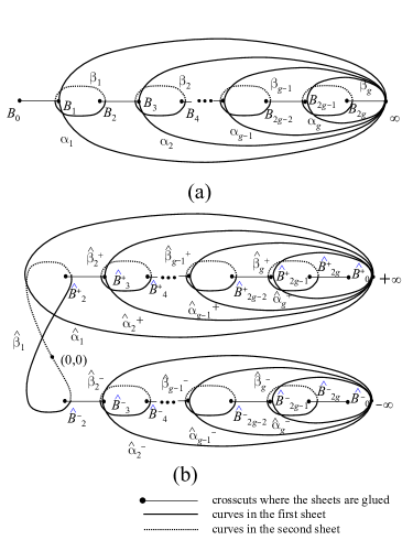
Figure 5. (a): $C_{g}$ and (b): $\hat{C}_{2g-1}$

The (half-period) hyperelliptic integrals of the first kind are defined by,

$${\omega}^{\prime}:=\frac{1}{2}\left[\left(\int_{\alpha_{j}}{\nu^{I}}_{i}\right)_{ij}\right],\quad{\omega}^{\prime\prime}:=\frac{1}{2}\left[\left(\int_{\beta_{j}}{\nu^{I}}_{i}\right)_{ij}\right],\quad{\omega}:=\left[\begin{matrix}{\omega}^{\prime}\\ {\omega}^{\prime\prime}\end{matrix}\right].$$

If we let:

$$\omega_{a}:=\int^{B_{a}}_{\infty}{\nu^{I}},\quad(a=0,1,2,\cdots,2g-1,2g),$$

Figure 5 shows:

$$\omega^{\prime}_{a}=\omega_{2a-1},\quad\omega^{\prime\prime}_{a}=\omega_{2a}-\omega_{2a-1},\quad a>1.$$

The Jacobian ${\mathcal{J}}_{g}$ is defined as the complex torus,

$${\mathcal{J}}_{g}:=\mathbb{C}^{g}/{{\Lambda}}_{g}.$$

Here ${\Lambda}_{g}$ is a $2g$-dimensional lattice generated by the period matrix given by $2{\omega}$. We also use the same letter $u$ for a vector in $\mathbb{C}^{g}$ and a point of the Jacobian ${\mathcal{J}}_{g}$.

Using the (unnormalized) differentials of the second kind,

$${\nu^{II}}_{j}={\displaystyle\frac{1}{2y}}\sum_{k=j}^{2g-j}(k+1-j)\lambda_{k+1+j}x^{k}dx,\quad(j=1,\ldots,g),$$

the half-period hyperelliptic matrices of the second kind are defined by,

$${\eta}^{\prime}:=\frac{1}{2}\left[\left(\int_{\alpha_{j}}{\nu^{II}}_{i}\right)_{ij}\right],\quad{\eta}^{\prime\prime}:=\frac{1}{2}\left[\left(\int_{\beta_{j}}{\nu^{II}}_{i}\right)_{ij}\right].$$

The hyperelliptic $\sigma$ function, which is a holomorphic function over $u\in\mathbb{C}^{g}$, is defined by [[Ba2], p.336, p.350], [Kl, BEL2],

(A.2) $$\sigma(u):=\sigma(u;C_{g}):=\ \gamma\mathrm{exp}(-{\displaystyle\frac{1}{2}}\ ^{t}\ u{\eta}^{\prime}{{\omega}^{\prime}}^{-1}u)\vartheta\negthinspace\left[\begin{matrix}\delta^{\prime\prime}\\ \delta^{\prime}\end{matrix}\right](\frac{1}{2}{{\omega}^{\prime}}^{-1}u;\tau),$$

where $\gamma$ is a certain constant factor, $\vartheta\left[\negthinspace\right]$ is the Riemann $\theta$ function with characteristics,

$$\vartheta\negthinspace\left[\begin{matrix}a\\ b\end{matrix}\right](z;\tau):=\sum_{n\in\mathbb{Z}^{g}}\exp\left[2\pi\sqrt{-1}\left\{{\displaystyle\frac{1}{2}}\ ^{t}\negthinspace(n+a)\tau(n+a)+\ ^{t}\negthinspace(n+a)(z+b)\right\}\right],$$

with $\tau:={{\omega}^{\prime}}^{-1}{\omega}^{\prime\prime}$ for $g$-dimensional vectors $a$ and $b$, and

$$\delta^{\prime}:=\ ^{t}\left[\begin{matrix}{\displaystyle\frac{g}{2}}&{\displaystyle\frac{g-1}{2}}&\cdots&{\displaystyle\frac{1}{2}}\end{matrix}\right],\quad\delta^{\prime\prime}:=\ ^{t}\left[\begin{matrix}{\displaystyle\frac{1}{2}}&\cdots&{\displaystyle\frac{1}{2}}\end{matrix}\right].$$

Proposition A.1.

If for $u$, $v\in{\mathbb{C}}^{3}$, and $\ell$ ($=2\omega^{\prime}\ell^{\prime}+2\omega^{\prime\prime}\ell^{\prime\prime}$) $\in\Lambda$, we define

$$L(u,v) :=2{}^{t}{u}(\eta^{\prime}v^{\prime}+\eta^{\prime\prime}v^{\prime\prime}),$$

$$\chi(\ell) :=\exp[\pi\sqrt{-1}\big{(}2({}^{t}{\ell^{\prime}}\delta^{\prime\prime}-{}^{t}{\ell^{\prime\prime}}\delta^{\prime})+{}^{t}{\ell^{\prime}}\ell^{\prime\prime}\big{)}]\ (\in\{1,\,-1\}),$$

the following holds

$$\sigma(u+\ell)=\sigma(u)\exp(L(u+\frac{1}{2}\ell,\ell))\chi(\ell).$$

Definition A.2.

1. We define the double coverings of ${\mathcal{J}}_{g}$ by

   $${\mathcal{J}}_{g}^{(a)}={\mathbb{C}}^{g}/\Lambda^{(a)},$$

   where $\Lambda^{(0)}:=\bigcap_{a=1}^{2g}\Lambda^{(a)}$,

   $$\begin{split}\Lambda^{(a)}:=&2{\mathbb{Z}}\omega^{\prime}_{a}+4{\mathbb{Z}}\omega^{\prime\prime}_{a}+\sum_{b=1,\neq a}(2{\mathbb{Z}}\omega^{\prime}_{b}+2{\mathbb{Z}}\omega^{\prime\prime}_{b})\quad\mbox{for }a=1,3,\ldots,2g-1,\\ \Lambda^{(a)}:=&4{\mathbb{Z}}\omega^{\prime}_{a}+4{\mathbb{Z}}\omega^{\prime\prime}_{a})+\sum_{b=1,\neq a}(2{\mathbb{Z}}\omega^{\prime}_{b}+2{\mathbb{Z}}\omega^{\prime\prime}_{b})\quad\mbox{for }a=2,4,\ldots,2g.\\ \end{split}$$

2. For a point $\Gamma_{P_{c},\infty}\in\Gamma_{\infty}C_{g}$,

   $$\varepsilon_{r}^{(c)}:\Gamma_{\infty}C_{g}\to{\mathbb{Z}}_{2}$$

   be defined by $\varepsilon_{r}^{(c)}:=w_{r}-w_{\infty}$ for the winding number $w_{r}$ around $B_{a}$ in $\kappa_{\infty}\Gamma_{\infty}C_{g}$ and the winding number $w_{\infty}$ around $\infty$ in $\kappa_{\infty}\Gamma_{\infty}C_{g}$. For a point $(\Gamma_{P_{1},\infty},\Gamma_{P_{2},\infty},\ldots,\Gamma_{P_{g},\infty})$ in $S^{g}\Gamma_{\infty}C_{g}$, let

   $$\varepsilon_{r}:S^{g}\Gamma_{\infty}C_{g}\to{\mathbb{Z}}_{2},\quad(\varepsilon_{r}:=\varepsilon_{r}^{(1)}+\varepsilon_{r}^{(2)}+\cdots+\varepsilon_{r}^{(g)}).$$

3. For a point $(\Gamma_{P_{1},\infty},\Gamma_{P_{2},\infty},\ldots,\Gamma_{P_{g},\infty})$ in $S^{g}\Gamma_{\infty}C_{g}$, let $u=w(\Gamma_{P_{1},\infty},\Gamma_{P_{2},\infty},\ldots,\Gamma_{P_{g},\infty})$. The hyperelliptic $\mathrm{al}$ function over ${\mathcal{J}}^{(r)}$ and $w^{-1}{\mathcal{J}}^{(r)}$ as a subset of a quotient space of in $S^{g}\Gamma_{\infty}C_{g}$, is formally defined by [Ba2, p.340], [Wei],

   (A.3) $$\mathrm{al}_{r}(u):=(-1)^{\varepsilon_{r}(\Gamma_{\infty,P_{1}},\Gamma_{\infty,P_{2}},\ldots,\Gamma_{\infty,P_{g}})}\sqrt{F(b_{r})},$$

   where

   (A.4) $$F(x):=(x-x_{1})\cdots(x-x_{g}),$$

   for a preimage $(\Gamma_{(x_{i},y_{i}),\infty})_{i=1,\ldots,g}\in S^{g}\Gamma_{\infty}C_{g}$ of $w((\Gamma_{(x_{i},y_{i}),\infty})_{i=1,\ldots,g})=u\in{\mathcal{J}}^{(r)}$ under the Abel map.

Remark A.3.

The definition (A.3) is historically

(A.5) $$\mathrm{al}_{r}(u)=\tilde{\gamma}_{r}\sqrt{F(b_{r})},$$

where $\tilde{\gamma}_{r}:=\sqrt{-1/P^{\prime}(b_{r})}$. Thus the preimage of $w$ of ${\mathcal{J}}^{(r)}$ is a quotient space of $S^{g}\Gamma_{\infty}C_{g}$. We comment on the sign $(-1)^{\varepsilon}$ in the right-hand side of (A.3). The hyperelliptic curve $C_{g}$ admits the hyperelliptic involution $\iota_{H}:(x,y)\to(x,-y)$. In a neighborhood of the branch point $B_{r}=(b_{r},0)$, $y$ or $t$ such that $t^{2}=(x-b_{r})$ are local parameters. Thus for $t_{i}$ such that $t_{i}^{2}:=(x_{i}-b_{r})$ $\iota_{H}^{(a)}t_{i}=-t_{i}$. Similarly, $t_{1}t_{2}\cdots t_{g}$ is defined in a neighborhood of $B_{r}$ and $\iota_{H}$ can be made to act on the product: a circuit around the point produces the factor $(-1)^{\varepsilon_{r}(\Gamma_{\infty,P_{1}},\Gamma_{\infty,P_{2}},\ldots,\Gamma_{\infty,P_{g}})}$.

Further the inverse $1/t_{i}$ is a local parameter at $\infty$ and thus there is an action $\iota_{H}^{(\infty)}(1/t_{i})=-(1/t_{i})$, and a circuit around $\infty$ generates $(-1)^{\varepsilon_{r}(\Gamma_{\infty,P_{1}},\Gamma_{\infty,P_{2}},\ldots,\Gamma_{\infty,P_{g}})}$.

However we claim that we can make sense of $t_{1}t_{2}\cdots t_{g}$ globally and (A.5) holds globally by (A.3). In analogy to Jacobi’s sn, cn, dn functions, we need to extend the domain of the Jacobi inversion from ${\mathcal{J}}_{g}$ to ${\mathcal{J}}_{g}^{(r)}$ and ${\mathcal{J}}_{g}^{(0)}$. We show the extension in Proposition A.10; here we consider the behavior of the right-hand side of (A.3). Let us regard it as a function of $w(P_{1})$ by fixing $P_{2}$, $\ldots$, $P_{g}$. Then a circuit around $\alpha_{b}$ (see Figure 5 (a)) does not have any effect on the sign factor of $t_{1}$. On the other hand, when we go around $\beta_{a}$ in Figure 5 (a) once, $t_{1}$ acquires a sign and in order to cancel it, we need to go twice around $\beta_{a}$. Thus the (homotopy) equivalence relation is the same as that which holds for ${\mathcal{J}}_{g}^{(a)}$.

Proposition A.4.

Introducing the half-period $\omega_{r}:=\int^{b_{r}}_{\infty}du$, we have the relation [Ba2, 340],

(A.6) $$\mathrm{al}_{r}(u)=\gamma_{r}^{\prime\prime}\frac{\exp(-{}^{t}u\varphi_{r})\sigma(u+\omega_{r})}{\sigma(u)},\quad r=1,2,\ldots,2g,$$

where $\gamma_{r}^{\prime\prime}$ is a certain constant.

$$\varphi_{r}=\left\{\begin{matrix}{\eta}^{\prime}{{\omega}^{\prime}}^{-1}\omega^{\prime}_{r}&r=1,3,\ldots,2g-1,\\ {\eta}^{\prime\prime}{{\omega}^{\prime\prime}}^{-1}\omega^{\prime\prime}_{r}+{\eta}^{\prime}{{\omega}^{\prime}}^{-1}\omega^{\prime}_{r}&r=2,4,\ldots,2g.\\ \end{matrix}\right.$$

Proof.

By comparing zeros and poles of both sides, we have the result. ∎

Proposition A.5.

For a lattice point $\ell$ in $\Lambda^{(b)}$

$$\mathrm{al}_{b}(u)=\mathrm{al}_{b}(u+\ell).$$

Proof.

We know:

$$\frac{\sigma(u+\omega_{b}+\ell)}{\sigma(u+\ell)}=\frac{\sigma(u+\omega_{b})}{\sigma(u)}\exp(L(\omega_{b},\ell)).$$

For the $b=2a-1$ case,

(A.7) $$\begin{split}L(\omega_{b}^{\prime},\ell)&=2^{t}\omega_{b}^{\prime}(\eta^{\prime}\ell^{\prime}+\eta^{\prime\prime}\ell^{\prime\prime})\\ &=2^{t}\omega_{b}^{\prime}\eta^{\prime}\ell^{\prime}+2^{t}\omega_{b}^{\prime\prime}\eta^{\prime}\ell^{\prime\prime}-\pi{\sqrt{-1}}\ell^{\prime\prime}_{b},\\ \end{split}$$

whereas

(A.8) $$2^{t}(\omega^{\prime}\ell^{\prime}+\omega^{\prime\prime}\ell^{\prime\prime})\eta^{\prime}\omega^{\prime-1}\omega_{b}^{\prime}=2^{t}\ell^{\prime}{}^{t}\eta^{\prime}\omega_{b}^{\prime}+2{}^{t}\ell^{\prime\prime}\omega_{b}^{\prime\prime}\eta^{\prime}.$$

Hence we have the equality. ∎

As a generalization of the relation $\mathrm{sn}^{2}u+\mathrm{cn}^{2}u=1$, we have the following relation.

Proposition A.6.

Let $A_{a}(x)=P(x)(x-b_{a})$ and $a\in\{2,4,\ldots,2g\}$.

$$\sum_{r=1,3,\ldots,2g-1,a}\frac{\mathrm{al}_{r}(x)^{2}}{A^{\prime}_{a}(b_{r})}=1.$$

Proof.

See [Wei, p.292] and also [Ma4, Proposition 3.4]. ∎

Remark A.7.

The relation implies the $g$ homogeneous identities,

$$\sum_{r=1,3,\ldots,2g-1,a}\frac{(\gamma_{r}^{\prime\prime})^{2}\mathrm{e}^{-2{}^{t}u\varphi_{r}}}{A^{\prime}_{a}(b_{r})}\sigma(u+\omega_{r})^{2}\equiv\sigma(u)^{2},\quad a=2,4,\ldots,2g,$$

among $2g+1$ homogeneous coordinates, namely, $\sigma(u+\omega_{r})$ ($r=1,2,\ldots,2g$) and $\sigma(u)$. Noting that the square of each $\mathrm{al}_{r}$ is a function over the hyperelliptic Jacobi variety ${\mathcal{J}}_{g}$, these quadrics cut out the image of the Jacobian, which is a $g$-dimensional variety embedded in $\mathbb{P}^{2g}$.

Remark A.8.

For the genus-one case, the Weierstrass $\wp$ function corresponds to a curve $y^{2}=(x-e_{1})(x-e_{2})(x-e_{3})$, whereas the Jacobi $\mathrm{sn}$ functions is defined on:

(A.9) $$w^{2}=(z^{2}-1)(z^{2}-k^{2}),$$

where $w=y/z\sqrt{(e_{2}-e_{1})^{3}}$, $z=\sqrt{(x-e_{1})/(e_{2}-e_{1})}$ and

$$\frac{dx}{2y}=2\sqrt{e_{2}-e_{1}}\frac{dz}{2w}.$$

We have employed a curve (A.1) with $f(x)$ of odd degree (thus a branchpoint at $\infty$), and the associated $\wp_{ij}$ function.

Note that when $g=1$, (A.10) is essentially reduced to (A.9).

Given that the $\mathrm{al}_{r}$ function is a generalization of the $\mathrm{sn}$-function, we considered a genus $2g-1$ curve $\hat{C}_{2g-1}$ whose affine part is given by

(A.10) $$w^{2}=\prod_{i=1,\neq r}^{2g+1}(z^{2}-a_{i}),$$

where $a_{i}=b_{i}-b_{r}$, $z=\sqrt{x-b_{r}}$, and $w=y/z$.

Let $(b_{i},0)=B_{i}\in C_{g}$ be the branch points on the affine plane and $(x,y)\in C_{g}$ be a general point $P$. For $c_{i}^{2}:=a_{i}$, let $(\pm c_{i},0)\in\hat{C}_{2g-1}$ be $\hat{B}_{i}^{\pm}$ as a finite branch point and $(z,w)\in C_{g}$ be a general point $\hat{P}^{\pm}$.

There is an involution $\iota_{A}:(z,w)\mapsto(-z,w)$ as well as the hyperelliptic involution $\hat{\iota}_{H}:(z,w)\mapsto(z,-w)$ and $\iota_{H}:(x,y)\mapsto(x,-y)$.

At the point $\infty$ of $\hat{C}_{2g+1}$, acting by $\iota_{H}$ and $\iota_{A}$, we identify the actions $\hat{\iota}_{H}$ and $\iota_{A}$, i.e.,

$$\hat{\iota}_{H}:\pm\infty\mapsto\mp\infty,\quad\iota_{A}:\pm\infty\mapsto\mp\infty.$$

On the other hand $(0,0)\in\hat{C}_{2g+1}$, which corresponds to $B_{r}\in C_{g}$ is the fixed point of $\hat{\iota}_{H}$ and $\iota_{A}$.

Let us consider the $r=1$ case. Then there is a double covering:

$$\varpi_{g}:\hat{C}_{2g-1}\to C_{g},\quad(\hat{P}=(z,w)\mapsto P=(z^{2}+b_{r},wz)),$$

and

$$(0,0)\mapsto B_{1},\quad\hat{B}_{i}^{\pm}\to B_{i},\quad(i=2,3,\cdots,2g,2g+1).$$

We illustrate this in Figure 6, which is essentially the same as the picture in [ACGH, p.296].

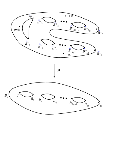
Figure 6. $\varpi:\hat{C}_{2g-1}\to C_{g}$

The (unnormalized) basis of holomorphic one-forms over $\hat{C}_{2g-1}$ is denoted by

$$\hat{\nu^{I}}:=\begin{pmatrix}\hat{\nu^{I}}_{1}\\ \hat{\nu^{I}}_{2}\\ \vdots\\ \hat{\nu^{I}}_{2g-1}\\ \end{pmatrix},\quad\hat{\nu}^{I}_{j}=\frac{z^{j-1}dz}{w},\quad(j=1,2,\ldots,2g-1).$$

Here we have removed the factor $1/2$ for later convenience. Let us consider the Abel map

$$\hat{w}:{S}^{k}\Gamma_{-\infty}\hat{C}_{2g-1}\longrightarrow{\mathbb{C}}^{2g-1},\quad\left(\hat{w}(\Gamma_{(x_{1},y_{1}),-\infty},\ldots,\Gamma_{(x_{k},y_{k}),-\infty}):=\sum_{i=1}^{k}\int_{\Gamma_{(x_{i},y_{i}),-\infty}}\hat{\nu^{I}}\right).$$

As the contours in Figure 5 (b) illustrate, the associated periodic matrices are given as,

$$(\hat{\omega}^{\prime},\hat{\omega}^{\prime\prime}):=\frac{1}{2}\left(\left(\int_{\hat{\alpha}_{1}}\hat{\nu^{I}},\left(\int_{\hat{\alpha}_{i}^{+}}\hat{\nu^{I}},\int_{\hat{\alpha}_{i}^{-}}\hat{\nu^{I}}\right)_{i=2,\ldots,g}\right),\left(\int_{\hat{\beta}_{1}}\hat{\nu^{I}},\left(\int_{\hat{\beta}_{i}^{+}}\hat{\nu^{I}},\int_{\hat{\beta}_{i}^{-}}\hat{\nu^{I}}\right)_{i=2,\ldots,g}\right)\right).$$

The lattice associated with the curve $\hat{C}_{2g-1}$ is denoted by $\hat{\Lambda}$ and its Jacobian by $\hat{\mathcal{J}}_{2g-1}={\mathbb{C}}^{2g-1}/\hat{\Lambda}$.

Direct computations show the following facts:

Proposition A.9.

1. $$\frac{z^{2i-2}dz}{w}=\frac{x^{i-1}dx}{2y},\quad(i=1,\ldots,g),\quad\varpi^{*}{\nu^{I}}=\begin{pmatrix}\hat{\nu^{I}}_{1}\\ \hat{\nu^{I}}_{3}\\ \vdots\\ \hat{\nu^{I}}_{2g-1}\\ \end{pmatrix}.$$

2. $$\hat{\iota}_{H}\varpi^{*}{\nu^{I}}=\varpi^{*}\iota_{H}{\nu^{I}}=\hat{\iota}_{A}\varpi^{*}{\nu^{I}}.$$

3. By defining

   $$\left(\sum_{i}^{g}\int_{\Gamma_{(x_{i},y_{i}),-\infty}}\varpi^{*}{\nu^{I}}\right),$$

   $\hat{w}_{\varpi^{*}{\nu^{I}}}:S^{g}\Gamma_{-\infty}\hat{C}_{2g-1}\to{\mathbb{C}}^{g}$ is a surjection.

Figure 5 shows that as half of $\beta_{1}$ consists of the path from $\infty$ to $B_{1}$, the path from $\pm\infty$ to $(0,0)$ in $\hat{C}_{2g-1}$ corresponds to a quarter of $\hat{\beta}_{1}$. Each $\hat{\beta}_{a}^{\pm}$ $(a=2,\ldots,g)$ consists of a contour from $\pm\infty$ to $\hat{B}_{2a-1}^{\pm}$. Similarly we have $\hat{\alpha}_{a}^{\pm}$ $(a=1,\ldots,g)$.

Noting that $({B_{1}}\to B_{2})$ lifts to $(0,0)\to\hat{B}_{2}^{(\pm)})$, we find that

$$\int^{B_{2}}_{B_{1}}\nu^{I}=\frac{1}{2}\int^{\hat{B}_{2}}_{(0,0)}\varpi^{*}\nu^{I}$$

is a half-period in $\hat{C}_{2g-1}$. The $(2(2g-1)\times g)$ matrix $(\hat{\omega}^{\prime},\hat{\omega}^{\prime\prime})|_{\varpi{\nu^{I}}}$ is given by

$$(\omega^{\prime}_{1},\omega_{2}^{\prime},\omega_{2}^{\prime},\ldots,\omega_{g}^{\prime},\omega_{g}^{\prime},2\omega^{\prime\prime}_{1},\omega_{2}^{\prime\prime},\omega_{2}^{\prime\prime},\ldots,\omega_{g}^{\prime\prime},\omega_{g}^{\prime\prime}).$$

The corresponding lattice is denoted by $\hat{\Lambda}$ and the Jacobian by $\hat{\mathcal{J}}={\mathbb{C}}^{2g-1}/\hat{\Lambda}$.

Proposition A.10.

Let

$${\hat{\mathcal{J}}}^{\mathrm{al},(1)}_{g}:=\frac{\hat{w}_{\varpi^{*}{\nu^{I}}}(S^{g}\Gamma_{-\infty}\hat{C}_{2g-1})}{\hat{\Lambda}\cap\hat{w}_{\varpi^{*}{\nu^{I}}}(S^{g}\Gamma_{-\infty}\hat{C}_{2g-1})}.$$

Then the following function is defined on ${\hat{\mathcal{J}}}^{\mathrm{al},(1)}_{g}$,

$$(z_{1}z_{2}\cdots z_{g})(u),$$

where $(z_{1},z_{2},\ldots,z_{g})$ in $S^{g}\Gamma_{-\infty}\hat{C}_{2g-1}$ is any preimage of $u$ under the extended Abel map.

By identifying $w(S^{g}\Gamma_{\infty}C_{g})={\mathbb{C}}^{g}$ and $\hat{w}_{\varpi^{*}{\nu^{I}}}(S^{g}\Gamma_{-\infty}\hat{C}_{2g-1})={\mathbb{C}}^{g}$, ${\hat{\mathcal{J}}}^{\mathrm{al},(1)}_{g}$ and ${{\mathcal{J}}}^{(1)}_{g}$ agree, and their $\mathrm{al}_{1}$ function is expressed by

$$\mathrm{al}_{1}(u)=(z_{1}z_{2}\cdots z_{g})(u).$$

Shigeki Matsutani
8-21-1 Higashi-Linkan Minami-ku,
Sagamihara 252-0311,
JAPAN.
rxb01142@nifty.com

Emma Previato
Department of Mathematics and Statistics,
Boston University,
Boston, MA 02215-2411,
U.S.A.
ep@bu.edu

References

[ACGH]
E. Arbarello, M. Cornalba, P. A. Griffiths, and J. Harris,
Geometry of Algebraic Curves Volume I,
Springer,
(1984) .
[AHP]
M. R. Adams, J. Harnad, and E. Previato,
Isospectral Hamiltonian flows in finite and infinite dimensions. I.
Generalized Moser systems and moment maps into loop algebras,
Comm. Math. Phys.,
117 (1988) 451-500.
[Ba1]
H.F. Baker,
Abelian functions. Abel’s theorem and the allied theory of
theta functions,
Reprint of the 1897 original.
With a foreword by Igor Krichever.
Cambridge Mathematical Library. Cambridge University Press, Cambridge, 1995.
[Ba2]
H. F. Baker,
On the hyperelliptic sigma functions,
Amer. J. of Math.,
XX
(1898)
301-384.
[Ba3]
H. F. Baker,
On a system of differential equations
leading to periodic functions,
Acta Math.,
27
(1903)
135-156.
[BEL1]
V. M. Buchstaber, V. Z. Enolskii, and D. V. Leykin,
Kleinian Functions,
Hyperelliptic Jacobians and Applications,
Reviews in Mathematics and Mathematical Physics (London),
eds.Novikov, S. P. and Krichever, I. M.
Gordon and Breach, India, (1997)
1-125.
[BEL2]
V. M. Buchstaber, V. Z. Enolskii, and D. V. Leykin,
Uniformization of Jacobi Varieties of Trigonal Curves and Nonlinear
Differential Equation,
Funct. Anal. Appl., 34 (2000) 159-171.
[BLE]
V. M. Buchstaber, D. V. Leykin, and V. Z. Enolskii,
-function of -curves,
Russian Math. Surveys, 54 (1999) 628-629.
[C]
M. Cornalba,
On the locus of curves with automorphisms, ,
Ann. Mat. Pura Appl.,
149 (1987) 135-151.
[EEL]
J. C. Eilbeck, V. Z. Enolskii and D. V. Leykin,
On the Kleinian construction of Abelian
functions of canonical algebraic curves,
In Proceedings of the Conference SIDE III:
Symmetries of Integrable Differences Equations, Saubadia, May 1998,
CRM Proceedings and Lecture Notes, ,
(2000)
121-138
[EEMÔP1]
J.C. Eilbeck, V.Z. Enolskii, S. Matsutani,
Y. Ônishi and E. Previato,
Addition formulae over the Jacobian pre-image of
hyperelliptic Wirtinger varieties ,
J. reine angew. Math., 619 (2008), 37-48.