Smooth Projective Toric Variety Representatives in Complex Cobordism

Abstract.

A general problem in complex cobordism theory is to find useful representatives for cobordism classes. One particularly convenient class of complex manifolds consists of smooth projective toric varieties. The bijective correspondence between these varieties and smooth polytopes allows us to examine which complex cobordism classes contain a smooth projective toric variety by studying the combinatorics of polytopes. These combinatorial properties determine obstructions to a complex cobordism class containing a smooth projective toric variety. However, the obstructions are only necessary conditions, and the actual distribution of smooth projective toric varieties in complex cobordism appears to be quite complicated. The techniques used here provide descriptions of smooth projective toric varieties in low-dimensional cobordism.

1. Introduction

In 1958, Hirzebruch posed the following question regarding complex cobordism [15].

Question 1.1.

Which complex cobordism classes can be represented by connected smooth algebraic varieties?

Practically no progress has been made on this difficult problem. The best that has been achieved is an understanding of complex cobordism representatives which display some of these properties. For example, Milnor demonstrated that each complex cobordism class can be represented by a smooth not necessarily connected algebraic variety [28, Chapter VII]. In 1998, Buchstaber and Ray addressed a toric version of Hirzebruch’s question. They demonstrated that every complex cobordism class can be represented by a topological generalization of a toric variety called a quasitoric manifold [4, 6]. These representatives are smooth and connected, but they are not algebraic varieties.

Another way of approaching Hirzebruch’s question could be to focus on a more specific collection of connected smooth algebraic varieties and study their cobordism classes. In particular, smooth projective toric varieties display a convenient combinatorial structure which aids in computations, including complex cobordism computations. It would seem reasonable to expect that the additional structure of smooth projective toric varieties would make the following question easier to answer than Hirzebruch’s original question.

Question 1.2.

Which complex cobordism classes can be represented by smooth projective toric varieties?

Answering this question would at least give some information regarding Hirzebruch’s original question, since these algebraic varieties are all smooth and connected. Unfortunately, even this simpler question seems to have a complex and nuanced answer. In what follows, we will examine Question 1.2 in low-dimensional cobordism. A complete description of cobordism classes containing smooth projective toric varieties will be provided up to dimension six. Describing smooth projective toric variety representatives in dimensions eight and higher is already significantly more complicated, so only partial descriptions will be provided in these dimensions.

The cobordism of smooth projective toric varieties will be studied by examining certain properties of convex geometric objects like fans and polytopes that are associated to the toric varieties. Section 2 will provide a brief introduction to the material involving complex cobordism and toric varieties that is needed to approach Question 1.2.

One well-known obstruction to a cobordism class containing a smooth toric variety is its Todd genus. More specifically, the Todd genus of a smooth toric variety must equal one [17]. In the case of smooth projective toric varieties, this is just one of several obstructions that arise from the combinatorial structure of the corresponding polytopes. In Section 3, we discuss these more generalized combinatorial obstructions.

In Section 4, we determine the obstructions to a cobordism class containing a smooth projective toric variety in $\Omega_{2}^{U}$ and $\Omega_{4}^{U}$. In these dimensions, the combinatorial restrictions happen to be the only obstructions.

In Section 5, we examine this representation problem in $\Omega_{6}^{U}$. In this dimension, there are additional obstructions to a cobordism class containing a smooth projective toric variety. A classification theorem for smooth polyhedra and an explicit construction will be used to describe all complex cobordism classes in this dimension that contain a smooth projective toric variety.

In Section 6, we examine Question 1.2 in $\Omega_{8}^{U}$. The results in this dimension are much more complicated, so only a partial description can be provided. As in $\Omega_{6}^{U}$, there are additional obstructions besides those arising from the combinatorial structure of smooth projective toric varieties. However, if certain parameters are chosen to provide sufficient freedom (more specifically, by choosing smooth projective toric varieties whose associated polytopes have specified $g$-vectors), then these combinatorial obstructions are the only obstructions in $\Omega_{8}^{U}$.

Section 7 presents some final thoughts on how these partial answers to Question 1.2 could be generalized and improved. Approaching this problem from several different angles could potentially provide more complete results in the future.

2. Background

In order to understand the role that smooth projective toric varieties play in complex cobordism, we must first establish some basic facts and techniques regarding each of these.

2.1. Chern Numbers of Complex Cobordism Classes

Milnor and Novikov proved that any complex cobordism class in $\Omega_{2n}^{U}$ is completely described by its list of $\left|\pi\left(n\right)\right|$-many Chern numbers [22, 24], where $\pi\left(n\right)$ is the set of partitions of the number $n$. Given a stably complex manifold $M$ of dimension $2n$ and a partition $I=\left\{i_{1},\ldots,i_{t}\right\}$ of $n$, these Chern numbers will be written as $c_{I}\left[M\right]$ or $c_{i_{1}}\ldots c_{i_{t}}\left[M\right]$.

Not every list of $\left|\pi\left(n\right)\right|$-many integers corresponds to a valid complex cobordism class. To determine which lists of integers give cobordism classes, we must examine the relationship between K-theory and complex cobordism.

The Chern character gives a ring homomorphism

$$\mbox{ch}:K\left(M\right)\to H^{*}\left(M;\mathbb{Q}\right)$$

from the K-theory of a manifold to its rational cohomology ring. For certain choices of virtual bundles in K-theory, this homomorphism reveals information about the Chern numbers of complex cobordism classes. This relation is given by the Hattori-Stong Theorem. We will first fix some notation and terminology in order to more easily make use of this theorem.

Definition 2.1.

([23, Section 16]) Two monomials in $x_{1},\ldots,x_{n}$ are called equivalent if each can be obtained from the other through a permutation of the $x_{1},\ldots,x_{n}$.

Fix a nonnegative integer $m\leq n$, and consider a partition $I=\left\{i_{1},\ldots,i_{j}\right\}$ of $m$. Then the polynomial $\sum x_{1}^{i_{1}}x_{2}^{i_{2}}\cdots x_{j}^{i_{j}}$, where the sum is taken over all distinct monomials in $x_{1},\ldots,x_{n}$ that are equivalent to $x_{1}^{i_{1}}x_{2}^{i_{2}}\cdots x_{j}^{i_{j}}$, is a symmetric polynomial. We can therefore write the sum as $s_{I}\left(\sigma_{1},\ldots,\sigma_{m}\right)=\sum x_{1}^{i_{1}}x_{2}^{i_{2}}\cdots x_{j}^{i_{j}}$, in terms of the elementary symmetric polynomials $\sigma_{1}=\sigma_{1}\left(x_{1},\ldots,x_{n}\right),\ldots,\sigma_{m}=\sigma_{m}\left(x_{1},\ldots,x_{n}\right)$.

Definition 2.2.

([1]) Let $\xi$ be a vector bundle over an $n$-dimensional manifold $M$. Set $\lambda_{t}\left(\xi\right)=\sum\limits_{k=0}^{\infty}\Lambda^{k}\left(\xi\right)t^{k}$, where $\Lambda^{k}\left(\xi\right)$ is the $k^{\mbox{th}}$ exterior power of $\xi$. The Atiyah $\gamma$-functions are defined by the equation

$$\frac{\lambda_{t/\left(1-t\right)}\left(\xi\right)}{\lambda_{t/\left(1-t\right)}\left(\mathbb{C}^{\dim\xi}\right)}=\sum_{k=0}^{\infty}\gamma_{k}\left(\xi\right)t^{k},$$

where $\mathbb{C}^{\dim\xi}$ is the trivial complex bundle of dimension $\dim\xi$.

Let $\omega$ be a partition of a nonnegative integer $m\leq n$, where $2n$ is the dimension of a complex manifold $M$. Formally write the Chern class of $M$ as $c\left(M\right)=\left(1+x_{1}\right)\cdots\left(1+x_{n}\right)$, and consider the symmetric function $s_{\omega}\left(\sigma_{1},\ldots,\sigma_{m}\right)$ from Definition 2.1, where $\sigma_{1},\ldots,\sigma_{m}$ are the elementary symmetric polynomials in $x_{1},\ldots,x_{n}$. If we let $\gamma_{k}=\gamma_{k}\left(\tau M\right)$ denote the Atiyah $\gamma$-functions applied to the tangent bundle of $M$, then $s_{\omega}\left(\gamma_{1},\ldots,\gamma_{m}\right)$ is a virtual bundle in $K\left(M\right)$. Applying the Chern character to this bundle yields a cohomology class $\mbox{ch}s_{\omega}\left(\gamma_{1},\ldots,\gamma_{m}\right)\in H^{*}\left(M;\mathbb{Q}\right)$.

Definition 2.3.

(cf. [7, Sections 13, 14]) The K-theory Chern number $\kappa_{\omega}\left[M\right]$ of $M$ is given by

$$\kappa_{\omega}\left[M\right]=\left\langle\mbox{ch}s_{\omega}\left(\gamma_{1},\ldots,\gamma_{m}\right)\cdot\mbox{Td}\left(M\right),\mu_{M}\right\rangle,$$

where $\mbox{Td}\left(M\right)$ is the Todd class of $M$, and $\mu_{M}$ is the fundamental class of $M$.

The K-theory Chern number $\kappa_{\omega}\left[M\right]$ is a rational linear combination of Chern numbers, so it is a complex cobordism invariant. Hattori and Stong proved that possible Chern numbers in complex cobordism are completely determined by when these rational combinations have integer values [13, 27]. The following statement of their theorem is given in [7, Section 14].

Theorem 2.4 (Hattori-Stong Theorem).

Consider a complex cobordism class $\left[M\right]\in\Omega_{2n}^{U}$. For each partition $\omega$ of a nonnegative integer $m\leq n$, write $\kappa_{\omega}\left[M\right]=\sum\limits_{I\in\pi\left(n\right)}\beta_{I}\left(\omega\right)c_{I}\left[M\right]$ as a linear combination of Chern numbers, where $\beta_{I}\left(\omega\right)\in\mathbb{Q}$, and the sum ranges over the set $\pi\left(n\right)$ of partitions of $n$.

Now consider a family of integers $\left\{b_{I}\right\}_{I\in\pi\left(n\right)}$. Then $c_{I}\left[M\right]=b_{I}$ are the Chern numbers of a complex cobordism class if and only if $\kappa_{\omega}\left[M\right]=\sum\limits_{I\in\pi\left(n\right)}\beta_{I}\left(\omega\right)\cdot b_{I}$ is an integer for each possible $\omega$.

In practice, using the Hattori-Stong Theorem to determine possible combinations of Chern numbers can be quite cumbersome. The following simple computation aids in this process.

Proposition 2.5.

([21, Section 2.6]) Let $\xi$ be an $n$-dimensional bundle over a manifold $M$. Formally write $c\left(\xi\right)=\left(1+x_{1}\right)\cdots\left(1+x_{n}\right)$. Then

$$\mbox{\emph{ch}}\gamma_{k}\left(\xi\right)=\sigma_{k}\left(e^{x_{1}}-1,\ldots,e^{x_{n}}-1\right),$$

where $\sigma_{k}$ is the $k^{\mbox{th}}$ elementary symmetric polynomial, and $e^{x_{i}}=\sum\limits_{j=0}^{\infty}\frac{x_{i}^{j}}{j!}$.

2.2. Toric Varieties and Fans

A toric variety is a normal variety that contains the torus as a dense open subset such that the action of the torus on itself extends to an action on the entire variety. Remarkably, there is a bijective correspondence between these algebraic-geometric objects and convex geometric objects like fans and polytopes. Refer to [11, 8, 5, 25] for more information about toric varieties, including the following well-known definitions and results.

Definition 2.6.

A strongly convex rational polyhedral cone (referred to as a cone after this point) spanned by generating rays $v_{1},\ldots,v_{m}\in\mathbb{Z}^{n}$ is a set of the form

$$\mbox{\emph{pos}}\left(v_{1},\ldots,v_{m}\right)=\left\{\sum_{k=1}^{m}a_{k}v_{k}\in\mathbb{R}^{n}|a_{k}\geq 0\right\}.$$

A face of a cone $\mbox{pos}\left(v_{1},\ldots,v_{m}\right)$ is a cone that lies on the boundary of $\mbox{pos}\left(v_{1},\ldots,v_{m}\right)$ whose generating rays form a subset of $\left\{v_{1},\ldots,v_{m}\right\}$. The empty set corresponds to the face $\left\{0\right\}$ of any cone. A fan $\Sigma$ in $\mathbb{R}^{n}$ is a simplicial complex of cones. That is, each face of a cone in $\Sigma$ is also a cone in $\Sigma$, and the intersection of any two cones in $\Sigma$ is a face of both cones.

Theorem 2.7.

There is a bijective correspondence between equivalence classes of fans in $\mathbb{R}^{n}$ up to unimodular transformations and isomorphism classes of complex $n$-dimensional toric varieties.

As a result of this correspondence, many properties of toric varieties can be easily understood in terms of the combinatorics and geometry of the corresponding fans.

Definition 2.8.

A fan $\Sigma$ in $\mathbb{R}^{n}$ is called complete if the union of its cones is $\mathbb{R}^{n}$. The fan is called regular if every maximal $n$-dimensional cone is spanned by generating rays that form an integer basis.

Proposition 2.9.

Consider a fan $\Sigma$ in $\mathbb{R}^{n}$. The associated toric variety is compact if and only if $\Sigma$ is complete. The toric variety is a smooth manifold if and only if $\Sigma$ is regular.

Other topological characteristics that are difficult to compute for algebraic varieties in general are relatively straight-forward to determine for toric varieties. For example, the integer cohomology of toric varieties can be described in terms of the corresponding fans.

Theorem 2.10.

([9, 18]) Let $\Sigma$ be a complete regular fan in $\mathbb{R}^{n}$ with generating rays $v_{1},\ldots,v_{m}$ whose coordinates are given by $v_{j}=\left(\lambda_{1j},\ldots,\lambda_{nj}\right)$. For $i=1,\ldots,n$, set

$$\theta_{i}=\lambda_{i1}v_{1}+\ldots+\lambda_{im}v_{m}\in\mathbb{Z}\left[v_{1},\ldots,v_{m}\right].$$

Define $L=\left(\theta_{1},\ldots,\theta_{n}\right)$ to be the ideal generated by these linear polynomials. Also, define $J$ to be the ideal generated by all square-free monomials $v_{i_{i}}\cdots v_{i_{k}}$ such that $v_{i_{1}},\ldots,v_{i_{k}}$ do not span a cone in $\Sigma$. (The ideal $J$ is the Stanley-Reisner ideal of the simplicial complex $\Sigma$.) The integral cohomology ring of the smooth toric variety $X_{\Sigma}$ associated to $\Sigma$ is

$$H^{*}\left(X_{\Sigma}\right)\cong\mathbb{Z}\left[v_{1},\ldots v_{m}\right]/\left(L+J\right).$$

Characteristic numbers of toric varieties can also be understood in terms of the corresponding fans. This is in part because of the following convenient property.

Proposition 2.11.

([11, Section 5.1]) Suppose $\mbox{pos}\left(v_{1},\ldots,v_{n}\right)$ is a maximal cone of a complete regular fan $\Sigma$ in $\mathbb{R}^{n}$. As in the previous theorem, we also let each $v_{k}$ represent the corresponding cohomology ring generator. Then $\left\langle v_{1}\cdots v_{n},\mu_{X_{\Sigma}}\right\rangle=1.$

If we consider a toric variety as a complex manifold, then its fan also determines a stable splitting of the tangent bundle corresponding to its standard complex structure. This allows the Chern class of a toric variety to be expressed in terms of the associated fan.

Theorem 2.12.

(see [5, Section 5.3] for details) Let $\Sigma$ be a complete regular fan in $\mathbb{R}^{n}$ with generating rays $v_{1},\ldots,v_{m}$. The total Chern class of the associated smooth toric variety $X_{\Sigma}$ is given by

$$c\left(X_{\Sigma}\right)=\left(1+v_{1}\right)\left(1+v_{2}\right)\cdots\left(1+v_{m}\right)\in H^{*}\left(X_{\Sigma}\right).$$

2.3. Polytopes and Projective Toric Varieties

Consider an $n$-dimensional lattice polytope $P$. Such a polytope can be used to obtain a complete fan as follows. First, let $v_{k}$ be a vector that is normal to a facet $F_{k}$ of $P$ and pointing inwards. Repositioning all of these inward normal vectors at the origin and choosing their lengths so that they have relatively prime integer coordinates produces a fan called the normal fan of the polytope. The generating rays of the normal fan are the inward normal vectors, and a set of generating rays forms a cone in the fan if and only if the corresponding facets of $P$ have a nonempty intersection. Refer to [5, 11, 8] for details about polytopes and their relation to toric varieties, including the following results.

Proposition 2.13.

A toric variety is projective if and only if it corresponds to the normal fan of some lattice polytope.

This correspondence means that certain properties of projective toric varieties can be understood by studying characteristics of the associated polytopes.

Definition 2.14.

An $n$-dimensional lattice polytope $P$ is called simple if exactly $n$-many edges meet at each of its vertices. A simple polytope is called smooth if at each of its vertices, the edges emanating from the vertex form an integer basis.

It is straight-forward to show that the normal fan to a smooth polytope is regular. This gives the following

Proposition 2.15.

A projective toric variety is a smooth manifold if and only if it corresponds to a smooth polytope.

The $f$-vector of a simple polytope $P$ is $f\left(P\right)=\left(f_{0},\ldots,f_{n-1}\right)$, where $f_{k}$ is the number of faces of dimension $n-k-1$ in $P$. Also set $f_{-1}=1$ for any polytope. In subsequent sections, these combinatorial invariants will be used to reveal information about the complex cobordism of the corresponding smooth projective toric varieties.

There are several other useful ways of representing the information contained in the $f$-vector. For example, the $h$-vector $h\left(P\right)=\left(h_{0},\ldots,h_{n}\right)$ of $P$ is defined by

$$\sum_{k=0}^{n}h_{k}t^{n-k}=\sum_{k=0}^{n}f_{k-1}\left(t-1\right)^{n-k}.$$

The Dehn-Sommerville relations tell us that the $h$-vector of any simple polytope is symmetric, i.e. $h_{k}=h_{n-k}$ for $k=0,\ldots,n$ (see e.g. [5, Section 1.2]). This means that all of the information about the number of faces of a simple polytope is actually contained in the first half of its $h$-vector. The $g$-vector $g\left(P\right)=\left(g_{0},g_{1},\ldots g_{\left\lfloor n/2\right\rfloor}\right)$ of $P$, defined by $g_{0}=1$ and $g_{k}=h_{k}-h_{k-1}$ for $k=1,\ldots,\left\lfloor\frac{n}{2}\right\rfloor$, therefore holds exactly the same information.

In 1980, Stanley, Billera, and Lee provided conditions that describe exactly which vectors are the $g$-vectors of simple polytopes [26, 3]. We must introduce some additional notation in order to understand these conditions (see [5, Section 1.3] for details). Consider the unique binomial $i$-expansion of a positive integer $a$:

$$a={a_{i}\choose i}+{a_{i-1}\choose i-1}+\ldots+{a_{j}\choose j},$$

where $1\leq j\leq a_{j}\leq\ldots\leq a_{i-1}\leq a_{i}$. Given this expansion, define the integers

$$a^{\left\langle i\right\rangle}={a_{i}+1\choose i+1}+{a_{i-1}+1\choose i}+\ldots+{a_{j}+1\choose j+1}$$

and $0^{\left\langle i\right\rangle}=0$.

Theorem 2.16 ($g$-theorem).

An integer vector $\left(g_{0},g_{1},\ldots,g_{\left\lfloor n/2\right\rfloor}\right)$ is the $g$-vector of a simple $n$-polytope if and only if

1. $g_{0}=1$,

2. $g_{1}\geq 0$, and

3. $0\leq g_{k+1}\leq g_{k}^{\left\langle k\right\rangle}$ for $k=1,\ldots,\left\lfloor\frac{n}{2}\right\rfloor-1$.

2.4. Blow-ups

In order to construct smooth projective toric varieties in certain cobordism classes, it will be necessary to use an operation on toric varieties that preserves smoothness and projectivity. One such operation is the blow-up of a torus-equivariant subvariety.

Definition 2.17.

(see [12, Chapter 4, Section 6] for details) Let $D\subset\mathbb{C}^{n}$ be the unit disc. Let $V=\left\{\left(z_{1},\ldots,z_{n}\right)\in D|z_{k+1}=\ldots=z_{n}=0\right\}.$ Consider $\mathbb{C}P^{n-k-1}$ with homogeneous coordinates $\left[L_{k+1}:\ldots:L_{n}\right]$. Then the blow-up of $D$ along the submanifold $V$ is

$$\mbox{Bl}_{V}D=\left\{\left(z,L\right)\in D\times\mathbb{C}P^{n-k-1}|z_{i}L_{j}=z_{j}L_{i}\ \mbox{for }i,j=k+1,\ldots,n\right\}.$$

Given a complex manifold $M^{2n}$ with submanifold $V^{2k}$, the blow-up of $M$ along $V$ is found by choosing an open cover for $V$ and applying the above construction locally on each open subset (and patching the resulting blow-ups together along the overlaps).

There is a map $\pi:\mbox{Bl}_{V}M\to M$ such that $\pi$ is an isomorphism except in neighborhoods of points in $V$. The restriction $\pi|_{\pi^{-1}\left(V\right)}$ gives a fiber bundle over $V$ with fiber $\mathbb{C}P^{n-k-1}$. As a special case, if $V$ is a point, then $\mbox{Bl}_{V}M$ is obtained by replacing a neighborhood of this point in $M$ with $\mathbb{C}P^{n-1}$.

For toric varieties, blow-ups can also be understood in terms of associated operations on fans and polytopes.

Definition 2.18.

(cf. [10, III.1]) Let $\tau$ be a cone in a fan $\Sigma$. Then the star of $\tau$ is $\mbox{st}\tau=\left\{\sigma\in\Sigma|\tau\subset\sigma\right\}$. The closed star $\overline{\mbox{st}}\tau$ of $\tau$ is the simplicial complex induced from the cones in $\mbox{st}\tau$. That is, $\overline{\mbox{st}}\tau=\left\{\varphi\in\Sigma|\varphi\subset\sigma\ \mbox{for some }\sigma\in\mbox{st}\tau\right\}$.

Definition 2.19.

(cf. [10, III.2 and V.6]) Let $\Sigma$ be a fan in $\mathbb{R}^{n}$, and let $x\in\mathbb{R}^{n}$ be a vector that is contained in the interior of a cone $\tau\in\Sigma$. The star subdivision (also called stellar subdivision) of $\Sigma$ in the direction of $x$ is the fan $\Sigma\backslash\mbox{st}\tau\cup x\cdot\left(\overline{\mbox{st}}\tau\backslash\mbox{st}\tau\right)$. The product in this definition indicates the inclusion of all cones of the form $\mbox{pos}\left(x,t_{1},\ldots,t_{j}\right)$, where $\mbox{pos}\left(t_{1},\ldots,t_{j}\right)\in\overline{\mbox{st}}\tau\backslash\mbox{st}\tau$. The star subdivision is called a regular star subdivision relative to $\tau$, which we will denote by $\mbox{Bl}_{\tau}\Sigma$, if $x=t_{1}+\ldots+t_{k}$, where $t_{1},\ldots,t_{k}$ are the generating rays of $\tau$.

The star subdivision operation provides a way of obtaining new toric varieties from old ones. In fact, regular star subdivisions preserve several key properties of toric varieties.

Proposition 2.20.

(cf. [10, III.6]) Let $\Sigma$ be a regular fan in $\mathbb{R}^{n}$ that is normal to a simple $n$-polytope. Let $\tau\in\Sigma$. Then the regular star subdivision $\mbox{Bl}_{\tau}\Sigma$ is also a regular fan in $\mathbb{R}^{n}$ that is normal to a simple $n$-polytope.

On the level of toric varieties, this proposition implies that if we start with a smooth projective toric variety, then taking a regular star subdivision of its associated fan produces a new fan which also corresponds to a smooth projective toric variety. In other words, smoothness and projectivity are preserved during regular star subdivisions. In fact, regular star subdivisions correspond to certain blow-ups of torus-equivariant subvarieties, which will justify the above notation.

Proposition 2.21.

([25, Section 1.7]) Let $\Sigma$ be a complete regular fan in $\mathbb{R}^{n}$ that is normal to an $n$-polytope. Let $X_{\Sigma}$ denote the associated smooth projective toric variety. For $\tau\in\Sigma$, let $X_{\tau}$ denote the toric subvariety of $X_{\Sigma}$ that is associated to the cone $\tau$. Then $X_{Bl_{\tau}\Sigma}=\mbox{\emph{Bl}}_{X_{\tau}}X_{\Sigma}$. That is, the blow-up of $X_{\Sigma}$ along the subvariety $X_{\tau}$ is a smooth projective toric variety whose associated fan is the regular star subdivision of $\Sigma$ relative to $\tau$.

It is also useful to study blow-ups of smooth projective toric varieties from the perspective of polytopes. On the level of polytopes, a star subdivision of a cone $\tau\in\Sigma$ corresponds to a truncation of the face of the polytope that is associated to $\tau$. This allows us to compute the change in $g$-vector during blow-ups.

In order to facilitate these computations, it is useful to consider an alternate interpretation of the $h$-vector. Consider an $n$-polytope $P$, and choose a vector $\nu$ that is not perpendicular to any edge of $P$. Then $\nu$ gives a height function on $P$ which in turn determines a directed graph on the edges and vertices of $P$. The index of a vertex of $P$ relative to $\nu$ is defined to be the number of edges in this directed graph that point towards the vertex.

Lemma 2.22.

(see [5, Section 1.2] for details) Given $P$ and $\nu$ as described above, the number of vertices of $P$ with index $q$ is equal to $h_{n-q}$. This is independent of the choice of $\nu$.

This lemma allows us to compute changes of $g$-vectors during truncations of certain faces.

Proposition 2.23.

Let $P$ be a smooth polytope of dimension three or greater with $g$-vector $\left(1,g_{1},\ldots,g_{\left\lfloor n/2\right\rfloor}\right)$. Truncating a vertex of $P$ (which corresponds to a star subdivision of a maximal cone in the normal fan) produces a new polytope with $g$-vector $\left(1,g_{1}+1,g_{2},\ldots,g_{\left\lfloor n/2\right\rfloor}\right)$.

Proof.

Truncating a vertex of an $n$-polytope $P$ is accomplished by replacing the vertex with the simplex $\Delta^{n-1}$, where we attach each edge that met at the removed vertex to the $n$-many vertices of $\Delta^{n-1}$. If we choose the removed vertex as the source of the graph described in Lemma 2.22, then removing it decreases $h_{0}$ by one. We then must add the $h$-vector $h\left(\Delta^{n-1}\right)=\left(1,\stackrel{{\scriptstyle\left(n\right)}}{{\ldots}},1\right)$ to account for the newly included facet. If $\left(h_{0},\ldots,h_{n}\right)$ is the $h$-vector of $P$, then the $h$-vector of the truncated polytope is $\left(h_{0},h_{1}+1,h_{2}+1,\ldots,h_{n-1}+1,h_{n}\right)$. Thus the $g$-vector changes from $g\left(P\right)=\left(1,g_{1},\ldots,g_{\left\lfloor n/2\right\rfloor}\right)$ to $\left(1,g_{1}+1,g_{2},\ldots,g_{\left\lfloor n/2\right\rfloor}\right)$.∎

Proposition 2.24.

Let $P$ be a smooth polytope of dimension four or greater with $g$-vector $\left(1,g_{1},\ldots,g_{\left\lfloor n/2\right\rfloor}\right)$. Truncating an edge of $P$ produces a new polytope with $g$-vector

$$\left(1,g_{1}+1,g_{2}+1,g_{3},\ldots,g_{\left\lfloor n/2\right\rfloor}\right).$$

Proof.

The proof is similar to that of Proposition 2.23. In this situation, the truncation of an $n$-polytope $P$ is achieved by replacing the edge, including the vertices at each end, with a new facet $\Delta^{n-2}\times I$, where $I$ is the unit interval. We can compute the $h$-vector of this new facet to be $h\left(\Delta^{n-2}\times I\right)=\left(1,2,\stackrel{{\scriptstyle\left(n-2\right)}}{{\ldots}},2,1\right)$. If $h\left(P\right)=\left(h_{0},\ldots,h_{n}\right)$, then the $h$-vector of the truncated polytope must be $\left(h_{0},h_{1}+1,h_{2}+2,\ldots,h_{n-2}+2,h_{n-1}+1,h_{n}\right)$. If $g\left(P\right)=\left(1,g_{1},\ldots,g_{\left\lfloor n/2\right\rfloor}\right)$, then the new $g$-vector is $\left(1,g_{1}+1,g_{2}+1,g_{3},\ldots,g_{\left\lfloor n/2\right\rfloor}\right)$. ∎

The change in $g$-vector during a truncation only depends on the faces that are contained in the face being truncated. On the level of fans, this means that the change in $g$-vector during a star subdivision of the normal fan of a polytope only depends on the closed star $\overline{\mbox{st}}\tau$ of the cone $\tau$ that is being subdivided. Since blow-ups only change a manifold locally, it is not surprising that the overall change in complex cobordism during a blow-up only depends on this closed star.

Proposition 2.25.

Let $\Sigma$ be a regular fan in $\mathbb{R}^{n}$ that is normal to a simple $n$-polytope. Let $\tau\in\Sigma$. The change in complex cobordism when blowing up the toric variety $X_{\Sigma}$ along the subvariety $X_{\tau}$ only depends on $\overline{\mbox{st}}\tau$.

Proof.

In [29], Ustinovsky provided an explicit formula for the change in complex cobordism upon blowing up a smooth toric variety along a subvariety. In particular, he showed that the resulting cobordism class is obtained by adding the cobordism class of a certain quasitoric manifold constructed over a multifan which only depends on characteristics of the closed star of the subdivided cone (see [5] for details about quasitoric manifolds and [14] for more on multifans). Thus the change in complex cobordism is completely independent of any cone that is not contained in this closed star. ∎

3. Combinatorial Obstructions

Any complex smooth projective variety is also a Kähler manifold. Thus any such variety $X$ has a Hodge structure, a decomposition

$$H^{r}\left(X;\mathbb{C}\right)\cong\bigoplus_{p+q=r}H^{p,q}\left(X\right)$$

of its complex cohomology groups (see [12, Chapter 0 Section 7] for details). The Hodge numbers $h^{p,q}=h^{p,q}\left(X\right)$ of such a variety are the dimensions of the groups $H^{p,q}\left(X\right)$. There is a convenient way of describing the Hodge numbers of a variety which will allow us to relate them to the complex cobordism of the variety.

Definition 3.1.

([16, Section 15]) Let $X$ be a complex smooth projective variety of complex dimension $n$. The $\chi_{y}$-genus of $X$ is defined to be the degree $n$ polynomial

$$\chi_{y}\left[X\right]=\sum_{p=0}^{n}\chi^{p}\left(X\right)\cdot y^{p},$$

where $\chi^{p}\left(X\right)=\sum\limits_{q=0}^{n}\left(-1\right)^{q}h^{p,q}\left(X\right)$.

In the 1950’s, Hirzebruch demonstrated that the Hodge numbers provide information about a certain complex cobordism invariant called the generalized Todd genus. This is the genus corresponding to the formal power series $Q\left(y,x\right)=\dfrac{x\left(y+1\right)}{1-e^{-x\left(y+1\right)}}-yx$, where $y$ is an indeterminate [16, Section 1.8]. We must examine this construction in more detail.

Consider a stably complex manifold $M^{2n}$, and formally write its Chern class with rational coefficients as $c\left(M\right)=\prod\limits_{k=1}^{n}\left(1+x_{k}\right)$. Then the symmetric function $\prod\limits_{k=1}^{n}Q\left(y,x_{k}\right)$ can be written in terms of these Chern classes:

(3.1) $$\prod_{k=1}^{n}Q\left(y,x_{k}\right)=\sum_{n=0}^{\infty}T_{n}\left(y,c_{1}\left(M\right),\ldots,c_{n}\left(M\right)\right)\in H^{*}\left(M,\mathbb{Q}\right)\left[y\right],$$

where each $T_{n}$ is a homogeneous polynomial in the $x_{k}$ of degree $n$. Each of these polynomials can in turn be written in the form

(3.2) $$T_{n}\left(y,c_{1}\left(M\right),\ldots,c_{n}\left(M\right)\right)=\sum_{p=0}^{n}T_{n}^{p}\left(M\right)y^{p},$$

where each $T_{n}^{p}\left(M\right)$ is a cohomology class of degree $2n$ expressed in terms of Chern classes. The generalized Todd genus $T\left[M\right]$ of the manifold $M$ is the polynomial in $y$ found by evaluating each $T_{n}^{p}\left(M\right)$ on the fundamental class of $M$:

$$T\left[M\right]=\sum_{p=0}^{n}T_{n}^{p}\left[M\right]y^{p},$$

where $T_{n}^{p}\left[M\right]=\left\langle T_{n}^{p}\left(M\right),\mu_{M}\right\rangle$.

Hirzebruch proved that the $\chi_{y}$-genus of a variety and its generalized Todd genus hold the same information.

Theorem 3.2.

(Hirzebruch-Riemann-Roch Theorem, [16, Section 20]) If $M^{2n}$ is a complex smooth projective variety, then $\chi^{p}\left(M\right)=T_{n}^{p}\left[M\right]$ for all $p$. In other words, $\chi_{y}\left[M\right]=T\left[M\right]$.

Note that $T\left[M\right]$ is a polynomial in $y$ whose coefficients are certain rational combinations of the Chern numbers of $M$. Since the complex cobordism class of a manifold is completely determined by its Chern numbers [22, 24], the Hodge structure reveals some information about the complex cobordism of a complex smooth projective variety via the Hirzebruch-Riemann-Roch Theorem. More specifically, the $\chi_{y}$-genus imposes $\left\lfloor\frac{n+2}{2}\right\rfloor$-many independent conditions on the Chern numbers of a manifold of complex dimension $n$ [20]. Therefore exactly this many restrictions on Chern numbers arise from the Hodge structure of a complex smooth projective variety.

In the case of smooth projective toric varieties, the Hodge structure can be described in terms of the combinatorics of the corresponding polytopes.

Proposition 3.3.

([8, Section 9.4]) Let $X_{P}$ be a smooth projective toric variety of complex dimension $n$, and let $h\left(P\right)=\left(h_{0},\ldots,h_{n}\right)$ be the $h$-vector of the associated polytope. Then the Hodge numbers of $X_{P}$ are given by

$$h^{p,q}=\begin{cases}h_{p}&\mbox{if }q=p\\ 0&\mbox{if }q\neq p\end{cases}.$$

By Definition 3.1, this can be stated in terms of the $\chi_{y}$-genus as $\chi^{p}\left(X_{P}\right)=\left(-1\right)^{p}h_{p}$. In order to make use of the $g$-theorem (Theorem 2.16), it will be necessary to work with $g$-vectors rather than $h$-vectors. The $\chi_{y}$-genus of a smooth projective toric variety can be written in terms of the $g$-vector of its associated polytope by using $g_{0}=1$ and $g_{k}=h_{k}-h_{k-1}$ for each $k=1,\ldots,\left\lfloor\frac{n}{2}\right\rfloor$.

Corollary 3.4.

Let $X_{P}$ be a smooth projective toric variety of complex dimension $n$ whose associated polytope has $g$-vector $g\left(P\right)=\left(1,g_{1},\ldots,g_{\left\lfloor n/2\right\rfloor}\right)$. Then for $p=0,\ldots,\left\lfloor\frac{n}{2}\right\rfloor$,

$$\chi^{p}\left(X_{P}\right)=\left(-1\right)^{p}\sum_{k=0}^{p}g_{k}.$$

The Hirzebruch-Riemann-Roch Theorem and the results of [20] can now be used to reveal information about the complex cobordism of a smooth projective toric variety using the $g$-vector of the associated polytope.

Theorem 3.5.

The $g$-vector of a smooth polytope $P$ imposes exactly $\left\lfloor\frac{n+2}{2}\right\rfloor$-many conditions on the Chern numbers of the corresponding smooth projective toric variety $X_{P}$. These conditions are

(3.3) $$\left(-1\right)^{p}\sum_{k=0}^{p}g_{k}=T_{n}^{p}\left[X_{P}\right]\mbox{ for }p=0,\ldots,\left\lfloor\frac{n}{2}\right\rfloor.$$

As an example of one of these conditions, consider the fact that $g_{0}=1$ for any smooth polytope. In this case, Theorem 3.5 gives $1=g_{0}=T_{n}^{0}\left[X_{P}\right]$. But the constant term $T_{n}^{0}$ of the generalized Todd genus is just the usual Todd genus $\mbox{Td}\left[X_{P}\right]$. Thus the fact that $g_{0}=1$ for any smooth polytope implies the well-known condition that the Todd genus of any smooth projective toric variety must equal one [17]. The remaining $\left\lfloor\frac{n}{2}\right\rfloor$-many conditions in Theorem 3.5 can be viewed as a generalization of this obstruction. In fact, the theorem provides the maximum amount of information about the complex cobordism of a smooth projective toric variety that can be gleaned from the $g$-vector of the associated polytope. Combining the obstructions in Theorem 3.5 with the $g$-theorem gives the following

Theorem 3.6.

If a cobordism class $\left[M\right]\in\Omega_{2n}^{U}$ does not satisfy the relations in (3.3) for some $g$-vector which satisfies the conditions of the $g$-theorem (Theorem 2.16), then $\left[M\right]$ does not contain a smooth projective toric variety.

4. Smooth Projective Toric Varieties in Low-Dimensional Cobordism

Unfortunately, the list of obstructions to a complex cobordism class containing a smooth projective toric variety given in Theorem 3.5 is only a complete list in the smallest possible dimensions. For $n=1$ and $n=2$, $\left|\pi\left(n\right)\right|=\left\lfloor\frac{n+2}{2}\right\rfloor$. Thus the $g$-vector obstructions can be used to completely describe which cobordism classes in $\Omega_{2}^{U}$ and $\Omega_{4}^{U}$ can possibly contain a smooth projective toric variety.

Proposition 4.1.

The only cobordism class in $\Omega_{2}^{U}$ that is represented by a smooth projective toric variety is $\left[\mathbb{C}P^{1}\right]$.

This is true for the simple reason that $\mathbb{C}P^{1}$ is the only smooth projective toric variety in this dimension. Notice also that $\left|\pi\left(1\right)\right|=1$, so a cobordism class in $\Omega_{2}^{U}$ is completely determined by its Todd genus. It is therefore no surprise that the only cobordism class in $\Omega_{2}^{U}$ containing a smooth projective toric variety is the class with Todd genus equal to one.

The outcome becomes slightly more complicated in $\Omega_{4}^{U}$. This cobordism group is determined by $\left|\pi\left(2\right)\right|=2$ independent conditions on the Chern numbers. In particular, we can completely describe a complex cobordism class $\left[M\right]\in\Omega_{4}^{U}$ in terms of the Todd genus $\mbox{Td}\left[M\right]$ and the top Chern number $c_{2}\left[M\right]$. In this case, Theorem 3.5 tells us that there are also exactly two conditions imposed on the cobordism class of a smooth projective toric variety by the $g$-vector of its associated polytope. More specifically, these conditions are $1=T_{2}^{0}\left[M\right]$ and $-\left(1+g_{1}\right)=T_{2}^{1}\left[M\right]$ for $\left[M\right]\in\Omega_{4}^{U}$. Using (3.1) and (3.2), these conditions can be written more conveniently as $\mbox{Td}\left[M\right]=1$ and $c_{2}\left[M\right]=g_{1}+3$.

This provides necessary conditions for a cobordism class in $\Omega_{4}^{U}$ to contain a smooth projective toric variety. Since $g_{1}+3$ is equal to the number of facets of the associated polytope in this dimension, it is straight-forward to construct a smooth 2-polytope with $g_{1}\in\left\{0,1,2,\ldots\right\}$. This gives a clear, concise answer to Question 1.2 for $\Omega_{4}^{U}$.

Theorem 4.2.

A cobordism class $\left[M\right]\in\Omega_{4}^{U}$ can be represented by a smooth projective toric variety if and only if $\mbox{\emph{Td}}\left[M\right]=1$ and $c_{2}\left[M\right]\in\left\{3,4,5,\ldots\right\}$.

5. Smooth Projective Toric Varieties in $\Omega_{6}^{U}$

The answer to Question 1.2 is already significantly more complicated in $\Omega_{6}^{U}$. In this dimension, there are again $\left\lfloor\frac{3+2}{2}\right\rfloor=2$ independent conditions on the Chern numbers of smooth projective toric varieties determined by the $g$-vector of their associated polytopes. However, a cobordism class in $\Omega_{6}^{U}$ is given by $\left|\pi\left(3\right)\right|=3$ Chern numbers, so one of these Chern numbers is independent of the $g$-vector.

By Theorem 3.5, the relations from the $g$-vector are $1=T_{3}^{0}\left[M\right]$ and $-\left(1+g_{1}\right)=T_{3}^{1}\left[M\right]$ for $\left[M\right]\in\Omega_{6}^{U}$. Using the definition of $T_{3}^{1}\left[M\right]$ (see (3.1) and (3.2)), these can be written more conveniently as

(5.1) $$c_{1}c_{2}\left[M\right]=24\mbox{ and }c_{3}\left[M\right] =2g_{1}+4.$$

Since $\mbox{Td}\left[M\right]=\frac{1}{24}c_{1}c_{2}\left[M\right]$ in this dimension (cf. [16, Section 1.7]), the first of these relations is just the requirement for the Todd genus to equal one. Note that the Chern number $c_{1}^{3}\left[X_{P}\right]$ is completely independent of the $g$-vector. It would be convenient if the two relations coming from the $g$-vector were the only obstructions to a complex cobordism class containing a smooth projective toric variety, but what actually happens is much more complicated.

Theorem 5.1.

Let $\left[M\right]\in\Omega_{6}^{U}$.

1. If $c_{1}c_{2}\left[M\right]\neq 24$ or $c_{3}\left[M\right]\notin\left\{4,6,8,\ldots\right\}$, then $\left[M\right]$ is not represented by a smooth projective toric variety.

2. Suppose $c_{1}c_{2}\left[M\right]=24$ and $c_{3}\left[M\right]=4$. Then $\left[M\right]$ is represented by a smooth projective toric variety if and only if $c_{1}^{3}\left[M\right]=64$.

3. Suppose $c_{1}c_{2}\left[M\right]=24$ and $c_{3}\left[M\right]=6$. Then $\left[M\right]$ is represented by a smooth projective toric variety if and only if $c_{1}^{3}\left[M\right]=2a^{2}+54$ for some $a\in\mathbb{Z}$.

4. Suppose $c_{1}c_{2}\left[M\right]=24$ and $c_{3}\left[M\right]\in\left\{8,10,12,\ldots\right\}$. Then $\left[M\right]$ is represented by a smooth projective toric variety.

Part 1 of this theorem is a consequence of Theorem 3.6. More specifically, it follows from (5.1) and from the $g$-theorem, which states that any $g$-vector that a simple polytope can possibly have in dimension three must satisfy $g_{1}\in\left\{0,1,2,\ldots\right\}$.

Part 4 tells us that if we choose $c_{3}\left[M\right]$ to be large enough, then the $g$-vector becomes the only obstruction to a complex cobordism class containing a smooth projective toric variety.

5.1. K-theory Chern numbers and $\Omega_{6}^{U}$

In order to determine which combinations of Chern numbers represent cobordism classes containing smooth projective toric varieties, it is first essential to know which combinations of Chern numbers represent complex cobordism classes in general. The Hattori-Stong Theorem (Theorem 2.4) can be applied in this dimension to describe all such combinations of Chern numbers. More specifically, we must consider each of the seven partitions of the nonnegative integers $m\leq 3$. We must compute the K-theory Chern number for each partition and determine the conditions that must be met in order for these numbers to all have integer values. Proposition 2.5 is very useful in performing these computations.

For example, for the empty partition, we have $s_{\varnothing}\left(\right)=1$, so $\kappa_{\varnothing}\left[M\right]=\mbox{Td}\left[M\right]=\frac{1}{24}c_{1}c_{2}\left[M\right]$. This gives the divisibility relation $c_{1}c_{2}\left[M\right]\equiv 0\mod 24$. The remaining partitions are more difficult to work with. For example, if we write $c\left(M\right)=\left(1+x_{1}\right)\left(1+x_{2}\right)\left(1+x_{3}\right)$, then $\kappa_{\left\{1\right\}}\left[M\right]$ is computed as follows.

$$\kappa_{\left\{1\right\}}\left[M\right] =\left\langle\mbox{ch}\gamma_{1}\cdot\mbox{Td}\left(M\right),\mu_{M}\right\rangle$$

$$=\left\langle\sigma_{1}\left(e^{x_{1}}-1,e^{x_{2}}-1,e^{x_{3}}-1\right)\cdot\mbox{Td}\left(M\right),\mu_{M}\right\rangle$$

$$=\Biggl{\langle}\left(\sum_{i=1}^{3}x_{i}+\frac{1}{2}\sum_{i=1}^{3}x_{i}^{2}+\frac{1}{6}\sum_{i=1}^{3}x_{i}^{3}\right)\cdot$$

$$\qquad\ \left(1+\frac{1}{2}c_{1}\left(M\right)+\frac{1}{12}\left(c_{1}\left(M\right)^{2}+c_{2}\left(M\right)\right)+\frac{1}{24}c_{1}\left(M\right)c_{2}\left(M\right)\right),\mu_{M}\Biggl{\rangle}$$

$$=\left\langle\frac{1}{2}c_{1}^{3}\left(M\right)-\frac{11}{12}c_{1}\left(M\right)c_{2}\left(M\right)+\frac{1}{2}c_{3}\left(M\right),\mu_{M}\right\rangle$$

$$=\frac{1}{2}c_{1}^{3}\left[M\right]-\frac{11}{12}c_{1}c_{2}\left[M\right]+\frac{1}{2}c_{3}\left[M\right]$$

This gives a second divisibility relation $6c_{1}^{3}\left[M\right]-11c_{1}c_{2}\left[M\right]+6c_{3}\left[M\right]\equiv 0\mod 12$. Combining this with $c_{1}c_{2}\left[M\right]\equiv 0\mod 24$ implies that $c_{1}^{3}\left[M\right]+c_{3}\left[M\right]$ is even. Repeating this process for the remaining partitions $\left\{1,1\right\}$, $\left\{2\right\}$, $\left\{1,1,1\right\}$, $\left\{1,2\right\}$, and $\left\{3\right\}$ (see [30, Section 4.3] for details) yields the following

Proposition 5.2.

A cobordism class $\left[M\right]\in\Omega_{6}^{U}$ can have Chern numbers $c_{1}^{3}\left[M\right]$, $c_{1}c_{2}\left[M\right]$, and $c_{3}\left[M\right]$ if and only if the following divisibility relations hold.

$$c_{1}^{3}\left[M\right] \equiv 0\mod 2$$

$$c_{1}c_{2}\left[M\right] \equiv 0\mod 24$$

$$c_{3}\left[M\right] \equiv 0\mod 2$$

5.2. Smooth projective toric varieties representing $\Omega_{6}^{U}$

Now the remaining parts of Theorem 5.1 can be proven.

Proof of Theorem 5.1 part 2.

Suppose $c_{1}c_{2}\left[M\right]=24$ and $c_{3}\left[M\right]=4$ for $\left[M\right]\in\Omega_{6}^{U}$. If $\left[M\right]$ is represented by a smooth projective toric variety, then the $g$-vector of its associated polytope must be $\left(1,0\right)$ according to (5.1). But there is only one smooth 3-polytope with this $g$-vector, namely the three-dimensional simplex. The smooth projective toric variety associated to this polytope is $\mathbb{C}P^{3}$. Thus $\left[M\right]$ can be represented by a smooth projective toric variety if and only if $\left[M\right]=\left[\mathbb{C}P^{3}\right]$. Since $c_{1}^{3}\left[\mathbb{C}P^{3}\right]=64$, this condition must be met in order for $\left[M\right]$ to contain a smooth projective toric variety. ∎

Note in particular that this proves that there are other obstructions to a complex cobordism class containing a smooth projective toric variety in addition to those arising from the $g$-vector.

To prove part 3 of Theorem 5.1, consider a cobordism class $\left[M\right]\in\Omega_{6}^{U}$ with $c_{1}c_{2}\left[M\right]=24$ and $c_{3}\left[M\right]=6$. If $\left[M\right]$ is represented by a smooth projective toric variety, then the $g$-vector of its associated polytope must be $\left(1,1\right)$ according to (5.1). In particular, these are the polytopes that have exactly five facets, two more than the dimension. Kleinschmidt completely classified all smooth projective toric varieties whose associated polytopes have two more facets than the ambient dimension [19]. In order to determine which cobordism classes contain smooth projective toric varieties in this situation, it suffices to compute the possible values for $c_{1}^{3}\left[X_{P}\right]$ for each of the varieties that were described by Kleinschmidt.

The smooth projective toric varieties of complex dimension three whose polytopes have five facets can most easily be described in terms of the associated fans. These fans are given in Figure 1, where $a_{1}$ and $a_{2}$ are integers such that $0\leq a_{1}\leq a_{2}$. The maximum-dimensional cones of these fans are obtained by taking the span of all but one of the $u_{k}$ vectors and all but one of the $v_{k}$ vectors. Kleinschmidt proved that any smooth projective toric variety in this dimension whose associated polytope has exactly five facets is isomorphic to one of the varieties $X_{3}\left(a_{1}\right)$ or $X_{3}\left(a_{1},a_{2}\right)$ associated to $\Sigma_{3}\left(a_{1}\right)$ and $\Sigma_{3}\left(a_{1},a_{2}\right)$, respectively [19].

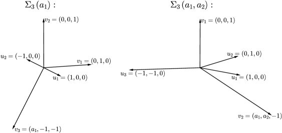
Figure 1. Fans with five generating rays that correspond to smooth projective toric varieties of complex dimension three

Lemma 5.3.

For the smooth projective toric varieties classified by Kleinschmidt in complex dimension three, we have $c_{1}^{3}\left[X_{3}\left(a_{1},a_{2}\right)\right]=54$ and $c_{1}^{3}\left[X_{3}\left(a_{1}\right)\right]=2a_{1}^{2}+54$.

Proof.

Theorem 2.10 can be used to compute the cohomology rings

$$H^{*}\left(X_{3}\left(a_{1},a_{2}\right)\right)\cong\mathbb{Z}\left[u_{3},v_{2}\right]/\left(u_{3}^{3}-\left(a_{1}+a_{2}\right)u_{3}^{2}v_{2},v_{2}^{2}\right)$$

and

$$H^{*}\left(X_{3}\left(a_{1}\right)\right)\cong\mathbb{Z}\left[u_{2},v_{3}\right]/\left(u_{2}^{2}-a_{1}u_{2}v_{3},v_{3}^{3}\right).$$

Theorem 2.12 can then be used to compute the cohomology classes $c_{1}\left(X_{3}\left(a_{1},a_{2}\right)\right)^{3}$ and $c_{1}\left(X_{3}\left(a_{1}\right)\right)^{3}$ in these cohomology rings. Using Proposition 2.11 to evaluate these cohomology classes on the fundamental class of the appropriate variety gives the result. ∎

Part 3 of Theorem 5.1 is a consequence of this lemma and Kleinschmidt’s classification result.

Since any cobordism class $\left[M\right]\in\Omega_{6}^{U}$ must have an even value for $c_{3}\left[M\right]$ by Proposition 5.2, part 4 of Theorem 5.1 states that for sufficiently large values of $c_{3}\left[M\right]$, the only obstructions to a cobordism class containing a smooth projective toric variety arise from the $g$-vector relations. To prove this, a smooth projective toric variety will be constructed with each possible combination of Chern numbers. As a start, we will find a smooth projective toric variety for each cobordism class with $c_{1}c_{2}\left[M\right]=24$ and $c_{3}\left[M\right]=8$.

Lemma 5.4.

Choose $a\in\mathbb{Z}$, and let $\Sigma\left(a\right)$ be the fan shown in Figure 2. The maximal cones in $\Sigma\left(a\right)$ are all cones spanned by one of the $u_{k}$, one of the $v_{k}$, and one of the $w_{k}$. The corresponding smooth projective toric variety $X\left(a\right)$ satisfies $c_{1}c_{2}\left[X\left(a\right)\right]=24$, $c_{3}\left[X\left(a\right)\right]=8$, and $c_{1}^{3}\left[X\left(a\right)\right]=48+2a$.

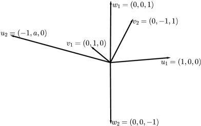
Figure 2. The fan $\Sigma\left(a\right)$

Proof.

It is straight-forward to verify that $X\left(a\right)$ is a smooth projective toric variety. More specifically, $X\left(a\right)$ is a $\mathbb{C}P^{1}$-bundle over the Hirzebruch surface $\mathcal{H}_{a}$. The polytope associated to $X\left(a\right)$ is combinatorially equivalent to a cube. Thus the $g$-vector of this polytope is $\left(1,2\right)$. Then $c_{1}c_{2}\left[X\left(a\right)\right]=24$, and $c_{3}\left[X\left(a\right)\right]=8$ by (5.1).

The structure of the fan $\Sigma\left(a\right)$ can be used to compute the integer cohomology ring $H^{*}\left(X\left(a\right)\right)\cong\mathbb{Z}\left[u_{2},v_{2},w_{2}\right]/\left(u_{2}^{2},v_{2}^{2}-au_{2}v_{2},w_{2}^{2}-v_{2}w_{2}\right)$. Computing $c_{1}\left(X\left(a\right)\right)^{3}$ in this cohomology ring produces $c_{1}\left(X\left(a\right)\right)^{3}=\left(48+2a\right)u_{2}v_{2}w_{2}$. Since $\mbox{pos}\left(u_{2},v_{2},w_{2}\right)$ is a maximal cone in $\Sigma\left(a\right)$, this means that $c_{1}^{3}\left[X\left(a\right)\right]=48+2a$ according to Proposition 2.11. ∎

Since $c_{1}^{3}\left[M\right]$ must be even by Proposition 5.2, this lemma tells us that any cobordism class satisfying $c_{1}c_{2}\left[M\right]=24$ and $c_{3}\left[M\right]=8$ can be represented by a smooth projective toric variety by choosing $X\left(a\right)$ with an appropriate value for $a$.

Next we consider all cobordism classes with $c_{3}\left[M\right]\geq 8$.

Lemma 5.5.

Let $X_{1}$ be a smooth projective toric variety with associated fan $\Sigma_{X_{1}}$ in $\mathbb{R}^{3}$. Suppose $\Sigma_{X_{2}}$ is obtained through a regular star subdivision of a maximal cone in $\Sigma_{X_{1}}$. That is, $X_{2}$ is an equivariant blow-up of $X_{1}$ at a torus-fixed point. Then the change in complex cobordism is given by $c_{2}\left[X_{2}\right]=c_{2}\left[X_{1}\right]$, $c_{3}\left[X_{2}\right]=c_{3}\left[X_{1}\right]+2$, and $c_{1}^{3}\left[X_{2}\right]=c_{1}^{3}\left[X_{1}\right]-8$.

Proof.

By Proposition 2.25, the change in cobordism only depends on the closed star of the cone that is being subdivided. By applying an appropriate unimodular transformation, we can assume without loss of generality that the cone being subdivided is $\mbox{pos}\left(e_{1},e_{2},e_{3}\right)$, where $e_{k}$ is the $k^{\mbox{th}}$ standard basis vector. The closed star of this maximal cone is $\mbox{pos}\left(e_{1},e_{2},e_{3}\right)$ itself, so the change in cobordism during an equivariant blow-up at a torus-fixed point is the same for any toric variety. This means that it suffices to compute the change in Chern numbers for just one specific example.

For simplicity, choose $X_{1}=\mathbb{C}P^{3}$, so $c_{1}c_{2}\left[X_{1}\right]=24$, $c_{3}\left[X_{1}\right]=4$, and $c_{1}^{3}\left[X_{1}\right]=64$. Let $X_{2}$ be the smooth projective toric variety associated to the fan obtained by subdividing the cone $\mbox{pos}\left(e_{1},e_{2},e_{3}\right)$ in the fan corresponding to $X_{1}$. Using Theorems 2.10, 2.12, and Proposition 2.11, we can compute $c_{1}c_{2}\left[X_{2}\right]=24=c_{1}c_{2}\left[X_{1}\right]$, $c_{3}\left[X_{2}\right]=6=c_{3}\left[X_{1}\right]+2$, and $c_{1}^{3}\left[X_{2}\right]=56=c_{1}^{3}\left[X_{1}\right]-8$. This proves the lemma. ∎

Now part 4 of Theorem 5.1 can be proven by using these blow-ups.

Proof of Theorem 5.1 part 4.

By Lemma 5.4, any cobordism class satisfying $c_{1}c_{2}\left[M\right]=24$ and $c_{3}\left[M\right]=8$ can be represented by a smooth projective toric variety. According to Lemma 5.5, each equivariant blow-up at a torus-fixed point increases the value of $c_{3}\left[M\right]$ by two and decreases the value of $c_{1}^{3}\left[M\right]$ by eight. Since these Chern numbers must always be even by Proposition 5.2, applying sufficiently many blow-ups to the smooth projective toric varieties $X\left(a\right)$ produces smooth projective toric varieties in every complex cobordism class with $c_{1}c_{2}\left[M\right]=24$ and $c_{3}\left[M\right]\in\left\{8,10,12,\ldots\right\}$. ∎

6. Smooth Projective Toric Varieties in $\Omega_{8}^{U}$

The techniques used to answer Question 1.2 in $\Omega_{6}^{U}$ can be applied to $\Omega_{8}^{U}$ as well. Unfortunately, the outcome in this dimension is significantly more complicated. In this case, there are $\left|\pi\left(4\right)\right|=5$ Chern numbers that determine a cobordism class, but only $\left\lfloor\frac{4+2}{2}\right\rfloor=3$ of these are determined by $g$-vectors in the case of smooth projective toric varieties. Because of a less complete understanding of smooth 4-polytopes compared to smooth polyhedra, only partial results can be obtained by extending the techniques that were used in $\Omega_{6}^{U}$.

First, we will find a convenient description for the restrictions from Theorem 3.5 in this dimension. These relations are $1=T_{4}^{0}\left[M\right]$, $-\left(1+g_{1}\right)=T_{4}^{1}\left[M\right]$, and $1+g_{1}+g_{2}=T_{4}^{2}\left[M\right]$, if $\left[M\right]\in\Omega_{8}^{U}$ contains a smooth projective toric variety. The definition of $T_{4}^{p}\left[M\right]$ and some computation can be used to write these relations in a more useful format (cf. [30, Section 4.4] and [20]). Combining the relations with the $g$-theorem (Theorem 2.16) gives the following result, which is just Theorem 3.6 applied to $n=4$.

Theorem 6.1.

Let $\left[M\right]\in\Omega_{8}^{U}$. If $\left[M\right]$ does not satisfy the equations

$$c_{4}\left[M\right] =5+3g_{1}+g_{2}$$

$$c_{1}c_{3}\left[M\right] =50+6g_{1}-2g_{2}$$

$$c_{1}^{4}\left[M\right] =4c_{1}^{2}c_{2}\left[M\right]+3c_{2}^{2}\left[M\right]+3g_{1}-3g_{2}-675$$

for some $g$-vector $\left(1,g_{1},g_{2}\right)$ such that $0\leq g_{1}$ and $0\leq g_{2}\leq\frac{1}{2}g_{1}\left(g_{1}+1\right)$, then $\left[M\right]$ does not contain a smooth projective toric variety.

As expected, the $g$-vector places obstructions on three of the Chern numbers, and the remaining two Chern numbers $c_{1}^{2}c_{2}\left[M\right]$ and $c_{2}^{2}\left[M\right]$ are independent of the $g$-vector. Note that there could be further restrictions on the $g$-vector beyond what the $g$-theorem provides for simple polytopes since our polytopes are also required to be smooth.

6.1. K-theory Chern numbers and $\Omega_{8}^{U}$

Before describing the cobordism classes that contain smooth projective toric varieties, it is again essential to know exactly which combinations of Chern numbers correspond to complex cobordism classes in $\Omega_{8}^{U}$. In this dimension, complex cobordism is determined by $\left|\pi\left(4\right)\right|=5$ Chern numbers. That means there are twelve K-theory Chern numbers arising from the partitions of nonnegative integers less than five. According to the Hattori-Stong Theorem (Theorem 2.4), each of these gives a divisibility relation on the Chern numbers of a complex cobordism class in $\Omega_{8}^{U}$.

For example, consider the empty partition. In this case, $s_{\varnothing}\left(\right)=1$, so the corresponding K-theory Chern number is

$$\kappa_{\varnothing}\left[M\right] =\mbox{Td}\left[M\right]=\frac{1}{720}\left(-c_{1}^{4}\left[M\right]+4c_{1}^{2}c_{2}\left[M\right]+3c_{2}^{2}\left[M\right]+c_{1}c_{3}\left[M\right]-c_{4}\left[M\right]\right)$$

(cf. [16, Section 1.7]). This gives the divisibility relation

$$-c_{1}^{4}\left[M\right]+4c_{1}^{2}c_{2}\left[M\right]+3c_{2}^{2}\left[M\right]+c_{1}c_{3}\left[M\right]-c_{4}\left[M\right]\equiv 0\mod 720$$

for Chern numbers in $\Omega_{8}^{U}$.

A similar process can be used to find the divisibility relations resulting from the remaining partitions (see [30, Section 4.4] for details). These are given in Table 1.The remaining five partitions not listed in the table are partitions of the complex dimension four itself. For these partitions, $\kappa_{\omega}\left[M\right]$ is already an integer combination of Chern numbers, so these do not impose any additional divisibility relations. The relations in Table 1 can be combined to give a characterization of all combinations of Chern numbers in $\Omega_{8}^{U}$.

Partition	Divisibility Relation
$\varnothing$	$-c_{1}^{4}\left[M\right]+4c_{1}^{2}c_{2}\left[M\right]+3c_{2}^{2}\left[M\right]+c_{1}c_{3}\left[M\right]-c_{4}\left[M\right]\equiv 0\mod 720$
$\left\{1\right\}$	$2c_{1}^{4}\left[M\right]-5c_{1}^{2}c_{2}\left[M\right]+5c_{1}c_{3}\left[M\right]-2c_{4}\left[M\right]\equiv 0\mod 12$
$\left\{1,1\right\}$	$6c_{1}^{2}c_{2}\left[M\right]-17c_{1}c_{3}\left[M\right]+14c_{4}\left[M\right]\equiv 0\mod 12$
$\left\{2\right\}$	$14c_{1}^{4}\left[M\right]-47c_{1}^{2}c_{2}\left[M\right]+12c_{2}^{2}\left[M\right]+46c_{1}c_{3}\left[M\right]-28c_{4}\left[M\right]\equiv 0\mod 12$
$\left\{1,1,1\right\}$	none (since $\kappa_{\left\{1,1,1\right\}}\left[M\right]=c_{1}c_{3}\left[M\right]-2c_{4}\left[M\right]\in\mathbb{Z}$)
$\left\{1,2\right\}$	$3c_{1}^{2}c_{2}\left[M\right]-2c_{2}^{2}\left[M\right]-9c_{1}c_{3}\left[M\right]+12c_{4}\left[M\right]\equiv 0\mod 2$
$\left\{3\right\}$	$4c_{1}^{4}\left[M\right]-15c_{1}^{2}c_{2}\left[M\right]+6c_{2}^{2}\left[M\right]+15c_{1}c_{3}\left[M\right]-12c_{4}\left[M\right]\equiv 0\mod 2$

Table 1. Divisibility relations for Chern numbers in $\Omega_{8}^{U}$

Proposition 6.2.

A complex cobordism class $\left[M\right]\in\Omega_{8}^{U}$ can have Chern numbers $c_{1}^{4}\left[M\right]$, $c_{1}^{2}c_{2}\left[M\right]$, $c_{2}^{2}\left[M\right]$, $c_{1}c_{3}\left[M\right]$, and $c_{4}\left[M\right]$ if and only if the following divisibility relations hold.

$$-c_{1}^{4}\left[M\right]+4c_{1}^{2}c_{2}\left[M\right]+3c_{2}^{2}\left[M\right]+c_{1}c_{3}\left[M\right]-c_{4}\left[M\right] \equiv 0\mod 720$$

$$6c_{1}^{2}c_{2}\left[M\right]-5c_{1}c_{3}\left[M\right]+2c_{4}\left[M\right] \equiv 0\mod 12$$

$$c_{1}^{2}c_{2}\left[M\right]+c_{1}c_{3}\left[M\right] \equiv 0\mod 2$$

$$2c_{1}^{4}\left[M\right]-5c_{1}^{2}c_{2}\left[M\right]+5c_{1}c_{3}\left[M\right]-2c_{4}\left[M\right] \equiv 0\mod 12$$

$$2c_{1}^{4}\left[M\right]+c_{1}^{2}c_{2}\left[M\right]-2c_{1}c_{3}\left[M\right]-4c_{4}\left[M\right] \equiv 0\mod 12$$

6.2. Smooth projective toric varieties representing $\Omega_{8}^{U}$

The description of possible Chern numbers of cobordism classes is clearly much more complicated in dimension eight compared to dimension six. Fortunately, to address Question 1.2, we are only concerned with cobordism classes which contain smooth projective toric varieties. These classes must also satisfy the conditions given in Theorem 6.1. Substituting these conditions into the first relation of Proposition 6.2 shows that it is always satisfied for cobordism classes which contain smooth projective toric varieties. (This is equivalent to the fact that the Todd genus must be one.) The second relation in Proposition 6.2 simplifies to $c_{1}^{2}c_{2}\left[M\right]\equiv 0\mod 2$. Since $c_{1}c_{3}\left[M\right]=50+6g_{1}-2g_{2}$ is always even, the third relation in Proposition 6.2 is automatically satisfied for any complex cobordism class containing a smooth projective toric variety. Theorem 6.1 can be used to rewrite the remaining relations of Proposition 6.2 as $c_{1}^{2}c_{2}\left[M\right]+2c_{2}^{2}\left[M\right]+c_{1}c_{3}\left[M\right]\equiv 0\mod 4$. Combining these simplified relations with the $g$-theorem for simple polytopes gives a more convenient way of writing the necessary conditions for a cobordism class in $\Omega_{8}^{U}$ to contain a smooth projective toric variety.

Theorem 6.3.

Let $\left[M\right]\in\Omega_{8}^{U}$. If $\left[M\right]$ does not satisfy all of the following conditions for some $g$-vector $\left(1,g_{1},g_{2}\right)$, then $\left[M\right]$ does not contain a smooth projective toric variety.

$$0 \leq g_{1}$$

$$0 \leq g_{2}\leq\frac{1}{2}g_{1}\left(g_{1}+1\right)$$

$$c_{4}\left[M\right] =5+3g_{1}+g_{2}$$

$$c_{1}c_{3}\left[M\right] =50+6g_{1}-2g_{2}$$

$$c_{1}^{4}\left[M\right] =4c_{1}^{2}c_{2}\left[M\right]+3c_{2}^{2}\left[M\right]+3g_{1}-3g_{2}-675$$

$$c_{1}^{2}c_{2}\left[M\right] \equiv 0\mod 2$$

$$c_{1}^{2}c_{2}\left[M\right]+2c_{2}^{2}\left[M\right]+c_{1}c_{3}\left[M\right] \equiv 0\mod 4$$

These relations have three different sources. The first two come from the $g$-theorem. The next three are obstructions arising from the relation between the $g$-vector and Chern numbers (see (3.3)). The last two arise from the Hattori-Stong Theorem, and they must be satisfied for any cobordism class in $\Omega_{8}^{U}$.

As in $\Omega_{6}^{U}$, these conditions on cobordism classes in $\Omega_{8}^{U}$ are not sufficient conditions for containing smooth projective toric varieties, and a detailed study must be made to describe smooth projective toric varieties in a given cobordism class. Unfortunately, much less is understood about four-dimensional smooth polytopes compared to smooth polyhedra, so only partial results can be obtained in this dimension. First, we will focus on smooth 4-polytopes with $g_{1}\leq 2$, as these have been completely classified.

Theorem 6.4.

Suppose $\left[M\right]\in\Omega_{8}^{U}$ satisfies the conditions in Theorem 6.3, and suppose $g_{1}=0$. Then $\left[M\right]$ contains a smooth projective toric variety if and only if $\left[M\right]=\left[\mathbb{C}P^{4}\right]$.

Proof.

This follows from the fact that the only smooth 4-polytope with $g_{1}=0$ is the 4-simplex, whose associated smooth projective toric variety is $\mathbb{C}P^{4}$. ∎

This shows that the conditions of Theorem 6.3 are not sufficient. For example, let $\left(1,g_{1},g_{2}\right)=\left(1,0,0\right)$ and $\left(c_{1}^{4}\left[M\right],c_{1}^{2}c_{2}\left[M\right],c_{2}^{2}\left[M\right],c_{1}c_{3}\left[M\right],c_{4}\left[M\right]\right)=\left(-672,0,1,50,5\right)$. This represents a valid cobordism class in $\Omega_{8}^{U}$ that satisfies all of the conditions of 6.3. However, $c_{1}^{4}\left[M\right]\neq 625=c_{1}^{4}\left[\mathbb{C}P^{4}\right]$, so $\left[M\right]\neq\left[\mathbb{C}P^{4}\right]$. Thus $\left[M\right]$ does not contain a smooth projective toric variety.

Smooth 4-polytopes with $g_{1}=1$ have also been completely classified. These are the smooth 4-polytopes having exactly six facets, two more than the ambient dimension. The corresponding normal fans to these polytopes were classified by Kleinschmidt [19], and they are just a generalization of the three-dimensional fans with five facets shown in Figure 1. More specifically, choose an integer $r\in\left\{1,2,3\right\}$ and a set of weakly increasing integers $0\leq a_{1}\leq\ldots\leq a_{r}$. Define $U=\left\{u_{1},\ldots,u_{r+1}\right\}$, where $u_{k}=e_{k}$ is the standard basis vector for $k=1,\ldots,r$, and set $u_{r+1}=\left(-1,\stackrel{{\scriptstyle\left(r\right)}}{{\ldots}},-1,0,\ldots,0\right)$. Also define $V=\left\{v_{1},\ldots,v_{n-r+1}\right\}$, where $v_{k}=e_{k+r}$ for $k=1,\ldots,n-r$, and set $v_{n-r+1}=\left(a_{1},\ldots,a_{r},-1,\ldots,-1\right)$. Let $\Sigma_{4}\left(a_{1},\ldots,a_{r}\right)$ denote the fan whose generating rays are the six rays in $U\cup V$ and whose maximal cones are obtained by taking the span of all but one vector from $U$ and all but one vector from $V$. Kleinschmidt proved that the associated toric varieties $X_{4}\left(a_{1},\ldots,a_{r}\right)$ are smooth and projective, and he demonstrated that every smooth toric variety in this dimension whose associated fan has six rays is isomorphic to one of these varieties [19]. Thus if a smooth 4-polytope satisfies $g_{1}=1$, then its associated smooth projective toric variety is isomorphic to one of the $X_{4}\left(a_{1},\ldots,a_{r}\right)$.

Theorem 6.5.

Suppose $\left[M\right]\in\Omega_{8}^{U}$ satisfies the conditions in Theorem 6.3, and suppose $g_{1}=1$. Then $\left[M\right]$ contains a smooth projective toric variety if and only if

$$\left[M\right]\in\left\{\left[X_{4}\left(a_{1}\right)\right],\left[X_{4}\left(a_{1},a_{2}\right)\right],\left[X_{4}\left(a_{1},a_{2},a_{3}\right)\right]\right\}$$

for some integers $0\leq a_{1}\leq a_{2}\leq a_{3}$.

Remark 6.6.

Batyrev gave a similar classification for smooth projective toric varieties whose polytopes have three more facets than the ambient dimension [2]. In dimension four, a polytope has seven facets if and only if $g_{1}=2$. This means that a cobordism class $\left[M\right]\in\Omega_{8}^{U}$ that satisfies the conditions of Theorem 6.3 with $g_{1}=2$ contains a smooth projective toric variety if and only if it equals the cobordism class of one of the varieties classified by Batyrev. Specific conditions on the Chern numbers can be listed for these varieties by computing the Chern numbers for each possible variety classified by Batyrev. However, these conditions are quite complicated, and they do not reveal any surprising structure. One thing that is clear from these computations is that once again, the necessary conditions from Theorem 6.3 are not the only obstructions to a cobordism class containing a smooth projective toric variety.

For $g_{1}\in\left\{0,1,2\right\}$, the description of which cobordism classes contain smooth projective toric varieties is quite complicated, and it depends on much more than the $g$-vector. However, as this $g$-vector grows larger in some sense, there is more freedom on the geometry of the corresponding smooth 4-polytopes. In particular, for a certain infinite set of $g$-vectors in this dimension, the $g$-vector does provide the only obstructions to a cobordism class containing a smooth projective toric variety.

Theorem 6.7.

Suppose $\left[M\right]\in\Omega_{8}^{U}$ satisfies the conditions of Theorem 6.3 for some $g$-vector such that $2\leq g_{2}\leq g_{1}-1$. Then $\left[M\right]$ is represented by a smooth projective toric variety.

Proof.

This theorem will be proven using a technique similar to that of part 4 of Theorem 5.1. First, an explicit construction will be used to show that the conditions of Theorem 6.3 are sufficient for the $g$-vector $\left(1,3,2\right)$. Next, a sequence of blow-ups will be used to obtain smooth projective toric varieties corresponding to the other possible $g$-vectors.

First, we must describe a collection of smooth projective toric varieties to account for all possible cobordism classes corresponding to the $g$-vector $\left(1,3,2\right)$. These can most easily be described in terms of the corresponding fans. Choose two integers $a$ and $b$, and consider the fan $\Delta\left(a,b\right)$ whose generating rays are depicted in Figure 3. This fan is the join of two fans. That is, a maximal cone in $\Delta\left(a,b\right)$ is obtained by taking the combined span of a maximal cone from each of the smaller fans. To construct the fan on the left, start with the fan with generating rays $u_{1},\ u_{2},\ u_{3},$ and $u_{4}$ that corresponds to the toric variety $\mathbb{C}P^{3}$. Take the regular star subdivision of the cone $\mbox{pos}\left(u_{3},u_{4}\right)$, and let $x=\left(-1,-1,0,0\right)$ denote the additional vector. Finally, take the regular star subdivision of $\mbox{pos}\left(u_{1},u_{3},x\right)$, and let $y=\left(0,-1,1,0\right)$ denote the new generating ray. The join of this fan and the fan on the right is complete and regular, so $\Delta\left(a,b\right)$ corresponds to a smooth projective toric variety $Y\left(a,b\right)$ of complex dimension four.

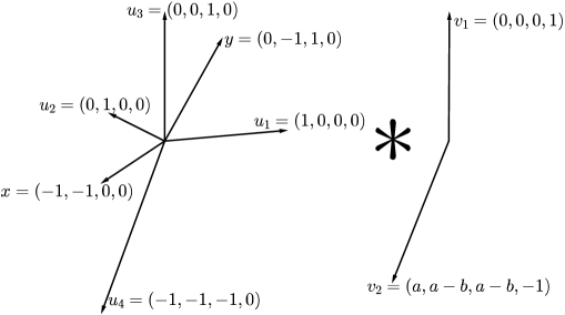
Figure 3. The fan $\Delta\left(a,b\right)$

The simplicial structure of $\Delta\left(a,b\right)$ can be determined by tracking the maximal cones through each subdivision. In particular, the Stanley-Reisner ideal for this fan is

$$\left(u_{2}y,u_{3}u_{4},u_{4}y,v_{1}v_{2},u_{1}u_{2}x,u_{1}u_{3}x\right).$$

This along with the coordinates of the generating rays can be used to compute the cohomology of $Y\left(a,b\right)$ using Theorem 2.10. Theorem 2.12 can then be used to obtain the values for the Chern numbers

$$c_{1}^{2}c_{2}\left[Y\left(a,b\right)\right]=188-6a+4b$$

and

$$c_{2}^{2}\left[Y\left(a,b\right)\right]=96-a.$$

We must show that all possible combinations of Chern numbers are obtained by the toric varieties $Y\left(a,b\right)$. Since we are requiring $g=\left(1,3,2\right)$, we have $c_{1}c_{3}\left[M\right]=64$ for any cobordism class $\left[M\right]\in\Omega_{8}^{U}$ that possibly contains a smooth projective toric variety, according to Theorem 6.3. It therefore suffices to show that every combination of values for $c_{1}^{2}c_{2}\left[M\right]$ and $c_{2}^{2}\left[M\right]$ such that $c_{1}^{2}c_{2}\left[M\right]$ is even and $c_{1}^{2}c_{2}\left[M\right]+2c_{2}^{2}\left[M\right]\equiv 0\mod 4$ are obtained by the varieties $Y\left(a,b\right)$ (see Theorem 6.3). Since $c_{2}^{2}\left[Y\left(a,b\right)\right]$ depends on $a$ alone, we can choose $b$ appropriately to achieve this.

Now that all cobordism classes corresponding to the $g$-vector $\left(1,3,2\right)$ have been represented by smooth projective toric varieties, certain blow-ups can be used to obtain smooth projective toric varieties for other $g$-vectors. On the level of fans, consider star subdivisions of maximal four-dimensional cones and also star divisions of three-dimensional cones. The change in $g$-vector of the corresponding polytope during these star divisions is described in Propositions 2.23 and 2.24. In this dimension, if a polytope has $g$-vector $\left(1,g_{1},g_{2}\right)$, then taking a star division of a maximal cone of its normal fan produces a fan that is normal to a polytope with $g$-vector $\left(1,g_{1}+1,g_{2}\right)$. On the other hand, taking a star division of a three-dimensional cone changes the $g$-vector to $\left(1,g_{1}+1,g_{2}+1\right)$. This means that any $g$-vector that satisfies $2\leq g_{2}\leq g_{1}-1$ can be obtained by a smooth polytope through a sequence of truncations applied to a smooth polytope with $g$-vector $\left(1,3,2\right)$.

Consider an arbitrary $g$-vector $\left(1,g_{1},g_{2}\right)$ such that $2\leq g_{2}\leq g_{1}-1$. Starting with the fans $\Delta\left(a,b\right)$, fix a sequence of regular star subdivisions that will produce a fan normal to a polytope with $g$-vector $\left(1,g_{1},g_{2}\right)$. Choose these star subdivisions so that any cone in the closed star of the ray $v_{2}$ is never subdivided. By Proposition 2.25, the change in cobordism during this sequence of subdivisions does not depend on the values of $a$ and $b$. In other words, the values of $c_{1}^{2}c_{2}\left[M\right]$ and $c_{2}^{2}\left[M\right]$ change by the same constants during this sequence of subdivisions regardless of the values of $a$ and $b$ for the initial toric variety $Y\left(a,b\right)$. Since all possible cobordism classes are represented by the smooth projective toric varieties $Y\left(a,b\right)$ for $g$-vector $\left(1,3,2\right)$, applying this sequence of subdivisions allows us to obtain a smooth projective toric variety in every cobordism class with $g$-vector $\left(1,g_{1},g_{2}\right)$. ∎

The $g$-vectors for which the conditions in Theorem 6.3 are also sufficient are displayed in Figure 4. The lattice points correspond to all possible $g$-vectors for simple 4-polytopes (using the $g$-theorem), and the shaded area gives the $g$-vectors described in Theorem 6.7.

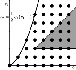
Figure 4. The $g$-vectors that satisfy the conditions of Theorem 6.7

There are still many $g$-vectors for which the answer to Question 1.2 is open in $\Omega_{8}^{U}$. A more complete classification of smooth 4-polytopes could help to determine what happens for the remaining $g$-vectors. Unfortunately, very little is known regarding this classification. It is not even known which $g$-vectors correspond to smooth polytopes. The $g$-theorem describes all $g$-vectors of simple polytopes, and this gives necessary conditions for the $g$-vectors of smooth polytopes since smooth polytopes are also simple. However, not every such $g$-vector actually corresponds to a smooth polytope. For example, consider the smooth 4-polytopes with $g_{1}=2$ (i.e. with seven facets) that were classified by Batyrev [2]. It is easy to compute the $g$-vector of each of these smooth polytopes. The only possible values for $g_{2}$ are $0,\ 1,\$and $2$. This means that although there is a simple 4-polytope with $g$-vector $\left(1,2,3\right)$, there is no smooth 4-polytope with this $g$-vector.

Proposition 6.8.

Suppose $\left[M\right]\in\Omega_{8}^{U}$ satisfies the conditions of Theorem 6.3 with $g$-vector $\left(1,2,3\right)$. Then there is no smooth projective toric variety that can be chosen to represent $\left[M\right]$.

A refinement of the $g$-theorem for smooth 4-polytopes could improve Theorem 6.3 by providing more stringent necessity conditions.

7. Closing Remarks

It seems reasonable to expect that Hirzebruch’s Question regarding which complex cobordism classes contain connected smooth algebraic varieties would be greatly simplified by only considering smooth projective toric varieties. Even when this is done, the results are quite complicated. A complete answer to Question 1.2 has only been given up to complex dimension three. The same techniques that produce partial results in complex dimension four quickly become too cumbersome as dimension increases further. In an arbitrary dimension $n$, the $g$-theorem for simple polytopes and the combinatorial obstructions of Theorem 3.5 provide obstructions to $\left\lfloor\frac{n+2}{2}\right\rfloor$-many of the Chern numbers of cobordism classes containing smooth projective toric varieties. Unfortunately, the total number $\left|\pi\left(n\right)\right|$ of Chern numbers needed to describe complex cobordism classes in $\Omega_{2n}^{U}$ increases much more quickly than this number of obstructions. As dimension increases, the combinatorial structure of smooth projective toric varieties seems to have an ever diminishing influence on complex cobordism.

It is also impractical to explicitly describe all possible combinations of Chern numbers in higher dimensions using the Hattori-Stong Theorem as it was done up to complex dimension four. Perhaps studying $g$-vectors and Chern numbers may not be the best way to approach Question 1.2. It may be worthwhile to search for other invariants of polytopes or cobordism classes that give a more complete answer.

There are also several ways in which the partial results for Question 1.2 could possibly be refined or extended. In both complex dimensions three and four, there is a collection of $g$-vectors for which the only obstructions to a cobordism class containing a smooth projective toric variety are the combinatorial obstructions from Theorem 3.5. These $g$-vectors allow enough geometric freedom to construct a large collection of smooth polytopes which correspond to smooth projective toric varieties in any potential cobordism class. For higher dimensions, it would be interesting to see if a similar asymptotic result holds. Does the amount of geometric freedom for certain $g$-vectors increase quickly enough compared to the rapid increase in how many Chern numbers are independent of the $g$-vector?

Question 7.1.

Given an arbitrary complex dimension $n$, is there a collection of $g$-vectors such that the only obstructions to a cobordism class $\left[M\right]\in\Omega_{2n}^{U}$ containing a smooth projective toric variety are the combinatorial obstructions given in Theorem 3.5?

Since there is a bijective correspondence between smooth projective toric varieties and smooth polytopes, another way of approaching Question 1.2 is to determine a more complete classification of smooth polytopes. For example, all smooth $n$-dimensional polytopes with $g_{1}\in\left\{0,1,2\right\}$ have been completely classified. The only polytope with $g_{1}=0$ is the $n$-simplex, and those with $g_{1}=1$ and $g_{1}=2$ were classified by Kleinschmidt [19] and Batyrev [2], respectively. Thus it is known which cobordism classes that satisfy Theorem 3.5 with $g_{1}\in\left\{0,1,2\right\}$ contain smooth projective toric varieties. A more complete classification of smooth polytopes could lead to more results of this type.

As a start to this classification, it would be useful to know all $g$-vectors that correspond to smooth polytopes. Since all smooth polytopes are simple, the restrictions in the $g$-theorem are necessary but not sufficient.

Question 7.2.

Which vectors can be obtained as $g$-vectors for smooth polytopes?

Answering this question would immediately allow us to improve Theorems 3.5 and 3.6 with more stringent conditions.

References

- [1] M. F. Atiyah. Immersions and embeddings of manifolds. Topology, 1:125–132, 1961.
- [2] Victor V. Batyrev. On the classification of smooth projective toric varieties. Tohoku Mathematical Journal, 43:569–585, 1991.
- [3] Louis J. Billera and Carl W. Lee. Sufficiency of McMullen’s conditions for f-vectors of simplicial polytopes. Bulletin of the American Mathematical Society, 2(1):181–185, 1980.
- [4] V. M. Buchstaber and N. Ray. Toric manifolds and complex cobordisms. Russian Mathematical Surveys, 53(2):371–373, 1998.
- [5] Victor M. Buchstaber and Taras E. Panov. Torus Actions and Their Applications in Topology and Combinatorics, volume 24 of University Lecture Series. American Mathematical Society, Providence, RI, 2002.
- [6] Victor M Buchstaber and Nigel Ray. Tangential structures on toric manifolds, and connected sums of polytopes. International Mathematical Research Notices, 4:193–219, 2001.
- [7] P. E. Conner and E. E. Floyd. The Relation of Cobordism to K-Theories. Number 28 in Lecture Notes in Mathematics. Springer-Verlag, 1966.
- [8] David A. Cox, John B. Little, and Henry K. Schenck. Toric Varieties, volume 124 of Graduate Studies in Mathematics. American Mathematical Society, 2011.
- [9] V. I. Danilov. The geometry of toric varieties. Russian Mathematical Surveys, 33(2):97–154, 1978.
- [10] Günter Ewald. Combinatorial Convexity and Algebraic Geometry. Springer, 1996.
- [11] William Fulton. Introduction to Toric Varieties. Princeton University Press, 1993.
- [12] Phillip Griffiths and Joseph Harris. Principles of Algebraic Geometry. Wiley, New York, 1978.
- [13] A. Hattori. Integral characteristic numbers for weakly almost complex manifolds. Topology, 5:259–280, 1966.
- [14] Akio Hattori and Mikiya Masuda. Theory of multi-fans. Osaka Journal of Mathematics, 40(1):1–68, 2003.
- [15] F. Hirzebruch. Komplexe Mannigfaltigkeiten. In Proceedings of the International Congress of Mathematicians, pages 119–136, 1958.
- [16] F. Hirzebruch. Topological Methods in Algebraic Geometry. Springer-Verlag, third edition, 1966.
- [17] Masa-Nori Ishida. Polyhedral Laurent series and Brion’s equalities. International Journal of Mathematics, 1(3):251–265, 1990.
- [18] J. Jurkiewicz. Torus embeddings, polyhedra, k*-actions and homology. Dissertationes Mathematicae, 236, 1985.
- [19] Peter Kleinschmidt. A classification of toric varieties with few generators. Aequationes Mathematicae, 35:254–266, 1988.
- [20] Anatoly S. Libgober and John W. Wood. Uniqueness of the complex structure on Kähler manifolds of certain homotopy types. Journal of Differential Geometry, 32:139–154, 1990.
- [21] K. H. Mayer. Relationen zwischen charakteristischen Zahlen. Number 111 in Lecture Notes in Mathematics. Springer Verlag, 1969.
- [22] J. Milnor. On the cobordism ring and a complex analogue. American Journal of Mathematics, 82(3):505–521, July 1960.
- [23] John W. Milnor and James D. Stasheff. Characteristic Classes. Number 76 in Annals of Mathematical Studies. Princeton University Press, 1974.
- [24] S. P. Novikov. Some problems in the topology of manifolds connected with the theory of Thom spaces. Doklady Akademii Nauk SSSR, 132(5):1031–1034, 1960.
- [25] Tadao Oda. Convex Bodies and Algebraic Geometry. Springer-Verlag, 1988.
- [26] Richard P. Stanley. The number of faces of a simplicial convex polytope. Advances in Mathematics, 35:236–238, 1980.
- [27] Robert E. Stong. Relations among characteristic numbers-i. Topology, 4:267–281, 1965.
- [28] Robert E. Stong. Notes on Cobordism Theory. Princeton University Press, 1968.
- [29] Yury Ustinovsky. Characteristic numbers of toric varieties from combinatorial point of view. Toric topology meeting, Osaka, Japan, November 2011.
- [30] Andrew Wilfong. Toric Varieties and Cobordism. PhD thesis, University of Kentucky, 2013.