On Rates of Convergence for Markov Chains under Random Time State Dependent Drift Criteria

Abstract

Many applications in networked control require intermittent access of a controller to a system, as in event-triggered systems or information constrained control applications. Motivated by such applications and extending previous work on Lyapunov-theoretic drift criteria, we establish both subgeometric and geometric rates of convergence for Markov chains under state dependent random time drift criteria. We quantify how the rate of ergodicity, nature of Lyapunov functions, their drift properties, and the distributions of stopping times are related. We finally study an application in networked control.

I Introduction and literature review

Stochastic stability of Markov chains has an almost complete theory, and forms a foundation for several other general techniques such as dynamic programming, linear programming approach to Markov Decision Processes [1], and Markov Chain Monte-Carlo (MCMC) [2]. One powerful approach to establish stochastic stability is through single-stage (Foster-Lyapunov) drift criteria [3]. The state-dependent criteria [4, 5, 6] relax the one-stage criteria to criteria involving time instances which are state-dependent but deterministic. Such criteria form the basis of the fluid-model (or ODE) approach to stability in stochastic networks and other general models [7], [8], [9], [10], [2]. Building on [3] and [4], [11] considered stability criteria based on a state-dependent random sampling of the Markov chain of the following form: It was assumed that there is positive real-valued function $V$ on the state space ${\mathbb{X}}$ of a discrete-time Markov chain $\{x_{t}\}_{t\geq 0}$, and an increasing sequence of stopping times $\{{\cal T}_{i}\}_{t\geq 0}$, with ${\cal T}_{0}=0$, such that for each $i$,

$$E[V(x_{{\cal T}_{i+1}})\mid{\cal F}_{{\cal T}_{i}}]\leq V(x_{{\cal T}_{i}})-\delta(x_{{\cal T}_{i}}),$$ (1)

where the function $\delta\colon{\mathbb{X}}\to\mathbb{R}$ is positive (bounded away from zero) outside of a “small set”, and ${\cal F}_{{\cal T}_{i}}$ denotes the filtration of “events up to time ${\cal T}_{i}$”. We will make this more precise later in the paper. Further relevant work include [12] and [6].

Motivation for studying such problems comes from networked control systems and communication systems: For many networked control scenarios, access to information or application of a control action in a system is limited to random event times. As examples for such settings, there has been significant research on stochastic stabilization of networked control systems and information theory; as in stabilization of adaptive quantizers studied in source coding [13], [14] and control theory [15], [16], [17], [18]. A specific example involving control over an erasure channel is given in [11], where non-zero stabilizing actions of a controller are applied to a system at certain event driven times and stochastic stability is shown using drift conditions and martingale techniques. For an extensive discussion, see [19]. The methods of random-time drift criteria can also be applied to models of networked control systems with delay-sensitive information transmission, for example, for studying the effects of randomness in the delay for transmission of sensor or controller signals (see, e.g., [20], [21], [22], [23]).

One other, increasingly prominent, area is event-triggered feedback control systems (see e.g. [24], [25], [26], [27], [28]) where the event instances constitute the stopping-times. The study of such systems is practically relevant since an event-based clock is usually more efficient than a time-triggered clock for control under information or actuation costs. The literature on such systems has primarily focused on the stabilization of such systems and we hope that the analysis in this paper will be useful for both stabilization and optimization of such systems: If the objective is to compute optimal solutions to an average cost optimization problem for an event triggered setup, a powerful approach is the discounted limit approach [29] [30]. This method typically requires geometric or sufficiently fast subgeometric convergence conditions to establish the existence of a solution to an average cost optimality equation or inequality [29]. The rate of convergence results in this paper will be useful in such contexts. Furthermore, rates of convergence to equilibrium in Markov chains are useful in bounding the distribution of transient events and the approximate computation of optimal costs under ergodicity properties. In addition, as documented extensively in the literature, Markov Chain Monte Carlo algorithms require a tedious analysis on rates of convergence bounds to obtain probabilistically guaranteed simulation times, see, e.g., [2], [31]. Furthermore, as has been discussed in [32] and [33], approximation methods for optimization of Markov Decision Processes benefit from the presence of sufficiently fast mixing/rates of convergence conditions.

In this paper, we extend recent works on random-time drift analysis [11] to obtain criteria for rates of convergence under subgeometric and geometric rate functions.

The rest of the paper is organized as follows. In Section II, we provide background information on Markov chains and rates of convergence to equilibrium. Section III contains the rate of convergence results under random-time state-dependent drift conditions. Section IV contains an example from networked control.

II Markov Chains, Stochastic Stability, and Rates of Convergence

In this section, we review some definitions and background material relating to Markov chains and their convergence to equilibrium.

II-A Preliminaries

We let $\{x_{t}\}_{t\geq 0}$ denote a discrete-time Markov chain with state space ${\mathbb{X}}$. The basic assumptions of [3] are adopted, see [34] for a more comprehensive introduction: It is assumed that ${\mathbb{X}}$ is a complete separable metric space; its Borel $\sigma$-field is denoted by ${\cal B}({\mathbb{X}})$. The transition probability is denoted by $P$, so that for any $x\in{\mathbb{X}}$, $A\in{{\cal B}(\mathbb{X})}$, the probability of moving in one step from the state $x$ to the set $A$ is given by $P(x_{t+1}\in A\mid x_{t}=x)=P(x,A)$. The $n$-step transitions are obtained via composition in the usual way, $P(x_{t+n}\in A\mid x_{t}=x)=P^{n}(x,A)$, for any $n\geq 1$. The transition law acts on measurable functions $f\colon{\mathbb{X}}\to\mathbb{R}$ and measures $\mu$ on ${{\cal B}(\mathbb{X})}$ via $Pf\,(x)\mathbin{:=}\int_{{\mathbb{X}}}P(x,dy)f(y),\quad x\in{\mathbb{X}},$ and $\mu P\,(A)\mathbin{:=}\int_{{\mathbb{X}}}\mu(dx)P(x,A)$, $A\in{\cal B}({\mathbb{X}})$. A probability measure $\pi$ on ${{\cal B}(\mathbb{X})}$ is called invariant if $\pi P=\pi$, i.e.,

$$\int\pi(dx)P(x,A)=\pi(A),\qquad A\in{{\cal B}(\mathbb{X})}.$$

For any initial probability measure $\nu$ on ${{\cal B}(\mathbb{X})}$ we can construct a stochastic process $\{x_{t}\}$ with transition law $P$ satisfying $x_{0}\sim\nu$. We let $P_{\nu}$ denote the resulting probability measure on the sample space $({\mathbb{X}},{\cal B}({\mathbb{X}}))^{\infty}$, with the usual convention for $\nu=\delta_{x}$ (where $\delta_{x}$ is the probability measure defined by $\delta_{x}(A)=1_{A}(x)$ for all Borel $A$ and $1_{E}(x)$ denotes the indicator function for the event $\{x\in E\}$) when the initial state is $x\in{\mathbb{X}}$, in which case we write $P_{x}$ for the resulting probability measure. Likewise, $E_{x}$ denotes the expectation operator when the initial condition is given by $x_{0}=x$.

When $\nu=\pi$ (the invariant measure), the resulting process is stationary. For a set $A\in{{\cal B}(\mathbb{X})}$ we denote,

$${\cal T}_{A}\mathbin{:=}\min\{t\geq 1:x_{t}\in A\}.$$ (2)

Definition II.1.

Let $\varphi$ denote a $\sigma$-finite measure on ${{\cal B}(\mathbb{X})}$. The Markov chain is called $\varphi$-irreducible if for any $x\in{\mathbb{X}}$, and any $B\in{{\cal B}(\mathbb{X})}$ satisfying $\varphi(B)>0$, we have $P_{x}\{{\cal T}_{B}<\infty\}>0$. A $\varphi$-irreducible Markov chain is aperiodic if for any $x\in{\mathbb{X}}$, and any $B\in{{\cal B}(\mathbb{X})}$ satisfying $\varphi(B)>0$, there exists $n_{0}=n_{0}(x,B)$ such that $P^{n}(x,B)>0\qquad\hbox{\it for all \ }n\geq n_{0}$. A $\varphi$-irreducible Markov chain is Harris recurrent if $P_{x}({\cal T}_{B}<\infty)=1$ for any $x\in{\mathbb{X}}$, and any $B\in{{\cal B}(\mathbb{X})}$ satisfying $\varphi(B)>0$. It is positive Harris recurrent if in addition there is an invariant probability measure $\pi$.

A maximal irreducibility measure is one with respect to which all other irreducibility measures are absolutely continuous. Define ${\cal B}^{+}({\mathbb{X}})=\left\{A\in{\cal B}({\mathbb{X}}):\psi(A)>0\right\}$, where $\psi$ is a maximal irreducibility measure. We refer to sets in ${\cal B}^{+}({\mathbb{X}})$ as reachable.

A set $A\in{\cal B}({\mathbb{X}})$ is full if $\psi(A^{c})=0$ for a maximal irreducibility measure $\psi$. A set $A\in{\cal B}({\mathbb{X}})$ is absorbing if $P(x,A)=1$ for all $x\in A$. In an irreducible Markov chain every absorbing set is full.

Definition II.2.

A set $\alpha\in{\cal B}^{+}({\mathbb{X}})$ is an atom if for all $x,y\in\alpha$ $P(x,\,\cdot\,)=P(y,\,\cdot\,)$.

The concept of an atom is extremely important as it gives us a fundamental unit, where all the points of a reachable set act together. This allows, through the cycle equation, an invariant probability measure $\pi(A)=E_{\alpha}\Big{[}\sum_{k=0}^{{\cal T}_{\alpha}-1}1_{A}(x_{k})\Big{]}/E_{\alpha}[{\cal T}_{\alpha}]$. When the state space is not countable, one typically needs to artificially construct such an atom, as we discuss further below.

Definition II.3.

A set $C\in{\cal B}^{+}({\mathbb{X}})$ is $(n_{0},\epsilon,\nu)$-small if

$$P^{n_{0}}(x,B)\geq\epsilon\nu(B)\quad\forall B\in{\cal B}({\mathbb{X}}),x\in C$$

where $n_{0}\geq 1$, $\epsilon\in(0,1)$, and $\nu$ is a positive measure on $({\mathbb{X}},{\cal B}({\mathbb{X}}))$.

An important fact is that small sets exist, see Theorem 5.2.1 of [3].

Fact II.1.

For an irreducible Markov chain, every set $A\in\mathcal{B^{+}({\mathbb{X}})}$ contains a small set in $\mathcal{B^{+}({\mathbb{X}})}$.

Definition II.4.

A set $C\in{\cal B}^{+}({\mathbb{X}})$ is called $\kappa$-petite if there is a positive measure $\kappa$ on ${\cal B}({\mathbb{X}})$ and a probability distribution $a$ on $\mathbb{Z}_{+}=\{0,1,2\ldots\}$ such that

$$\sum\limits_{n=0}^{\infty}a(n)P^{n}(x,B)\geq\kappa(B)\quad\text{for all }B\in{\cal B}({\mathbb{X}}),\;x\in C.$$ (3)

The convolution of two functions $f,g:\mathbb{Z}_{+}\rightarrow\mathbb{R}$, denoted by $f\ast g$, is defined as usual by $f\ast g(n)=\sum\limits_{k=0}^{n}f(k)g(n-k)$, for all $n\in\mathbb{Z}_{+}$. The next lemma follows from Lemma 5.5.2 of [3] and allows us to assume without loss of generality that for an irreducible Markov chain, if a set is $\kappa$-petite, then $\kappa$ can be replaced by maximal irreducibility measure (or equivalently $\kappa$ can be assumed maximal).

Lemma II.1.

If an irreducible Markov chain has some set $C\in{\cal B}^{+}({\mathbb{X}})$ that is $\kappa$-petite for some distribution $a$, then $C$ is $\psi$-petite for the distribution $a\ast f(n)$ where $f(n)=2^{-n-1}$ and $\psi$ is a maximal irreducibility measure.

An important result is the equivalence of small sets and petite sets.

Theorem II.2 ([3], Theorem 5.5.3).

For an aperiodic and irreducible Markov chain every petite set is small.

Small sets are analogous to compact sets in the stability theory for $\varphi$-irreducible Markov chains. In most applications of $\varphi$-irreducible Markov chains we find that any compact set is small – in this case, $\{x_{t}\}$ is called a T-chain [3]. The equivalence of small sets and petite sets can be used cleverly to show that all petite sets are petite for some distribution that has finite mean. The next theorem follows from Propositions 5.5.5 and 5.5.6 of [3].

Theorem II.3.

For an aperiodic and irreducible Markov chain every petite set is petite with a maximal irreducibility measure for a distribution with finite mean.

Invoking (3), we will use Theorem II.3 repeatedly with a set $C$ that is $\kappa$-petite for some distribution $a(\,\cdot\,)$ to achieve bounds on hitting times for any $B\in{\cal B}^{+}({\mathbb{X}})$,

$$E_{x}\bigg{[}\sum\limits_{k=0}^{{\cal T}_{B}-1}1_{C}(x_{k})\bigg{]} \leq \frac{1}{\kappa(B)}E_{x}\bigg{[}\sum\limits_{k=0}^{{\cal T}_{B}-1}\sum_{n=1}^{\infty}1_{B}(x_{k+n})a(n)\bigg{]}$$ (4)

$$\leq \frac{1}{\kappa(B)}\sum_{n=0}^{\infty}na(n)=:c(B)<\infty.$$

II-B Regularity and Ergodicity

Regularity and ergodicity are concepts closely related through the work of Meyn and Tweedie [3], [4] and Tuominen and Tweedie [35]. The definitions below are in terms of functions $f:{\mathbb{X}}\rightarrow[1,\infty)$ and $r:\mathbb{Z}_{+}\rightarrow(0,\infty)$.

Definition II.5.

A set $A\in{\cal B}({\mathbb{X}})$ is called $(f,r)$-regular if

$$\sup_{x\in A}E_{x}\bigg{[}\sum_{k=0}^{{\cal T}_{B}-1}r(k)f(x_{k})\bigg{]}<\infty$$

for all $B\in{\cal B}^{+}({\mathbb{X}})$. A finite measure $\nu$ on ${\cal B}({\mathbb{X}})$ is called $(f,r)$-regular if

$$E_{\nu}\bigg{[}\sum_{k=0}^{{\cal T}_{B}-1}r(k)f(x_{k})\bigg{]}<\infty$$

for all $B\in{\cal B}^{+}({\mathbb{X}})$, and a point $x$ is called $(f,r)$-regular if the measure $\delta_{x}$ is $(f,r)$-regular.

To make sense of ergodicity we first need to define the $f$-norm, denoted $\lVert.\rVert_{f}$.

Definition II.6.

For a function $f:{\mathbb{X}}\rightarrow[1,\infty)$ the $f$-norm of a measure $\mu$ defined on $({\mathbb{X}},{\cal B}({\mathbb{X}}))$ is given by

$$\lVert\mu\rVert_{f}=\sup_{g\leq f}\ \bigg{|}\int\mu(dx)g(x)\bigg{|}$$

where the supremum is taken over all measurable $g$ such that $g(x)\leq f(x)$ for all $x$.

The commonly used total variation norm, or $TV$-norm, is the $f$-norm when $f=1$, and is denoted by $\lVert\,\cdot\,\rVert_{TV}$.

Definition II.7.

A Markov chain $\{x_{t}\}$ with invariant distribution $\pi$ is $(f,r)$-ergodic if

$$r(n)\lVert P^{n}(x,\,\cdot\,)-\pi(\,\cdot\,)\rVert_{f}\rightarrow 0\quad\text{as $n\rightarrow\infty$ for all $x\in{\mathbb{X}}.$}$$ (5)

If (5) is satisfied for a geometric $r$ (so that $r(n)=M\zeta^{n}$ for some $\zeta>1$, $M<\infty$) and $f=1$ then the Markov chain $\{x_{t}\}$ is called geometrically ergodic.

II-C The Splitting Technique and the Coupling Inequality

Nummelin’s splitting technique [36] (see also [37]) is a widely used method in the study of Markov chains; see, e.g., Chapter 5 in [3], Proposition 3.7 and Theorem 4.1 in [35], Section 4.2 in [31]. With an irreducible, aperiodic Markov chain $\{x_{t}\}$ on state space ${\mathbb{X}}$ with transition probability $P$ and a $(m,\delta,\nu)$-small set $C$ with finite return time, we construct an atom in order to construct an invariant distribution for the chain.

We first review the splitting technique for the case $m=1$ (i.e. $C$ is a $(1,\delta,\nu$-small set). Construct a new Markov chain $\{z_{t}\}$ on ${\mathbb{X}}\times\{0,1\}$ by letting $z_{t}=(x_{t},a_{t})$, where $\{a_{t}\}$ is a sequence of random variables on $\{0,1\}$, independent of $\{x_{t}\}$, except when $x_{t}\in C$.

1. If $x_{t}\notin C$ then $x_{t+1}\sim P(x_{t},\,\cdot\,)$

2. If $x_{t}\in C$, then

with probability $\delta:a_{t}=1$ and $x_{t+1}\sim\nu(\,\cdot\,)$

with probability $(1-\delta):a_{t}=0$ and $\displaystyle x_{t+1}\sim\frac{P(x_{t},\,\cdot\,)-\delta\nu(\,\cdot\,)}{1-\delta}$.

Thus the distribution of $x_{t+1}$ given $z_{t}$ is

$$P\big{(}x_{t+1}\in B\,\big{|}\,z_{t}=(x_{t},a_{t})\in C\times\{1\}\big{)} =\nu(B)$$

$$P\big{(}x_{t+1}\in B\,\big{|}\,z_{t}=(x_{t},a_{t})\in C\times\{0\}\big{)} =\frac{P(x_{t},B)-\delta\nu(B)}{1-\delta}$$

Note that $\frac{P(x_{t},\,\cdot\,)-\delta\nu(\,\cdot\,)}{1-\delta}\geq 0$ is a valid probability measure since $C$ is $(1,\delta,\nu)$-small. If $x_{t}\in C$, then

$$x_{t+1}\sim\delta\nu(\,\cdot\,)+(1-\delta)\frac{P(x_{t},\,\cdot\,)-\delta\nu(\,\cdot\,)}{1-\delta}=P(x_{t},\,\cdot\,)$$

so the one-step transition probabilities are unchanged for $\{x_{t}\}$.

This construction allows one to define $S=C\times\{1\}$ as an atom for $\{z_{t}\}$, and to construct an invariant distribution for $\{x_{t}\}$ using $\{z_{t}\}$.

We specified the technique for the one step transition probability, but the same construction applies for $(m,\epsilon,\nu)$-small sets where $m>1$ with the only change that the $m-1$ steps after hitting $C$ at $x_{t}$ are distributed conditionally on $x_{t}$ and $x_{t+m}$ (see Section 4.2 of [31]). When $m>1$, the Markov chain $\{z_{t}\}$ does not have an atom; instead it has an ”$m$-step atom” in the sense that $P^{m}\big{(}(x,1),\,\cdot\,\big{)}=P^{m}\big{(}(y,1),\,\cdot\,\big{)}$ for all $x,y\in C$.

A useful method to obtain bounds of convergence is through the coupling inequality. The coupling inequality bounds the total variation distance between the distributions of two random variables by the probability they are different. Let $X,\ Y$ be two jointly distributed random variables. The following is the well known coupling inequality.

$$\lVert P(X\in\,\cdot\,)-P(Y\in\,\cdot\,){\rVert}_{TV}\leq P(X\neq Y).$$

This inequality is useful in discussions of ergodicity when used in conjunction with parallel Markov chains, as in Theorem 4.1 of [31], and Theorem 4.2 of [38]: One tries to create two Markov chains, $x_{t}$ and $x^{\prime}_{t}$, having the same one-step transition probability distribution but driven independently until they are coupled on a small set with some fixed probability whenever they visit the small set. Here, $x^{\prime}_{t}$ is a stationary Markov chain. By the Coupling Inequality and the previous discussion with Nummelin’s splitting technique we have $\lVert P^{n}(x,\,\cdot\,)-\pi(\,\cdot\,)\rVert_{TV}\leq{P(x_{n}\neq x^{\prime}_{n})}$, where $x^{\prime}_{n}\sim\pi P^{n}=\pi$.

II-D Drift criteria for positivity

We now consider specific formulations of the random-time drift criterion (1). Throughout the paper the sequence of stopping times $\{{\cal T}_{i}\}_{i\geq 0}$ is assumed to be non-decreasing, with ${\cal T}_{0}=0$.

Theorem II.4 is the general result of [11], providing a single criterion for positive Harris recurrence, as well as finite “moments” (the steady-state mean of the function $f$ appearing in the drift condition (6)). The drift condition (6) is a refinement of (1).

Theorem II.4.

[11] Suppose that $\{x_{t}\}$ is a $\varphi$-irreducible and aperiodic Markov chain. Suppose moreover that there are functions $V\colon{\mathbb{X}}\to(0,\infty)$, $\delta\colon{\mathbb{X}}\to[1,\infty)$, $f\colon{\mathbb{X}}\to[1,\infty)$, a small set $C$ on which $V$ is bounded, and a constant $b\in\mathbb{R}$, such that

$$E[V(x_{{\cal T}_{i+1}})\mid{\cal F}_{{\cal T}_{i}}] \leq V(x_{{\cal T}_{i}})-\delta(x_{{\cal T}_{i}})+b1_{C}(x_{{\cal T}_{i}})$$ (6)

$$E\biggl{[}\,\sum_{k={\cal T}_{i}}^{{\cal T}_{i+1}-1}f(x_{k})\,\Big{|}\,{\cal F}_{{\cal T}_{i}}\biggr{]} \leq\delta(x_{{\cal T}_{i}}).\qquad\qquad\qquad\qquad i\geq 0.$$

Then the following hold:

• $\{x_{t}\}$ is positive Harris recurrent, with unique invariant distribution $\pi$

• $\pi(f)\mathbin{:=}\int f(x)\,\pi(dx)<\infty$.

• For any function $g$ that is bounded by $f$, in the sense that $\sup_{x}|g(x)|/f(x)<\infty$, we have convergence of moments in the mean, and the strong law of large numbers holds:

  $$\lim_{t\to\infty}E_{x}[g(x_{t})] =\pi(g)$$

  $$\lim_{N\to\infty}\frac{1}{N}\sum_{t=0}^{N-1}g(x_{t}) =\pi(g)\qquad a.s.\,,\ x\in{\mathbb{X}}$$

II-E Rates of Convergence: Geometric Ergodicity

In this section, following [3] and [31], we review results stating that a strong type of ergodicity, geometric ergodicity, follows from a simple drift condition. An irreducible Markov chain is said to satisfy the univariate drift condition if there are constants $\lambda\in(0,1)$ and $b<\infty$, along with a function $V:{\mathbb{X}}\rightarrow[1,\infty)$, and a small set $C$ such that

$$PV\leq\lambda V+b1_{C}.$$ (7)

Using the coupling inequality, Roberts and Rosenthal [31] prove that geometric ergodicity follows from the univariate drift condition. We also note that the univariate drift condition allows us to assume that $V$ is bounded on $C$ without any loss (see Lemma 14 of [31]).

Theorem II.5 ([31, Theorem 9]).

Suppose $\{x_{t}\}$ is an aperiodic, irreducible Markov chain with invariant distribution $\pi$. Suppose $C$ is a $(1,\epsilon,\nu)$-small set and $V:{\mathbb{X}}\rightarrow[1,\infty)$ satisfies the univariate drift condition with constants $\lambda\in(0,1)$ and $b<\infty$. Then $\{x_{t}\}$ is geometrically ergodic.

That geometric ergodicity follows from the univariate drift condition with a small set $C$ is proven by Roberts and Rosenthal by using the coupling inequality to bound the $TV$-norm, but an alternate proof is given by Meyn and Tweedie [3] resulting in the following theorem.

Theorem II.6 ([3, Theorem 15.0.1]).

Suppose $\{x_{t}\}$ is an aperiodic and irreducible Markov chain. Then the following are equivalent:

(i) $E_{x}[{\cal T}_{B}]<\infty$ for all $x\in{\mathbb{X}}$, $B\in{\cal B}^{+}({\mathbb{X}})$, the invariant distribution $\pi$ of $\{x_{t}\}$ exists and there exists a petite set $C$, constants $\gamma<1$, $M>0$ such that for all $x\in C$

$$\lvert P(x,C)-\pi(C)\rvert<M\gamma^{n}.$$

(ii) For a petite set $C$ and for some $\kappa>1$

$$\sup_{x\in C}E_{x}[\kappa^{{\cal T}_{C}}]<\infty.$$

(iii) For a petite set $C$, constants $b>0$ $\lambda\in(0,1)$, and a function $V:{\mathbb{X}}\rightarrow[1,\infty]$ (finite for some $x$) such that

$$PV\leq\lambda V+b1_{C}.$$

Any of the conditions imply that there exists $r>1$, $R<\infty$ such that for any $x$

$$\sum_{n=0}^{\infty}r^{n}\lVert P^{n}(x,\,\cdot\,)-\pi(\,\cdot\,)\rVert_{V}\leq RV(x).$$

We note for future reference that if (iii) above holds, (ii) holds for for all $\kappa\in(1,\lambda^{-1})$.

II-F Rates of Convergence: Subgeometric Ergodicity

Here, we review the class of subgeometric rate functions (see Section 4 in [38], Section 5 in [6], and [4], [3], [39], [35]). Let $\Lambda_{0}$ be the family of functions $r:\mathbb{Z}_{+}\rightarrow[0,\infty)$ satisfying

$$\text{$r$ is non-decreasing,}\quad r(1)\geq 2$$

and

$$\frac{\log r(n)}{n}\downarrow 0\quad\text{as $n\rightarrow\infty$}.$$

The second condition implies that for all $r\in\Lambda_{0}$

$$r(m+n)\leq r(m)r(n)\quad\text{for all $m,n\in\mathbb{Z}_{+}.$}$$ (8)

The class of subgeometric rate functions $\Lambda$ defined in [35] is the class of sequences $r$ for which there exists a function $r_{0}\in\Lambda_{0}$ such that

$$0<\mathop{\rm lim\ inf}_{n\to\infty}\frac{r(n)}{r_{0}(n)}\leq\mathop{\rm lim\ sup}_{n\to\infty}\frac{r(n)}{r_{0}(n)}<\infty.$$

The main theorems we use to construct conditions on subgeometric rates of convergence are due to Tuominen and Tweedie [35].

Theorem II.7 ([35], Theorem 2.1).

Suppose $\{x_{t}\}$ is an irreducible and aperiodic Markov chain with state space ${\mathbb{X}}$ and transition probability $P$. Let $f:{\mathbb{X}}\rightarrow[1,\infty)$ and $r\in\Lambda$ be given. The following are equivalent:

(i) There exists a petite set $C\in\mathcal{B}({\mathbb{X}})$ such that

$$\sup_{x\in C}E_{x}\bigg{[}\sum_{k=0}^{{\cal T}_{C}-1}r(k)f(x_{k})\bigg{]}<\infty.$$

(ii) There exist a sequence $\{V_{n}\}$ of functions $V_{n}:{\mathbb{X}}\rightarrow[0,\infty]$, a petite set $C\in\mathcal{B}({\mathbb{X}})$, and $b>0$ such that $V_{0}$ is bounded on $C$,

$$V_{0}(x)=\infty\text{ implies }V_{1}(x)=\infty,$$

and

$$PV_{n+1}\leq V_{n}-r(n)f+br(n)1_{C},\quad n\in\mathbb{Z}_{+}.$$ (9)

(iii) There exists an $(f,r)$-regular set $A\in\mathcal{B^{+}({\mathbb{X}})}$.

(iv) There exists a full absorbing set $S$ which can be covered by a countable number of $(f,r)$-regular sets.

Theorem II.8 ([35, Theorem 4.1]).

Suppose an aperiodic and irreducible Markov chain $\{x_{t}\}$ satisfies the equivalent conditions (i)-(iv) of Theorem II.7 with $f:{\mathbb{X}}\rightarrow[1,\infty)$ and $r\in\Lambda$. Then the Markov chain is $(f,r)$-ergodic, i.e.,

$$\lim_{n\to\infty}r(n)\lVert P^{n}(x,\,\cdot\,)-\pi\rVert_{f}=0.$$

The proof of this result relies on a first-entrance last-exit decomposition [3] of the transition probabilities; see Section 13.2.3 of [3].

The conditions of Theorem II.7 may be hard to check, especially (ii), comparing a sequence of Lyapunov functions $\{V_{k}\}$ at each time step. We briefly discuss the methods of Douc et al. [39] (see also Hairer [38]) that extend the subgeometric ergodicity results and show how to construct subgeometric rates of ergodicity from a simpler drift condition. [39] assumes that there exists a function $V:{\mathbb{X}}\rightarrow[1,\infty]$, a concave monotone non-decreasing differentiable function $\phi:[1,\infty]\rightarrow(0,\infty]$, a set $C\in{\cal B}({\mathbb{X}})$ and a constant $b\in\mathbb{R}$ such that

$$PV+\phi{\circ}V\leq V+b1_{C}.$$ (10)

If an aperiodic and irreducible Markov chain $\{x_{t}\}$ satisfies the above with a petite set $C$, and if $V(x_{0})<\infty$, then it can be shown that $\{x_{t}\}$ satisfies Theorem II.7(ii). Therefore $\{x_{t}\}$ has invariant distribution $\pi$ and is $(\phi{\circ}V,1)$-ergodic so that $\lim\limits_{n\rightarrow\infty}\lVert P^{n}(x,\,\cdot\,)-\pi(\,\cdot\,)\rVert_{\phi{\circ}V}=0$ for all $x$ in the set $\{x:V(x)<\infty\}$ of $\pi$-measure 1. The results by Douc et al.  build then on trading off $(\phi\circ V,1)$ ergodicity for $(1,r_{\phi})$-ergodicity for some rate function $r_{\phi}$, by carefully constructing the function utilizing concavity; see Propositions 2.1 and 2.5 of [39] and Theorem 4.1(3) of [38].

To achieve ergodicity with a nontrivial rate and norm one can invoke a result involving the class of pairs of ultimately non-decreasing functions, defined in [39]. The class $\mathcal{Y}$ of pairs of ultimately non-decreasing functions consists of pairs $\Psi_{1},\Psi_{2}:{\mathbb{X}}\rightarrow[1,\infty)$ such that $\Psi_{1}(x)\Psi_{2}(y)\leq x+y$ and $\Psi_{i}(x)\rightarrow\infty$ for one of $i=1,2$.

Proposition II.9.

Suppose $\{x_{t}\}$ is an aperiodic and irreducible Markov chain that is both $(1,r)$-ergodic and $(f,1)$-ergodic for some $r\in\Lambda$ and $f:{\mathbb{X}}\rightarrow[1,\infty)$. Suppose $\Psi_{1},\Psi_{2}:{\mathbb{X}}\rightarrow[1,\infty)$ are a pair of ultimately non-decreasing functions. Then $\{x_{t}\}$ is $(\Psi_{1}\circ f,\Psi_{2}\circ r)$-ergodic.

Therefore we can show that if $(\Psi_{1},\Psi_{2})\in\mathcal{Y}$ and a Markov chain satisfies the condition (10), then it is $(\Psi_{1}\circ\phi\circ V,\Psi_{2}\circ r_{\phi})$-ergodic.

III Rates of Convergence under Random-Time State-Dependent Drift

The second condition of Theorem II.7 assumes that a deterministic sequence of functions $\{V_{n}\}$ exists and satisfies the drift condition (9).

We apply Theorem II.7 to the case where the Foster-Lyapunov drift condition holds not for every $n$ but for a sequence of stopping times $\{{\cal T}_{n}\}$. Our goal is to reveal a relation between the stopping times $\{{\cal T}_{n}\}$ where a drift condition holds and the rate function $r$, so that we obtain $(f,r)$-ergodicity.

III-A A general result on ergodicity

The following result builds on and generalizes Theorem 2.1 in [11].

Theorem III.1.

Let $\{x_{t}\}$ be an aperiodic and irreducible Markov chain with a small set $C$. Suppose there are functions $V:{\mathbb{X}}\rightarrow(0,\infty)$ with $V$ bounded on $C$, $f:{\mathbb{X}}\rightarrow[1,\infty),\delta:{\mathbb{X}}\rightarrow[1,\infty)$, a constant $b\in\mathbb{R}$, and $r\in\Lambda$ such that for a sequence of stopping times $\{{\cal T}_{n}\}$

$$E[V(x_{{\cal T}_{n+1}})\mid x_{{\cal T}_{n}}]\leq V(x_{{\cal T}_{n}})-\delta(x_{{\cal T}_{n}})+b1_{C}(x_{{\cal T}_{n}})$$

$$E\bigg{[}\sum\limits_{k={\cal T}_{n}}^{{\cal T}_{n+1}-1}f(x_{k})r(k)\,\Big{|}\,{\cal F}_{{\cal T}_{n}}\bigg{]}\leq\delta(x_{{\cal T}_{n}}).$$ (11)

Then $\{x_{t}\}$ satisfies Theorem II.7 and is $(f,r)$-ergodic.

Proof.

The proof is similar to the proof of the Comparison Theorem of [3] as well as Theorem 2.1(i) in [11]. We may assume $r\in\Lambda_{0}$. We define sampled hitting times $\gamma_{B}=\min\{n>0:x_{{\cal T}_{n}}\in B\}$ for all $B\in{\cal B}^{+}({\mathbb{X}})$ and $\gamma_{B}^{N}=\min(N,\gamma_{B})$. Since $\{x_{{\cal T}_{n}}\}$ satisfies the drift condition, it follows that for $x\in C$

$$E_{x}\bigg{[}\sum\limits_{n=0}^{\gamma^{N}_{C}-1}\delta(x_{{\cal T}_{n}})\bigg{]}\leq V(x)+bE_{x}\bigg{[}\sum\limits_{n=0}^{\gamma^{N}_{C}-1}1_{C}(x_{{\cal T}_{n}})\bigg{]}\leq V(x)+b$$

which is finite since $V$ is bounded on $C$ by assumption. An application of the monotone convergence theorem then gives

$$E_{x}\bigg{[}\sum\limits_{n=0}^{\gamma_{C}-1}\delta(x_{{\cal T}_{n}})\bigg{]}\leq V(x)+bE_{x}\bigg{[}\sum\limits_{n=0}^{\gamma_{C}-1}1_{C}(x_{{\cal T}_{n}})\bigg{]}\leq V(x)+b$$

Since ${\cal T}_{B}\leq{\cal T}_{\gamma_{B}}$ for all $B\in{\cal B}^{+}({\mathbb{X}})$ by definition, we have

$$E_{x}\bigg{[}\sum\limits_{n=0}^{{\cal T}_{C}-1}f(x_{n})r(n)\bigg{]}\leq E_{x}\bigg{[}\sum\limits_{n=0}^{\gamma_{C}-1}\delta(x_{{\cal T}_{n}})\bigg{]}\leq V(x)+b$$

so $C$ is a petite set which satisfies

$$\sup_{x\in C}E_{x}\bigg{[}\sum\limits_{n=0}^{{\cal T}_{C}-1}r(n)f(x_{n})\bigg{]}\leq\sup_{x\in C}V(x)+b<\infty.$$

This means that the Markov chain $\{x_{n}\}$ satisfies Theorem II.7(i) and is $(f,r)$-ergodic.     $\sqcap$$\sqcup$

III-B On petite sets and sampling

Unfortunately the techniques we reviewed earlier that rely on petite sets (specifically Theorem II.3) become unavailable in the random time drift setting as a petite set $C$ for $\{x_{n}\}$ is not necessarily petite for $\{x_{{\cal T}_{n}}\}$. To be able to relax conditions on the behavior of $V$ on $C$, we can place one of the following two conditions on the stopping times or require that $V$ is bounded on $C$.

For an analogous application of Theorem II.3 in the random time setting we define sampled hitting times for any $B\in{\cal B}^{+}({\mathbb{X}})$ as $\gamma_{B}=\min\{n>0:x_{{\cal T}_{n}}\in B\}$.

Lemma III.2.

Suppose $\{x_{t}\}$ is an aperiodic and irreducible Markov chain. If there exists sequence of stopping times $\{{\cal T}_{n}\}$ independent of $\{x_{t}\}$, then any $C$ that is small for $\{x_{t}\}$ is petite for $\{x_{{\cal T}_{n}}\}$.

Proof.

Since $C$ is petite, it is small by Theorem II.2 for some $m$. Let $C$ be $(m,\delta,\nu)$-small for $\{x_{t}\}$.

$$P^{{\cal T}_{1}}(x,\,\cdot\,)=\sum\limits_{k=1}^{\infty}P({\cal T}_{1}=k)P^{k}(x,\,\cdot\,)$$

$$\geq\sum\limits_{k=m}^{\infty}P({\cal T}_{1}=k)\int P^{m}(x,dy)P^{k-m}(y,\,\cdot\,)$$

$$\geq\sum\limits_{k=m}^{\infty}P({\cal T}_{1}=k)\int 1_{C}(x)\delta\nu(dy)P^{k-m}(y,\,\cdot\,)$$ (12)

which is a well defined measure. Therefore defining $\kappa(\,\cdot\,)=\int\nu(dy)\sum\limits_{k=m}^{\infty}P({\cal T}_{1}=k)P^{k-m}(y,\,\cdot\,)$, we have that $C$ is $(1,\delta,\kappa)$-small for $\{x_{{\cal T}_{n}}\}$.     $\sqcap$$\sqcup$

The above allows us to uniformly bound $E_{x}\big{[}\sum_{n=0}^{\gamma_{B}-1}1_{C}(x_{{\cal T}_{n}})\big{]}$ when the stopping times are independent of the Markov chain, by an application of Theorem II.3 and (4).

The independence of stopping times $\{{\cal T}_{n}\}$ of $\{x_{t}\}$ is a restrictive condition that event triggered systems cannot satisfy since in such systems the stopping times depend explicitly on the state process hitting certain sets. One useful example where independence of stopping times can be enforced is given in [21] where a system controlled over an unreliable network is affected by variable transmission delays between the controller and the plant.

For the event-triggered case we will derive a useful result which will be used to show that in the drift equations of the form (III.1), the Lyapunov function $V$ may not need to be assumed bounded on $C$.

The proof of the next result follows directly from the definition of ${\cal T}_{n}$.

Lemma III.3.

Suppose $\{{\cal T}_{n}\}$ are the subsequent hitting times of a sequence of sets $\{E_{n}\}$ in ${\cal B}^{+}({\mathbb{X}})$, so that ${\cal T}_{n+1}=\min\{t>{\cal T}_{n}:x_{t}\in E_{n+1}\}$. If $\bigcap_{n=0}^{\infty}E_{n}\in{\cal B}^{+}({\mathbb{X}})$ then for any reachable $B\subset\bigcap_{n}E_{n}$, we have ${\cal T}_{\gamma_{B}}={\cal T}_{B}$.

Assumption III.1.

The stopping times are as in Lemma III.3 and $C\subset\bigcap_{n=0}^{\infty}E_{n}$.

Recall that by Theorem II.3 a petite set $C$ is petite with a maximal irreducibility measure $\kappa$ for a distribution $a$ with finite mean, so for any $B\in{\cal B}^{+}({\mathbb{X}})$ we have that $\sum\limits_{n=0}^{\infty}a(n)P^{n}(x,B)\geq\kappa(B)1_{C}(x)$. Assumption III.1 then implies that if any $C$ is petite for $\{x_{t}\}$, then for some $\tilde{C}\subset C\subset\bigcap_{n=0}^{\infty}E_{n}$, we have that

$$E_{x}\bigg{[}\sum\limits_{k=0}^{\gamma_{\tilde{C}}-1}1_{C}(x_{{\cal T}_{k}})\bigg{]}$$

$$\leq E_{x}\bigg{[}\sum\limits_{k=0}^{{\cal T}_{\tilde{C}}-1}1_{C}(x_{k})\bigg{]}$$

$$\leq\frac{1}{\kappa(\tilde{C})}E_{x}\bigg{[}\sum\limits_{k=0}^{{\cal T}_{\tilde{C}}-1}\sum_{n}1_{\tilde{C}}(x_{k+n})a(n)\bigg{]}$$

$$=\frac{1}{\kappa(\tilde{C})}\sum_{n}a(n)E_{x}\bigg{[}\sum\limits_{k=0}^{{\cal T}_{\tilde{C}}-1}1_{\tilde{C}}(x_{k+n})\bigg{]}$$

$$\leq\frac{1}{\kappa(\tilde{C})}\sum_{n}a(n)n=c(\tilde{C})<\infty.$$ (13)

Hence if the stopping times satisfy the conditions in Lemma III.2 or Lemma III.3, we can drop the condition that $V$ is bounded on $C$, by applying Chap. 11 of [3] and Proposition 5.5.6 of [3] to $\{x_{{\cal T}_{n}}\}$ and noting that by (11), $\{x_{t}\}$ satisfies Theorem II.7(i). This follows since the drift condition implies for any $B\in{\cal B}^{+}({\mathbb{X}})$, $E_{x}\big{[}\sum\limits_{n=0}^{\gamma_{B}-1}\delta(x_{{\cal T}_{n}})\big{]}\leq V(x)+bE_{x}\big{[}\sum\limits_{n=0}^{\gamma_{B}-1}1_{C}(x_{{\cal T}_{n}})\big{]}$, where the last term is bounded if the conditions of either Lemma III.2 or Lemma III.3 and Assumption III.1 are satisfied.

It is interesting to note that the two extreme cases of the stopping times, either independent of or completely dependent on the Markov chain, both give similarly useful relaxations.

III-C Subgeometric ergodicity

The second inequality (11) may be hard to check as it does not provide means for checking the relation between the stopping times $\{{\cal T}_{n}\}$ and the rate function $r$ since the function depends on $k$ in a non-explicit fashion. In the following, the relationship of the criteria with the rate function $r$ is relative to the stopping time.

We assume that $r\in\Lambda_{0}$ and thus $r$ satisfies $r(m+n)\leq r(m)r(n)$.

Theorem III.4.

Let $\{x_{t}\}$ be an aperiodic and irreducible Markov chain with a small set $C$. Suppose there exist $V:{\mathbb{X}}\rightarrow[1,\infty)$ which is bounded on $C$ and for some $\epsilon>0$, $\lambda\in(0,1)$, $\lambda V(x)\leq V(x)-\epsilon$ for all $x\notin C$, and $b\in\mathbb{R}$ such that for an increasing sequence of stopping times $\{{\cal T}_{n}\}$

$$E\big{[}V(x_{{\cal T}_{n+1}})\mid{\cal F}_{{\cal T}_{n}}]\leq\lambda{V(x_{{\cal T}_{n}})}+b1_{C}(x_{{\cal T}_{n}}).$$ (14)

If

$$\sup_{k}E\big{[}\sum_{n={\cal T}_{k}}^{{\cal T}_{k+1}-1}r(n-{\cal T}_{k})\mid{\cal F}_{{\cal T}_{k}}\big{]}=:M<\infty$$ (15)

and

$$\sup_{k}E\big{[}r({\cal T}_{k+1}-{\cal T}_{k})\mid{\cal F}_{{\cal T}_{k}}\big{]}\leq\lambda^{-1},$$ (16)

then $\{x_{t}\}$ satisfies Theorem II.7 with $f=1$ and is $(1,r)$-ergodic.

Proof.

Suppose that instead of (14), we have that

$$E[V(x_{n+1})\mid{\cal F}_{n}]\leq \lambda V(x_{n})+b1_{C}(x_{n}).$$ (17)

It follows then that the sequence $\{M_{n}\}$ defined by

$$M_{n}=\lambda^{-n}V(x_{n})-\sum\limits_{k=0}^{n-1}b1_{C}(x_{k})\lambda^{-(k+1)},$$

with $M_{0}=V(x_{0})$, is a supermartingale. Then, with (14), defining $\gamma_{B}^{N}=\min\{N,\gamma_{B}\}$ for $B\in{\cal B}^{+}({\mathbb{X}})$ gives, by Doob’s optional sampling theorem,

$$E_{x}\bigg{[}\lambda^{-\gamma_{B}^{N}}V(x_{{\cal T}_{\gamma_{B}^{N}}})\bigg{]}\leq V(x)$$

$$\quad\quad\quad\quad+E_{x}\bigg{[}\sum\limits_{n=0}^{\gamma_{B}^{N}-1}b1_{C}(x_{{\cal T}_{n}})\lambda^{-(n+1)}\bigg{]}$$ (18)

for any $B\in{\cal B}^{+}({\mathbb{X}})$, and $N\in\mathbb{Z}_{+}$.

Since $V$ is bounded above on $C$, we have that $C\subset\{V\leq L_{1}\}$ for some $L_{1}$ and thus,

$$\sup_{x\in C}E_{x}\bigg{[}\lambda^{-\gamma_{C}^{N}}V(x_{{\cal T}_{\gamma_{C}^{N}}})\bigg{]}\leq L_{1}+\lambda^{-1}b$$

and by the monotone convergence theorem, and the fact that $V$ is bounded from below by 1 everywhere and bounded from above on $C$,

$$\sup_{x\in C}E_{x}\bigg{[}\lambda^{-\gamma_{C}}V(x_{{\cal T}_{\gamma_{C}}})\bigg{]}\leq L_{1}(L_{1}+\lambda^{-1}b).$$

Now, for any $r\in\Lambda$, we have

$$\sup_{x\in C}E_{x}\bigg{[}\sum\limits_{n=0}^{{\cal T}_{C}-1}r(n)\bigg{]}\leq\sup_{x\in C}E_{x}\bigg{[}\sum\limits_{n=0}^{{\cal T}_{\gamma_{C}}-1}r(n)\bigg{]},$$

and since $r(m+n)\leq r(m)r(n)$ by (8), we obtain through iterated expectations that

$$\sup_{x\in C}E_{x}\bigg{[}\sum\limits_{n=0}^{{\cal T}_{C}-1}r(n)\bigg{]}$$

$$\leq\sup_{x\in C}E_{x}\bigg{[}\sum\limits_{k=0}^{{\gamma_{C}-1}}E\bigg{[}E\Big{[}\sum\limits_{n={\cal T}_{k}}^{{\cal T}_{k+1}-1}r(n-{\cal T}_{k})\,\Big{|}\,{\cal F}_{{\cal T}_{k}}\Big{]}$$

$$\quad\quad\times\prod\limits_{m=1}^{k}r({\cal T}_{m}-{\cal T}_{m-1})\bigg{]}\bigg{]}.$$

Now, with (15)-(16), and by the fact that $V$ is bounded from below by $1$, it follows that

$$\sup_{x\in C}E_{x}[\sum\limits_{n=0}^{{\cal T}_{\gamma_{C}}-1}r(n)]$$

$$\leq\sup_{x\in C}E_{x}[\sum\limits_{n=1}^{{\gamma_{C}}-1}E_{x}[MV(x_{{\cal T}_{n}})\lambda^{-n}]]$$

$$\leq L_{1}\sup_{x\in C}E_{x}[\sum\limits_{n=0}^{{\gamma_{C}}-1}M(V(x)+\lambda^{-1}b)]$$ (19)

so that

$$\sup_{x\in C}E_{x}\bigg{[}\sum\limits_{n=0}^{{\cal T}_{\gamma_{C}}-1}r(n)\bigg{]}\leq ML_{1}(L_{1}+\lambda^{-1}b)\sup_{x\in C}E_{x}[{\gamma_{C}}].$$

From (14) and the condition $\lambda V(x)\leq V(x)-\epsilon$ for $x\notin C$, we get that for all $x\in C$

$$E_{x}\big{[}V(x_{{\cal T}_{\gamma_{C}}})\big{]}$$

$$\leq\bigg{(}V(x)-E_{x}\bigg{[}\sum_{n=0}^{\gamma_{C}-1}\epsilon\bigg{]}+E_{x}\bigg{[}\sum_{n=0}^{\gamma_{C}-1}b1_{C}(x_{{\cal T}_{n}})\bigg{]}\bigg{)}$$

and thus,

$$\sup_{x\in C}E_{x}[\gamma_{C}]\leq{L_{1}+b\over\epsilon}.$$

Therefore $C\in{\cal B}^{+}({\mathbb{X}})$ is a petite set such that $\sup_{x\in C}E_{x}\big{[}\sum_{n=0}^{{\cal T}_{C}-1}r(n)\big{]}$ is finite and so $\{x_{t}\}$ satisfies Theorem II.7(i) with $f=1$ and is $(1,r)$-ergodic.     $\sqcap$$\sqcup$

Remark III.1.

We note that just as in the previous theorem, if the stopping times satisfy Lemma III.2, we can focus on return times for a petite set $A\subseteq\{V\leq L\}$ with $\frac{V(x)}{W(x)}\leq V(x)-\epsilon$ for all $x\notin A$ instead of $C$. Similarly, if the stopping times satisfy Lemma III.3 and Assumption III.1 we can focus on return times for a petite set $A$ in $\bigcap_{n}E_{n}$ with $\frac{V(x)}{W(x)}\leq V(x)-\epsilon$ for all $x\notin A\cap\big{(}\bigcap_{n}E_{n}\big{)}$ instead of $C$. This allows us to relax the conditions for $V$.

As an example, with $r(n)=2n^{\alpha}$, let for all $k$, $E[\sum_{m={\cal T}_{k}}^{{\cal T}_{k+1}-1}(m-{\cal T}_{k})^{\alpha}|{\cal F}_{{\cal T}_{k}}]<\infty$ and $E[({\cal T}_{k+1}-{\cal T}_{k})^{\alpha}|{\cal F}_{{\cal T}_{k}}]\leq\lambda^{-1}$. Then, the chain is polynomially ergodic. Note that one can obtain explicit expressions for a large class of sums of powers of the form $\sum_{k=0}^{{\cal T}_{1}}k^{\alpha}$ with $\alpha\in\mathbb{Z}_{+}$.

We also note that if $r$ satisfies $\sup_{k}E_{x}\big{[}r({\cal T}_{k+1}-{\cal T}_{k})\mid x_{{\cal T}_{k}}\big{]}\leq M$ for some finite $M$, then by Jensen’s inequality $r^{1/s}$ satisfies the bound $\sup_{k}E\big{[}r^{1/s}({\cal T}_{k+1}-{\cal T}_{k})\mid{\cal F}_{{\cal T}_{k}}\big{]}\leq\lambda^{-1}$ if $s>1$ is large enough so that $M^{1/s}\leq\lambda^{-1}$.

Suppose now that the sequence of stopping times are state-dependent but deterministic, that is ${\cal T}_{k+1}={\cal T}_{k}+n(x_{{\cal T}_{k}}),{\cal T}_{0}=0$.

Corollary III.5.

Let $\{x_{t}\}$ be an aperiodic and irreducible Markov chain with a small set $C$. Suppose there exist $V:{\mathbb{X}}\rightarrow[1,\infty)$ which is bounded on $C$ and with for some $\epsilon>0$, $\lambda\in(0,1)$, $\lambda V(x)\leq V(x)-\epsilon$ for all $x\notin C$, and $b\in\mathbb{R}$ such that for an increasing sequence of stopping times $\{{\cal T}_{n}\}$

$$E\big{[}V(x_{{\cal T}_{n+1}})\mid{\cal F}_{{\cal T}_{n}}]\leq\lambda{V(x_{{\cal T}_{n}})}+b1_{C}(x_{{\cal T}_{n}}).$$ (20)

Then for any $r\in\Lambda$ and $M>0$ that satisfy

$$\sum_{k=0}^{n(x_{0})}r(k)\leq M,\quad r(n(x_{0}))\leq{1\over\lambda},\quad x_{0}\in{\mathbb{X}},$$

then $\{x_{t}\}$ satisfies Theorem II.7 with $f=1$ and it is $(1,r)$-ergodic.

We note that Theorem III.4 above is useful for proving $(1,r)$-ergodicity and Theorem III.1 is really only useful for proving $(f,1)$-ergodicity, where $r,f$ satisfy the respective hypotheses. In order to be able to prove more rate results, we may use results by Douc et al. [39] on the class $\mathcal{Y}$ of pairs of ultimately non-decreasing functions defined in Section II-F. If a Markov chain $\{x_{t}\}$ satisfies Theorem III.4 with $(1,r)$ and Theorem III.1 with $(f,1)$, then $\{x_{t}\}$ is $(\Psi_{1}\circ f,\Psi_{2}\circ r)$-ergodic for $(\Psi_{1},\Psi_{2})\in\mathcal{Y}$ by Proposition II.9.

Before ending this section, we revisit a criterion by Connor and Fort [6] who studied rates of convergence under drift criteria which are based on state-dependent but deterministic sampling times so that

$$P^{n(x)}V(x)\leq\lambda V(x)+b1_{C}(x)$$

where $n:{\mathbb{X}}\rightarrow\mathbb{Z}_{+}$ is the state dependent time where the drift condition is enforced. Now, consider the case where $n$ is random and we have a sequence of stopping times $\{{\cal T}_{k}\}$ defined as ${\cal T}_{k+1}={\cal T}_{k}+n(x_{{\cal T}_{k}})$ with ${\cal T}_{0}=0$. Theorem 3.2(i) of [6] can be partly generalized to the random-time case as follows.

Theorem III.6.

Let $\{x_{t}\}$ be an aperiodic and irreducible Markov chain with a small set $C$. Suppose that the stopping times $\{{\cal T}_{n}\}$ satisfy the conditions of Lemma III.2 and that there exist a function $V:{\mathbb{X}}\rightarrow[1,\infty)$, $V$ bounded on $C$, and constants $b\in\mathbb{R}$ and $\lambda\in(0,1)$ such that for an increasing sequence of stopping times $\{{\cal T}_{n}\}$ with ${\cal T}_{0}=0$,

$$E_{x}[V(x_{{\cal T}_{k+1}})\mid{\cal F}_{{\cal T}_{k}}]\leq\lambda V(x_{{\cal T}_{k}})+b1_{C}(x_{{\cal T}_{k}}).$$

If there exists a strictly increasing function $R:(0,\infty)\rightarrow(0,\infty)$ such that $R(t)/t$ is non-increasing and $E[R({\cal T}_{k+1}-{\cal T}_{k})\mid x_{{\cal T}_{k}}]\leq V(x_{{\cal T}_{k}})$, then there exists a constant $D$ such that $E_{x}[R({\cal T}_{C})]\leq DV(x)$. If in addition the invariant distribution $\pi$ of $\{x_{t}\}$ exists, $\pi(V)<\infty$, then the Markov chain is $(1,R)$-ergodic.

Proof.

Since $R(t)/t$ is non increasing, it follows that ${\log R(t)\over t}\to 0$ and $R\in\Lambda$. It also follows that $R(a+b)\leq R(a)+R(b)$ for any $a,b>0$. With $R$ also increasing we have that

$$E_{x}[R({\cal T}_{{}_{C}})] \leq E_{x}[R({\cal T}_{\gamma_{C}})]=E_{x}\bigg{[}R(\sum_{k=0}^{\gamma_{C}-1}{\cal T}_{k+1}-{\cal T}_{k})\bigg{]}$$

$$\leq E_{x}\bigg{[}\sum_{k=0}^{\gamma_{C}-1}R({\cal T}_{k+1}-{\cal T}_{k})\bigg{]}$$

$$=E_{x}\bigg{[}\sum_{k=0}^{\gamma_{C}-1}E_{x}\big{[}R({\cal T}_{k+1}-{\cal T}_{k})\mid{\cal F}_{{\cal T}_{k}}\big{]}\bigg{]}$$

$$\leq E_{x}\bigg{[}\sum_{k=0}^{\gamma_{C}-1}V(x_{{\cal T}_{k}})\bigg{]}.$$

With the drift condition $P^{{\cal T}_{k+1}-{\cal T}_{k}}V\leq V-(1-\lambda)V+b1_{C}$ and $V$ bounded on $C$, we have

$$(1-\lambda)E_{x}\bigg{[}\sum_{k=0}^{\gamma_{C}-1}V(x_{{\cal T}_{k}})\bigg{]}\leq V(x)+b,$$

where ${\cal T}_{0}=0$ and so we obtain $E_{x}[R({\cal T}_{C})]<DV(x)$ for some $D>0$.

If the invariant distribution $\pi$ of $\{x_{t}\}$ exists and $\pi(V)<\infty$, then by Theorem 14.2.11 of [3] there exists a small set $A$ and $M\in\mathbb{R}$ such that $\sup_{x\in A}E_{x}\big{[}\sum_{k=0}^{{\cal T}_{A}-1}V(x_{k})\big{]}<M$. Defining the hitting time $\sigma_{A}=\min\{t\geq 0:x_{t}\in A\}$, the function $W(x)=E_{x}\big{[}\sum_{n=0}^{\sigma_{A}}V(x_{n})\big{]}$ satisfies the drift condition $PW\leq W-V+M1_{A}$ with $A$ petite, and by Theorem II.3

$$E_{x}\bigg{[}\sum\limits_{k=0}^{{\cal T}_{B}-1}V(x_{k})\bigg{]}$$

$$\leq W(x)+ME_{x}\bigg{[}\sum\limits_{k=0}^{{\cal T}_{B}-1}1_{A}(x_{k})\bigg{]}\leq W(x)+Mc(B)$$

for any $B\in{\cal B}^{+}({\mathbb{X}})$. Therefore, since $R$ is increasing,

$$E_{x}\bigg{[}\sum\limits_{k=0}^{{\cal T}_{C}-1}R(k)\bigg{]}\leq E_{x}\bigg{[}\sum\limits_{k=0}^{{\cal T}_{C}-1}E\big{[}R({\cal T}_{C})\mid{\cal F}_{k}\big{]}\bigg{]}$$

$$\leq E_{x}\bigg{[}\sum\limits_{k=0}^{{\cal T}_{C}-1}DV(x_{k})\bigg{]}\leq D(W(x)+Mc(C)).$$ (21)

To complete the proof, we show that $W$ is bounded on $C$. If the stopping times are independent and thus satisfy the conditions of Lemma III.2, then $C$ is petite for the randomly sampled chain $\{x_{{\cal T}_{n}}\}$ and the drift condition in the hypothesis gives $E_{x}[R({\cal T}_{B})]\leq(c(B)+1)V(x)$ for any $B\in{\cal B}^{+}({\mathbb{X}})$. Since $W$ satisfies a drift condition, $\{W<\infty\}$ is full and absorbing and we can find a petite set in $\{W<\infty\}$.

Combining the above with (III-C) gives

$$\sup_{x\in B}E_{x}\bigg{[}\sum\limits_{k=0}^{{\cal T}_{B}-1}R(k)\bigg{]}\leq\sup_{x\in B}(c(B)+1)(W(x)+b)<\infty,$$

for an appropriate petite set $B$ when the conditions of Lemma III.2 are satisfied. Thus $\{x_{t}\}$ satisfies Theorem II.7(i) with $(f,r)=(1,R)$ and it is $(1,R)$ ergodic.     $\sqcap$$\sqcup$

III-D Geometric ergodicity

We use the same reasoning as before to obtain geometric ergodicity from a random time univariate drift condition.

Theorem III.7.

Let $\{x_{t}\}$ be an aperiodic and irreducible Markov chain with a small set $C$. If there exists a function $V:{\mathbb{X}}\rightarrow[1,\infty)$, $V$ bounded on $C$, constants $b\in\mathbb{R}$, $B>0$, and $\lambda,\beta\in(0,1)$ such that for a sequence of stopping times $\{{\cal T}_{n}\}$

$$E[V(x_{{\cal T}_{n+1}})\mid{\cal F}_{{\cal T}_{n}}] \leq\lambda V(x_{{\cal T}_{n}})+b1_{C}(x_{{\cal T}_{n}}),$$

and

$$P({\cal T}_{n+1}-{\cal T}_{n}=k\mid{x}_{{\cal T}_{n}}) \leq B\beta^{k},\quad\text{for all $n,k$, and $x_{{\cal T}_{n}}\notin C$}$$

with

$${1-B\lambda\over\beta}>1,$$

and

$$\sup_{x\in C}E_{x}[a^{{\cal T}_{1}}]<\infty$$ (22)

for some $a>1$, then ${x_{t}}$ is geometrically ergodic.

Proof.

By Theorem II.6 for $r\in(1,\lambda^{-1})$

$$\sup_{x\in C}E_{x}[r^{\gamma_{C}}]<\infty.$$

Let $\rho\in(1,{1-B\lambda\over\beta})$. Then,

$$E_{x}\big{[}\rho^{{\cal T}_{n+1}-{\cal T}_{n}}|{\cal F}_{{\cal T}_{n}}\big{]}\leq{B\over 1-\rho\beta}<\lambda^{-1}$$ (23)

for $x\notin C$. By a use of iterated expectations

$$E_{x}[\rho^{{\cal T}_{\gamma_{C}}}]=E_{x}\big{[}\prod_{n=0}^{\gamma_{C}-1}\rho^{{\cal T}_{n+1}-{\cal T}_{n}}\big{]}<E_{x}\big{[}\lambda^{-(\gamma_{C}-1)}\rho^{{\cal T}_{1}}\big{]}.$$ (24)

By letting $1<\rho<\min(a,{1-B\lambda\over\beta})$, we obtain that $C\in{\cal B}^{+}({\mathbb{X}})$ is a small set with a uniformly bounded $E_{x}[\rho^{{\cal T}_{\gamma_{C}}}]$ for $x\in C$. Therefore by Theorem II.6 the chain $\{x_{t}\}$ is geometrically ergodic.     $\sqcap$$\sqcup$

We also note that the rate of ergodicity relies on the constants $m$ and $\delta$ for some $(m,\delta,\nu)$-small set $C$, so the ergodicity rate cannot be made explicit using only the information in the drift condition.

IV An Example in Networked Control

We revisit the motivating example in [11], concerning the stabilization problem over erasure channels. In particular, we apply the results of the previous section to establish a rate of convergence to equilibrium provided that the information transmission rate satisfies a certain inequality. We consider a scalar LTI discrete-time system described by

$$x_{t+1}=ax_{t}+bu_{t}+w_{t},\quad\quad t\geq 0,$$ (25)

where $x_{t}$ is the state at time $t$, $u_{t}$ is the control input, the initial state $x_{0}$ is a random variable with a finite second moment, and $\{w_{t}\}$ is a sequence of zero-mean i.i.d. Gaussian random variables, also independent of $x_{0}$. We assume that the system is open-loop unstable and controllable, that is, $|a|\geq 1$ and $b\neq 0$. This system is connected over a noisy channel to a controller, as shown in Figure 1. The channel is assumed to have finite input alphabet $\mathcal{M}$ and finite output alphabet $\mathcal{M}^{\prime}$. A source coder maps the source symbols (state values) to corresponding channel inputs. The quantizer outputs are transmitted through the channel, after passing through a channel encoder. The receiver has access to noisy versions of the quantizer/coder outputs for each time instant $t$, which we denote by $q^{\prime}_{t}\in{\cal M}^{\prime}$.

The problem is to identify conditions on the channel so that there exist coding and control schemes leading to the stochastic stability of the controlled process. For a thorough review of such problems with necessity and sufficiency conditions, see [19].

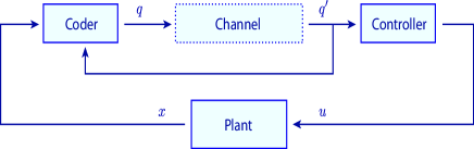
Figure 1: Control of a system over a noisy channel.

The source output is quantized as follows:

$$Q_{K}^{\Delta}(x)=\begin{cases}(k-{\mathchoice{\genfrac{}{}{}{1}{1}{2}}{\genfrac{}{}{}{1}{1}{2}}{\genfrac{}{}{}{3}{1}{2}}{\genfrac{}{}{}{3}{1}{2}}}(K+1))\Delta,\\ \quad\quad\quad\quad\quad\quad\mbox{if}x\in[(k-1-{\mathchoice{\genfrac{}{}{}{1}{1}{2}}{\genfrac{}{}{}{1}{1}{2}}{\genfrac{}{}{}{3}{1}{2}}{\genfrac{}{}{}{3}{1}{2}}}K)\Delta,(k-{\mathchoice{\genfrac{}{}{}{1}{1}{2}}{\genfrac{}{}{}{1}{1}{2}}{\genfrac{}{}{}{3}{1}{2}}{\genfrac{}{}{}{3}{1}{2}}}K)\Delta)\\ ({\mathchoice{\genfrac{}{}{}{1}{1}{2}}{\genfrac{}{}{}{1}{1}{2}}{\genfrac{}{}{}{3}{1}{2}}{\genfrac{}{}{}{3}{1}{2}}}(K-1))\Delta,\quad\quad\mbox{if}\ \ x={\mathchoice{\genfrac{}{}{}{1}{1}{2}}{\genfrac{}{}{}{1}{1}{2}}{\genfrac{}{}{}{3}{1}{2}}{\genfrac{}{}{}{3}{1}{2}}}K\Delta\\ 0,\quad\quad\mbox{if}\ \ x\not\in[-{\mathchoice{\genfrac{}{}{}{1}{1}{2}}{\genfrac{}{}{}{1}{1}{2}}{\genfrac{}{}{}{3}{1}{2}}{\genfrac{}{}{}{3}{1}{2}}}K\Delta,{\mathchoice{\genfrac{}{}{}{1}{1}{2}}{\genfrac{}{}{}{1}{1}{2}}{\genfrac{}{}{}{3}{1}{2}}{\genfrac{}{}{}{3}{1}{2}}}K\Delta]\end{cases}$$

where $K$ is a positive integer. The quantizer outputs are transmitted through a memoryless erasure channel, after being subjected to a bijective mapping, which is performed by the channel encoder. At time $t$, the channel encoder $\mathcal{E}_{t}$ maps the quantizer output symbols to corresponding channel inputs $q_{t}\in{\cal M}\mathbin{:=}\{1,2\dots,K+1\}$ so that ${\cal E}_{t}(Q_{t}(x_{t}))=q_{t}$. The controller/decoder has access to noisy versions of the encoder outputs $q^{\prime}_{t}\in\mathcal{M}^{\prime}\coloneqq{\cal M}\cup\{e\}$, with $e$ denoting the erasure symbol, generated according to a probability distribution for every fixed $q\in{\cal M}$. The channel transition probabilities are given by

$$P(q^{\prime}=i|q=i)=p,\quad\quad P(q^{\prime}=e|q=i)=1-p,\quad\quad i\in{\cal M}.$$

At each time $t$, the controller/decoder applies a mapping ${\cal D}_{t}:{\cal M}\cup\{e\}\to\mathbb{R}$, given by

$${\cal D}_{t}(q^{\prime}_{t})={\cal E}_{t}^{-1}(q^{\prime}_{t})\times 1_{\{q^{\prime}_{t}\neq e\}}+0\times 1_{\{q^{\prime}_{t}=e\}}.$$

Let $\{\Upsilon_{t}\}$ denote the sequence of i.i.d. binary random variables, representing the erasure process in the channel, where the event $\Upsilon_{t}=1$ indicates that the signal is transmitted with no error through the channel at time $t$. Let $p=E[\Upsilon_{t}]$ denote the probability of success in transmission. The following key assumptions are imposed: Given $K\geq 2$ introduced in the definition of the quantizer, define the rate variables

$$R=\log_{2}(K+1)\quad\quad R^{\prime}=\log_{2}(K)$$ (26)

We fix positive scalars $\delta$ and $\alpha$ satisfying $|a|2^{-R^{\prime}}<\alpha<1$ and $\alpha(|a|+\delta)^{p^{-1}-1}<1.$ With $L>0$ a constant, let $\bar{Q}:\mathbb{R}\times\mathbb{R}\times\{0,1\}\to\mathbb{R}$ be defined as

$$\bar{Q}(\Delta,h,p)=\begin{cases}|a|+\delta,&\text{ if }\quad|h|>1,\mbox{ or }p=0\\ \alpha,&\text{ if }0\leq|h|\leq 1,\;p=1,\;\Delta>L\\ 1,&\text{ if }0\leq|h|\leq 1,\;p=1,\;\Delta\leq L.\end{cases}$$

For each $t\geq 0$ and with $\Delta_{0}\in\mathbb{R}$ selected arbitrarily, let

$$u_{t} = -{a\over b}\hat{x}_{t},$$

$$\hat{x}_{t} = {\cal D}_{t}(q^{\prime}_{t})=\Upsilon_{t}Q_{K}^{\Delta_{t}}(x_{t}),$$

$$\Delta_{t+1} = \Delta_{t}\bar{Q}(\Delta_{t},|{x_{t}\over\Delta_{t}2^{R^{\prime}-1}}|,\Upsilon_{t}).$$ (27)

Given the channel output $q^{\prime}_{t}\neq e$, the controller can simultaneously deduce the realization of $\Upsilon_{t}$ and the event $\{|h_{t}|>1\}$, where $h_{t}=\frac{x_{t}}{\Delta_{t}2^{R^{\prime}-1}}$. This is due to the fact that if the channel output is not the erasure symbol, the controller knows that the signal is received with no error. If $q^{\prime}_{t}=e$, however, then the controller applies $0$ as its control input and enlarges the bin size of the quantizer.

By Lemma 3.1 of [11], $(x_{t},\Delta_{t})$ is a Markov chain.

Consider now a sequence of stopping times which denote the times when there is a successful transmission of a source symbol in the granular region of the quantizer:

$${\cal T}_{0}=0,\quad{\cal T}_{z+1} = \inf\{k>{\cal T}_{z}:|h_{k}|\leq 1,p_{k}=1\},\quad z\in\mathbb{Z}_{+}$$

By Proposition 3.1 of [11], the stopping time distribution is bounded uniformly by a geometric measure:

Lemma IV.1 ([11, Proposition 3.1]).

The discrete probability measure $P({\cal T}_{i+1}-{\cal T}_{i}=k\mid x_{{\cal T}_{i}},\Delta_{{\cal T}_{i}})$ satisfies,

$$(1-p)^{k-1}\leq P({\cal T}_{i+1}-{\cal T}_{i}\geq k\mid x_{{\cal T}_{i}},\Delta_{{\cal T}_{i}})\leq(1-p)^{k-1}+o(1),$$

where $o(1)\to 0$ as $\Delta_{{\cal T}_{i}}\to\infty$ uniformly in $x_{{\cal T}_{i}}$.

As a consequence, the probability $P({\cal T}_{i+1}-{\cal T}_{i}\geq k\mid x_{{\cal T}_{i}},\Delta_{{\cal T}_{i}})$ tends to $(1-p)^{k-1}p$ as $\Delta_{{\cal T}_{i}}\to\infty$.

Theorem IV.2.

Suppose that

$$a^{2}\Bigl{(}1-p+{p\over(2^{R}-1)^{2}}\Bigr{)}<1.$$ (28)

Then, under the coding and control policy considered, the chain $(x_{t},\Delta_{t})$ is geometrically ergodic.

Proof.

By the proof of Theorem 3.2 of [11], with $V(x,\Delta)=\Delta^{2}$, and with

$$0<\epsilon<1-{p\alpha^{2}\over 1-(1-p)(|a|+\delta)^{2}},$$

$b<\infty$ and $C$ a small set, it follows that

$$E[V(x_{{\cal T}_{z+1}},\Delta_{{\cal T}_{z+1}})\mid x_{{\cal T}_{z}}]$$

$$\leq(1-\epsilon)V(x_{{\cal T}_{z}},\Delta_{{\cal T}_{z}})+b1_{\{(x_{{\cal T}_{z}},\Delta_{{\cal T}_{z}})\in C\}}.$$ (29)

Together with Lemma IV.1, and (34) in [11] leading to (22), these imply that for some $\lambda=1-\epsilon\in(0,1)$, $B\in(p,{p\over\lambda})$ for some sufficiently large $C$, and $\beta=1-p$, Theorem III.7 holds.     $\sqcap$$\sqcup$

Remark IV.1.

We recall from [11] that under (28), the system is quadratically stable in the sense that for each initial condition $(x_{0},\Delta_{0})$, $\lim_{t\to\infty}E[x_{t}^{2}]=E_{\pi}[x_{0}^{2}]<\infty$. We also note that by [11] if the goal is to only have the existence of an invariant probability measure, the requirements on the channel reduce to the conditions that $|a|2^{-R^{\prime}}<\alpha<1$ and $\alpha(|a|+\delta)^{p^{-1}-1}<1.$

V Conclusion

In this paper, we established random-time state-dependent drift criteria for Markov chains using Lyapunov-theoretic methods. We established drift criteria both for sub-geometric and geometric rates of convergence, where the conditions revealed the relationship between the distributions of the stopping times, the drift of the Lyapunov functions at random times, and the ergodicity rates. Future work includes the application of these results in event triggered control systems, as well as information theory problems for variable-length decoding.

References

- [1] V. S. Borkar, “Convex analytic methods in Markov decision processes,” in Handbook of Markov Decision Processes, E. A. Feinberg, A. Shwartz (Eds.), pp. 347–375, Kluwer, Boston, MA, 2001.
- [2] S. P. Meyn, Control Techniques for Complex Networks. Cambridge University Press, 2007.
- [3] S. P. Meyn and R. Tweedie, Markov Chains and Stochastic Stability. London: Springer Verlag, 1993.
- [4] S. P. Meyn and R. Tweedie, “State-dependent criteria for convergence of Markov chains,” Ann. Appl. Prob, vol. 4, pp. 149–168, 1994.
- [5] V. A. Malyshev and M. V. Menshikov, “Ergodicity, continuity and analyticity of countable Markov chains,” Transactions Moscow Math. Soc, vol. 39, pp. 1–48, 1981.
- [6] S. B. Connor and G. Fort, “State-dependent Foster-Lyapunov criteria for subgeometric convergence of Markov chains,” Stoch. Process Appl., vol. 119, pp. 176–4193, 2009.
- [7] V. S. Borkar and S. P. Meyn, “The ODE method for convergence of stochastic approximation and reinforcement learning,” SIAM J. Control and Optimization, pp. 447–469, December 2000.
- [8] G. Fort, S. P. Meyn, E. Moulines, and P. Priouret, “ODE methods for skip-free Markov chain stability with applications to MCMC,” Annals of Applied Probability, pp. 664–707, 2008.
- [9] J. G. Dai, “On positive harris recurrence of multiclass queueing networks: a unified approach via fluid limit models,” Annals of Applied Probability, vol. 5, pp. 49–77, 1995.
- [10] J. G. Dai and S. P. Meyn, “Stability and convergence of moments for multiclass queueing networks via fluid limit models,” IEEE Transactions on Automatic Control, vol. 40, pp. 1889–1904, November 1995.
- [11] S. Yüksel and S. P. Meyn, “Random-time, state-dependent stochastic drift for Markov chains and application to stochastic stabilization over erasure channels,” IEEE Transactions on Automatic Control, vol. 58, pp. 47 – 59, January 2013.
- [12] B. H. Fralix, “Foster-type criteria for Markov chains on general spaces,” J. of Applied Probability, vol. 43, pp. 1194–1200, December 2006.
- [13] J. C. Kieffer, “Stochastic stability for feedback quantization schemes,” IEEE Transactions on Information Theory, vol. 28, pp. 248–254, March 1982.
- [14] J. C. Kieffer and J. G. Dunham, “On a type of stochastic stability for a class of encoding schemes,” IEEE Transactions on Information Theory, vol. 29, pp. 793–797, November 1983.
- [15] D. Liberzon and D. Nešić, “Input-to-state stabilization of linear systems with quantized state measurements,” IEEE Transactions on Automatic Control, vol. 52, pp. 767–781, May 2007.
- [16] R. Brockett and D. Liberzon, “Quantized feedback stabilization of linear systems,” IEEE Transactions on Automatic Control, vol. 45, pp. 1279–1289, July 2000.
- [17] G. N. Nair and R. J. Evans, “Stabilizability of stochastic linear systems with finite feedback data rates,” SIAM J. Control and Optimization, vol. 43, pp. 413–436, July 2004.
- [18] S. Yüksel, “Stochastic stabilization of noisy linear systems with fixed-rate limited feedback,” IEEE Transactions on Automatic Control, vol. 55, pp. 1014–1029, December 2010.
- [19] S. Yüksel and T. Başar, Stochastic Networked Control Systems: Stabilization and Optimization under Information Constraints. New York, NY: Springer-Birkhäuser, 2013.
- [20] M. Cloosterman, N. van de Wouw, W. Heemels, and H. Nijmeijer, “Stability of networked control systems with uncertain time-varying delays,” IEEE Transactions on Automatic Control, pp. 1575–1580, July 2009.
- [21] D. Quevedo, E. I. Silva, and G. C. Goodwin, “Control over unreliable networks affected by packet erasures and variable transmission delays,” IEEE J. on Selected Areas in Communications, vol. 26, pp. 672–685, 2008.
- [22] G. M. Lipsa and N. C. Martins, “Remote state estimation with communication costs for first-order LTI systems,” IEEE Transactions on Automatic Control, vol. 56, p. 2013 2025, September 2011.
- [23] W. Wu and A. Arapostathis, “Optimal sensor querying: General Markovian and LQG models with controlled observationss,” IEEE Transactions on Automatic Control, vol. 53, p. 1392 1405, July 2008.
- [24] K. J. Aström and B. Bernhardsson, “Comparison of Riemann and Lebesgue sampling for first order stochastic systems,” in Proceedings of the IEEE Conference on Decision and Control, pp. 2011–2016, December 2002.
- [25] D. Quevedo, V. Gupta, J. Ma, and S. Yüksel, “Stochastic stability of event-triggered anytime control,” IEEE Transactions on Automatic Control, vol. to appear.
- [26] K. J. M. Rabi and M. Johansson, “Optimal stopping for event-triggered sensing and actuation,” in Proceedings of the IEEE Conference on Decision and Control, pp. 3607–3612, December 2008.
- [27] M. Lemmon, “Event-triggered feedback in control, estimation, and optimization,” in Networked Control Systems, ser. Lecture Notes in Control and Information Sciences, A. Bemporad, M. Heemels, and M. Johansson, Eds., pp. 293–358, Springer Verlag, 2010.
- [28] P. Tabuada, “Event-triggered real-time scheduling of stabilizing control tasks,” IEEE Transactions on Automatic Control, vol. 52, pp. 1680–1685, September 2007.
- [29] O. Hernandez-Lerma and J. Lasserre, Discrete-time Markov control processes. Springer, 1996.
- [30] A. Arapostathis, V. S. Borkar, E. Fernandez-Gaucherand, M. K. Ghosh, and S. I. Marcus, “Discrete-time controlled Markov processes with average cost criterion: A survey,” SIAM J. Control and Optimization, vol. 31, pp. 282–344, 1993.
- [31] G. Roberts and J. Rosenthal, “General state space Markov chains and MCMC algorithms,” Probability Survery, vol. 1, pp. 20–71, 2004.
- [32] C. S. A. Antos and R. Munos, “Learning near-optimal policies with Bellman-residual minimization based fitted policy iteration and a single sample path,” Machine Learning, vol. 71, no. 1, pp. 89–129, 2008.
- [33] N. Saldi, T. Linder, and S. Yüksel, “Asymptotic optimality and rates of convergence of quantized stationary policies in stochastic control,” IEEE Trans. Automatic Control, vol. 60, pp. 553 –558, 2015.
- [34] R. A. Zurkowski, Lyapunov Analysis for Rates of Convergence in Markov Chains and Random-Time State-Dependent Drift. Queen’s University: MSc Thesis, 2013.
- [35] P. Tuominen and R. Tweedie, “Subgeometric rates of convergence of f-ergodic Markov chains,” Adv. Annals Appl. Prob., vol. 26, pp. 775–798, September 1994.
- [36] E. Nummelin, “A splitting technique for Harris recurrent Markov chains,” Z. Wahrscheinlichkeitstheoric verw. Gebiete, vol. 43, pp. 309–318, 1978.
- [37] K. B. Athreya and P. Ney, “A new approach to the limit theory of recurrent Markov chains,” Transactions of the American Mathematical Society, vol. 245, pp. 493–501, 1978.
- [38] M. Hairer, “Convergence of Markov processes.” lecture notes, University of Warwick, August, 2010, http://www.hairer.org/notes/Convergence.pdf.
- [39] R. Douc, G. Fort, E. Moulines, and P. Soulier, “Practical drift conditions for subgeometric rates of convergence,” Ann. Appl. Probab, vol. 14, pp. 1353–1377, 2004.