Direct observation of any two-point quantum correlation function

Abstract

The existence of noncompatible observables in quantum theory makes a direct operational interpretation of two-point correlation functions problematic. Here we challenge such a view by explicitly constructing a measuring scheme that, independently of the input state $\rho$ and observables $A$ and $B$, performs an unbiased optimal estimation of the two-point correlation function $\operatorname{Tr}[A\ \rho\ B]$. This shows that, also in quantum theory, two-point correlation functions are as operational as any other expectation value. A very simple probabilistic implementation of our proposal is presented.

In the description of stochastic physical processes, it is important to determine how dynamical variables are correlated with each other. Correlation functions are computed as products of two (or more) dynamical variables (or their powers), averaged over time, or over many sites, or in both ways. In the simplest case of the average of the product of two dynamical variables, one usually speaks of two-point correlation functions.

In classical physics, dynamical variables are real-valued functions of the state of the system. In fact, the state of the system can be fully specified, in principle, by giving the values of all its dynamical variables (or its generating set of variables), at any instant in time. In classical statistical mechanics, therefore, there is no difficulty in defining and computing correlation functions, however complicated, between dynamical variables; as dynamical variables are all experimentally accessible, so are all correlation functions.

In quantum mechanics, on the contrary, the relation between states and dynamical variables is much more subtle. In particular, the notion of dynamical variables is replaced by that of observables, namely, self-adjoint operators that can or cannot commute; this is the formal reason for the existence of “incompatible” variables that cannot simultaneously assume definite values in any state uncertanty . This feature arguably lies at the origin of all “quantum spooks,” including a prevailing view that correlation functions are typically ill-defined for a quantum mechanical system — if two observables do not both have a definite value simultaneously, how could one compute the average of their product then?

Interpretational problems notwithstanding, one still can formally define two-point quantum correlation functions as $\operatorname{Tr}[A\ \rho\ B]$, where $\rho$ describes the state of the system and $A$, $B$ are any two observables (or, possibly, the same observable at different times, in which case we more precisely speak of auto-correlation functions). In fact, such functions are extensively used in a wide variety of fields, such as quantum statistical mechanics quant-stat , quantum thermodynamics quant-term , and quantum field theory quant-field . The question then naturally arises, whether quantum correlation functions can be given a clear operational interpretation.

For the sake of concreteness, suppose we are given a source, in control, emitting independent systems, all of them in the same (though unknown) state. We are also given two measuring apparatuses, as accurate as the theory (classical or quantum) allows, one to measure observable $A$, the other for observable $B$. We assume that both apparatuses can be initialized and re-used an arbitrary number of times. In classical physics, these assumptions are enough to allow us to measure, in principle, not only the expected values of $A$ and $B$, but also any moment of these, i.e. any two-point correlation function. This is possible because, classically, measurement does not imply disturbance. Therefore, one can perform successive measurements of $A$ and $B$ on the same system, collect the results, and post-process them at will. For example, auto-correlation functions in classical physics are computed by measuring a certain observable twice on the same system, at different times. On the other hand, in quantum theory, such a simple approach is often impossible due to the existence of incompatible observables, as a measurement done now unavoidably disturbs the evolution of the system and, therefore, the result of a measurement performed on the system at later times, unless the measurement satisfies quantum non-demolition conditions; see for instance Ref. CTDSZ80 .

For this reason it seems that two-point correlation functions (and auto-correlation functions, in particular) cannot be interpreted operationally in quantum theory, in the sense that they cannot be directly measured experimentally. In this paper we argue that this would be too hurried a conclusion. Our contribution is to construct a “black-box”–like approach to quantum correlation functions, working for (but being independent of) any state $\rho$ and any pair of observables $A$ and $B$ (see Fig. 1 below).

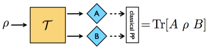
Figure 1: The ideal two-point correlator described as a black-box, labeled by $\mathcal{T}$. The quantum system, in state $\rho$, is fed into the black-box. The output consists of two quantum systems, on which independent measurements of observables $A$ and $B$ are performed. The data collected are then recombined by a purely classical post-processing, resulting in the value $\operatorname{Tr}[A\ \rho\ B]$. Notice that both the black-box $\mathcal{T}$ and the final classical post-processing are independent of $\rho$, $A$ and $B$. In this sense, the black-box $\mathcal{T}$ and the post-processing are universal.

First, the quantum system of interest is fed through a black-box $\mathcal{T}$, what we call the “ideal two-point correlator.” The black-box in turns produces two output systems, on which the two observables $A$ and $B$ can be independently measured, even if they were incompatible. The recorded values are finally post-processed according to a fixed post-processing function such that, if the system was initially prepared in state $\rho$, the average result equals $\operatorname{Tr}[A\ \rho\ B]$. Since both the quantum black-box and the classical post-processing are independent of $\rho$, $A$, and $B$, our scheme shows that quantum two-point correlation functions are no less operational than any other expectation value, challenging the common understanding explained above and suggesting, at the same time, new experimental procedures to directly measure them.

In the rest of the paper, we will explicitly construct the black-box and the post-processing function allowing the experimental assessment of any two-point quantum correlation function of the form $\operatorname{Tr}[A\ \rho\ B]$, for any state $\rho$ and any pair of observables $A$ and $B$. Remarkably, both the quantum pre-processing and the classical post-processing will be independent of $\rho$, $A$ and $B$, thus providing a universal strategy. We will also prove that our strategy is optimal, for any state $\rho$ and any observables $A$ and $B$, in the sense that it always minimizes the error propagation due to the final post-processing of data. We will finally present a very simple probabilistic implementation of our proposal on qubits encoded in the polarization of photons.

Notation and basic concepts.—In what follows, we will only consider quantum systems defined on finite dimensional Hilbert spaces, denoted by ${\mathcal{H}}$ and ${\mathcal{K}}$, with dimensions $d_{\mathcal{H}}$ and $d_{\mathcal{K}}$, respectively. The set of all linear operators mapping elements in ${\mathcal{H}}$ to elements in ${\mathcal{K}}$ will be denoted by $\boldsymbol{\mathsf{L}}({\mathcal{H}},{\mathcal{K}})$, with the convention that $\boldsymbol{\mathsf{L}}({\mathcal{H}}):=\boldsymbol{\mathsf{L}}({\mathcal{H}},{\mathcal{H}})$. We will denote by $\boldsymbol{\mathsf{S}}({\mathcal{H}})$ the set of all density matrices (or states), namely all those operators $\rho\in\boldsymbol{\mathsf{L}}({\mathcal{H}})$ such that $\rho\geqslant 0$ and $\operatorname{Tr}[\rho]=1$. The identity matrix in $\boldsymbol{\mathsf{L}}({\mathcal{H}})$ will be denoted by the symbol $\mathds{1}$. In the proofs of our statements, which are collected in the Supplemental material, we will make use of well established mathematical results introduced in choi ; stine .

Formalization.—We define the ideal two-point quantum correlator as the linear transformation ${\mathcal{T}}:\boldsymbol{\mathsf{L}}({\mathcal{H}})\to\boldsymbol{\mathsf{L}}({\mathcal{H}}\otimes{\mathcal{H}})$, which acts in such a way that the following equation,

$$\operatorname{Tr}[\mathcal{T}(\rho)\ (A\otimes B)]:=\operatorname{Tr}[A\ \rho\ B],$$ (1)

is satisfied for all input states $\rho\in\boldsymbol{\mathsf{S}}({\mathcal{H}})$ and all observables $A,B\in\boldsymbol{\mathsf{L}}({\mathcal{H}})$. Defining the swap operator $S\in\boldsymbol{\mathsf{L}}({\mathcal{H}}\otimes{\mathcal{H}})$ by $S|\phi,\chi\rangle=|\chi,\phi\rangle$ for all $\phi,\chi\in{\mathcal{H}}$, the above equation is equivalent to the following:

$$\mathcal{T}(\rho)=S(\mathds{1}_{\mathcal{H}}\otimes\rho),$$ (2)

for all $\rho\in\boldsymbol{\mathsf{S}}({\mathcal{H}})$. Relation (2) above makes apparent that, on one hand, the map ${\mathcal{T}}$ is linear, but also, on the other, that ${\mathcal{T}}$ is not a physical evolution. Such a conclusion is a direct consequence of the fact that ${\mathcal{T}}$ does not preserves hermiticity, which is a necessary condition for complete positivity.

However, as we will show in the rest of the paper, even if the map ${\mathcal{T}}$ cannot be realized as a physical evolution, it can, nonetheless, be given a well motivated operational interpretation and an experimentally feasible realization scheme, in terms of partial expectation values, a concept that we will introduce in Proposition 2.

Before proceeding, we make the following simple observation. The product of two observables can always be decomposed as the linear combination of two self-adjoint operators, namely:

$$BA=\frac{\{A,B\}}{2}-\operatorname{\imath}\frac{[A,B]}{2\operatorname{\imath}},$$

where $\{A,B\}:=AB+BA$ and $[A,B]:=AB-BA$ are the anti-commutator and commutator, respectively, and $\operatorname{\imath}$ denotes the imaginary unit. By linearity then, any two-point correlation function can be rewritten as

$$\operatorname{Tr}[A\ \rho\ B]=\operatorname{Tr}\left[\rho\ \frac{\{A,B\}}{2}\right]-\operatorname{\imath}\operatorname{Tr}\left[\rho\ \frac{[A,B]}{2\operatorname{\imath}}\right].$$

The above decomposition directly induces an analogous decomposition of the map $\mathcal{T}$ into its real and imaginary parts:

$$\mathcal{T}=\mathcal{R}-\operatorname{\imath}\mathcal{I},$$ (3)

where $\mathcal{R}:\boldsymbol{\mathsf{L}}({\mathcal{H}})\to\boldsymbol{\mathsf{L}}({\mathcal{H}}\otimes{\mathcal{H}})$ and $\mathcal{I}:\boldsymbol{\mathsf{L}}({\mathcal{H}})\to\boldsymbol{\mathsf{L}}({\mathcal{H}}\otimes{\mathcal{H}})$ are defined by

$$\operatorname{Tr}[\mathcal{R}(\rho)\ (A\otimes B)]:=\operatorname{Tr}\left[\rho\ \frac{\{A,B\}}{2}\right],$$ (4)

and

$$\operatorname{Tr}[\mathcal{I}(\rho)\ (A\otimes B)]:=\operatorname{Tr}\left[\rho\ \frac{[A,B]}{2\operatorname{\imath}}\right],$$ (5)

for all $\rho,A,B$. We notice that, as it was the case for ${\mathcal{T}}$, both $\mathcal{R}$ and $\mathcal{I}$ are linear transformations. Contrarily to ${\mathcal{T}}$, however, they are now both hermiticity-preserving (HP). Finally, the map $\mathcal{R}$ is easily seen to be also trace-preserving (TP), while $\operatorname{Tr}[\mathcal{I}(\rho)]=0$, for all $\rho\in\boldsymbol{\mathsf{S}}({\mathcal{H}})$.

Statistical decompositions and partial expectation values.—Suppose that, given a linear HP map $\mathcal{L}:\boldsymbol{\mathsf{L}}(\mathcal{H})\to\boldsymbol{\mathsf{L}}(\mathcal{K})$, one wants to find a way to experimentally measure the expectation value $\operatorname{Tr}[\mathcal{L}(\rho)\ A]$, for any input state $\rho\in\boldsymbol{\mathsf{S}}(\mathcal{H})$ and any observable $A\in\boldsymbol{\mathsf{L}}(\mathcal{K})$. The following proposition, proved in the Supplemental material, provides a way to do so.

Proposition 1 (Statistical Decompositions).

Any hermiticity-preserving linear map ${\mathcal{L}}:\boldsymbol{\mathsf{L}}({\mathcal{H}})\to\boldsymbol{\mathsf{L}}({\mathcal{K}})$ can be decomposed as ${\mathcal{L}}=\sum_{i}\lambda_{i}{\mathcal{E}}_{i}$ for suitable real coefficients $\lambda_{i}$, where ${\mathcal{E}}_{i}:\boldsymbol{\mathsf{L}}({\mathcal{H}})\to\boldsymbol{\mathsf{L}}({\mathcal{K}})$ are completely positive for all $i$, and ${\mathcal{E}}:=\sum_{i}{\mathcal{E}}_{i}$ is trace-preserving. [Namely, the collection $\{{\mathcal{E}}_{i}\}_{i}$ constitutes a quantum instrument instrument .]

The content of Proposition 1 is summarized in Fig. 2 below: for any linear HP map $\mathcal{L}:\boldsymbol{\mathsf{L}}(\mathcal{H})\to\boldsymbol{\mathsf{L}}(\mathcal{K})$, there exist a quantum instrument $\{\mathcal{E}_{i}\}_{i}$, with $\mathcal{E}_{i}:\boldsymbol{\mathsf{L}}(\mathcal{H})\to\boldsymbol{\mathsf{L}}(\mathcal{K})$ CP for all $i$, and real coefficients $\lambda_{i}$, such that

$$\operatorname{Tr}[\mathcal{L}(\rho)\ A]=\sum_{i}\lambda_{i}\operatorname{Tr}[\mathcal{E}_{i}(\rho)\ A],$$ (6)

for any input state $\rho$ and any observable $A$. Such a decomposition will be referred to as a statistical decomposition of the map ${\mathcal{L}}$.

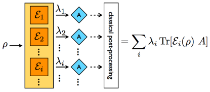
Figure 2: Statistical decomposition of a non-physical transformation: (1) the initial state $\rho$ goes through a quantum instrument, described by a collection of CP maps ${\mathcal{E}}_{i}$; (2) the outcome $i$, occurring with probability $p(i)=\operatorname{Tr}[{\mathcal{E}}_{i}(\rho)]$, is recorded; (3) the corresponding output state $\rho_{i}={\mathcal{E}}_{i}(\rho)/p(i)$ is used to evaluate the expectation value $\langle A\rangle_{i}=\operatorname{Tr}[\rho_{i}\ A]$; (4) all data are finally recombined as $\sum_{i}\lambda_{i}p(i)\langle A\rangle_{i}$, for suitable real coefficients $\lambda_{i}$.

It is important now to notice that, while Proposition 1 above shows that there always exists at least one statistical decomposition for every linear HP map, statistical decompositions, as in (6), are in general highly non-unique. In order to single out an optimal decomposition, an optimality criterion must be introduced. A natural choice for the optimality criterion is the statistical error statistics on the expectation value $\operatorname{Tr}[\mathcal{L}(\rho)A]$. To define it formally let us rewrite Eq. (6) as follows

$$\operatorname{Tr}[\mathcal{L}(\rho)\ A] =\sum_{i}\lambda_{i}p(i)\operatorname{Tr}[\rho_{i}\ A]$$

$$=\sum_{i}\lambda_{i}p(i)\langle A\rangle_{i},$$ (7)

where $p(i):=\operatorname{Tr}[{\mathcal{E}}_{i}(\rho)]$, $\rho_{i}:=p(i)^{-1}{\mathcal{E}}_{i}(\rho)$, and $\langle A\rangle_{i}:=\operatorname{Tr}[\rho_{i}\ A]$. Since the expectation values $\langle A\rangle_{i}$ all come with their own statistical error, say $\varepsilon_{i}$, one has that the error associated with the linear combination (Direct observation of any two-point quantum correlation function) is conservatively evaluated as $\sum_{i}|\lambda_{i}|p(i)\varepsilon_{i}$. For this reason, we choose to adopt here the rather conservative criterion of minimizing $\sum_{i}|\lambda_{i}|p(i)$, for all input states $\rho$.

The following representation theorem (proved in the Supplemental material) provides an alternative way to interpret statistical decompositions as partial expectation values (not to be confused with the well-established notion of conditional expectation values):

Proposition 2 (Partial Expectation Values).

For any linear HP map ${\mathcal{L}}:\boldsymbol{\mathsf{L}}({\mathcal{H}})\to\boldsymbol{\mathsf{L}}({\mathcal{K}})$, there exists a finite dimensional ancillary quantum system ${\mathcal{K}}^{\prime}$, an isometry $V:{\mathcal{H}}\to{\mathcal{K}}\otimes{\mathcal{K}}^{\prime}$ and an observable $Z\in\boldsymbol{\mathsf{L}}({\mathcal{K}}^{\prime})$, such that

$$\operatorname{Tr}[V\rho V^{\dagger}\ (A\otimes Z)]=\operatorname{Tr}[{\mathcal{L}}(\rho)\ A],$$ (8)

for all states $\rho\in\boldsymbol{\mathsf{S}}({\mathcal{H}})$ and all observables $A\in\boldsymbol{\mathsf{L}}({\mathcal{K}})$. Equivalently,

$${\mathcal{L}}(\rho)=\operatorname{Tr}_{{\mathcal{K}}^{\prime}}[V\rho V^{\dagger}\ (\mathds{1}\otimes Z)],$$ (9)

namely, the action of ${\mathcal{L}}$ can be written as a “partial expectation value.”

The idea of partial expectation values is depicted in Fig. 3 below.

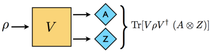
Figure 3: Statistical decompositions as partial expectation values: according to Proposition 2, $\operatorname{Tr}[V\rho V^{\dagger}\ (A\otimes Z)]=\operatorname{Tr}[{\mathcal{L}}(\rho)\ A]$, for all input states $\rho$ and all final observables $A$. Notice that the isometry $V$ and the ancillary observable $Z$ do not depend neither on the input state $\rho$ nor on the final observable $A$, but only on the linear HP map ${\mathcal{L}}$.

Universal optimal two-point quantum correlator.—The proofs of the following Propositions can be found in the Supplemental material.

Proposition 3 (Universal Optimal Statistical Decomposition of $\mathcal{R}$).

The map $\mathcal{R}:\boldsymbol{\mathsf{L}}({\mathcal{H}})\to\boldsymbol{\mathsf{L}}({\mathcal{H}}\otimes{\mathcal{H}})$ representing the real part of the ideal two-point correlator $\mathcal{T}$, as in Eqs. (3) and (4), admits a statistical decomposition, which is universally optimal, i.e. optimal at once for any input state $\rho\in\boldsymbol{\mathsf{S}}({\mathcal{H}})$, namely

$$\mathcal{R}=\frac{d_{\mathcal{H}}+1}{2}\mathcal{R}_{+}-\frac{d_{\mathcal{H}}-1}{2}\mathcal{R}_{-}.$$ (10)

In the above equation, $\mathcal{R}_{+}$ and $\mathcal{R}_{-}$ are, respectively, the symmetric and anti-symmetric $1\to 2$ optimal cloners defined, for any $\rho\in\boldsymbol{\mathsf{L}}({\mathcal{H}})$, as follows werner :

$$\mathcal{R}_{\pm}(\rho):=\frac{2}{d_{\mathcal{H}}\pm 1}P^{\pm}\left(\mathds{1}_{\mathcal{H}}\otimes\rho\right)P^{\pm},$$

where $P^{+}$ and $P^{-}$ are the projectors on, respectively, the symmetric and antisymmetric subspaces of ${\mathcal{H}}\otimes{\mathcal{H}}$, namely, $P^{\pm}=\frac{1}{2}(\mathds{1}\pm S)$ being $S\in\boldsymbol{\mathsf{L}}({\mathcal{H}}\otimes{\mathcal{H}})$ the swap operator.

Proposition 4 (Universal Optimal Statistical Decomposition of $\mathcal{I}$).

The map $\mathcal{I}:\boldsymbol{\mathsf{L}}({\mathcal{H}})\to\boldsymbol{\mathsf{L}}({\mathcal{H}}\otimes{\mathcal{H}})$ representing the imaginary part of the ideal two-point correlator $\mathcal{T}$, as in Eqs. (3) and (5), admits a statistical decomposition, which is universally optimal, i.e. optimal at once for any input state $\rho\in\boldsymbol{\mathsf{S}}({\mathcal{H}})$, namely

$$\mathcal{I}=\frac{\sqrt{d_{\mathcal{H}}^{2}-1}}{2}\mathcal{I}_{+}-\frac{\sqrt{d_{\mathcal{H}}^{2}-1}}{2}\mathcal{I}_{-}.$$ (11)

In the above equation, $\mathcal{I}_{+}$ and $\mathcal{I}_{-}$ are defined, for any $\rho\in\boldsymbol{\mathsf{L}}({\mathcal{H}})$, as follows:

$$\mathcal{I}_{\pm}(\rho):=\frac{2d_{\mathcal{H}}}{(d_{\mathcal{H}}^{2}-1)}Q^{\pm}\left(\mathds{1}_{\mathcal{H}}\otimes\rho\right)Q^{\mp},$$

where $Q^{+}=(Q^{-})^{\dagger}:=\frac{1}{2}(\mathds{1}+zS)$, being $S\in\boldsymbol{\mathsf{L}}({\mathcal{H}}\otimes{\mathcal{H}})$ the swap operator and $z=(-1+\operatorname{\imath}\sqrt{d_{\mathcal{H}}^{2}-1})/d_{\mathcal{H}}$ a complex phase.

Conclusions.—In this work we provided two point correlation functions with a new operational interpretation. We did this by explicitly constructing a “universal optimal two-point quantum correlator,” namely, a measuring apparatus which, independently of $\rho$, $A$, and $B$, performs an unbiased optimal (in a statistical sense) estimation of the ideal two-point correlation function $\operatorname{Tr}[A\ \rho\ B]$. This proves that, despite the interpretational difficulties due to noncommutativity of $A$ and $B$, two-point correlation functions are as operational as any other expectation value.

We conclude with a proposal for an experiment probabilitistically implementing the real part $\mathcal{R}$ of the universal two-point correlator. Our proposal is depicted in Fig. 4 in the case of qubits encoded on photons polarization. (The case of the imaginary part $\mathcal{I}$ is more involved: an approximate experimental implementation, rigorous only in the limit $d\to\infty$, will be discussed elsewhere, based on results in Ref. CSBDF08 ).

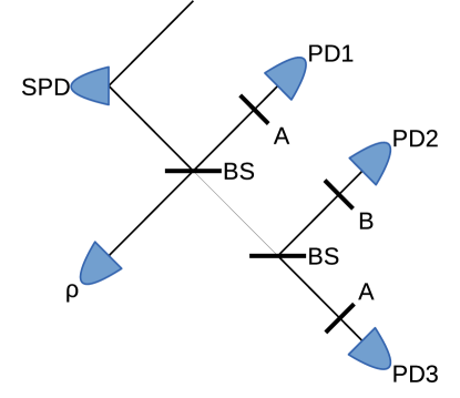
Figure 4: Experimental proposal for the probabilistic implementation of the real part of the universal optimal two-point correlator for qubits. Thin lines represent optical qubits encoded in the polarization of photons, BS is a $50/50$ beamsplitter, SPD is a source of maximally entangled photons through spontaneous parametric downconversion, $\rho$ is the input state fed into the universal optimal two-point correlator, $A$ and $B$ are the phase shifters implementing the corresponding observables, PD1, PD2, and PD3 are photodetectors. A coincidence occurs between PD2 and PD3 (resp., PD1 and PD2) with probability $3/16$ (resp., $1/16$), in this case optimal universal symmetric (resp., antisymmetric) cloning has been performed. Other cases are discarded. Averaging over the output statistics with the weights given by Eq. (10), one recovers the correlation function $\operatorname{Tr}[A\ \rho\ B]$.

The system first interacts with a maximally entangled photon generated by spontaneous parametric downconversion on a $50/50$ beamsplitter. One of the two output modes is further splitted by another $50/50$ beamsplitter. Finally, phase shifters, corresponding to operators $A$ and $B$, are applied on each output mode, and photodetection is performed (preceded by polarizing beamsplitters in order to spatially separate the two polarizations). Despite the present experimental proposal covers only the case of the real part (corresponding, as per Eq. (4), to the anti-commutator $\{A,B\}$), it is already enough to provide new experimental tests of noise-disturbance relations exper-noise-dist and quantumness witnesses quantumness .

F. B. was supported by the Program for Improvement of Research Environment for Young Researchers from Special Coordination Funds for Promoting Science and Technology (SCF) commissioned by the Ministry of Education, Culture, Sports, Science and Technology (MEXT) of Japan. M. D. was supported by JSPS (Japan Society for the Promotion of Science) Grant-in-Aid for JSPS Fellows No. 24-0219. M. O. is supported by the John Templeton Foundations, ID #35771, and MIC SCOPE, No. 121806010. This work is supported by JSPS KAKENHI, No. 21244007.

Supplemental material

In what follows, we will only consider quantum systems defined on finite dimensional Hilbert spaces, denoted by ${\mathcal{H}}$ and ${\mathcal{K}}$, with dimensions $d_{\mathcal{H}}$ and $d_{\mathcal{K}}$, respectively. The set of all linear operators mapping elements in ${\mathcal{H}}$ to elements in ${\mathcal{K}}$ will be denoted by $\boldsymbol{\mathsf{L}}({\mathcal{H}},{\mathcal{K}})$, with the convention that $\boldsymbol{\mathsf{L}}({\mathcal{H}}):=\boldsymbol{\mathsf{L}}({\mathcal{H}},{\mathcal{H}})$. We will denote by $\boldsymbol{\mathsf{S}}({\mathcal{H}})$ the set of all density matrices (or states), namely all those operators $\rho\in\boldsymbol{\mathsf{L}}({\mathcal{H}})$ such that $\rho\geqslant 0$ and $\operatorname{Tr}[\rho]=1$. The identity matrix in $\boldsymbol{\mathsf{L}}({\mathcal{H}})$ will be denoted by the symbol $\mathds{1}$. The term observable will be used as a synonim of self-adjoint operator. The identity map on $\boldsymbol{\mathsf{L}}(\mathcal{H})$ will be denoted by $\mathsf{id}$. The maximally entangled state $d^{-1}\sum_{i,j}|i,i\rangle\langle j,j|$ will be denoted by $\Phi^{+}$. The swap operator will be denoted by $S$, namely $S\in\boldsymbol{\mathsf{L}}(\mathcal{H}\otimes\mathcal{H})$ is the unitary self-adjoint operator acting as $S|\psi,\phi\rangle=|\phi,\psi\rangle$, for all $|\psi\rangle,|\phi\rangle\in\mathcal{H}$. The projectors on the symmetric and antisymmetric subspaces will be denoted by $P_{\pm}=\frac{1}{2}(\mathds{1}\pm S)$, respectively.

Given a linear map ${\mathcal{L}}:\boldsymbol{\mathsf{L}}({\mathcal{H}})\to\boldsymbol{\mathsf{L}}({\mathcal{K}})$, the so-called Choi isomorphism choi provides a way to associate ${\mathcal{L}}$ with an operator $\boldsymbol{\mathsf{C}}\!\left[{{\mathcal{L}}}\right]\in\boldsymbol{\mathsf{L}}({\mathcal{K}}\otimes{\mathcal{H}})$, whose matrix, in the standard representation given by the computational basis $\{|k\rangle\}$, is defined as

$$\boldsymbol{\mathsf{C}}\!\left[{{\mathcal{L}}}\right]:=d({\mathcal{L}}\otimes\mathsf{id})(|\Phi^{+}\rangle\langle\Phi^{+}|),$$ (12)

being $|\Phi^{+}\rangle$ the standard maximally entangled state introduced above. The inverse correspondence works as follows: given an operator $J\in\boldsymbol{\mathsf{L}}({\mathcal{K}}\otimes{\mathcal{H}})$, the Choi isomorphism constructs a linear map $\boldsymbol{\mathsf{C}}^{-1}\!\left[{J}\right]:\boldsymbol{\mathsf{L}}({\mathcal{H}})\to\boldsymbol{\mathsf{L}}({\mathcal{K}})$ defined, for all $M\in\boldsymbol{\mathsf{L}}({\mathcal{H}})$, by

$$\boldsymbol{\mathsf{C}}^{-1}\!\left[{J}\right](M):=\operatorname{Tr}_{\mathcal{H}}\left[J\ (\mathds{1}_{{\mathcal{K}}}\otimes M^{T})\right],$$ (13)

where the exponent $T$ denotes the transposition with respect to the computational basis $\{|k\rangle\}$. The importance of the Choi isomorphism lies in the following three properties:

1. linearity, i.e. $\boldsymbol{\mathsf{C}}\!\left[{a{\mathcal{L}}+b{\mathcal{L}}^{\prime}}\right]=a\boldsymbol{\mathsf{C}}\!\left[{{\mathcal{L}}}\right]+b\boldsymbol{\mathsf{C}}\!\left[{{\mathcal{L}}^{\prime}}\right]$ and $\boldsymbol{\mathsf{C}}^{-1}\!\left[{aJ+bJ^{\prime}}\right]=a\boldsymbol{\mathsf{C}}^{-1}\!\left[{J}\right]+b\boldsymbol{\mathsf{C}}^{-1}\!\left[{J^{\prime}}\right]$;

2. bijectivity, i.e. $\boldsymbol{\mathsf{C}}^{-1}\!\left[{\boldsymbol{\mathsf{C}}\!\left[{{\mathcal{L}}}\right]}\right]={\mathcal{L}}$ and $\boldsymbol{\mathsf{C}}\!\left[{\boldsymbol{\mathsf{C}}^{-1}\!\left[{J}\right]}\right]=J$;

3. finally, and more importantly, the map ${\mathcal{L}}$ is completely positive (CP) if and only if the corresponding operator $\boldsymbol{\mathsf{C}}\!\left[{{\mathcal{L}}}\right]$ is non-negative.

Other properties, which follow easily from the definition, are the following:

1. the map ${\mathcal{L}}$ is hermiticity-preserving (HP), if and only if the corresponding operator $\boldsymbol{\mathsf{C}}\!\left[{{\mathcal{L}}}\right]$ is hermitian;

2. the map ${\mathcal{L}}$ is trace-preserving (TP), if and only if the corresponding operator $\boldsymbol{\mathsf{C}}\!\left[{{\mathcal{L}}}\right]$ satisfies the normalization condition $\operatorname{Tr}_{{\mathcal{K}}}[\boldsymbol{\mathsf{C}}\!\left[{{\mathcal{L}}}\right]]=\mathds{1}_{\mathcal{H}}$.

We now prove Proposition 1, that we restate here for convenience.

Proposition 5 (Statistical Decompositions).

Any hermiticity-preserving linear map ${\mathcal{L}}:\boldsymbol{\mathsf{L}}({\mathcal{H}})\to\boldsymbol{\mathsf{L}}({\mathcal{K}})$ can be decomposed as ${\mathcal{L}}=\sum_{i}\lambda_{i}{\mathcal{E}}_{i}$ for suitable coefficients $\lambda_{i}\in\mathbb{R}$, where ${\mathcal{E}}_{i}:\boldsymbol{\mathsf{L}}({\mathcal{H}})\to\boldsymbol{\mathsf{L}}({\mathcal{K}})$ are completely positive for all $i$, and ${\mathcal{E}}:=\sum_{i}{\mathcal{E}}_{i}$ is trace-preserving.

Proof.

We already saw that the operator $\boldsymbol{\mathsf{C}}\!\left[{{\mathcal{L}}}\right]\in\boldsymbol{\mathsf{L}}({\mathcal{K}}\otimes{\mathcal{H}})$ is hermitian, whenever the map ${\mathcal{L}}$ is HP. We can therefore diagonalize $\boldsymbol{\mathsf{C}}\!\left[{{\mathcal{L}}}\right]$ as $\boldsymbol{\mathsf{C}}\!\left[{{\mathcal{L}}}\right]=\sum_{i}\mu_{i}\Pi_{i}$, with $\mu_{i}\in\mathbb{R}$ and $\Pi_{i}$ orthogonal projectors such that $\sum_{i}\Pi_{i}=\mathds{1}_{{\mathcal{K}}}\otimes\mathds{1}_{{\mathcal{H}}}$. The statement is recovered simply by normalizing by $d_{\mathcal{K}}$, namely, $\lambda_{i}:=d_{\mathcal{K}}\mu_{i}$, and ${\mathcal{E}}_{i}:=\boldsymbol{\mathsf{C}}^{-1}\!\left[{d_{\mathcal{K}}^{-1}\Pi_{i}}\right]$. ∎

The following Lemma provides a lower bound on the statistical error $\sum_{i}|\lambda_{i}|p(i)$, with $p(i):=\operatorname{Tr}[{\mathcal{E}}_{i}(\rho)]$, associated to statistical decomposition ${\mathcal{L}}=\sum_{i}\lambda_{i}{\mathcal{E}}_{i}$.

Lemma 1.

Given a HP linear map ${\mathcal{L}}:\boldsymbol{\mathsf{L}}({\mathcal{H}})\to\boldsymbol{\mathsf{L}}({\mathcal{K}})$, for any statistical decomposition ${\mathcal{L}}=\sum_{i}\lambda_{i}{\mathcal{E}}_{i}$ and any input state $\rho\in\boldsymbol{\mathsf{S}}({\mathcal{H}})$,

$$\sum_{i}|\lambda_{i}|p(i)\geqslant\min_{\sigma\in\boldsymbol{\mathsf{S}}({\mathcal{H}})}\operatorname{Tr}\left[|\boldsymbol{\mathsf{C}}\!\left[{{\mathcal{L}}}\right]|\ (\mathds{1}_{\mathcal{K}}\otimes\sigma)\right],$$ (14)

where $p(i):=\operatorname{Tr}[{\mathcal{E}}_{i}(\rho)]$.

Proof.

For any statistical decomposition ${\mathcal{L}}=\sum_{i}\lambda_{i}{\mathcal{E}}_{i}$, the linearity of the Choi isomorphism implies that $\boldsymbol{\mathsf{C}}\!\left[{{\mathcal{L}}}\right]=\sum_{i}\lambda_{i}\boldsymbol{\mathsf{C}}\!\left[{{\mathcal{E}}_{i}}\right]$. This implies that $|\boldsymbol{\mathsf{C}}\!\left[{{\mathcal{L}}}\right]|\leqslant\sum_{i}|\lambda_{i}|\boldsymbol{\mathsf{C}}\!\left[{{\mathcal{E}}_{i}}\right]$, which in turn implies $\operatorname{Tr}\left[|\boldsymbol{\mathsf{C}}\!\left[{{\mathcal{L}}}\right]|\ (\mathds{1}_{\mathcal{K}}\otimes\sigma)\right]\leqslant\sum_{i}|\lambda_{i}|\operatorname{Tr}\left[\boldsymbol{\mathsf{C}}\!\left[{{\mathcal{E}}_{i}}\right]\ (\mathds{1}_{\mathcal{K}}\otimes\sigma)\right]$ for all $\sigma\geqslant 0$. The statement is recovered by minimizing over $\sigma$ the left-hand side. ∎

We now prove Proposition 2, that we restate for convenience.

Proposition 6 (Partial Expectation Values).

For any linear HP map ${\mathcal{L}}:\boldsymbol{\mathsf{L}}({\mathcal{H}})\to\boldsymbol{\mathsf{L}}({\mathcal{K}})$, there exists a finite dimensional ancillary quantum system ${\mathcal{K}}^{\prime}$, an isometry $V:{\mathcal{H}}\to{\mathcal{K}}\otimes{\mathcal{K}}^{\prime}$ and an observable $Z\in\boldsymbol{\mathsf{L}}({\mathcal{K}}^{\prime})$, such that

$$\operatorname{Tr}[V\rho V^{\dagger}\ (A\otimes Z)]=\operatorname{Tr}[{\mathcal{L}}(\rho)\ A],$$ (15)

for all states $\rho\in\boldsymbol{\mathsf{S}}({\mathcal{H}})$ and all observables $A\in\boldsymbol{\mathsf{L}}({\mathcal{K}})$. Equivalently,

$${\mathcal{L}}(\rho)=\operatorname{Tr}_{{\mathcal{K}}^{\prime}}[V\rho V^{\dagger}\ (\mathds{1}\otimes Z)],$$ (16)

namely, the action of ${\mathcal{L}}$ can be written as a partial expectation value.

Proof.

Let ${\mathcal{L}}(\rho)=\sum_{i}\lambda_{i}{\mathcal{E}}_{i}(\rho)$ be a statistical decomposition of ${\mathcal{L}}$. Then, following Stinespring’s representation theorem stine , there exist ${\mathcal{K}}^{\prime}$ ancillary Hilbert space, $V:{\mathcal{H}}\to{\mathcal{K}}\otimes{\mathcal{K}}^{\prime}$ isometry, and $\{P^{i}\}_{i}$ POVM on ${\mathcal{K}}^{\prime}$ such that

$${\mathcal{E}}_{i}(\rho)=\operatorname{Tr}_{{\mathcal{K}}^{\prime}}[V\rho V^{\dagger}\ (\mathds{1}_{{\mathcal{K}}}\otimes P^{i}_{{\mathcal{K}}^{\prime}})].$$

The statement is recovered by setting $Z:=\sum_{i}\lambda_{i}P^{i}$. ∎

According to Eqs. (4) and (5), the real part $\mathcal{R}$ and the imaginary part $\mathcal{I}$ of the ideal two-point correlator are defined as

$$\operatorname{Tr}[(A\otimes B)\ \mathcal{R}(\rho)]:=\operatorname{Tr}\left[\frac{\{A,B\}}{2}\ \rho\right],$$ (17)

$$\operatorname{Tr}[(A\otimes B)\ \mathcal{I}(\rho)]:=\operatorname{Tr}\left[\frac{[A,B]}{2\operatorname{\imath}}\ \rho\right],$$ (18)

for any observables $A,B$ and any state $\rho$. Their action can be written as

$$\mathcal{R}(\rho)=\frac{(\mathds{1}\otimes\rho)S+S(\mathds{1}\otimes\rho)}{2},$$ (19)

$$\mathcal{I}(\rho)=\frac{(\mathds{1}\otimes\rho)S-S(\mathds{1}\otimes\rho)}{2\operatorname{\imath}},$$ (20)

where $S$ is the swap operator, and their Choi operators are given by

$$\boldsymbol{\mathsf{C}}\!\left[{\mathcal{R}}\right]=\frac{d}{2}\left[(\mathds{1}_{1}\otimes\Phi^{+}_{2,3})(S_{1,2}\otimes\mathds{1}_{3})+(S_{1,2}\otimes\mathds{1}_{3})(\mathds{1}_{1}\otimes\Phi^{+}_{2,3})\right],$$ (21)

$$\boldsymbol{\mathsf{C}}\!\left[{\mathcal{I}}\right]=\frac{d}{2\operatorname{\imath}}\left[(\mathds{1}_{1}\otimes\Phi^{+}_{2,3})(S_{1,2}\otimes\mathds{1}_{3})-(S_{1,2}\otimes\mathds{1}_{3})(\mathds{1}_{1}\otimes\Phi^{+}_{2,3})\right].$$ (22)

Let us introduce maps $\mathcal{R}_{\pm}$ and $\mathcal{I}_{\pm}$ by giving their Choi operators

$$\boldsymbol{\mathsf{C}}\!\left[{\mathcal{R}_{\pm}}\right]:=\frac{2d}{d\pm 1}(P^{\pm}_{1,2}\otimes\mathds{1}_{3})(\mathds{1}_{1}\otimes\Phi^{+}_{2,3})(P^{\pm}_{1,2}\otimes\mathds{1}_{3}),$$ (23)

$$\boldsymbol{\mathsf{C}}\!\left[{\mathcal{I}_{\pm}}\right]:=\frac{2d^{2}}{d^{2}-1}(Q^{\pm}_{1,2}\otimes\mathds{1}_{3})(\mathds{1}_{1}\otimes\Phi^{+}_{2,3})(Q^{\mp}_{1,2}\otimes\mathds{1}_{3}),$$ (24)

where $P^{\pm}:=\frac{1}{2}(\mathds{1}\pm S)$ are the projectors on the symmetric and antisymmetric subspace, respectively, and $Q^{+}=(Q^{-})^{\dagger}:=\frac{1}{2}(\mathds{1}+zS)$, being $S$ the swap operator and $z=(-1+\operatorname{\imath}\sqrt{d^{2}-1})/d$ a complex phase. Maps $\mathcal{R}_{\pm}$ and $\mathcal{I}_{\pm}$ are completely positive and trace preserving. We notice that map $\mathcal{R_{+}}$ is the universal optimal quantum cloning werner .

We can now prove Propositions 3 and 4, that we restate for convenience.

Proposition 7.

The map $\mathcal{R}$ admits a statistical decomposition which is universally optimal, i.e. optimal at once for any input state $\rho\in\boldsymbol{\mathsf{S}}({\mathcal{H}})$, namely

$$\mathcal{R}=\frac{d_{{\mathcal{H}}}+1}{2}\mathcal{R}_{+}-\frac{d_{\mathcal{H}}-1}{2}\mathcal{R}_{-}.$$ (25)

Proof.

The fact that Eq. (25) is a statistical decomposition follows by direct inspection.

For optimality, notice that the right-hand side of Eq. (14) can be explicitly computed as

$$\min_{\sigma\in\boldsymbol{\mathsf{S}}({\mathcal{H}})}\operatorname{Tr}\left[|\boldsymbol{\mathsf{C}}\!\left[{\mathcal{R}}\right]|\ (\mathds{1}_{{\mathcal{H}}\otimes{\mathcal{H}}}\otimes\sigma)\right]$$

$$= \frac{d_{\mathcal{H}}+1}{2}\min_{\sigma\in\boldsymbol{\mathsf{S}}({\mathcal{H}})}\operatorname{Tr}\left[|\boldsymbol{\mathsf{C}}\!\left[{\mathcal{R}_{+}}\right]|\ (\mathds{1}_{{\mathcal{H}}\otimes{\mathcal{H}}}\otimes\sigma)\right]+\frac{d_{\mathcal{H}}-1}{2}\min_{\sigma\in\boldsymbol{\mathsf{S}}({\mathcal{H}})}\operatorname{Tr}\left[|\boldsymbol{\mathsf{C}}\!\left[{\mathcal{R}_{-}}\right]|\ (\mathds{1}_{{\mathcal{H}}\otimes{\mathcal{H}}}\otimes\sigma)\right]$$

$$= d_{\mathcal{H}},$$

where first inequality follows from the orthogonality and positive semidefiniteness of $\boldsymbol{\mathsf{C}}\!\left[{\mathcal{R}_{\pm}}\right]$ and the second equality follows from the fact that $\mathcal{R}_{\pm}$ are trace-preserving, i.e. $\operatorname{Tr}_{\mathcal{K}}[\boldsymbol{\mathsf{C}}\!\left[{\mathcal{R}_{\pm}}\right]]=\mathds{1}_{\mathcal{H}}$. The decomposition (10), once rewritten in the form of Proposition 1, becomes

$$\mathcal{R}=\lambda_{+}\frac{\mathcal{R}_{+}}{2}-\lambda_{-}\frac{\mathcal{R}_{-}}{2},$$

where $\lambda_{\pm}:=(d_{\mathcal{H}}\pm 1)$, due to the fact that both $\mathcal{R}_{+}$ and $\mathcal{R}_{-}$ are CPTP, and, therefore, $\frac{\mathcal{R}_{+}}{2}$ and $\frac{\mathcal{R}_{-}}{2}$ constitute a legitimate quantum instrument. By direct evaluation, the left-hand side of Eq. (14) is equal to $(d_{\mathcal{H}}+1)/2+(d_{\mathcal{H}}-1)/2=d_{\mathcal{H}}$ for any input state $\rho$, because $p(+)=p(-)=1/2$ for any state $\rho$. Therefore, the optimality holds for any input state $\rho$. ∎

Proposition 8.

The map $\mathcal{I}$ admits a statistical decomposition, which is universally optimal, i.e. optimal at once for any input state $\rho\in\boldsymbol{\mathsf{S}}({\mathcal{H}})$, namely

$$\mathcal{I}=\frac{\sqrt{d_{\mathcal{H}}^{2}-1}}{2}\mathcal{I}_{+}-\frac{\sqrt{d_{\mathcal{H}}^{2}-1}}{2}\mathcal{I}_{-},$$ (26)

Proof.

The fact that Eq. (26) is a statistical decomposition follows by direct inspection.

For optimality, notice that the right-hand side of (14) can be explicitly computed as

$$\min_{\sigma\in\boldsymbol{\mathsf{S}}({\mathcal{H}})}\operatorname{Tr}\left[|\boldsymbol{\mathsf{C}}\!\left[{\mathcal{I}}\right]|\ (\mathds{1}_{{\mathcal{H}}\otimes{\mathcal{H}}}\otimes\sigma)\right]$$

$$= \frac{\sqrt{d_{\mathcal{H}}^{2}-1}}{2}\min_{\sigma\in\boldsymbol{\mathsf{S}}({\mathcal{H}})}\operatorname{Tr}\left[|\boldsymbol{\mathsf{C}}\!\left[{\mathcal{I}_{+}}\right]|\ (\mathds{1}_{{\mathcal{H}}\otimes{\mathcal{H}}}\otimes\sigma)\right]+\frac{\sqrt{d_{\mathcal{H}}^{2}-1}}{2}\min_{\sigma\in\boldsymbol{\mathsf{S}}({\mathcal{H}})}\operatorname{Tr}\left[|\boldsymbol{\mathsf{C}}\!\left[{\mathcal{I}_{-}}\right]|\ (\mathds{1}_{{\mathcal{H}}\otimes{\mathcal{H}}}\otimes\sigma)\right]$$

$$= \sqrt{d_{\mathcal{H}}^{2}-1},$$

where first inequality follows from the orthogonality and positive semidefiniteness of $\boldsymbol{\mathsf{C}}\!\left[{\mathcal{I}_{\pm}}\right]$ and the second equality follows from the fact that $\mathcal{I}_{\pm}$ are trace-preserving, i.e. $\operatorname{Tr}_{\mathcal{K}}[\boldsymbol{\mathsf{C}}\!\left[{\mathcal{I}_{\pm}}\right]]=\mathds{1}_{\mathcal{H}}$. The proof of orthogonality between $\boldsymbol{\mathsf{C}}\!\left[{\mathcal{I}_{\pm}}\right]$ is lengthy but not difficult, the details will be spelled out in a forthcoming paper by the present authors. The decomposition (11), once rewritten in the form of Proposition 1, becomes

$$\mathcal{I}=\lambda\frac{\mathcal{I}_{+}}{2}-\lambda\frac{\mathcal{I}_{-}}{2},$$

where $\lambda:=\sqrt{d_{\mathcal{H}}^{2}-1}$. Arguments, analogous to those used in the proof of Proposition 3, show that the optimality holds for any input state $\rho$. ∎

References

(1) M. Ozawa, Found. Phys. 41,
592-607 (2011); M. Ozawa, AIP Conf. Proc. 1363, 53
(2010).
(2) See, for example, A. Tokmakoff,
Introductory Quantum Mechanics II,
http://ocw.mit.edu.
(3) R. Dorner, J. Goold, C. Cormick,
M. Paternostro, and V. Vedral, Phys. Rev. Lett. 109,
160601 (2012); D. Egloff, O. C. O. Dahlsten, R. Renner,
and V. Vedral, arXiv:1207.0434; V. Vedral,
arXiv:1204.5559; L. del Rio, J. Aberg, R. Renner,
O. Dahlsten, V. Vedral, Nature 474, 61 (2011).
(4) See, for example, D. Tong,
Lectures on Quantum Field Theory,
http://www.damtp.cam.ac.uk/user/tong/qft.html;
N. Beisert, Quantum Field Theory I,
http://www.itp.phys.ethz.ch/research/qftstrings/archive/12HSQFT1
(5) C. M. Caves, K. S. Thorne,
R. W. P. Drever, V. D. Sandberg, and M. Zimmermann,
Rev. Mod. Phys. 52, 341 (1980).
(6) M.-D. Choi, Lin. Alg. Appl. 10, 285
(1975)
(7) W. F. Stinespring, Proc. Am. Math. Soc. 6, 211 (1955).
(8) E. B. Davies and J. T. Lewis, Comm.
Math. Phys. 17, 239 (1970); E. B. Davies, Quantum theory of open systems (Academic Press, 1976); M. Ozawa, J. Math. Phys. 25, 79 (1984).
(9) See, for example, J. R. Taylor,
An Introduction to Error Analysis: The Study of
Uncertainties in Physical Measurements (University
Science Books, Sausalito, 1997).
(10) R. F. Werner, Phys. Rev. A 58,
1827–1832 (1998).
(11) J. Erhart et al., Nature Physics 8, 185 (2012); L. A. Rozema et al., Phys. Rev. Lett. 109, 100404 (2012); M. M. Weston et al., Phys. Rev.
Lett. 110, 220402 (2013); G. Sulyok et al. Phys.
Rev. A 88, 022110 (2013); S-Y. Baek et al., Sci. Rep.
3, 2221 (2013); M. Ringbauer et al., pre-print on arXiv:1308.5688.
(12) R. Fazio, K. Modi, S. Pascazio,
V. Vedral, K. Yuasa, Phys. Rev. A 87, 052132 (2013);
K. Modi, R. Fazio, S. Pascazio, V. Vedral, K. Yuasa,
Phil. Trans. R. Soc. A 370, 4810 (2012).
(13) A. Černoch, J. Soubusta, L.
Bartůšková, M. Dušek, and J. Fiurášek,
Phys. Rev. Lett. 100, 180501 (2008).