Bin Mode Estimation Methods for Compton Camera Imaging

Abstract

We study the image reconstruction problem of a Compton camera which consists of semiconductor detectors. The image reconstruction is formulated as a statistical estimation problem. We employ a bin-mode estimation (BME) and extend an existing framework to a Compton camera with multiple scatterers and absorbers. Two estimation algorithms are proposed: an accelerated EM algorithm for the maximum likelihood estimation (MLE) and a modified EM algorithm for the maximum a posteriori (MAP) estimation. Numerical simulations demonstrate the potential of the proposed methods.

1 Introduction

Compton camera imaging is a promising method to visualize gamma-ray sources from $100\mathrm{keV}$ to several $\mathrm{MeV}$. It can be applied in many fields, such as nuclear medicine, visualization of radioactive substances on the ground, and gamma-ray astronomy [1, 2, 3, 4, 5, 6, 7, 8]. High-resolution Compton cameras utilizing silicon (Si) and cadmium telluride (CdTe) semiconductor detectors [9, 10, 11, 12] will be installed in the next-generation X-ray observatory ASTRO-H [13, 14], which is scheduled for launch in 2015.

However, imaging is not straightforward because only a small portion of photons are absorbed after Compton scattering and the direction of arrival of each photon is not known directly. From a single event, the scattering angle of the photon is computed using the energies of the recoil electron and the scattered photon. After collecting these observations, some type of information processing is needed to reconstruct the image. Since photon detection is a stochastic process, the image reconstruction problem can be formulated as a statistical estimation problem [15, 16, 17]. In this study, we follow the framework developed for COMPTEL [1, 3, 18], and employ the bin-mode estimation (BME) method. Although the number of bins can be large, in astronomy applications where the distances from the gamma-ray sources are large, the number of bins is significantly reduced and the BME method is applied effectively.

One of the popular estimation methods in statistics is the maximum likelihood estimation (MLE). COMPTEL also employed the MLE. In order to compute the MLE of the Compton camera imaging, a natural approach is to use the expectation-maximization (EM) algorithm [19]. However, the convergence speed of the EM algorithm is not fast in general, and a line search algorithm was combined with the EM algorithm in COMPTEL. In this work, we propose two different approaches to speed up the convergence of the EM algorithm: one is a different acceleration method to compute the MLE by approximating the Fisher’s scoring method [20, 21] and the other is to use the maximum a posteriori (MAP) estimation instead of the MLE. The MAP estimation is another popular estimation method in Bayesian statistics [22, 23]. We employed the Dirichlet distribution as the prior, and a modified EM algorithm is used to compute the MAP estimate. These two proposed BME methods are tested through numerical simulations.

The rest of the paper is organized as follows. Section 2 explains the Compton camera system, while section 3 overviews BME methods for image reconstruction. Section 4 shows numerical results with some discussions, and section 5 concludes the paper.

2 Compton camera imaging

2.1 Compton camera system

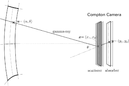
Figure 1: Compton camera.

Figure 1 schematically depicts the Compton camera system. Our target system has multiple scatterers and absorbers. A photon is detected when it is scattered at one of the scatterers and absorbed by one of the absorbers. Even if a number of photons arrive, only a little portion of them are detected after Compton scattering.

Suppose a photon from $\bm{u}=(\alpha,\delta)$ (in equatorial coordinates) is detected. It is initially scattered by one of the scatterers at $\bm{x}=(x_{1},x_{2})$ and then absorbed by one of the absorbers at $\bm{y}=(y_{1},y_{2})$. We denote the distance between the scatterer and the absorber as $d$.

Let $E_{1}$ and $E_{2}$ be the energies of the recoil electron and the scattered photon, respectively. The scattering angle $\theta$ is denoted as

$$\cos\theta=1-m_{e}c^{2}\left(\frac{1}{E_{2}}-\frac{1}{E_{1}+E_{2}}\right),$$ (1)

where $m_{e}$ and $c$ are the mass of an electron and the speed of light, respectively. The goal of Compton camera imaging is to reconstruct the gamma-ray intensity map on the celestial sphere from collected information. Difficulties arise because only the scattering angle $\theta$ is computed from a single event.

In this paper, we assume the distance from each gamma-ray source to the Compton camera system is sufficiently large. This assumption is valid for astronomy applications. Under this assumption, only the direction of arrival is important, therefore, not $\bm{x}$ and $\bm{y}$, but only the relative position normalized by the distance $d$, i.e., $\bm{w}=(\bm{x}-\bm{y})/d$, is considered. The information of each detected photon is summarized into $\bm{v}=(\bm{w},\cos\theta)$. Furthermore $\bm{u}=(\alpha,\delta)$ and $\bm{v}$ are assumed to be quantized into bins. Below, $\bm{u}$ and $\bm{v}$ are bin indices.

2.2 Compton camera measurement process

We first introduce the model of the measurement process [24]. When a gamma-ray photon from $\bm{u}$ is detected, it falls into a bin $\bm{v}$ with some probability. Let $\lambda(\bm{u})$ be the intensity of the gamma rays at pixel $\bm{u}$ of the celestial sphere and $Y(\bm{v})$ be the number of photons detected at bin $\bm{v}$ for a time interval. The distribution of $Y(\bm{v})$ follows a Poisson distribution as

$$Y(\bm{v})\sim\mathrm{Poisson}\left(\sum_{\bm{u}}t({\bm{v}},\bm{u})~{}\lambda(\bm{u})\ \right).$$ (2)

where $t({\bm{v}},\bm{u})$ is the probability that a photon from $\bm{u}$ is absorbed at $\bm{v}$. We modify the above framework in this work. Let us re-parameterize $t({\bm{v}},\bm{u})$ and $\lambda(\bm{u})$ and define $q(\bm{v})$ as follows

$$\begin{split}p({\bm{v}}\,|\,\bm{u})&=\frac{t({\bm{v}},\bm{u})}{s(\bm{u})}~{}~{}~{}{\mathrm{where}}~{}~{}~{}s(\bm{u})=\sum_{\bm{v}}t({\bm{v}},\bm{u}),\\ \rho(\bm{u})&=\frac{\lambda(\bm{u})s(\bm{u})}{\lambda}~{}~{}~{}{\mathrm{where}}~{}~{}~{}\lambda=\sum_{\bm{u}}\lambda(\bm{u})s(\bm{u})\\ q(\bm{v})&=\sum_{\bm{u}}p({\bm{v}}\,|\,\bm{u})\,\rho(\bm{u}),\end{split}$$ (3)

where $s(\bm{u})$ is the probability that a photon from pixel $\bm{u}$ is absorbed by the camera. All $\rho(\bm{u})$, $p(\bm{v}\,|\,\bm{u})$, and $q(\bm{v})$ are multinomial distributions (i.e., they are non-negative and each distribution sums up to one) conditional to the events that a photon is absorbed by the camera. More precisely, $\rho(\bm{u})$ is the probability that an absorbed photon arrives from $\bm{u}$, $p({\bm{v}}\,|\,\bm{u})$ is the probability that an absorbed photon from $\bm{u}$ is detected at $\bm{v}$, and $q(\bm{v})$ is the probability that an absorbed photon is detected at $\bm{v}$. After observing many photons, we collect information of $q(\bm{v})$. If $p(\bm{v}\,|\,\bm{u})$ is known, it is possible to estimate $\rho(\bm{u})$.

The goal of Compton camera imaging is to reconstruct the intensity map $\lambda(\bm{u})$. The distribution $\rho(\bm{u})$ differs from $\lambda(\bm{u})$ because the photons which were not completely absorbed are not included. However $\lambda(\bm{u})$ can be easily reconstructed as $\lambda(\bm{u})\propto{\rho(\bm{u})}/{s(\bm{u})}$ assuming $s(\bm{u})$ is known. Thus, we set our goal to estimate $\rho(\bm{u})$ from absorbed photons.

In the next section, we first show how to prepare $p(\bm{v}\,|\,\bm{u})$ and $s(\bm{u})$, then explain how to estimate $\rho(\bm{u})$ from absorbed photons.

3 BME methods

3.1 Bin mode

Our formulation is based on the BME, where each $\bm{v}$ and $\bm{u}$ is quantized into bins. The key is how to implement and prepare $p(\bm{v}\,|\,\bm{u})$.

If $\bm{x}$, $\bm{y}$, $E_{1}$, and $E_{2}$ are quantized separately, the number of the bins is too large and the BME is not feasible with current computational hardware. However, under the assumption that the distances from the gamma ray sources are large, it is sufficient to quantify $(\bm{w},\cos\theta)$, where $\bm{w}=(\bm{x}-\bm{y})/d$ and $\cos\theta$ are defined in eq. (1). The number of bins decreases and the BME becomes feasible without loss to precision. In previous works of COMPTEL, the matrix size was further reduced using geometrical symmetries [1, 3] but we do not rely on symmetry because the installed camera may have an asymmetric configuration.

The next challenge is how to prepare $p(\bm{v}\,|\,\bm{u})$ and $s(\bm{u})$. Here we utilize a numerical method. A Compton camera system was simulated and a lot of photons were randomly drawn numerically using software such as Geant4. The results were accumulated to compute $p(\bm{v}\,|\,\bm{u})$ and $s(\bm{u})$. This method is general and easily implemented.

There are other possible methods to compute $p(\bm{v}\,|\,\bm{u})$ and $s(\bm{u})$. One of them is to used the numerical integration based on a physical model with the Klein-Nishina formula. Although the integration is difficult, the resulting distribution is theoretically accurate. Another method is to use a physical system. When a system is built and tested under a physical environment, the collected data from a set of well-designed experiments can be used to compute $p(\bm{v}\,|\,\bm{u})$ and $s(\bm{u})$.

3.2 Maximum likelihood estimate

Next, we discuss the estimation of $\rho(\bm{u})$.

Suppose $N$ photons are detected independently and $t$-th photon is absorbed at $\bm{v}_{t}$, $(t=1,\cdots,N)$. The log likelihood function is defined as follows

$$L(\rho)=\sum_{t=1}^{N}\log\,q(\bm{v}_{t})=\sum_{t=1}^{N}\log\sum_{\bm{u}}p(\bm{v}_{t}\,|\,\bm{u})~{}\rho(\bm{u}).$$ (4)

Our goal is to estimate $\rho(\bm{u})$ from $\{\bm{v}_{t}\}$, where $p(\bm{v}\,|\,\bm{u})$ is known. The maximum likelihood estimate (MLE) of $\rho(\bm{u})$ is defined as the distribution $\rho(\bm{u})$ that maximizes $L(\rho)$. We denote it as $\hat{\rho}_{\mathrm{MLE}}(\bm{u})$. The EM algorithm [19] is a simple algorithm to compute MLE by alternately repeating the expectation (E-) step and maximization (M-) step. Each step is defined as

$$(\mbox{E-step}) q^{(l)}(\bm{v})=\sum_{\bm{u}}p(\bm{v}\,|\,\bm{u})~{}\rho^{(l)}(\bm{u}),$$ (5)

$$(\mbox{M-step}) \rho^{(l+1)}(\bm{u})=\frac{1}{N}\sum_{t=1}^{N}\frac{p(\bm{v}_{t}\,|\,\bm{u})}{q^{(l)}(\bm{v}_{t})}~{}\rho^{(l)}(\bm{u}),$$ (6)

where $l$ starts from $0$ and increases by 1 at each iteration. This algorithm can be found in a literature [25]. The log-likelihood is non-decreasing at each update, that is, $L(\rho^{(l+1)})\geq L(\rho^{(l)})$. When the difference between $q^{(l+1)}(\bm{v})$ and $q^{(l)}(\bm{v})$ becomes sufficiently small, the update is terminated. In order to measure the difference, we employed the Kullback-Leibler (KL) divergence which is defined as follows,

$$KL(q^{(l+1)},q^{(l)})=\sum_{\bm{v}}q^{(l+1)}(\bm{v})\log\frac{q^{(l+1)}(\bm{v})}{q^{(l)}(\bm{v})}.$$

Note that the KL divergence is non-negative and becomes 0 if and only if $q^{(l+1)}(\bm{v})=q^{(l)}(\bm{v})$ for all $\bm{v}$. We stopped the algorithm when $KL(q^{(l+1)},q^{(l)})$ is less than $1.0\times 10^{-10}$. The reconstructed image is proportional to the intensity map $\lambda(\bm{u})$, which is recovered from $\hat{\rho}_{\mathrm{MLE}}(\bm{u})$ as $\hat{\rho}_{\mathrm{MLE}}(\bm{u})/s(\bm{u})$.

3.3 Acceleration of the EM algorithm

The convergence speed of the EM algorithm is generally slow. In this work, we implemented an acceleration algorithm which approximates the Fisher’s scoring method [20, 21]. The Fisher’s method is a second order method, similar to the Newton’s method, and a faster convergence is expected. The proposed acceleration method was combined with a line search algorithm as in COMPTEL [3].

We show the outline of the acceleration algorithm [20, 21]. When $\rho^{(l+1)}(\bm{u})$ is computed from $\rho^{(l)}(\bm{u})$ with one EM-step, $q^{(l+1)}(\bm{v})$ is computed from eq. (5). Then another EM-step is run from $\rho^{(l)}(\bm{u})$ where $q^{(l+1)}(\bm{v})$ is the target distribution. After this EM-step, a new parameter ${\rho^{\prime}}(\bm{u})$ is obtained, which differs from $\rho^{(l+1)}(\bm{u})$ and the following parameter is computed

$$\rho^{new}(\bm{u})\propto\frac{\rho^{(l+1)}(\bm{u})^{2}}{\rho^{\prime}(\bm{u})}.$$ (7)

In most cases $L(\rho^{new}(\bm{u}))$ is larger than $L(\rho^{(l+1)}(\bm{u}))$ and the EM algorithm is accelerated [20].

The convergence speeds of the proposed acceleration method and the original EM algorithm are compared through numerical simulations in section 4.2.

3.4 Maximum a posteriori estimate

Starting from a strictly positive initial distribution $\rho^{(0)}(\bm{u})>0$, every component of $\hat{\rho}_{\mathrm{MLE}}(\bm{u})$ is strictly positive by definition. However, for astronomy applications, it is natural to assume there are a lot of $0$ components. To estimate such a sparse solution, we used the maximum a posteriori (MAP) estimation, which is a common approach in Bayesian statistics [22, 23].

Setting the prior of $\rho$ as $\pi(\rho)$, the MAP estimation maximizes the posterior probability $P(\rho,|\,\bm{v}_{1},\cdots,\bm{v}_{N})$, which is proportional to $\pi(\rho)\prod_{t}q(\bm{v}_{t})$. That is,

$$\begin{split}\hat{\rho}_{\mathrm{MAP}}&=\arg\max_{\rho}\,\Bigl{[}\,\log\,P(\rho\,|\,\bm{v}_{1},\cdots,\bm{v}_{N})\,\Bigr{]}\\ &=\arg\max_{\rho}\,\Bigl{[}\,\log\,\pi(\rho)+L(\rho)\Bigr{]},\end{split}$$ (8)

The Dirichlet distribution is the conjugate prior of a multinomial distribution [22, 23] and is often used as the prior for multinomial distributions. We use the following symmetric Dirichlet distribution with a single parameter $\beta$ as the prior of $\rho(\bm{u})$,

$$\pi_{\beta}(\rho)=\frac{\Gamma(M\beta)}{\Gamma(\beta)^{M}}\prod_{\bm{u}}\rho(\bm{u})^{\beta-1},$$ (9)

where $M$ is the number of bins of $\bm{u}$ and $\beta>0$. With this prior, eq. (8) is rewritten as $\hat{\rho}_{\mathrm{MAP}}=\arg\max_{\rho}\,\Bigl{[}\,(\beta-1)\sum_{\bm{u}}\log\,\rho(\bm{u})+L(\rho)\,\Bigr{]}$. Note that as the number of the samples increases, the log likelihood function defined in eq. (4) increases, and the influence of the prior becomes relatively small. In the limit $N\to\infty$, the MAP estimate becomes identical to the MLE.

The EM algorithm can be used to compute the MAP estimate by modifying the M-step as

$$(\mbox{M-step}) \rho^{(l+1)}(\bm{u})\propto\max\,\biggl{[}0,~{}\Bigl{(}\beta-1+\sum_{t=1}^{N}\frac{p(\bm{v}_{t}\,|\,\bm{u})}{q^{(l)}(\bm{v}_{t})}~{}\rho^{(l)}(\bm{u})\Bigr{)}\biggr{]}.$$ (10)

If $\beta=1$, the prior is uniform and the MAP estimation is identical to the MLE. However, if $\beta<1$, $\hat{\rho}_{\mathrm{MAP}}(\bm{u})$ has 0 components. The number of 0 components tends to increase as $\beta$ decreases. Although the prior in eq. (9) is improper for $\beta\leq 0$, the updating rule in eq. (10) is still valid. In the rest of the paper, we set $\beta=0$. It should be noted that the convergence speed of the above modified EM algorithm is generally faster than the original EM algorithm. The MAP estimates are computed quickly if many components of $\rho(\bm{u})$ are 0. We show some numerical results in the next section.

We proposed the MAP estimation in order to promote some components to be 0, in other word, to have a sparse solution. One concern is that some weak, possibly distributed gamma-ray sources may be neglected by the MAP estimation. When the number of received photons is small, this may be true but the influence of the prior becomes smaller as the number of absorbed photons increases. If a sufficiently large number of photons are received, the MAP reconstruction is almost identical to the MLE reconstruction and any weak sources would not be neglected.

4 Numerical Results

4.1 Simulated Compton camera

A Compton camera, which consists of 25 Si pixel detectors as the scatterers and 25 CdTe pixel detectors as the absorbers, was simulated for the numerical experiments (fig. 2). The size of each detector was identical: 100$\,\mathrm{mm}$ square and 1.0$\,\mathrm{mm}$ thick. All of the detectors were stacked in 2$\,\mathrm{mm}$ intervals. Each detector was pixellated into $50\times 50$ channels, and was assumed to have an energy resolution of $\sqrt{(2\mathrm{keV})^{2}+E^{2}}$ (full width at half maximum, FWHM), where $E$ denotes the energy deposited in the detector.

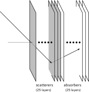
Figure 2: Simulated Compton camera with 25 layered scatterers (Si) and absorbers (CdTe). Each detector is 1.0$\,\mathrm{mm}$ thick with a 2$\,\mathrm{mm}$ separation.

In order to perform Monte Carlo simulation, a model of the Compton camera has been constructed. We used our Compton camera response generator [26], which was implemented using the Geant4 toolkit (Version 9.6.p01) [27] on a desktop computer (Mac Pro 6-core Intel Xeon 3.33 GHz). The simulations accurately treated the Doppler broadening effect of Compton scattering [28] due to the non-zero momentum of the target electron, which degrades the angular resolutions of the Compton camera. Using this simulation framework, we estimated the angular resolution measure (ARM) of the simulated Compton camera at 2.6 degrees (FWHM) for a photon energy of 661.7 keV. The ARM is defined as the difference between the reconstructed scattering angle and the actual source direction [10, 11].

In the current simulation, the range of $\alpha$ and $\delta$ were restricted between $\pm 30^{\circ}$. It is possible to widen these ranges, but the goal of this work is to build effective estimation methods. Thus, we stayed within $\pm 30^{\circ}$. In a real system, events from outside the field of view can be discarded by physical shielding and/or background rejection techniques based on Compton camera analysis prior to image reconstruction.

Table 1: Design of bins of $\bm{u}$ and $\bm{v}$.

	$\bm{u}$[degree]		$\bm{v}$
	$\alpha$	$\delta$	$\displaystyle\frac{w_{1}}{\sqrt{\,|w_{1}|\,}}$	$\displaystyle\frac{w_{2}}{\sqrt{\,|w_{2}|\,}}$	$\cos\theta$
min	$-30$	$-30$	$-2.0$	$-2.0$	$-0.56$
max	$30$	$30$	$2.0$	$2.0$	$0.96$
$\#$ of bins	$47$	$47$	$21$	$21$	$32$

The designs of image and data space is summarized in table 1. Angles $\alpha$, $\delta$, and $\cos\theta$ were quantized into equally spaced bins. For relative positions $w_{1}$ and $w_{2}$, equal spacing is not preferable because more photons are absorbed at the center than the boundaries. To prevent such unbalanced measurements, the square roots of $w_{1}$ and $w_{2}$ were quantized into equally spaced bins. The number of photons absorbed at each bin became similar under this quantization. The total numbers of bins of $\bm{u}$ and $\bm{v}$ were $47\times 47=2209$ and $21\times 21\times 32=14,112$, respectively. Each image bin was set to half of the ARM FWHM. The data space binning was also roughly optimized by evaluating the angular broadening of a point source reconstruction.

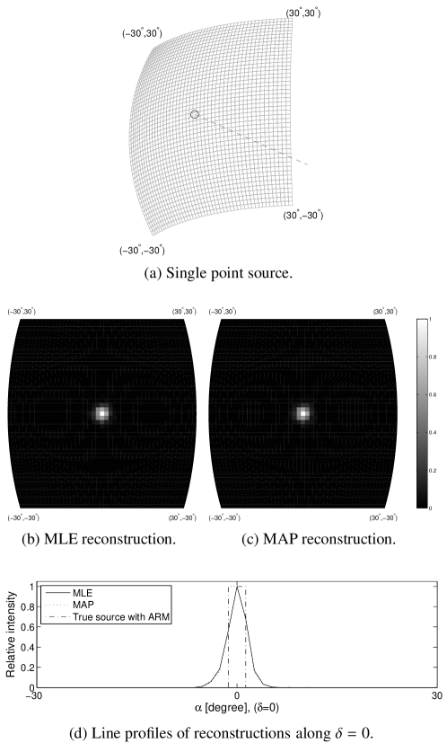
Figure 3: Gamma-ray source and estimation results. (a) Single point source. Circle indicates the position of a point source at $(0^{\circ},0^{\circ})$. Dashed line indicates the direction of the Compton camera. (b) MLE reconstruction, (c) MAP reconstruction (98 pixels are positive), and (d) line-profiles of images in (b) and (c) compared with the true source profile. Each image was normalized to have $1$ as its maximum.

In order to compute $p(\bm{v}\,|\,\bm{u})$ and $s(\bm{u})$, a large number of photons, $2.4\times 10^{10}$, were randomly generated and recorded. Total computational time for this simulation was 270 hours using an Apple Mac Pro 6-core Xeon 3.33 GHz (12 processes with hyper-threading). The energy of a gamma-ray photon was set to 661.7 keV (${}^{137}\mathrm{Cs}$). The number of detected photons was 28,817,844, which was around 0.120$\,\%$ of the total photons. The distributions $p(\bm{v}\,|\,\bm{u})$ and $s(\bm{u})$ were computed with these photon counts. It should be noted that the estimated $p(\bm{v}\,|\,\bm{u})$ had some 0’s, which could make the EM algorithm unstable. We replaced $0$’s with a small constant, $1.0\times 10^{-10}$.

This simulation only considered ${}^{137}\mathrm{Cs}$. In order to apply this method for different energy levels, $p_{E}(\bm{v}\,|\,\bm{u})$ and $s_{E}(\bm{u})$ must be prepared for each energy level $E$, and the gamma ray intensities must be estimated separately depending on the energy level $E=E_{1}+E_{2}$.

4.2 Computational times for different algorithms

We used a simple point source example in fig. 3 (a) to test the estimation algorithms. The number of simulated photons was 30,000,000 and only 108,557 photons were absorbed. We reconstructed the gamma-ray source from the detected photons.

Three algorithms were tested: the EM algorithm for the MLE, the accelerated EM algorithm for the MLE, and the modified EM algorithm for the MAP estimation. Table 2 shows the computational times and iteration numbers for convergence.

Table 2: Computational times and iteration numbers fir the three algorithms implemented on a desktop computer (Intel Core i7-3770S, 3.10 GHz) with Matlab 2013a (Ubuntu Linux 13.04, x86-64).

	time [s]	iterations
EM (MLE)	370	1563
accelerated EM (MLE)	133	514
modified EM (MAP)	7.5	755

Figure 3 shows the results. The reconstructed images of the two MLE algorithms are identical to fig. 3 (b), and the MAP reconstruction is very similar (fig. 3 (c)). However, the MAP reconstruction has only 98 positive pixels, while 2209 ($=47\times 47$) pixels are positive for the MLE reconstruction. The profiles of reconstructed images (figs. 3 (b) and (c)) along the line $\delta=0$ are shown in fig. 3 (d). It is difficult to distinguish between MLE and MAP reconstructions. The vertical bar in fig. 3 (d) indicates the location of the true source point. The width of the bar is equal to the ARM. Proposed methods provided good estimates of the true source location, and the positive regions of the reconstructed images were similar to the ARM width.

We have shown that the accelerated EM algorithm converged faster than the original EM algorithm. Moreover, the MAP estimation was very fast, and converged to a reasonable sparse image.

4.3 Image reconstruction

We next prepared four types of gamma-ray sources for numerical simulations. Sources A, B and C were two point sources (figs. 4a, 4b and 4c, respectively), and source D was a distributed source on a ring-shaped region (fig. 4d).

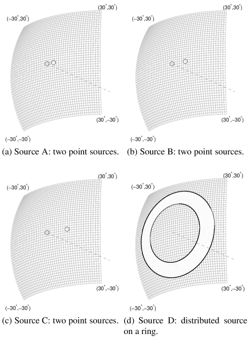
Figure 4: Gamma-ray sources used for numerical simulations: (a) source A: the circles indicate the positions of point sources at $(0^{\circ},0^{\circ})$ and $(4^{\circ},0^{\circ})$. (b) source B: two point sources at $(0^{\circ},0^{\circ})$ and $(8^{\circ},0^{\circ})$, (c) source C: two point sources at $(0^{\circ},0^{\circ})$ and $(12^{\circ},0^{\circ})$, and (d) source D: distributed source on a ring, where the outer and inner circles were $16^{\circ}$ and $24^{\circ}$ apart from the center, respectively. Dashed lines indicate the direction of the Compton camera.

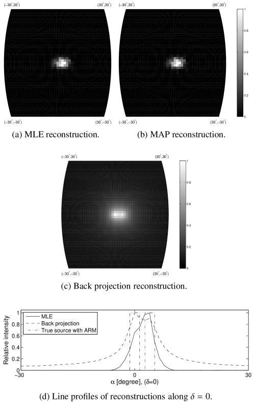
Figure 5: Reconstructed images for source A in fig. 4a. using 108,557 absorbed photons. (a) MLE reconstruction, (b) MAP reconstruction (127 pixels are positive), (c) image reconstruction with back projection, and (d) line-profiles of images in (a) and (c) compared with the true source profile. Each image was normalized to have $1$ as its maximum.

From each source model, a number of photons were randomly generated, and images were reconstructed. We compared the results of the MLE computed by the accelerated EM algorithm, the MAP estimation with the Dirichlet prior distribution ($\beta=0$), and the back-projection.

Figure 5 shows the reconstructed images for source A. The reconstructed images of the BME methods have compact positive regions but two point sources are not separated (figs. 5 (a), (b) and (d)). The back-projection reconstruction is rather diffused, but it has two peaks corresponding to the two point sources (figs. 5 (c) and (d)). Though the MLE and MAP reconstructions looks similar, each pixel of the MLE reconstruction is strictly positive whereas the MAP reconstruction has only 127 positive pixels.

Figures 6 and 7 show reconstructed images for sources B and C, respectively. For these sources, the MLE and the MAP reconstructions separate two points clearly. The line profiles show that the positive regions of the BME images are similar to the true sources with the ARM width.

Figure 8 shows the results for source D. The BME methods and back-projection clearly differ; the ring-shapes of the images recovered by the BME methods are clear and similar to the true distributed source in fig. 5 (d), while the inside of the ring of the back-projection image is positive. This is clearly seen from fig. 5 (e). The MAP estimate has only 668 positive pixels, which is around 30% of the total number of pixels.

All of the BME methods were implemented on a desktop computer (Intel Core i7-3770S, 3.10 GHz) with Matlab 2013a (Ubuntu Linux 13.04, x86-64). Table 3 summarizes the computational time and the number of iterations until convergence. The MAP estimates can be computed faster than the MLE, but the difference becomes smaller for a distributed source.

Table 3: Computational time and iteration numbers of the four simulated sources in fig. 4: the accelerated EM algorithm for the MLE and the modified EM algorithm for the MAP.

	MLE		MAP
source	time [sec]	iterations	time [sec]	iterations
A	$3.2\times 10^{2}$	770	27	1642
B	$2.6\times 10^{2}$	586	40	2103
C	$1.2\times 10^{2}$	274	32	1554
D	$2.5\times 10^{3}$	3121	$1.7\times 10^{3}$	13152

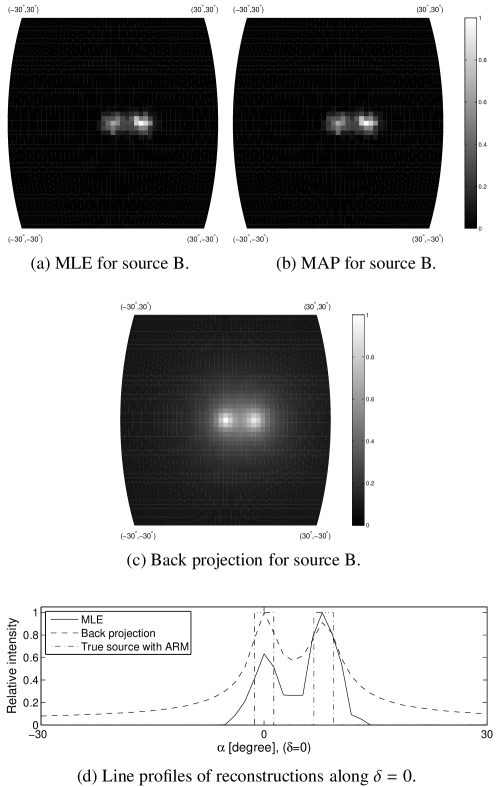
Figure 6: Reconstructed images for two point sources B in figs. 4b where 147,515 photons were absorbed. (a) MLE reconstructions, (b) MAP reconstructions (137 pixels were positive), (c) image reconstruction with the back projection, and (d) line-profiles of images in (a) and (c) compared with the true source profile. Each image was normalized to have $1$ as its maximum.

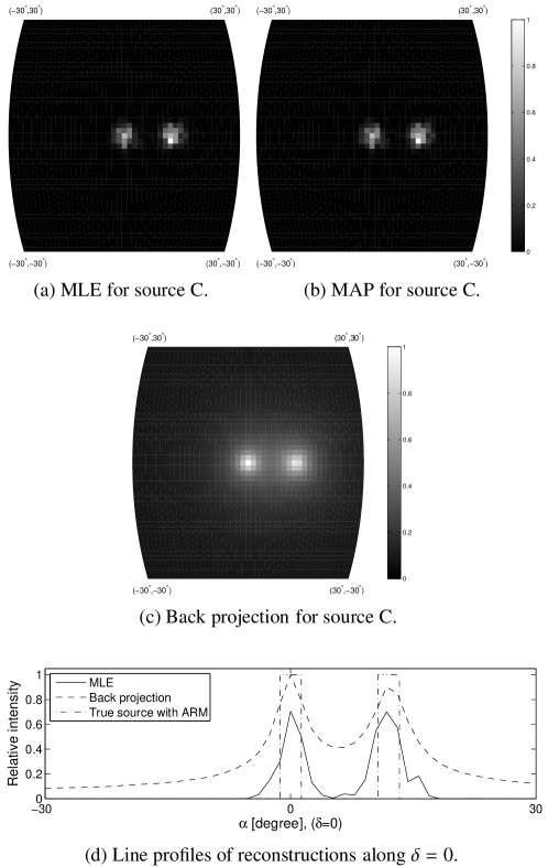
Figure 7: Reconstructed images for two point sources C in figs. 4c where 150,449 photons were absorbed. (a) MLE reconstructions, (b) MAP reconstructions (134 pixels were positive), (c) image reconstruction with the back projection, and (d) line-profiles of images in (a) and (c) compared with the true source profile. Each image was normalized to have $1$ as its maximum.

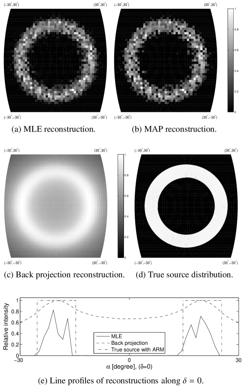
Figure 8: Reconstructed images for source D in fig. 4d where 4,337,897 photons were absorbed. (a) MLE reconstruction, (b) MAP reconstruction (668 pixels are positive), (c) image reconstruction with the back projection, and (d) true distributed gamma-ray source shown comparison. (e) line-profiles of images in (a) and (c) compared with the true source profile. Each image was normalized to have $1$ as its maximum

4.4 Discussion

Numerical results of the image reconstructions were shown in previous subsections. We provide some discussions in this subsection.

Firstly, we explain why we set the parameter $\beta$ to $0$ for the MAP estimation. Dirichlet prior with $\beta=1$ corresponds to the MLE, and the solution becomes sparser as $\beta$ decreases. Since the Bayesian prior becomes improper for $\beta\leq 0$, it is not preferable to use negative $\beta$. From the experimental results, the MAP reconstructed images of the MAP estimation with $\beta=0$ were almost identical to those of the MLE. We did not show any results for $0<\beta<1$ because the images were almost identical, and the results were less sparse. Thus, $\beta$ was set to $0$ throughout our experiments.

Secondly, we consider the convergence speed. Every BME methods was implemented with an iterative method. Therefore, the convergence speed is characterized with the computational time of one iteration and the number of iterations until the convergence. One iteration of the accelerated EM algorithm takes more time than the original EM because it uses a line search algorithm. One iteration of the MAP estimation is computed faster than the original EM. This is because the MAP estimate is sparse. The E-step shown in eq. (5) is merely a multiplication of a matrix and a vector, and if the vector is sparse, it can be computed quickly. This is why the MAP converged faster than the MLE (accelerated EM) even if the number of iterations was larger than the MLE. However, this effect becomes less evident when the reconstruction is not sparse. We see that the difference of the computational time was smaller for source (D). This is because the final reconstructed image was not sparse.

Thirdly, we discuss the source distribution. We have shown numerical results for point sources and a ring source. However, it is known that there is background emission in astronomy. The proposed method can be applied for the estimation of weak background emission, but a lot of photons must be collected. This requires a long time for observation and is not realistic in satellite applications. If the distribution form of the background is known, for example uniform, and there are point sources and background emission, it is possible to estimate the point sources and the level of the background by extending our framework. However, further details are beyond the scope of this paper.

Finally, we discuss the quality of the reconstructed images. The BME reconstructed images were not smooth compared to the back-projections. Although our results are less smooth, we observed from the line-profiles that our methods provided good estimates of the positive regions while the back-projection images became positive for the whole space. If we know that the true source is a collection of point sources, it might be possible to estimate their positions as the peaks of the back-projection image. However, if the source is distributed, it is difficult to estimate the region by the back-projection and the proposed BME methods will give better results.

We believe the reason our reconstructions were not smooth partially comes from the size of the simulation. By collecting more photons for $p(\bm{v}\,|\,\bm{u})$ and $s(\bm{u})$, we will have smoother results. This is one of our future works.

5 Conclusion

We have proposed BME methods for Compton camera imaging. Under the assumption that the distances from the gamma-ray sources are large, the number of bins can be reduced, making BME methods effective.

We follow the framework of COMPTEL and applied it to a layered system. Additionally, we propose two extensions of the EM algorithm: the acceleration of the EM algorithm for the MLE and the modified EM algorithm for the MAP estimation. Numerical simulations confirm that the accelerated EM algorithm converges faster than the original EM algorithm, and the MAP estimate converges quickly into a sparse image. The proposed methods are promising for astronomy applications. One of our goal is to apply the propose methods to real astronomy data.

We believe this paper provides a solid framework for the Compton camera imaging. The EM algorithm for the MLE is a basic approach and we have shown possible directions for extensions. In the current paper, we rely on the situation of the astronomy, where the gamma-ray sources are far from the camera. But if we can relax this assumption, we may be able to apply similar methods for the measurements of the distribution of ${}^{137}\mathrm{Cs}$ in the environment of Fukushima[8] and for medical applications.

References

- Bloemen and et al. [1994] H. Bloemen, et al., COMPTEL imaging of the Galactic disk and the separation of diffuse emission and point sources, Astrophys. Journal Suppl. Ser. 92 (1994) 412–423.
- Schönfelder and et al. [1996] V. Schönfelder, et al., COMPTEL overview: Achievements and expectations, Astron. Astrophys. Suppl. Ser. 120 (1996) 13–21.
- Knödlseder and et al. [1999] J. Knödlseder, et al., Image reconstruction of COMPTEL 1.8 MeV Al line data, Atron. Astrophys. 345 (1999) 813–825.
- LeBlanc and et al. [1998] J. LeBlanc, et al., C-SPRINT: a prototype Compton camera system for low energy gamma ray imaging, IEEE trans. Nucl. Sci. 45 (1998) 943–949.
- Takahashi and et al. [2003] T. Takahashi, et al., High resolution CdTe detectors for the next-generation multi-Compton gamma-ray telescope, Proc. SPIE 4851 (2003) 1228.
- Kanbach and et al. [2004] G. Kanbach, et al., The MEGA project, New Astronomy Reviews 48 (2004) 275–280.
- Boggs [2006] S. E. Boggs, The Advanced Compton Telescope mission, New Astronomy Reviews 50 (2006) 604–607.
- JAXA press release [2012] JAXA press release, http://www.jaxa.jp/press/2012/03/20120329_compton_e.html, 2012.
- Watanabe and et al. [2005] S. Watanabe, et al., A Si/CdTe semiconductor Compton camera, IEEE trans. Nucl. Sci. 52 (2005) 2045–2051.
- Takeda [2008] S. Takeda, Experimental Study of a Si/CdTe Semiconductor Compton Camera for the Next Generation of Gamma-ray Astronomy, Ph.D. thesis, The University of Tokyo, 2008.
- Takeda and et al. [2009] S. Takeda, et al., Experimental results of the gamma-ray imaging capability with a Si/CdTe semiconductor Compton camera, IEEE trans. Nucl. Sci. 56 (2009) 783–790.
- Odaka and et al. [2012] H. Odaka, et al., High-resolution Compton cameras based on Si/CdTe double-sided strip detectors, Nucl. Instr. and Meth. A 695 (2012) 179–183.
- Takahashi and et al. [2010] T. Takahashi, et al., The ASTRO-H mission, Proc. SPIE 7732 (2010) 77320Z.
- Tajima and et al. [2010] H. Tajima, et al., Soft gamma-ray detector for the ASTRO-H mission, Proc. SPIE 7732 (2010) 773216.
- Parra [2000] L. C. Parra, Reconstruction of cone-beam projections from Compton scattered data, IEEE trans. Nucl. Sci. 47 (2000) 1543–1550.
- Hirasawa and Tomitani [2002] M. Hirasawa, T. Tomitani, Image reconstruction from limited angle Compton camera data, Phys. Med. Biol. 47 (2002) 2129–2145.
- Xu and He [2006] D. Xu, Z. He, Filtered back-projection in Compton imaging with a single 3D position sensitive CdZnTe detector, IEEE trans. Nucl. Sci. 53 (2006) 2787–2796.
- Bandstra and et al. [2011] M. S. Bandstra, et al., Detection and imaging of the Crab Nebula with the nuclear Compton telescope, Astrophys. Journal 738:8 (2011) 9pp.
- Dempster et al. [1977] A. P. Dempster, N. M. Laird, D. B. Rubin, Maximum likelihood from incomplete data via the EM algorithm, J. R. Statistical Society, Series B 39 (1977) 1–38.
- Ikeda [2000] S. Ikeda, Acceleration of the EM algorithm, Systems and Computers in Japan 31 (2000) 10–18.
- McLachlan and Krishnan [2008] G. J. McLachlan, T. Krishnan, The EM Algorithm and Extensions, Wiley series in probability and statistics, John Wiley & Sons, Inc., 2nd edition, 2008.
- Bernardo and Smith [1994] J. M. Bernardo, A. F. M. Smith, Bayesian theory, Wiley series in probability and statistics, John Wiley & Sons, Inc., 1994.
- Bishop [2006] C. M. Bishop, Pattern Recognition and Machine Learning, Springer, 2006.
- Wilderman et al. [2001] S. J. Wilderman, N. H. Clinthorne, J. A. Fessler, W. L. Rogers, Improved modeling of system response in listmode EM reconstruction of Compton scatter camera images, IEEE trans. Nucl. Sci. 48 (2001) 111–116.
- Shepp and Vardi [1982] L. A. Shepp, Y. Vardi, Maximum likelihood reconstruction for emission tomography, IEEE trans. Medical Imaging MI-1 (1982) 113–122.
- Odaka and et al. [2010] H. Odaka, et al., Development of an integrated response generator for Si/CdTe semiconductor Compton cameras, Nucl. Instr. and Meth. A 624 (2010) 303–309.
- Allison and et al. [2006] J. Allison, et al., Geant4 developments and applications, IEEE trans. Nucl. Sci. 53 (2006) 270–278.
- Zoglauer and Kanbach [2003] A. Zoglauer, G. Kanbach, Doppler broadening as a lower limit to the angular resolution of next-generation Compton telescopes, Proc. SPIE (2003) 1302.