Computing Scalable Multivariate Glocal Invariants of Large  (Brain-) Graphs

Abstract

Graphs are quickly emerging as a leading abstraction for the representation of data. One important application domain originates from an emerging discipline called “connectomics”. Connectomics studies the brain as a graph; vertices correspond to neurons (or collections thereof) and edges correspond to structural or functional connections between them. To explore the variability of connectomes—to address both basic science questions regarding the structure of the brain, and medical health questions about psychiatry and neurology—one can study the topological properties of these brain-graphs. We define multivariate glocal graph invariants: these are features of the graph that capture various local and global topological properties of the graphs. We show that the collection of features can collectively be computed via a combination of daisy-chaining, sparse matrix representation and computations, and efficient approximations. Our custom open-source Python package serves as a back-end to a Web-service that we have created to enable researchers to upload graphs, and download the corresponding invariants in a number of different formats. Moreover, we built this package to support distributed processing on multicore machines. This is therefore an enabling technology for network science, lowering the barrier of entry by providing tools to biologists and analysts who otherwise lack these capabilities. As a demonstration, we run our code on 120 brain-graphs, each with approximately 16M vertices and up to 90M edges.

I Introduction

A wide range of naturally occurring phenomena can be accurately depicted as graphs. Subsequently, graph visualization and analysis is of ubiquitous interest in industry and academia alike—with many applications such as social network analysis [1], and recently, human brain mapping [2]. Functional and diffusion Magnetic Resonance Imaging (MRI) techniques have proven to be valuable tools for the creation of high-resolution brain-graphs[3], referred to as connectomes. These brain-graphs have great potential to unlock physiological, functional, and structural unknowns within the human brain; thereby advancing fields of study like psychiatry and neurology, by extracting biologically-relevant characterizations. Utilizing brain-graphs as biomarkers requires extracting information from the graphs that is potentially informative with regard to the covariates of interest. However, to date, no biomarkers have been useful for clinical diagnoses for any psychiatric disease category [4].

We hypothesize this lack of efficacy of contemporary biomarkers may be due to two factors. First, most analyses operate on region-wise graphs, rather than voxel-wise graphs, which reduces the number of vertices from $\mathcal{O}(10^{7})$ to $\mathcal{O}(10^{2})$. This is a substantial dimensionality reduction which almost certainly imposes severe biases and discards valuable information. Second, even given these relatively small graphs, the graph-derived features typically used are relatively simple properties of the graphs. The chosen features, therefore, may further discard clinically useful information. The reduction is largely due to computational reasons: computing graph features can be computationally daunting, exact computations often being super-exponential in the number of vertices. Existing frameworks such as igraph [5], networkx [6], and BCT [7] do not scale well to large graphs.

To address these computational deficiencies, we formally define multivariate glocal graph invariants. These graph-derived features capture a variety of local and global properties of the graphs. By utilizing sparse matrix representations and computations, in conjunction with certain approximations, we can daisy-chain computations to efficiently compute all of these glocal invariants on large graphs. All our code is implemented in an open-source Python package.

Additionally, we provide Web-services with both programmatic and point-and-click interfaces to enable investigators or analysts who lack graph analytics expertise or resources to benefit from graph processing.

Finally, we provide modules to build and compute invariants specifically for connectivity brain-graphs (i.e. connectomes) given fiber tractography streamline input data.

II Multivariate Invariants

Computing graph invariants provides a uniform platform upon which network connectivity across graphs of varying composition may be analyzed. Let $\mathcal{G}$ be the set of all graphs, where $G=(\mathcal{V}_{G},\mathcal{E}_{G})\in\mathcal{G}$, and $\mathcal{V}_{G}$ is the set of $n$ vertices $v$ for graph $G$, and $\mathcal{E}_{G}=\{u\sim v:u,v\in\mathcal{V}_{G}\}$ is the set of $m$ edges amongst $\mathcal{V}$. Let $A=(a_{uv})$ and $A^{\prime}=(a_{uv}^{\prime})$ correspond to the adjacency matrix representation for graphs $G$ and $G^{\prime}$, respectively; that is $a_{uv}=1$ if and only if $u\sim v\in\mathcal{E}_{G}$. Let $G,G^{\prime}\in\mathcal{G}$ be isomorphic to one another whenever $\exists$ such a $\pi:a_{uv}=a_{\pi(u)\pi(v)}^{\prime}$ for all $u,v\in\mathcal{V}$; where $\pi:\mathcal{V}\to\mathcal{V}$ is a permutation function (bijection). Let $G=\pi(G^{\prime})$ denote that $G$ and $G^{\prime}$ are isomorphic to one another. Let $l(u,v)$ be the minimum number of edges required to traverse between vertices $u,v\in\mathcal{V}$. Let the $j$-hop neighborhood of a graph $G$ around vertex $v$ be denoted by $N_{j}[v;G]$, where $N_{j}[v;G]=\{u\in\mathcal{V}:l(u,v)\leq j\}$. Let $\Omega(\mathcal{V}^{\prime})$ denote the induced subgraph of $\mathcal{V}^{\prime}\subseteq\mathcal{V}$, that is the graph containing vertices in $\mathcal{V}^{\prime}$ and all edges amongst them. Let $size(G)=m$ denote the number of edges in the graph, and let $[n]=\{1,2,\ldots,n\}$.

A global invariant is a function of a graph that is invariant to permutations, that is, $\Phi=\{\phi:\mathcal{G}\to\mathbb{R}^{d}$ s.t. $\phi(G)=\phi(G^{\prime})$ whenever $G=\pi(G^{\prime})\}$. Examples include number of vertices and edges, as well as max-degree, average path length, etc. A local (vertex-based) invariant is a function of a graph indexed by a vertex that is invariant to local permutations, $\Psi_{j}=\{\psi_{j}:\mathcal{G}\times\mathcal{V}\to\mathbb{R}^{p}$ s.t. $\psi(\Omega(N_{j}[v;G]))=\psi(\Omega(N_{j}[v;G^{\prime}]))$. For example, the degree of a vertex is a local invariant. A glocal invariant is the collection of local invariants for all vertices, $\Xi_{j}=\{\xi_{j}:\mathcal{G}\to\mathbb{R}^{d\times n}$ s.t. each $n$-dimensional vector is a local invariant as defined above$\}$. We will give several examples below. The invariants we compute are primarily selected due to their utility in revealing underlying network features [8]. They are arranged to vaguely reflect the degree of topological complexity they incorporate.

Degree Vector Deg $\in[n]^{n}$ is an $n$-dimensional vector where each element is an integer less than or equal to the number of vertices $n$. The degree of a vertex is defined as the number of edges incident to it, so we can compute Deg via a simple matrix vector multiply operation: Deg$(v,G)=A\mathbf{1}$, where $\mathbf{1}$ is an $n$-dimensional vector of ones.

Scan Statistic-$i$ Vector SS-$i$ $\in[n]^{n}$ is another $n$-dimensional vector where each element is the scan statistic of a particular vertex [8]. A vertex scan statistic counts the number of edges in the subgraph induced by its $i$-hop neighborhood: $size\left(\Omega(N_{i}[\upsilon;G])\right)$. SS-$j$ is the vector of these local invariants. These can be computed in an embarrassingly parallel fashion using only very local graph properties whenever $i$ is small enough. For the brain-graphs of interest, the graphs are sufficiently connected such that we can only efficiently compute SS-1 at this time.

Number of Local $3$-Cliques Vector NL-3 $\in[\binom{n}{3}]^{n}$ While Deg and SS-1 only consider pairwise interactions, NL-$j$ considers $j$-way interactions. NL-$j$ counts the number of $j$-cliques in which each vertex participates. Tsourakakis [9] demonstrated that an eigendecomposition of the adjacency matrix of the graph can be used to compute NL-$j$ for $j=3$ (also called triangles). This approximation, however, does not work with modification for $4$-cliques. Thus, although number of local $j$-cliques would be an interesting multivariate glocal invariant, we could not design an efficient algorithm to approximate it at this time. For NL-3 however, in experiments, we achieved 99.9% accuracy on graphs with 3,000 vertices and $\sim$4 million edges, using only 1 eigen-pair. The main computation is NL-3$(v,G)\approx\frac{1}{2}\sum_{k=1}^{K}\lambda^{3}_{k}(G)x^{2}_{vk}(G)$ where, $x_{vk}(G)$ is the $v^{th}$ entry of the $k^{th}$ eigenvector of $A$, and $\lambda_{k}(G)$ is the $k^{th}$ eigenvalue, $K$ is the number of eigen-pairs used in the approximation.

Clustering Coefficient Vector CC $\in[\binom{n}{3}]^{n}$ combines Deg and NL-3 to assess the relative amount of connectivity as compared to the potential total amount of connectivity for each vertex. To efficiently compute CC we utilize the previous computations, thus obtaining this additional glocal invariant is essentially free [10]. For each vertex, we compute $CC(v,G)=2\times NL$-$3(v,G)/({Deg(v,G)(Deg(v,G)-1)})$.

Latent Position Matrix LP-$k$ $\in\mathbb{R}^{k\times n}$ is a $k$-dimensional estimate of the latent positions of each vertex [11]. Latent position random graph models are elegant statistical models of random graphs with many desirable properties. In short, associated with each vertex is a latent position vector $x_{v}\in\mathbb{R}^{k}$, and the probability of an edge between vertex $u$ and $v$ is a function of the dissimilarity between the latent positions $\kappa(x_{u},x_{v})$. It has been shown that an eigendecomposition of the adjacency matrix of a graph yields universally consistent estimators for various parameters of a certain general class of latent position models [12]. Thus, this multivariate glocal invariant utilizes global topological properties, rather than just $j$-neighborhoods as in the previous glocal invariants. For efficiency, we calculate the first $k$ eigenvectors via the Lanczos algorithm [13]. Moreover, since we estimate NL-3 via the eigendecomposition, our NL-3 approximation becomes essentially free after computing LP-1.

Thus, the total collection of all multivariate glocal graph invariants are available after an eigendecomposition, a couple of local searches, and a few matrix vector multiply operations.

III Software Tools

We have developed novel tools to compute multivariate invariants on large scale graphs, including voxel-wise brain-graphs. The tools we have developed are designed to run on the CPU with as little as one core and a minimum of 8 GB of RAM. These software tools can be publicly accessed via a stand-alone Python Package or our Web-Services.

III-A Stand-alone Package

The package, written in Python 2.7, provides users with the ability to download, utilize and freely modify the existing implementations of invariant calculations. Additionally, we developed a set of command-line tools (CLTs), via executable scripts; these provide a high-level and simple way to safely interact with the actual data processing scripts. These CLTs are appropriate for, and have been successfully deployed [14] in, distributed environments for the parallel processing of graphs. Finally, we provide scripts to build MRI fiber streamline graphs. This requires two inputs: (i) a fiber streamline file, in MRI Studio DAT format, and (ii) a mask composed of two files that together describe the regions of interest (ROIs), in XML and RAW format. Any voxels outside these ROIs are excluded when creating graph edges.

The resulting brain-graph is stored as a sparse, compressed, and symmetric square matrix. We further elaborate on the methodology for building these connectome graphs in Section IV. This open-source package is downloadable from https://github.com/openconnectome/MR-connectome/tree/stand-alone. The distribution also includes several example scripts.

III-B Web-services

Our Web-services are accessible at http://openconnecto.me/graph-services/, run on our own data-intensive cluster. These Web-services can be invoked through a graphical user interface via web browser, or programmatically via the command line. Both modes permit multiple-subject jobs, enabling the processing of several graphs with a single action. Programmatic interface functionality is well documented on the website with several example Python scripts and command line calls to each service. The Web-services actively use our stand-alone package as the data processing back-end for graph building and invariant calculations. Available Web-services include:

(i) computing invariants on dense or compressed sparse column (CSC) square matrices in MATLAB (MAT) format, (ii) conversion of invariant and graph files between MAT, NPY and CSV formats, and (iii) building connectome graphs from diffusion MRI data.

IV Experiments

To demonstrate how our software can be used, we programmatically computed the invariants of 120 subjects’ connectome graphs using our Web-services (see Figure 1).

IV-A Computational Methodology

To generate the brain-graphs, we begin with derivative data in the form of fiber tractography streamlines and a mask. These fiber streamlines, and the mask are by-products of MIGRAINE, a pipeline for efficiently computing large brain-graphs from raw multimodal magnetic resonance imaging data [14]. MIGRAINE ingests the raw structural and diffusion MRI scans. The mask—which may describe ROIs, brain masks or grey matter—is applied to the data to exclude voxels outside the masked region from the brain-graph. Based on fiber tracing, we allocate edges to each pair of remaining voxels that are connected by fibers. The count of fibers between a pair of connected voxels yields a weight for each graph edge. These edge weights are later thresholded and binarized because we compute only unweighted invariants.

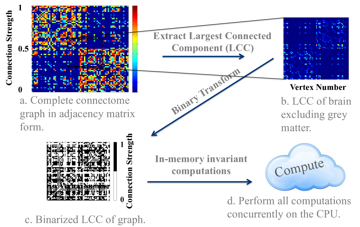
Figure 1: Pipeline showing data transformation phases where we extract the LCC prior to brain-graph binarization and invariant computation.

As depicted in Figure 1 we extract a subset of the full brain-graph by taking the Largest Connected Component (LCC) [15]. Our implementation includes a flag that enables operating on the LCC for the following reasons:

• The LCC is by definition a connected graph, thus eigenvector embeddings of it are especially interesting due to their theoretical properties [16], [17].

• The LCC is of particular interest in many applications—thus computed invariants on the LCC are useful to a wide variety of researchers [18].

• The LCC discards isolates and other vertices that are potentially “noisy”. Graph size is reduced from $O(10^{7})$ to $(10^{5})$ vertices while graph order is marginally affected with $>$99% of edges remaining. This substantially decreases processing time by 94% to under 2 hours per graph.

IV-B Results

By extrapolating the measured empirical accuracy of smaller graphs, we estimate that given 100 eigen-pairs, the NL-3 algorithm has an accuracy of nearly 94% on graphs of the LCC containing $O(10^{5})$ vertices and $O(10^{7})$ edges. Note that Deg and SS-1 are unaffected by the number of eigen-pairs, whereas NL-3 and subsequently CC are affected. Figure 2 depicts all invariants computed on all subjects, with color indicating gender. This is an example of how our tools might be used: the invariants may be used as features to discover individual brain differences as a function of phenotype, including psychiatric diagnosis and aptitude.

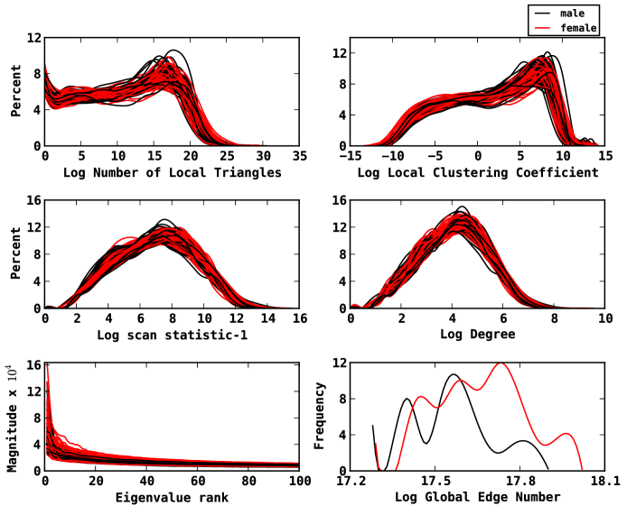
Figure 2: Multivariate invariants of 120 subjects superimposed over one another.

V Computing Performance

To quantify performance we averaged measures such as I/O rates, RAM/CPU usage, for the 120 graphs that we processed (Figure 2). One of the goals of the computational package is that it be compatible with hardware constraints of modern laptops. Thus, we performed all experiments on a single core, never exceeding 6.5 GB of RAM usage (see Figure 3).

For computational efficiency, our implementations are a close-knit merger and coalesced series of invariants. For example, our CC estimate uses our NL-3 estimate which uses our eigendecomposition. Thus, we compute the collection of multivariate glocal invariants both daisy-chaining appropriate functions and performing each independently. To facilitate benchmarking against other graph processing packages, Table I depicts the computational load for each invariant.

Total compute time for all invariants is $\sim$2.9 hour per graph, per core, when computed separately. Note that we include the time taken to compute the invariant in addition to any prerequisite computations necessary. Total compute time upon appropriately daisy-chaining is $\sim$1.8 h per graph, per core, a speedup of approximately $60\%$.

TABLE I: Analysis of algorithms used and experimental time (mean and standard deviation per vertex per core) using a single 4 core, 2.4 GHz processor Linux server with 16 GB of ram.

Invariant	Time Complexity	Wall Time
Clustering Coefficient	$O(n+k)$	$0.59$ $(\pm 2.4)$ $\mu$s
Number of Local 3-Cliques	$O(n+k)$	$48.51$ $(\pm 0.9)$ $\mu$s
Degree	$O(n)$	$66.64$ $(\pm 1.8)$ $\mu$s
Scan Statistic-1	$O(nm)$	$0.47$ $(\pm 0.2)$ $m$s
Latent Position-100	$O(100(m+n))$	$45.41$ $(\pm 0.1)$ $\mu$s

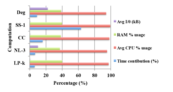
Figure 3: Performance of each invariant, computed serially and independently of any non-dependent invariants on an 4 core, 2.4 GHz processor Linux server with 16 GB of RAM.

VI Future Work

We have already incorporated some of this functionality into igraph [5] and MIGRAINE [14], with plans to also incorporate it into neuroimaging specific packages such as the Configurable Pipeline for the Analysis of Connectomes (CPAC) [19].

Moreover, we will extend the back-end to take advantage of faster/multithreaded eigensolvers, including GPU implementations. In order to maximize utility to researchers, we will continue to develop our software suite by computing other network-elucidating invariants such as Scan Statistic-2 [8], graph diameter, clique number, and more. Finally, we will utilize these invariants to develop biomarkers for a variety of neuropsychiatric and psychological conditions [4].

VII Acknowledgments

This work was supported by the following institutions and grants: The National Institutes of Health (NIBIB 1RO1EB016411-01), The National Science Foundation (OCI-1244820), The Office of Naval Research, and The Johns Hopkins University, Institute for Data Intensive Engineering and Science.

References

- [1] Bhaumik, C., Agrawal, A. K., and Sinha, P. Using social network graphs for search space reduction in internet of things. In Proceedings of the 2012 ACM Conference on Ubiquitous Computing - UbiComp ’12, 602 (ACM Press, New York, New York, USA, 2012).
- [2] Craddock, R. C., Jbabdi, S., Yan, C.-G., Vogelstein, J. T., Castellanos, F. X., Di Martino, A., Kelly, C., Heberlein, K., Colcombe, S., and Milham, M. P. Imaging human connectomes at the macroscale. Nature methods10(6), 524–39 June (2013).
- [3] Hagmann, P., Cammoun, L., Gigandet, X., Meuli, R., Honey, C. J., Wedeen, V. J., and Sporns, O. Mapping the structural core of human cerebral cortex. PLoS biology6(7), e159 July (2008).
- [4] First, M. B., Botteron, K. N., Castellanos, X. F., Dickstein, D. P., Drevets, W. C., Kim, K. L., Pescosolido, M. F., Rausch, S., Seymour, K. E., Sheline, Y. I., and Zubieta, J.-K. Consensus Report of the APA Working Group on Neuroimaging Markers of Psychiatric Disorders. Technical report, (2012).
- [5] Csardi, G. and Nepusz, T. The igraph Software Package for Complex Network Research. InterJournalComplex Sy (2006).
- [6] Hagberg, A., Swart, P., and S Chult, D. Exploring network structure, dynamics, and function using networkx. SCIPY 08 January (2008).
- [7] Rubinov, M. and Sporns, O. Complex network measures of brain connectivity: uses and interpretations. NeuroImage52(3), 1059–69 September (2010).
- [8] Pao, H., Coppersmith, G. a., and Priebe, C. E. Statistical Inference on Random Graphs: Comparative Power Analyses via Monte Carlo. Journal of Computational and Graphical Statistics20(2), 395–416 January (2011).
- [9] Tsourakakis, C. Fast Counting of Triangles in Large Real Networks: Algorithms and Laws. In cis.temple.edu, 608–617 (Data Mining, 2008. ICDM ’08. Eighth IEEE International Conference, Pisa, 2008).
- [10] Saramäki, J., Kivelä, M., Onnela, J.-P., Kaski, K., and Kertész, J. Generalizations of the clustering coefficient to weighted complex networks. Physical Review E75(2), 027105 February (2007).
- [11] Hoff, P. D., Raftery, A. E., and Handcock, M. S. Latent Space Approaches to Social Network Analysis. Journal of the American Statistical Association97(460), 1090–1098 December (2002).
- [12] Sussman, D. L., Tang, M., and Priebe, C. E. Universally Consistent Latent Position Estimation and Vertex Classification for Random Dot Product Graphs. arXiv preprint 1212.1182.
- [13] Lanczos, C. An iteration method for the solution of the eigenvalue problem of linear differential and integral operators. Journal of Research of the National Bureau of Standards45(4), 255 October (1950).
- [14] Gray, R. W., Koterba, Z. H., Mhembere, D., Kleissas, D. M., Vogelstein, J. T., Burns, R., and Vogelstein, R. J. MRI Graph Analysis and Inference for Connectomics ( MIGRAINE ). (Accepted) (2013).
- [15] Jones, E., Oliphant, T., Peterson, P., and Al, E. Scipy: Open source scientific tools for Python, (2001).
- [16] Sussman, D. L., Tang, M., and Priebe, C. E. Universally Consistent Latent Position Estimation and Vertex Classification for Random Dot Product Graphs. arXiv preprint arXiv:1212.1182 July (2012).
- [17] Fishkind, D. E., Sussman, D. L., Tang, M., Vogelstein, J. T., and Priebe, C. E. Consistent adjacency-spectral partitioning for the stochastic block model when the model parameters are unknown. Journal of the American Statistical Association107, 1119–1128 May (2012).
- [18] Zalesky, A., Solowij, N., Yücel, M., Lubman, D. I., Takagi, M., Harding, I. H., Lorenzetti, V., Wang, R., Searle, K., Pantelis, C., and Seal, M. Effect of long-term cannabis use on axonal fibre connectivity. Brain : a journal of neurology135(Pt 7), 2245–55 July (2012).
- [19] Sikka, S., Vogelstein, J. T., and Milham, M. P. Towards Automated Analysis of Connectomes: The Configurable Pipeline for the Analysis of Connectomes (C-PAC). In Organization of Human Brain Mapping. Neuroinformatics, (2012).