Small Universal Petri Nets with Inhibitor Arcs

Abstract.

We investigate the problem of construction of small-size universal Petri nets with inhibitor arcs. We consider four descriptional complexity parameters: the number of places, transitions, inhibitor arcs, and the maximal degree of a transition, each of which we try to minimize. We give six constructions having the following values of parameters (listed in the above order): $(30,34,13,3)$, $(14,31,51,8)$, $(11,31,79,11)$, $(21,25,13,5)$, $(67,64,8,3)$, $(58,55,8,5)$ that improve the few known results on this topic. Our investigation also highlights several interesting trade-offs.

1. Introduction

The concept of universality was first formulated by A. Turing in [15]. He constructed a universal (Turing) machine capable of simulating the computation of any other (Turing) machine. This universal machine takes as input a description of the machine to simulate, the contents of its input tape, and computes the result of its execution on the given input. The universal Turing machine is extremely important as it provided the first theoretical basis for the construction of modern computers – this becomes obvious if we consider the latter as fixed universal devices which receive as input the coding of the algorithm solving a problem (the program) and the input data, and which produce the result of the execution of the algorithm (program) on that input data.

More generally, the universality problem for a class of computing devices (or functions) $\mathfrak{C}$ consists in finding a fixed element $\mathcal{M}$ of $\mathfrak{C}$ able to simulate the computation of any element $\mathcal{M}^{\prime}$ of $\mathfrak{C}$ using an appropriate fixed encoding. More precisely, if $\mathcal{M}^{\prime}$ computes $y$ on an input $x$ (we will write this as $\mathcal{M}^{\prime}(x)=y$), then $\mathcal{M}^{\prime}(x)=f(\mathcal{M}(g(\mathcal{M}^{\prime}),h(x)))$, where $h$ and $f$ are the encoding and decoding functions, respectively, and $g$ is the function retrieving the number of $\mathcal{M}^{\prime}$ in some fixed enumeration of $\mathfrak{C}$. These functions should not be too complicated, otherwise the universal machine will be trivial, e.g. when $f$ is partially recursive the machine can contain only one instruction – stop. It is commonly admitted that general recursive functions can be used for encoding and decoding. The typically used functions are $f(x)=\log_{2}(x)$ and $h(x)=2^{x}$. The element $\mathcal{M}$ is called (weakly) universal for $\mathfrak{C}$. We shall call $\mathcal{M}$ strongly universal (for $\mathfrak{C}$) if the encoding and decoding functions are identities.

Some authors [5, 4] implicitly consider only the strong notion of universality as the encoding and decoding functions can perform quite complicated transformations, which are not necessarily doable in the original devices. For example, Minsky’s proof of (weak) universality of register machines with two counters [7] makes use of exponential (resp. logarithmic) encoding (resp. decoding) functions, while it is known that such functions cannot be computed on these machines [2]. We refer to [4] for a more detailed discussion of different variants of the universality. Generally, the class of all partially recursive functions is considered as $\mathfrak{C}$, but it is possible to have a narrower class, e.g. the class of all primitive recursive functions, which is known to admit a universal generally recursive function [5].

In 1956 Shannon [14] considered the question of finding the smallest possible universal Turing machine where the size is calculated as the number of states and symbols. In the early sixties, Minsky and Watanabe had a running competition to see who could find the smallest universal Turing machine [6, 17]. Later, Rogozhin showed the construction of several small universal Turing machines [12]. An overview of recent results on this topic can be found in [8]. Other computational models were also considered, e.g. cellular automata [16] with a construction of universal cellular automata of rather small size; see [9, 18] for an overview.

Small universal devices have mostly theoretical importance as they demonstrate the minimal ingredients needed to achieve a complex (universal) computation. Their construction is a long-standing and fascinating challenge involving a lot of interconnections between different models, constructions, and encodings.

Turing machines and cellular automata work on strings and, in order to represent functions, unary encoding is used. Register machines [7] manipulate numbers directly and it was shown that three registers are sufficient for strong universality. However, corresponding constructions are quite big as far as the number of used rules is concerned. In 1996, Korec constructed several small universal register machines [4] that made use of a reduced number of rules. These results served as the base for the universal constructions for multiset rewriting-based models (which are equivalent to vector addition systems and Petri nets). In [1] a small universal maximally parallel multiset rewriting system is constructed. Due to equivalences between Petri nets and multiset rewriting systems, this result can be seen as a universal Petri net working with max step semantics. For the traditional class of Petri nets there were no known universality constructions for a long time. Recently, Zaitsev has investigated the universality of Petri nets with inhibitor arcs and priorities [20] and has constructed a small universal net with 14 places and 29 transitions (for nets without priorities the same author obtained a universal net with 500 places and 500 transitions [19]). We remark that inhibitor arcs and priorities are equivalent extensions for Petri nets in terms of computational power, so using both concepts together is not necessary for universality constructions.

In this article, we perform a systematic investigation of Petri nets with inhibitor arcs working in the classical sequential semantics. We consider as a measure of descriptional complexity the vector $(p,t,h,d)$, where $p$ is the number of places, $t$ is the number of transitions, $h$ is the number of inhibitor arcs, and $d$ is the maximal degree of a transition. We remark that from the multiset rewriting point of view these parameters correspond to the size of the alphabet, the number of rules, the number of forbidding conditions and the maximal size of the rule, respectively. We construct strongly universal deterministic Petri nets with inhibitor arcs of the following sizes: $(30,34,13,3)$, $(14,31,51,8)$, $(11,31,79,11)$, $(21,25,13,5)$, $(67,64,8,3)$, $(58,55,8,5)$. The obtained results highlight several trade-offs between the parameters, e.g. the construction from Section 6 shows how the decrease in the number of inhibitor arcs translates to the increase of the number of places and transitions, while that in Section 4 decreases the number of states by incrementing the number of the inhibitor arcs and the degree of the transitions.

2. Preliminaries

In this section we recall some basic notions and notations used in formal language theory, and computability theory that we will need in the rest of the paper. For further details and information the reader is referred to [13].

An alphabet is a finite non-empty set of symbols. Given an alphabet $V$, we designate by $V^{*}$ the set of all strings over $V$, including the empty string, $\lambda$. For each $x\in V^{*}$ and $a\in V$, $|x|_{a}$ denotes the number of occurrences of the symbol $a$ in $x$. A finite multiset over $V$ is a mapping $X:V\longrightarrow\mathbb{N}$, where $\mathbb{N}$ denotes the set of non-negative integers. $X(a)$ is said to be the multiplicity of $a$ in $X$.

2.1. Register machines

A deterministic register machine is defined as a 5-tuple $M=(Q,R,q_{0},q_{f},P),$ where $Q$ is a set of states, $R=\{R_{1},\dots,R_{k}\}$ is the set of registers, $q_{0}\in Q$ is the initial state, $q_{f}\in Q$ is the final state and $P$ is a set of instructions (called also rules) of the following form:

1. (Increment) $(p,RiP,q)\in P$, $p,q\in Q,p\neq q,R_{i}\in R$ (being in state $p$, increment register $R_{i}$ and go to state $q$).

2. (Decrement) $(p,RiM,q)\in P$, $p,q\in Q,p\neq q,R_{i}\in R$ (being in state $p$, decrement register $R_{i}$ and go to state $q$).

3. (Zero check) $(p,Ri,q,s)\in P$, $p,q,s\in Q,R_{i}\in R$ (being in state $p$, go to $q$ if register $R_{i}$ is not zero or to $s$ otherwise).

4. (Zero test and decrement) $(p,RiZM,q,s)\in P$, $p,q,s\in Q,R_{i}\in R$ (being in state $p$, decrement register $R_{i}$ and go to $q$ if successful or to $s$ otherwise).

5. (Stop) $(q_{f},STOP)$ (may be associated only to the final state $q_{f}$).

We note that for each state $p$ there is only one instruction of the types above.

For conciseness, we will often refer to a rule of type $(q_{j},X,q_{k})$ or eventually $(q_{j},X,q_{k},q_{k^{\prime}})$, just by the symbol $X$.

A configuration of a register machine is given by the $(k+1)$-tuple $(q,n_{1},\dots,n_{k})$, where $q\in Q$ and $n_{i}\in\mathbb{N},1\leq i\leq k$, describing the current state of the machine as well as the contents of all registers. A transition of the register machine consists in updating/checking the value of a register according to an instruction of one of the types above and in changing the current state to another one. We say that the machine stops if it reaches the state $q_{f}$. We say that $M$ computes a value $y\in\mathbb{N}$ on the input $x_{1},\dots,x_{n}$, $x_{i}\in\mathbb{N}$, $1\leq i\leq n\leq k$, if, starting from the initial configuration $(q_{0},x_{1},\dots,x_{n},0,\dots,0)$, it reaches the final configuration $(q_{f},y,0,\dots,0)$.

It is well-known that register machines compute all partial recursive functions and only them [7]. Therefore, every register machine $M$ with $n$ registers can be associated with the function it computes: an $m$-ary partial recursive function $\Phi_{M}^{m}$, where $m\leq n$. Let $\Phi_{0},\Phi_{1},\Phi_{2},\dots,$ be a fixed enumeration of the set of unary partial recursive functions. Then, a register machine $M$ is said to be strongly universal if there exists a recursive function $g$ such that $\Phi_{x}(y)=\Phi_{M}^{2}(g(x),y)$ holds for all $x,y\in\mathbb{N}$. A register machine $M$ is said to be (weakly) universal if there exist recursive functions $f,g,h$ such that $\Phi_{x}(y)=f(\Phi_{M}^{2}(g(x),h(y)))$ holds for all $x,y\in\mathbb{N}$.

We also note that the power and efficiency of a register machine $M$ depend on the set of used instructions. In [4] several sets of instructions are investigated. In particular, it is shown that there are strongly universal register machines with 22 instructions of form $RiP$ and $RiZM$. Moreover, these machines can be effectively constructed.

Figure 1 shows this universal register machine having 22 instructions of type $RiP$ and $RiZM$ taken from [4] (more precisely in [4] only a machine with 32 instructions of type $RiP$, $RiM$ and $Ri$ is constructed, and the machine below may be easily obtained from that one by combining the instructions of type $Ri$ and $RiM$).

Figure 1. Flowchart of the strongly universal machine $U_{22}$.

Here is the list of rules of this machine:

$$\begin{array}[]{llll}(q_{1},R1ZM,q_{3},q_{6})&(q_{3},R7P,q_{1}){}&(q_{4},R5ZM,q_{6},q_{7})\\ (q_{6},R6P,q_{4}){}&(q_{7},R6ZM,q_{9},q_{4})&(q_{9},R5P,q_{10}){}\\ (q_{10},R7ZM,q_{12},q_{13})&(q_{12},R1P,q_{7}){}&(q_{13},R6ZM,q_{33},q_{1})\\ (q_{33},R6P,q_{14}){}&(q_{14},R4ZM,q_{1},q_{16})&(q_{16},R5ZM,q_{18},q_{23})\\ (q_{18},R5ZM,q_{20},q_{27})&(q_{20},R5ZM,q_{22},q_{30})&(q_{22},R4P,q_{16}){}\\ (q_{23},R2ZM,q_{32},q_{25})&(q_{25},R0ZM,q_{1},q_{32})&(q_{27},R3ZM,q_{32},q_{1})\\ (q_{29},R0P,q_{1}){}&(q_{30},R2P,q_{31}){}&(q_{31},R3P,q_{32}){}\\ (q_{32},R4ZM,q_{1},q_{f})&(q_{f},STOP)\end{array}$$

For the purposes of this paper, we will prefer a different representation of register machines as graphs, the one in which the graph vertices carry only the information about the states, while the operations and conditions are attached to the arcs. Figure 4a shows such a representation of the segment of $U_{22}$ centered at the states $q_{10}$ and $q_{13}$. We use the symbols $Ri$ (resp. $RiZ$) to describe the conditions in which the register $R_{i}$ is required to be nonzero (resp. zero), while the symbols $RiP$ and $RiM$ stand for the operations of incrementing and decrementing $R_{i}$. Such a construct is more general than a register machine, because more than one operation or condition may be attached to arcs. We will later see how this generality contributes to the minimisation of universal Petri nets.

2.2. Petri Nets

A Place-Transition-net or for short, PT-net, with inhibitor arcs is a construct $N=(P,T,W,M_{0})$ where $P$ is a finite set of places, $T$ is a finite set of transitions, with $P\cap T=\emptyset$, $W:(P\times T)\cup(T\times P)\to\mathbb{N}\cup\{-1\}$ is the weight function and $M_{0}$ is a multiset over $P$ called the initial marking.

PT-nets are usually represented by diagrams where places are drawn as circles, transitions are drawn as squares annotated with their location, and a directed arc $(x,y)$ is added between $x$ and $y$ if $W(x,y)\geq 1$. These arcs are then annotated with their weight if this one is $2$ or more. Arcs having the weight -1 are called inhibitor arcs and are drawn such that the arcs end with a small circle on the side of the transition.

Given a PT-net $N$, the pre- and post-multiset of a transition $t$ are respectively the multiset $pre_{N(t)}$ and the multiset $post_{N(t)}$ such that, for all $p\in P$, for which $W(p,t)\geq 0$, $pre_{N(t)}(p)=W(p,t)$ and $post_{N(t)}(p)=W(t,p)$. A state of $N$, which is called a marking, is a multiset $M$ over $P$; in particular, for every $p\in P$, $M(p)$ represents the number of tokens present inside place $p$. A transition $t$ is enabled at a marking $M$ if the multiset $pre_{N(t)}$ is contained in the multiset $M$ and all inhibitor places $p$ (such that $W(p,t)=-1$) are empty. An enabled transition $t$ at marking $M$ can fire and produce a new marking $M^{\prime}$ such that $M^{\prime}=M-pre_{N(t)}+post_{N(t)}$ (i.e., for every place $p\in P$, the firing transition $t$ consumes $pre_{N(t)}(p)$ tokens and produces $post_{N(t)}(p)$ tokens). We denote this as $M\overset{t}{\longrightarrow}M^{\prime}$.

For the purposes of this paper, we have to define which kind of PT-nets can execute computations (e.g. compute partially recursive functions). In such a net some distinguished places $i_{1},\dots,i_{k}$, $k>0$ from $P$ are called input places (which are normally different from the places marked in $M_{0}$ containing the control tokens) and one other, $i_{0}\in P$, is called the output place. The computation of the net $N$ on the input vector $(n_{1},\dots,n_{k})$ starts with the initial marking $M_{0}^{\prime}$ such that $M_{0}^{\prime}(i_{j})=n_{j}$ and $M_{0}^{\prime}(x)=M_{0}(x),$ for all $x\neq i_{j}$, $1\leq j\leq k$. This net will evolve by firing transitions until deadlock in some marking $M_{f}$, i.e. in $M_{f}$ no transition is enabled. Thus we have $M_{0}^{\prime}\overset{*}{\longrightarrow}M_{f}$ and there are no $M_{f}^{\prime}$ and $t\in T$ such that $M_{f}\overset{t}{\longrightarrow}M_{f}^{\prime}$. The result of the computation of $N$ on the vector $(n_{1},\dots,n_{k})$, denoted by $\Phi_{N}^{k}(n_{1},\dots,n_{k})$, is defined as $M_{f}(i_{0})$, i.e. the number of tokens in place $(i_{0})$ in the final state. Since in the general case Petri nets are non-deterministic, the function $\Phi_{N}^{k}$ could compute a set of numbers. In this paper we consider only those nets, which compute a unique result and which are deterministic, that is, for any reachable marking $M$, there is at most one marking $M^{\prime}$ such that $M\to M^{\prime}$. This corresponds to labelled deterministic Petri nets in which all transitions are labelled with the same symbol [10].

3. Universal Net with Small Transition Degree

In this section we will show how to construct a universal Petri net with transitions of degree of most 3, based on the universal register machine $U_{22}$ shown in Subsection 2.1. We will then evaluate some basic parameters of the obtained Petri net: the number of places, the number of transitions, the number of inhibitor arcs, and the maximal degree of a transition.

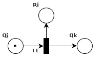
(a) a

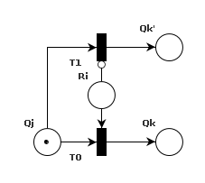
(b) b

Figure 2. Petri nets simulating instructions of type $RiP$ and $RiZM$.

In $U_{22}$, only rules of type $RiZM$, and $RiP$ are used. We will now show how these types of rules can be implemented in Petri nets. The general idea is to have one place $Qj$ for each state $q_{j}$ and one place $Ri$ per register $R_{i}$. A token in place $Qj$ means that the simulated machine is in state $q_{j}$, while the number of tokens in place $Ri$ corresponds to the value of the register $R_{i}$ of the simulated machine.

A Petri net simulating an instruction of type $RiP$ is shown in Figure 2a. It is rather clear that the only transition of this Petri net correctly moves the state token from the $Qj$ to $Qk$ and adds one to the value of the register $Ri$.

A Petri net simulating an instruction of type $RiZM$ is shown in Figure 2b. There are two transitions going out of $Qj$: one moves the token from $Qj$ into $Qk$ and can only be fired when $Ri$ contains at least one token so that we can decrement its value. The other transition on the contrary can only be fired when $Ri$ contains no tokens and moves the token from $Qj$ to $Qk^{\prime}$.

We can now directly construct the universal Petri net simulating the register machine $U_{22}$ by iteratively translating all instructions. For reasons of readability, we will refrain from showing the resulting universal Petri net. At the initial marking this net will have one token in place $Q1$ corresponding to state $q_{1}$ of $U_{22}$. This Petri net has 22 places for states and 8 places for registers, 30 states all in all. There are 34 transitions in this net, as many as there are arcs in the graph representation of $U_{22}$. Further, the number of inhibitor arcs in this Petri net equals to the number of $RiZM$ instructions in the simulated register machine: 13. Finally, since we only simulate rules of type $RiP$ and $RiZM$, the maximal transition degree is 3. Obviously, with such an approach, this is the absolute minimal value, because there must be transitions which move the state token between two state places and also modify a register place. Therefore, the descriptional complexity of this net is $(30,34,13,3)$. We will refer to this net as $N_{1}$.

We remark that register machine $U_{22}$ supposes that the code of the machine to be simulated is initially placed in register $R_{1}$ and the initial value in register $R_{2}$. Under these conditions the result can be read in register $R_{0}$ when the machine halts. Hence, $N_{1}$ has two input places $R1$ and $R2$ and an output place $R0$. Now in order to simulate an arbitrary Petri net $N$ with one input place, $N_{1}$ shall be provided by the appropriate coding of $N$ and its input in places $R1$ and $R2$ respectively. The net $N_{1}$ is strongly universal because of the relation $\Phi_{N}(x)=\Phi^{2}_{N_{1}}(g(N),x)$, where $g$ is an enumeration function. We remark that if we would like to obtain the complete final marking of $N$ as a result, then this could be done by constructing another net $N^{\prime}$ which additionally encodes the final configuration of $N$ into a number and then using a decoding function to transform it to a vector.

4. Universal Nets with a Small Number of Places

In this section we construct two universal Petri nets with inhibitor arcs where we focus on reducing the number of places. This reduction can be achieved using two independent ideas: (a) performing several register machine instructions in one Petri net transition and (b) using a binary encoding of the states. In both cases the states corresponding to the states of the register machine are reduced; in case (a) unused states are eliminated, in case (b) their number becomes logarithmic with respect to the initial amount.

4.1. State Compression

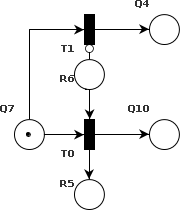
Figure 3. A Petri net simulating the states $q_{7}$ and $q_{9}$ of $U_{22}$.

The main idea behind this optimization is that, in Petri nets, more than one register machine operation can be performed in one transition. For example, the sequence of operations performed in states $q_{7}$ and $q_{9}$ can be implemented in Petri nets as shown if Figure 3. Generally, we can save one place on a $RiP$ instruction by carrying the corresponding increment of the register in the preceding transition.

Moreover, it is possible to save a state place on two successive $RiZM$ instructions. Consider the situation depicted in Figure 4a. Instead of directly translating these two instructions into Petri nets using the patterns we have seen in the previous section, we will merge the two potential transitions into one and thus save a state place, as shown in Figure 4b.

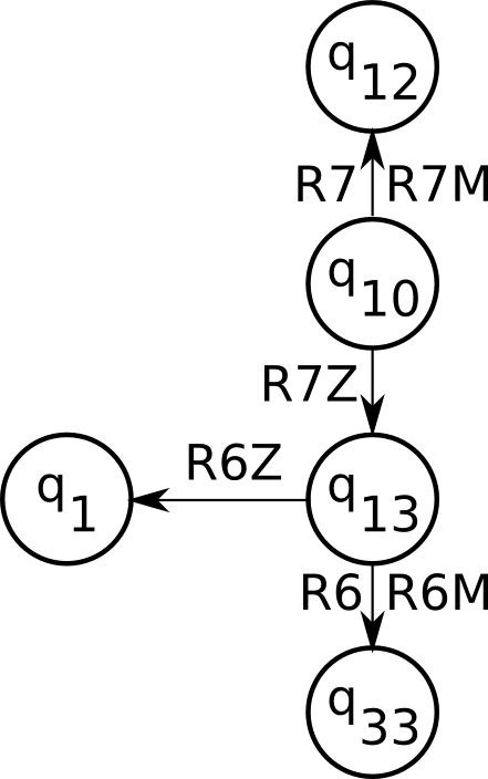
(a) a

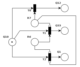
(b) a

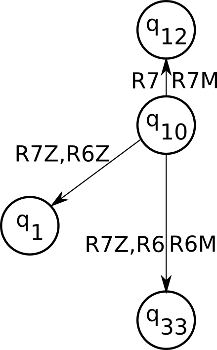
(c) a

Figure 4. The translation of successive $RiZM$ and $RjZM$ instructions to Petri nets.

The central question now is when such an optimization technique cannot be applied. The answer arises from the semantics of Petri net transitions: before a transition is fired, the conditions are checked whether it can be fired or not. Therefore, in a single Petri net transition, checking a condition on a register can only be performed before the value of this register is modified.

Note that using a $RiZM$ instruction to check the value of a register immediately after it was modified by a $RiP$ instruction is redundant because we know for sure that the register is not zero. This allows us to state that, in a single transition, we can perform any series of actions which do not include decrements of the register $R_{i}$ and then check its value.

We can now turn back to graphs of register machines and formulate the algorithm of reducing (compressing) the number of states. We first define the notion of a compressible state: a state $q$ is compressible if (a) no arc leaving $q$ checks a register modified by an $RiM$ instruction of an incoming arc, and (b) if $q$ has no loop arcs (i.e., arcs which do not move the machine away from state $q$). Reducing a compressible state $q$ is generally done in the following way: for every pair of states $q_{pred}$ and $q_{succ}$ for which there exist the arcs $q_{pred}\to q$ and $q\to q_{succ}$, we add a new arc $q_{pred}\to q_{succ}$ which combines the conditions and operations of these two arcs. We then remove the state $q$ and all associated arcs.

An important remark is due here: if the arc $q_{pred}\to q$ increments a register that is subsequently required to be nonzero by the arc $q\to q_{succ}$, then we have to remove the (redundant) check from the conditions of the new arc $q_{pred}\to q_{succ}$. If, on the other hand, this register is required to be zero, we just do not add the arc $q_{pred}\to q_{succ}$ altogether, because such a state transition is impossible.

We also need to carefully handle the cases in which the incoming and the outgoing arcs impose conditions on the same register. Consider, for example, a compressible state $q_{k}$, an arc $q_{j}\to q_{k}$ which requires $R_{i}$ to be zero, and then another arc $q_{k}\to q_{m}$, which, as well, requires $R_{i}$ to be zero. The new arc $q_{j}\to q_{m}$ can only be added in case $q_{j}\to q_{k}$ does not increment $R_{i}$, because, obviously, the condition that $R_{i}$ should be zero imposed by $q_{k}\to q_{m}$ is rendered impossible. Generally, the following four scenarios have to be kept in mind:

1. both $q_{pred}\to q$ and $q\to q_{succ}$ require $R_{i}$ to be zero,

2. $q_{pred}\to q$ requires $R_{i}$ to be zero, while $q\to q_{succ}$ requires it to be nonzero,

3. $q_{pred}\to q$ requires $R_{i}$ to be nonzero, while $q\to q_{succ}$ requires it to be zero, and

4. both $q_{pred}\to q$ and $q\to q_{succ}$ require $R_{i}$ to be nonzero.

In the first situation we can only construct the new arc $q_{pred}\to q_{succ}$ if $q_{pred}\to q$ does not increment $R_{i}$. In the second case, we can only add the new arc if $q_{pred}\to q$ does increment $R_{i}$. In the third case we can never add a new transition because, if $R_{i}$ is not decremented, then it cannot become zero and the conditions of $q\to q_{succ}$ cannot be satisfied. On the other hand, if $q_{pred}\to q$ decrements $R_{i}$, $q$ would not be compressible. Finally, in the fourth case, we should always add the new transition because, by the supposition that $q$ is compressible, we know that $q_{pred}\to q$ does not decrement $R_{i}$ and there is no chance that it becomes empty.

Now, the state reduction algorithm is defined as iterative reduction of compressible states. Using this algorithm, it is possible to compress the graph corresponding to the original register machine $U_{22}$ to a construct with 7 states, including a $STOP$ state. We will refer to this construct as $\mathcal{U}_{7}$; the program of $\mathcal{U}_{7}$ can be found in the appendix. The Petri net associated with $\mathcal{U}_{7}$ has 14 places, 31 transitions, 51 inhibitor arcs, and the maximal transition degree equal to 8; the descriptional complexity of this net is therefore $(14,31,51,8)$. At the initial marking, the place $Q3$, obtained by compression of state $q_{3}$, will contain one token. We will refer to this net as $N_{2}$.

4.2. Binary Coding of State Numbers

We can further reduce the number of places of the universal Petri net by avoiding the allocation of a place per state, but instead coding the current state number in binary. If the simulated register machine has $n$ states, we will use $\lceil\log_{2}n\rceil=n_{p}$ places to codify the current state number in the following way: the place $Qi$, $0\leq i<n_{p}$, contains a token if the $i$-th bit of the binary representation of $n$ is one, and is empty otherwise. All transitions of such a Petri net will thus depend on all the state places $Qi$, $0\leq i<n_{p}$, and will produce the new marking of the state places corresponding to the next state number.

As an example, consider the following instruction of an imaginary register machine with 8 states: $(q_{4},R0P,q_{6})$. This instruction defines one transition going out of the state $q_{4}$ and into state $q_{6}$; we will need $\lceil\log_{2}8\rceil=3$ state places to simulate this register machine. Supposing that the numbering of states is zero-based, the binary code for state $q_{4}$ will be $(100)_{2}$, and $(110)_{2}$ for $q_{6}$. Therefore we can draw the Petri net simulating this transition with binary-coded state numbers as shown in Figure 5.

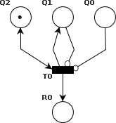
Figure 5. A Petri net simulating a $RiP$ instructions with binary coded states.

The transition can only be fired when $Q2$ contains at least a token, and $Q1$ and $Q0$ are empty, which corresponds to the binary number $(100)_{2}$ and to state $q_{4}$. The effect of this transition is adding a token to the register place $R0$, leaving the token of $Q2$ in place, putting a token into $Q1$, and leaving $Q0$ empty. The marking of the state places $Q2$, $Q1$, and $Q0$ after the firing of this transition corresponds to the binary number $(110)_{2}$ and to state $q_{6}$.

Clearly, coding states in binary can be done for any register machine. We will apply this technique to the construct $\mathcal{U}_{7}$ obtained previously. That machine had 7 states, which means that we will need 3 state places with binary coding in the associated net. This amounts to $11$ places all in all. Because of the encoding more arcs should be added to each transition and this augments the maximal transition degree to the value 11. As far as the number of inhibitor arcs is concerned, it is important to realize that this parameter will also vary depending on how exactly the states are numbered, because the number of transitions going out of each state differs. The strategy we adopt in order to keep the number of inhibitors slightly lower is to assign the greater binary number to the state with more outgoing arcs. Since checking for a zero binary digit takes an inhibitor arc, following this strategy will minimize the number of such arcs in the net. Moreover, it is possible to eliminate the STOP state by erasing corresponding incoming transitions, hence yielding the net into a deadlock (which corresponds to the halting condition for the Petri nets). The number we have obtained is 28 extra arcs for reading the binary-coded state, which gives 79 inhibitor arcs all in all, including the 51 arcs resulting from state compression.

Finally, the number of transitions of the Petri net employing this binary coding of states is the same as that of the net $N_{2}$: 31. This amounts to the following possible descriptional complexity: $(11,31,79,11)$. We will refer to this net as $N_{3}$. The construct $\mathcal{U}_{7}$ starts in state 3 which is assigned the code $(010)_{2}$, which means that, at the initial marking, $N_{3}$ will contain one token in place $Q1$.

5. Universal Net with a Small Number of Transitions

We consider the construction given in the Section 3 and we show how the number of transitions can be decreased. We use the following observation already formulated in Subsection 4.1: the increment instructions of the register machine $U_{22}$ can be simulated during previous zero check and decrement instruction, so the corresponding state can be omitted from the net, see Figure 3. Applied to the net $N_{1}$ this process eliminates 9 states and 9 transitions, yielding a new universal net $N_{4}$ having the descriptional complexity described by the vector $(21,25,13,5)$. At the initial marking, $N_{4}$ will have one token in place $Q1$ corresponding to state $q_{1}$.

6. Universal Net with a Small Number of Inhibitor Arcs

We have seen that Petri nets we have constructed so far used inhibitor arcs heavily. From the Petri nets we constructed, those having the smallest number of inhibitor arcs is $N_{1}$ with 13 inhibitor arcs. It turns out that it is possible to almost halve this parameter and reduce the number of inhibitor arcs to 8 – one per each register of the simulated register machine. The main idea is to centralize the procedure of checking whether a register is zero and to reuse the checker subnet whenever this kind of information is required.

Consider the following $RiZM$ instruction: $(q_{j},RiZM,q_{k},q_{k^{\prime}})$. Figure 6 shows a Petri net which simulates this instruction. This net works in the following way. Whenever it is required to take a decision based on the contents of the register $R_{i}$, the state token from $Qj$ is “split” into two: one token goes into the waiting place $Qj^{\prime}$ and another token goes into $C_{i}$ of the $R_{i}$ checker block (highlighted in the figure). The checker block checks the value of the register (performs the actual $RiZM$ instruction), and moves the token from $Ci$ to $CiZ$ or $CiNZ$, depending on the value of $Ri$. Whenever a token is put into $CiZ$ or $CiNZ$, either the transition $T3$ or $T4$ is activated, moving the state token into $Qk^{\prime}$ if $Ri$ is zero or into $Qk$ if the value of the register was nonzero and has thus been decremented.

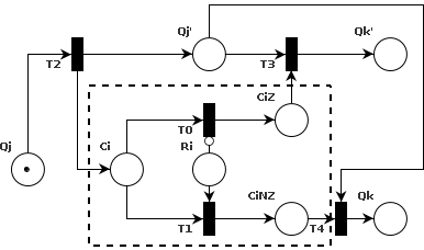
Figure 6. A Petri net simulating a $RiZM$ instruction using a checker subnet.

Clearly, the checker block can be shared across as many simulations of $RiZM$ instructions as necessary, which means that indeed the number of inhibitor arcs can be reduced to 8.

We apply the idea of register checkers to the Petri net $N_{1}$. To count the states, we note that each checker subnet contains three places plus one for the register, which makes it 32 places for registers and checkers. The simulation of a $RiZM$ requires one extra place in the model with checkers, which amounts to 13 extra places, one per each of the 13 $RiZM$ instructions. Finally, there are 22 states, which translates to 22 places. All in all, the Petri net will contain $32+13+22=67$ places.

As far as the maximal degree of a transition is concerned, note that we do not use transitions of degree greater than 3 in the simulation of any instruction. This brings focus upon the clear trade-off between the number of states and the number of inhibitor arcs.

The number of transitions of the Petri net using checker blocks can be computed as follows. Each checker block introduces two new transitions, which amounts to 16 transitions for eight checker blocks. Further, we need three transitions per each simulation of a $RiZM$ instructions, which amounts to 39 transitions for the 13 such instructions of $U_{22}$. Finally, there are 9 $RiP$ instructions and 9 Petri net transitions to simulate them. All in all, there are 64 transitions. The descriptional complexity of this net called $N_{5}$ is therefore $(67,64,8,3)$.

By attaching $RiP$ instructions to the previous decrement instructions, the number of states and transitions can be slightly decreased; the price to be paid is the increase in the maximal degree. The corresponding descriptional complexity is $(58,55,8,5)$. We will refer to this net as $N_{6}$.

Both $N_{5}$ and $N_{6}$ will contain a token in place $Q1$ at their initial markings.

7. Main Results

To summarize the results we have obtained in the paper, we formulate the following statement.

Theorem 7.1.

There exist strongly universal Petri nets of following sizes:
$(30,34,13,3)$, $(14,31,51,8)$, $(11,31,79,11)$, $(21,25,13,5)$, $(67,64,8,3)$, and $(58,55,8,5)$.

In a completely analogous way, the ideas shown previously can be applied to the weakly universal register machine $U_{20}$ from point (b2) of the Main Theorem from [4]. We thus formulate the following result.

Theorem 7.2.

There exist weakly universal Petri nets of following sizes:
$(27,31,12,3)$, $(14,21,23,8)$, $(10,21,44,10)$, $(20,24,12,5)$, $(64,60,8,3)$, and $(57,53,8,3)$.

8. Conclusion

In this paper we constructed 6 strongly universal Petri nets with inhibitor arcs with sizes shown in Theorem 7.1, trying to propose an optimal result for each parameter. While the parameters’ space is 4-dimensional, our results particularly exhibit pairwise relations between some parameters. As a future work it could be interesting to consider constructions where the trade-off between 3 or 4 parameters can be observed.

Another interesting question is the minimal value for each of the parameters. It is clear that the minimal value for the degree is equal to 3 thus we reached the lower bound in this direction. The number of needed inhibitor arcs is at least two, as nets with one arc have a decidable reachability problem [11, 3] which implies that in the computational variant the halting is decidable. Hence there cannot be universal nets with one inhibitor arc for the class of partially recursive functions. So it could be an interesting challenge to construct a small net having 2 or 3 inhibitor arcs only.

For the other parameters we cannot indicate a lower bound; we conjecture that the number of transitions cannot be below 25 (which is the number of branching points in the Korec machine). We also think that it would be difficult to substantially decrease the number of states with respect to what was obtained in the paper.

We would also like to remark that since the original register machine is deterministic and since our translations preserve this property, the resulting Petri nets are also deterministic.

Appendix A Descriptions of Some of the Constructions

In this appendix, we will give the incidence matrices of some of the universal Petri nets constructed in this paper. The columns of these tables correspond to states, the rows to transitions, and each cell of represents the pair of arc weights $W(p,t),W(t,p)$.

	Q3	Q4	Q10	Q16	Q18	Q20	R0	R1	R2	R3	R4	R5	R6	R7
T1	1,1							1,0						0,1
T2	1,0	0,1						-1,0					0,1	0,1
T3		1,1										-1,0	-1,0
T4		1,1										1,0	0,1
T5		1,0	0,1									-1,1	1,0
T6	0,1		1,0					1,0					-1,0	-1,0
T7	0,1		1,0					1,0			1,0		2,0	-1,0
T8		0,1	1,0					0,1					-1,0	1,0
T9		0,1	1,0					-1,0			1,0		2,1	-1,0
T10		0,1	1,0					-1,0					-1,1	-1,0
T11			1,1					0,1				0,1	1,0	1,0
T12			1,0	0,1							-1,0		2,0	-1,0
T13	0,1			1,0			1,0	1,0	-1,0			-1,0
T14	0,1			1,0				1,0	1,0		1,0	-1,0
T15	0,1			1,0			-1,0	1,0	-1,0		1,0	-1,0
T16		0,1		1,0			1,0	-1,0	-1,0			-1,0	0,1
T17		0,1		1,0				-1,0	1,0		1,0	-1,0	0,1
T18		0,1		1,0			-1,0	-1,0	-1,0		1,0	-1,0	0,1
T19				1,0	0,1							1,0
T20				1,0			-1,0		-1,0		-1,0	-1,0
T21				1,0					1,0		-1,0	-1,0
T22	0,1				1,0		0,1	1,0		-1,0		-1,0
T23	0,1				1,0			1,0		1,0	1,0	-1,0
T24		0,1			1,0		0,1	-1,0		-1,0		-1,0	0,1
T25		0,1			1,0			-1,0		1,0	1,0	-1,0	0,1
T26					1,0	0,1						1,0
T27					1,0					1,0	-1,0	-1,0
T28	0,1					1,0		1,0	0,1	0,1	1,0	-1,0
T29		0,1				1,0		-1,0	0,1	0,1	1,0	-1,0	0,1
T30				0,1		1,0					0,1	1,0
T31						1,0			0,1	0,1	-1,0	-1,0

Table 1. The incidence table of the Petri net $N_{2}$ of size $(14,31,51,8)$.

	Q0	Q1	Q2	R0	R1	R2	R3	R4	R5	R6	R7
T1	-1,0	1,1	-1,0		1,0						0,1
T2	-1,1	1,1	-1,0		-1,0					0,1	0,1
T3	1,1	1,1	-1,0						-1,0	-1,0
T4	1,1	1,1	-1,0						1,0	0,1
T5	1,0	1,1	-1,1						-1,1	1,0
T6	-1,0	1,1	1,0		1,0					-1,0	-1,0
T7	-1,0	1,1	1,0		1,0			1,0		2,0	-1,0
T8	-1,1	1,1	1,0		0,1					-1,0	1,0
T9	-1,1	1,1	1,0		-1,0			1,0		2,1	-1,0
T10	-1,1	1,1	1,0		-1,0					-1,1	-1,0
T11	-1,0	1,1	1,1		0,1				0,1	1,0	1,0
T12	-1,1	1,1	1,1					-1,0		2,0	-1,0
T13	1,0	1,1	1,0	1,0	1,0	-1,0			-1,0
T14	1,0	1,1	1,0		1,0	1,0		1,0	-1,0
T15	1,0	1,1	1,0	-1,0	1,0	-1,0		1,0	-1,0
T16	1,1	1,1	1,0	1,0	-1,0	-1,0			-1,0	0,1
T17	1,1	1,1	1,0		-1,0	1,0		1,0	-1,0	0,1
T18	1,1	1,1	1,0	-1,0	-1,0	-1,0		1,0	-1,0	0,1
T19	1,1	1,0	1,1						1,0
T20	1,0	1,0	1,0	-1,0		-1,0		-1,0	-1,0
T21	1,0	1,0	1,0			1,0		-1,0	-1,0
T22	1,0	-1,1	1,0	0,1	1,0		-1,0		-1,0
T23	1,0	-1,1	1,0		1,0		1,0	1,0	-1,0
T24	1,1	-1,1	1,0	0,1	-1,0		-1,0		-1,0	0,1
T25	1,1	-1,1	1,0		-1,0		1,0	1,0	-1,0	0,1
T26	1,0	-1,0	1,1						1,0
T27	1,0	-1,0	1,0				1,0	-1,0	-1,0
T28	-1,0	-1,1	1,0		1,0	0,1	0,1	1,0	-1,0
T29	-1,1	-1,1	1,0		-1,0	0,1	0,1	1,0	-1,0	0,1
T30	-1,1	-1,1	1,1					0,1	1,0
T31	-1,0	-1,0	1,0			0,1	0,1	-1,0	-1,0

Table 2. The incidence table of a Petri net $N_{3}$ of size $(11,31,79,11)$.

	Q1	Q3	Q4	Q6	Q7	Q9	Q10	Q12	Q13	Q14	Q16	Q18	Q20	Q22	Q23	Q25	Q27	Q29	Q30	Q31	Q32	Q33	R0	R1	R2	R3	R4	R5	R6	R7
T1	1,0	0,1																						1,0
T2	1,0			0,1																				-1,0
T3	0,1	1,0																												0,1
T4			1,0	0,1																								1,0
T5			1,0		0,1																							-1,0
T6			0,1	1,0																									0,1
T7			0,1		1,0																								-1,0
T8					1,0	0,1																							1,0
T9						1,0	0,1																					0,1
T10							1,0	0,1																						1,0
T11							1,0		0,1																					-1,0
T12					0,1			1,0																0,1
T13	0,1								1,0																				-1,0
T14									1,0													0,1							1,0
T15	0,1									1,0																	1,0
T16										1,0	0,1																-1,0
T17											1,0	0,1																1,0
T18											1,0				0,1													-1,0
T19												1,0	0,1															1,0
T20												1,0					0,1											-1,0
T21													1,0	0,1														1,0
T22													1,0						0,1									-1,0
T23											0,1			1,0													0,1
T24															1,0	0,1									-1,0
T25															1,0						0,1				1,0
T26	0,1															1,0							1,0
T27																1,0					0,1		-1,0
T28																	1,0	0,1								-1,0
T29																	1,0				0,1					1,0
T30	0,1																	1,0					0,1
T31																			1,0	0,1					0,1
T32																				1,0	0,1					0,1
T33	0,1																				1,0						1,0
T34										0,1												1,0							0,1

Table 3. The incidence table of the Petri net $N_{1}$ of size $(30,34,13,3)$.

	Q1	Q3	Q4	Q6	Q7	Q9	Q10	Q12	Q13	Q14	Q16	Q18	Q20	Q22	Q23	Q27	Q30	Q31	Q32	Q33	R0	R1	R2	R4	R5	R6	R7
T1	1,0	0,1																				1,0
T2	1,0			0,1																		-1,0
T3	0,1	1,0																									0,1
T4			1,0	0,1																					1,0
T5			1,0		0,1																				-1,0
T6			0,1	1,0																						0,1
T7			0,1		1,0																					-1,0
T8					1,0	0,1																				1,0
T9						1,0	0,1																		0,1
T10							1,0	0,1																			1,0
T11							1,0		0,1																		-1,0
T12					0,1			1,0														0,1
T13	0,1								1,0																	-1,0
T14									1,0											0,1						1,0
T15	0,1									1,0														1,0
T16										1,0	0,1													-1,0
T17											1,0	0,1													1,0
T18											1,0				0,1										-1,0
T19												1,0	0,1												1,0
T20												1,0				0,1									-1,0
T21													1,0	0,1											1,0
T22													1,0				0,1								-1,0
T23											0,1			1,0										0,1
T24	0,1														1,0						-1,0
T25															1,0				0,1		1,0
T26	0,1															1,0							-1,0
T27																1,0			0,1				1,0
T28																	1,0	0,1			0,1
T29																		1,0	0,1				0,1
T30	0,1																		1,0					1,0
T31										0,1										1,0						0,1

Table 4. The incidence table of the Petri net $N^{w}_{1}$ of size $(27,31,12,3)$.

	Q1	Q4	Q10	Q16	Q18	Q20	R0	R1	R2	R4	R5	R6	R7
T1	1,1							1,0					0,1
T2	1,0	0,1						-1,0				0,1
T3		1,1									-1,0	-1,0
T4		1,1									1,0	0,1
T5		1,0	0,1								-1,1	1,0
T6	0,1		1,0									-1,0	-1,0
T7	0,1		1,0							1,0		1,1	-1,0
T8		0,1	1,0					0,1				-1,0	1,0
T9			1,1					0,1			0,1	1,0	1,0
T10			1,0	0,1						-1,0		1,1	-1,0
T11	0,1			1,0			-1,0				-1,0
T12	0,1			1,0			1,0		1,0	2,0	-1,0
T13				1,0	0,1						1,0
T14				1,0			1,0			-1,0	-1,0
T15	0,1				1,0				-1,0		-1,0
T16	0,1				1,0				2,0	2,0	-1,0
T17					1,0	0,1					1,0
T18					1,0				1,0	-1,0	-1,0
T19	0,1					1,0	0,1		1,1	2,0	-1,0
T20				0,1		1,0				0,1	1,0
T21						1,0	0,1		0,1	-1,0	-1,0

Table 5. The incidence table of the Petri net $N^{w}_{2}$ of size $(14,21,23,8)$.

	Q0	Q1	Q2	R0	R1	R2	R4	R5	R6	R7
T1	-1,0	1,1	-1,0		1,0					0,1
T2	-1,0	1,0	-1,1		-1,0				0,1
T3	-1,0	-1,0	1,1					-1,0	-1,0
T4	-1,0	-1,0	1,1					1,0	0,1
T5	-1,1	-1,1	1,1					-1,1	1,0
T6	1,0	1,1	1,0						-1,0	-1,0
T7	1,0	1,1	1,0				1,0		1,1	-1,0
T8	1,0	1,0	1,1		0,1				-1,0	1,0
T9	1,1	1,1	1,1		0,1			0,1	1,0	1,0
T10	1,0	1,1	1,1				-1,0		1,1	-1,0
T11	-1,0	1,1	1,0	-1,0				-1,0
T12	-1,0	1,1	1,0	1,0		1,0	2,0	-1,0
T13	-1,1	1,0	1,1					1,0
T14	-1,0	1,0	1,0	1,0			-1,0	-1,0
T15	1,0	-1,1	1,0			-1,0		-1,0
T16	1,0	-1,1	1,0			2,0	2,0	-1,0
T17	1,1	-1,1	1,0					1,0
T18	1,0	-1,0	1,0			1,0	-1,0	-1,0
T19	1,0	1,1	-1,0	0,1		1,1	2,0	-1,0
T20	1,0	1,1	-1,1				0,1	1,0
T21	1,0	1,0	-1,0	0,1		0,1	-1,0	-1,0

Table 6. The incidence table of a Petri net $N^{w}_{3}$ of size $(10,21,44,10)$.

$q_{i}$	$q_{j}$	Conditions	Operations
1	1	$R_{1}\neq 0$	$R1M$, $R7P$
1	2	$R_{1}=0$	$R6P$, $R7P$
2	2	$R_{5}=0$, $R_{6}=0$
2	2	$R_{5}\neq 0$	$R5M$, $R6P$
2	3	$R_{5}=0$, $R_{6}\neq 0$	$R5P$, $R6M$
3	1	$R_{1}\neq 0$, $R_{6}=0$, $R_{7}=0$	$R1M$
3	1	$R_{1}\neq 0$, $R_{4}\neq 0$, $R_{6}\neq 0$, $R_{7}=0$	$R1M$, $R4M$
3	2	$R_{6}=0$, $R_{7}\neq 0$	$R1P$, $R7M$
3	2	$R_{1}=0$, $R_{4}\neq 0$, $R_{6}\neq 0$, $R_{7}=0$	$R4M$, $R6P$
3	2	$R_{1}=0$, $R_{6}=0$, $R_{7}=0$	$R6P$
3	3	$R_{6}\neq 0$, $R_{7}\neq 0$	$R1P$, $R5P$, $R6M$, $R7M$
3	4	$R_{4}=0$, $R_{6}\neq 0$, $R_{7}=0$
4	1	$R_{0}\neq 0$, $R_{1}\neq 0$, $R_{2}=0$, $R_{5}=0$	$R0M$, $R1M$
4	1	$R_{1}\neq 0$, $R_{2}\neq 0$, $R_{4}\neq 0$, $R_{5}=0$	$R1M$, $R2M$, $R4M$
4	1	$R_{0}=0$, $R_{1}\neq 0$, $R_{2}=0$, $R_{4}\neq 0$, $R_{5}=0$	$R1M$, $R4M$
4	2	$R_{0}\neq 0$, $R_{1}=0$, $R_{2}=0$, $R_{5}=0$	$R0M$, $R6P$
4	2	$R_{1}=0$, $R_{2}\neq 0$, $R_{4}\neq 0$, $R_{5}=0$	$R2M$, $R4M$, $R6P$
4	2	$R_{0}=0$, $R_{1}=0$, $R_{2}=0$, $R_{4}\neq 0$, $R_{5}=0$	$R4M$, $R6P$
4	5	$R_{5}\neq 0$	$R5M$
4	7	$R_{0}=0$, $R_{2}=0$, $R_{4}=0$, $R_{5}=0$
4	7	$R_{2}\neq 0$, $R_{4}=0$, $R_{5}=0$	$R2M$
5	1	$R_{1}\neq 0$, $R_{3}=0$, $R_{5}=0$	$R0P$, $R1M$
5	1	$R_{1}\neq 0$, $R_{3}\neq 0$, $R_{4}\neq 0$, $R_{5}=0$	$R1M$, $R3M$, $R4M$
5	2	$R_{1}=0$, $R_{3}=0$, $R_{5}=0$	$R0P$, $R6P$
5	2	$R_{1}=0$, $R_{3}\neq 0$, $R_{4}\neq 0$, $R_{5}=0$	$R3M$, $R4M$, $R6P$
5	6	$R_{5}\neq 0$	$R5M$
5	7	$R_{3}\neq 0$, $R_{4}=0$, $R_{5}=0$	$R3M$
6	1	$R_{1}\neq 0$, $R_{4}\neq 0$, $R_{5}=0$	$R1M$, $R2P$, $R3P$, $R4M$
6	2	$R_{1}=0$, $R_{4}\neq 0$, $R_{5}=0$	$R2P$, $R3P$, $R4M$, $R6P$
6	4	$R_{5}\neq 0$	$R4P$, $R5M$
6	7	$R_{4}=0$, $R_{5}=0$	$R2P$, $R3P$

Table 7. The program of the universal machine $\mathcal{U}_{7}$. Each line corresponds to a transition from state $q_{i}$ to state $q_{j}$, checking the conditions listed in the “Conditions” column and performing those operations on registers which are given in the “Operations” column.

References

- [1] Artiom Alhazov and Sergey Verlan. Minimization strategies for maximally parallel multiset rewriting systems. Theoretical Computer Science, 412(17):1581 – 1591, 2011.
- [2] Ian M. Barzdin. Ob odnom klasse machin Turinga (machiny Minskogo), russian. Algebra i Logika, 1:42–51, 1963.
- [3] Hans Kleine Büning, Theodor Lettmann, and Ernst W. Mayr. Projections of vector addition system reachability sets are semilinear. Theoretical Computer Science, 64(3):343–350, 1989.
- [4] Ivan Korec. Small universal register machines. Theoretical Computer Science, 168(2):267–301, 1996.
- [5] Anatoly I. Malcev. Algorithms and Recursive Functions. Groningen, Wolters-Noordhoff Pub. Co., 1970.
- [6] Marvin Minsky. Size and structure of universal Turing machines using tag systems. In Recursive Function Theory: Proceedings, Symposium in Pure Mathematics, Provelence, volume 5, pages 229–238, 1962.
- [7] Marvin Minsky. Computations: Finite and Infinite Machines. Prentice Hall, Englewood Cliffts, NJ, 1967.
- [8] Turlough Neary and Damien Woods. The complexity of small universal Turing machines: A survey. In Mária Bieliková, Gerhard Friedrich, Georg Gottlob, Stefan Katzenbeisser, and György Turán, editors, SOFSEM 2012: 38th Conference on Current Trends in Theory and Practice of Computer Science, volume 7147 of Lecture Notes in Computer Science, pages 385–405. Springer, 2012.
- [9] Nicolas Ollinger. The quest for small universal cellular automata. In Peter Widmayer, Stephan Eidenbenz, Francisco Triguero, Rafael Morales, Ricardo Conejo, and Matthew Hennessy, editors, Automata, Languages and Programming, 29th International Colloquium, ICALP 2002, volume 2380 of Lecture Notes in Computer Science, pages 318–329. Springer, 2002.
- [10] Elisabeth Pelz. Closure properties of deterministic Petri nets. In Symposium on Theoretical Aspects of Computer Science, STACS ’87, volume 247 of Lecture Notes in Computer Science, pages 371–382. Springer, 1986.
- [11] Klaus Reinhardt. Reachability in Petri nets with inhibitor arcs. Electronic Notes in Theoretical Computer Science, 223:239–264, 2008.
- [12] Yurii Rogozhin. Small universal Turing machines. Theoretical Computer Science, 168(2):215–240, 1996.
- [13] Grzegorz Rozenberg and Arto Salomaa, editors. Handbook of Formal Languages, volume 1–3. Springer, 1997.
- [14] Claude E. Shannon. A universal Turing machine with two internal states. Automata Studies, Annals of Mathematics Studies, 34:157–165, 1956.
- [15] Alan M. Turing. On computable numbers, with an application to the Entscheidungsproblem. Proceedings of the London Mathematical Society, 42(2):230–265, 1936.
- [16] John von Neumann. Theory of Self-Reproducing Automata. University of Illinois Press, 1966.
- [17] Shinichi Watanabe. 5-symbol 8-state and 5-symbol 6-state universal Turing machines. Journal of the ACM, 8(4):476–483, 1961.
- [18] Stephen Wolfram. A New Kind of Science. Wolfram Media Inc., 2002.
- [19] Dmitry A. Zaitsev. Universal Petri net. Cybernetics and Systems Analysis, 48(4):498–511, 2012.
- [20] Dmitry A. Zaitsev. A small universal Petri net. EPTCS, 128:190–202, 2013. In Proceedings of Machines, Computations and Universality (MCU 2013), arXiv:1309.1043.