Auxiliary master equation approach to non-equilibrium correlated impurities

Abstract

We present a numerical method for the study of correlated quantum impurity problems out of equilibrium, which is particularly suited to address steady state properties within Dynamical Mean Field Theory. The approach, recently introduced in [Arrigoni et al., Phys. Rev. Lett. 110, 086403 (2013)], is based upon a mapping of the original impurity problem onto an auxiliary open quantum system, consisting of the interacting impurity coupled to bath sites as well as to a Markovian environment. The dynamics of the auxiliary system is governed by a Lindblad master equation whose parameters are used to optimize the mapping. The accuracy of the results can be readily estimated and systematically improved by increasing the number of auxiliary bath sites, or by introducing a linear correction. Here, we focus on a detailed discussion of the proposed approach including technical remarks. To solve for the Green’s functions of the auxiliary impurity problem, a non-hermitian Lanczos diagonalization is applied. As a benchmark, results for the steady state current-voltage characteristics of the single impurity Anderson model are presented. Furthermore, the bias dependence of the single particle spectral function and the splitting of the Kondo resonance are discussed. In its present form the method is fast, efficient and features a controlled accuracy.

I Introduction

Correlated systems out of equilibrium have recently attracted increasing interest due to the significant progress in a number of related experimental fields. Advances in microscopic control and manipulation of quantum mechanical many-body systems within quantum optics Hartmann et al. (2008) and ultra cold quantum gases, for example in optical lattices, Raizen et al. (1997); Jaksch et al. (1998); Greiner et al. (2002); Trotzky et al. (2008); Schneider et al. (2012) have long reached high accuracy and versatility. Ultrafast laser spectroscopy Iwai et al. (2003); Cavalleri et al. (2004) offers the possibility to explore and understand electronic dynamics in unprecedented detail. Experiments in condensed matter nano-technology, Bonilla and Grahn (2005) spintronics, Zutic et al. (2004) molecular junctions Cuniberti et al. (2005); Smit et al. (2002); Park et al. (2002); Liang et al. (2002); Agrait et al. (2003); Venkataraman et al. (2006) and quantum wires or quantum dots, Goldhaber-Gordon et al. (1998); Kretinin et al. (2012) are able to reveal effects of the interference of few microscopic quantum states. The non-equilibrium nature of such experiments does not only offer a new route to explore fundamental aspects of quantum physics, such as non-equilibrium quantum phase transitions, Mitra et al. (2006), the interplay between quantum entanglement, dissipation and decoherence Leggett et al. (1987), or the pathway to thermalization, Cazalilla (2006); Rigol et al. (2008), but also suggests the possibility of exciting future applications. Cuniberti et al. (2005); Nitzan and Ratner (2003)

Addressing the dynamics of correlated quantum systems poses a major challenge to theoretical endeavors. In this respect, quantum impurity models help improving our understanding of fermionic many-body systems. In particular, the single-impurity Anderson model (SIAM), Anderson (1961) which was originally devised to study magnetic impurities in metallic hosts, Friedel (1956); Clogston et al. (1962) has become an important tool in many areas of condensed matter physics. Brenig and Schönhammer (1974); Georges et al. (1996) Most prominently, it features non-perturbative many-body physics which manifest in the Kondo effect. Cyril (1997) It provides the backbone for all calculations within dynamical mean field theory (DMFT), Georges et al. (1996); Vollhardt (2010) a technique which allows to understand the properties of a broad range of correlated systems and becomes exact in the limit of infinite dimensions. Metzner and Vollhardt (1989) The basic physical properties of the SIAM in equilibrium are quite well understood Cyril (1997) thanks to the pioneering work from Kondo, Kondo (1964) renormalization group Anderson (1970) as well as perturbation theory (PT) Yosida and Yamada (1970); Yamada (1975a); Yosida and Yamada (1975); Yamada (1975b) and the mapping to its low energy realization, the Kondo model. Schrieffer and Wolff (1966)

The SIAM out of equilibrium provides a description for several physical processes such as, for example, nonlinear transport through quantum dots, Goldhaber-Gordon et al. (1998); Müller et al. (2013) correlated molecules Bohr and Schmitteckert (2012); Park et al. (2002); Liang et al. (2002); Yu et al. (2005); Tosi et al. (2012) or the influence of adsorbed atoms on surfaces or bulk transport. Prüser et al. (2011) As in the equilibrium case, the solution of the SIAM constitutes the bottleneck of non-equilibrium DMFT Aoki et al. (2013); Schmidt and Monien ; Freericks et al. (2006); Freericks (2008); Joura et al. (2008); Eckstein et al. (2009); Okamoto (2007); Arrigoni et al. (2013) calculations. Therefore, accurate and efficient methods to obtain dynamical correlation functions of impurity models out of equilibrium are required in order to describe time resolved experiments on strongly correlated compounds Iwai et al. (2003); Cavalleri et al. (2004) ant to understand their steady state transport characteristics. Nitzan and Ratner (2003)

However, nonequilibrium correlated impurity models still pose an exciting challenge to theory. Our work addresses this issue with special emphasis on the steady state. But before introducing the present work in Sec. I.1, we briefly review previous approaches. In recent times a number of computational techniques have been devised to handle the SIAM out of equilibrium. Among them are scattering-state BA, Mehta and Andrei (2006) scattering-state NRG (SNRG), Anders (2008); Anders and Schmitt (2010); Rosch (2012) non-crossing approximation studies, Meir et al. (1993); Wingreen and Meir (1994) fourth order Keldysh PT, Fujii and Ueda (2003) other perturbative methods Schoeller and Schön (1994); Hershfield et al. (1991) in combination with the renormalization group (RG), Schoeller (2009); Rosch et al. (2005); Anders and Schiller (2006); Roosen et al. (2008); Doyon and Andrei (2006) iterative summation of real-time path integrals, Weiss et al. (2008) time dependent NRG, Anders and Schiller (2005) flow equation techniques, Moeckel and Kehrein (2008); Kehrein (2005) the time dependent density matrix RG (DMRG) Vidal (2004); White (1993); Daley et al. (2004); White and Feiguin (2004); Schollwoeck (2011); Schmitteckert (2004) applied to the SIAM, Heidrich-Meisner et al. (2009); Nuss et al. (2013) non-equilibrium cluster PT (CPT), Nuss et al. (2012) the non-equilibrium variational cluster approach (VCA), Knap et al. (2011a); Hofmann et al. (2013) dual fermions, Jung et al. (2012) the functional RG (fRG), Gezzi et al. (2007); Jakobs et al. (2007) diagrammatic QMC, Werner et al. (2010); Cohen et al. (2013) continuous time QMC (CT-QMC) calculations on an auxiliary system with an imaginary bias, Han (2006); Han and Heary (2007); Dirks et al. (2010); Han et al. (2012); Dirks et al. (2013a) super operator techniques, Dutt et al. (2011); Muñoz et al. (2013) many-body PT and time-dependent density functional theory, Uimonen et al. (2011) generalized slave-boson methods Smirnov and Grifoni (2011), real-time RG (rtRG), Schoeller and König (2000), time dependent Gutzwiller mean-field calculations Schiro and Fabrizio (2010) and generalized master equation approaches. Timm (2008) Comparisons of the results of some of these methods are available in literature Eckel et al. (2010); Nuss et al. (2013); Andergassen et al. (2010) and time scales have been discussed in Ref. Contreras-Pulido et al., 2012.

Despite this large number of approaches, only a limited number of them is applicable to non-equilibrium DMFT, and very few are still accurate for large times in steady state. Beyond the quadratic action for the Falicoff Kimball model, Falicov and Kimball (1969); Freericks et al. (2006); Eckstein and Kollar (2008) iterated PT (IPT), Schmidt and Monien numerical renormalization group Joura et al. (2008), real time QMC, Joura et al. (2008); Eckstein et al. (2010) the noncrossing approximation (NCA) Okamoto (2008); Aron et al. (2012) and recently Hamiltonian based impurity solvers Gramsch et al. (2013) have been applied in the time dependent case. Some of the above approaches, such as QMC Eckstein et al. (2009) and DMRG White and Feiguin (2004) are very accurate in addressing the short and medium-time dynamics, but in some cases the accuracy decreases at long times and a steady state cannot be reliably identified. Some other methods are perturbative and/or valid only in certain parameter regions or for restricted models. RG approaches (e.g., Ref. Schoeller, 2009) are certainly more appropriate to identify the low-energy behavior.

I.1 Present work

In this paper we discuss a method, first proposed in Ref. Arrigoni et al., 2013, which addresses the correlated impurity problem out of equilibrium, and is particularly efficient for the steady state. The accuracy of the results is controlled as it can be directly estimated by analyzing the bath hybridization function (details below). Here, we extend, test and provide details of this approach and its implementation. The basic idea is to map the impurity problem onto an auxiliary open system, consisting of a small number of bath sites coupled to the interacting impurity and additionally, to a so-called Markovian environment. Carmichael (2002) The parameters of this auxiliary open quantum system are obtained by optimization in order to represent the original impurity problem as accurately as possible. The auxiliary system dynamics are governed by a Lindblad Master equation which is solved exactly with the non-hermitian Lanczos method. The crucial point is, that the overall accuracy of the method is thus solely determined by how well the auxiliary system reproduces the original one. This can be, in principle, improved by increasing the number of auxiliary bath sites.

In the present study we provide convincing benchmarks for the steady state properties of the SIAM coupled to two metallic leads under bias voltage. We include a discussion of convergence as a function of the number of bath sites and present a scheme to estimate the error and partially correct for it. In its presented form the method is fast, efficient and is directly applicable to steady state dynamical mean field theory Arrigoni et al. (2013) for which previously suggested methods are less reliable. Extending the method to treat time dependent properties and multi-orbital systems is possible, in principle, however with a much heavier computational effort.

The paper is organized as follows: In Sec. II.1 the SIAM under bias voltage is introduced. In Sec. II.2 we introduce non-equilibrium Green’s functions and in Sec. II.3 and II.4 we outline the auxiliary master equation approach where we also focus on details of our particular implementation. Results for the steady state, including the equilibrium situation are presented in Sec. III. This includes the steady state current-voltage characteristics which we compare with exact results from Matrix Product State (MPS) time evolution Nuss et al. (2013) as well as data for the spectral function under bias which we compare with non-equilibrium NRG. Anders and Schmitt (2010) We conclude and give an outlook in Sec. IV.

II Auxiliary master equation approach

As discussed above, the method is particularly suited to deal with non-equilibrium steady state properties caused by different temperatures and/or chemical potential in the leads of a correlated quantum impurity system. As such, it can be readily used as impurity solver for non-equilibrium DMFT. Freericks et al. (2006); Arrigoni et al. (2013) Here we illustrate its application to the fermionic SIAM with two leads having different chemical potentials, and, in principle, different temperatures.

II.1 Non-equilibrium single impurity Anderson model

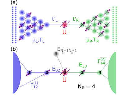
(a)

Figure 1: (Color online) (a) Sketch of the quantum impurity model Eq. (1) consisting of an impurity with interaction $U$ coupled via hybridizations $t^{\prime}_{\lambda}$ to noninteracting leads at chemical potential $\mu_{\lambda}$ and temperature $T_{\lambda}$, $\lambda\in\{L,R\}$. (b) Illustration of the auxiliary open quantum system Eq. (10a) with single particle parameters $E_{\mu\nu}$ and Lindblad dissipators $\Gamma^{\kappa}_{\mu\nu}$ consisting of the impurity at site $f=0$, $N_{B}$ bath sites ($N_{B}=4$ in the plot) as well as a Markovian environment (shaded areas). When evaluating linear corrections (see Sec. C), an additional site $N_{B}+1$ is used.

We consider a single Anderson impurity coupled to electronic leads under bias voltage (see Fig. 1 (a))

$$\hat{\mathcal{H}} =\hat{\mathcal{H}}_{\text{imp}}+\hat{\mathcal{H}}_{\text{res}}+\hat{\mathcal{H}}_{\text{coup}}\,\mbox{.}$$ (1)

The impurity orbital features charge as well as spin degrees of freedom and is subject to a local Coulomb repulsion $U$

$$\hat{\mathcal{H}}_{\text{imp}} =\epsilon_{f}\,\sum\limits_{\sigma}\,f_{\sigma}^{\dagger}\,f_{\sigma}^{\phantom{{\dagger}}}+U\,\hat{n}^{f}_{\uparrow}\,\hat{n}^{f}_{\downarrow}\,\mbox{.}$$

Here $f_{\sigma}^{\dagger}/f_{\sigma}^{\phantom{{\dagger}}}$ denote fermionic creation/annihilation operators for the impurity orbital with spin $\sigma\in\{\uparrow,\downarrow\}$ respectively. The particle number operator is defined in the usual way $\hat{n}^{f}_{\sigma}=f_{\sigma}^{\dagger}f_{\sigma}^{\phantom{{\dagger}}}$ and the impurity on-site potential is $\epsilon_{f}=(V_{G}-\frac{U}{2})$, with gate voltage $V_{G}=0$ at particle hole symmetry. The impurity is coupled to two noninteracting electronic leads $\lambda\in\{L,R\}$ with dispersion $\epsilon_{\lambda k}$

$$\hat{\mathcal{H}}_{\text{res}} =\sum\limits_{\lambda k\sigma}\left(\epsilon_{\lambda}+\epsilon_{\lambda k}\right)\,c_{k\lambda\sigma}^{\dagger}\,c_{k\lambda\sigma}^{{\phantom{{\dagger}}}}\,\mbox{.}$$

The effect of a bias voltage $\phi$ is to shift the chemical potential and the on-site energies of the two leads by $\epsilon_{\lambda}=\pm\frac{\phi}{2}$, respectively. For the energies $\epsilon_{\lambda k}$ of the leads we will consider two cases: (i) Two tight-binding semi-infinite chains with nearest-neighbor hopping $t$, corresponding to a semi-circular electronic density of states (DOS). In this case, the boundary retarded single particle Green’s function of the two uncoupled leads is given by foo (a, b); Economou (2006)

$$g_{\lambda}^{R}(\omega) =g_{\text{SC},\lambda}^{R}(\omega)=\frac{\omega-\epsilon_{\lambda}}{2t^{2}}-i\frac{\sqrt{4t^{2}-(\omega-\epsilon_{\lambda})^{2}}}{2t^{2}}\,\mbox{,}$$ (2)

with a bandwidth of $D_{SC}^{\phantom{{\dagger}}}=4\,t$. (ii) A constant DOS with a bandwidth $D_{\text{WB}}^{\phantom{{\dagger}}}=\pi\,t$, resulting in boundary Green’s functions foo (b)

$$g_{\lambda}^{R}(\omega) =g_{\text{WB},\lambda}^{R}(\omega)=-\frac{1}{D_{WB}^{\phantom{{\dagger}}}}\text{ln}\left(\frac{\omega-\epsilon_{\lambda}-\frac{D_{\text{WB}}^{\phantom{{\dagger}}}}{2}}{\omega-\epsilon_{\lambda}+\frac{D_{\text{WB}}^{\phantom{{\dagger}}}}{2}}\right)\,\mbox{.}$$ (3)

The choice $D_{\text{WB}}^{\phantom{{\dagger}}}=\pi\,t$ makes sure that the DOS at $\omega=0$ of both lead types coincide. The leads are coupled to the impurity orbital by

$$\hat{\mathcal{H}}_{\text{coup}} =\sum\limits_{\lambda\sigma}t_{\lambda}^{\prime}\frac{1}{\sqrt{N_{k}}}\sum_{k}\left(c_{k\lambda\sigma}^{\dagger}\,f_{\sigma}^{\phantom{{\dagger}}}+f_{\sigma}^{\dagger}\,c_{k\lambda\sigma}^{{\phantom{{\dagger}}}}\right)\,\mbox{,}$$

where we take the same hybridization $t^{\prime}_{\lambda}=-0.3162\,t$ for both leads, and $N_{k}\to\infty$ is the number of $k$ points. Expressions presented below are valid for arbitrary temperatures, although we will show results for zero temperature only, which is numerically the most unfavorable case. foo (c) The setup chosen here represents by no means a limitation of the method and extensions to more complicated situations, such as non-symmetric couplings, off particle-hole symmetry, etc. are straightforward.

II.2 Steady state non-equilibrium Green’s functions

We are interested in the steady state behavior under bias voltage of the model described by Eq. (1). We assume that such a steady state exists and is unique. foo (d) We denote the single particle Green’s function of the impurity in the non-equilibrium Green’s function (Keldysh) formalism by Kadanoff and Baym (1962); Schwinger (1961); Keldysh (1965); Haug and Jauho (1998); Rammer and Smith (1986)

$$\underline{G}(\omega) =\begin{pmatrix}G^{R}(\omega)&G^{K}(\omega)\\ 0&G^{A}(\omega)\end{pmatrix}\,\mbox{.}$$ (4)

Fourier transformation to energy $\omega$ is possible since in the steady state the system becomes time translationally invariant. In that case, the memory of the initial condition has been fully washed away, so there is no contribution from the Matsubara branch. Kamenev (2011) We will use an underline $\underline{\cdots}$ to denote two-point functions with the Keldysh matrix structure as in Eq. (4).

The Green’s function of the correlated impurity can be expressed via Dyson’s equation

$$\underline{G}^{-1}(\omega) =\underline{G}^{-1}_{0}(\omega)-\underline{\Sigma}(\omega)\,\mbox{,}$$ (5)

where $\underline{\Sigma}(\omega)$ is the impurity self-energy. The noninteracting impurity Green’s function $\underline{G}_{0}(\omega)$ can be written in the form

$$\underline{G}^{-1}_{0}(\omega) =\underline{g}^{-1}_{0}(\omega)-\underline{\Delta}(\omega)\,\mbox{,}$$ (6)

$\underline{g}_{0}^{\phantom{{\dagger}}}(\omega)$ being the noninteracting Green’s function of the disconnected impurity, foo (a) and

$$\underline{\Delta}(\omega) =\sum\limits_{\lambda}t_{\lambda}^{\prime\ 2}\,\underline{g}_{\lambda}^{\phantom{{\dagger}}}(\omega)\,\mbox{,}$$ (7)

is the hybridization function of the leads (a $2\times 2$ Keldysh object, in contrast to the equilibrium case, where it is convenient to work in Matsubara space). We define an equilibrium Anderson width Cyril (1997) for each lead $\Delta_{0}\equiv-\frac{1}{2}\Im{m}\,(\underline{\Delta}^{R}(\omega=0))=\frac{t^{\prime 2}_{\lambda}}{t}\approx 0.1\,t$. Below, we will use $\Delta_{0}$ as a unit of energy and in addition we choose $\hbar=e=1$.

The boundary Green’s functions $\underline{g}_{\lambda}$ of each disconnected lead is determined by (a) its retarded component $g_{\lambda}^{R}$ (either (2) or (3)), (b) its advanced component $g_{\lambda}^{A}=g_{\lambda}^{R*}$, and (c) its Keldysh component, which satisfies the fluctuation dissipation theorem

$$g_{\lambda}^{K}(\omega) =2i\left(1-2p_{\text{F}}(\omega-\mu_{\lambda})\right)\Im{m}\,(g_{\lambda}^{R}(\omega))\,\mbox{,}$$ (8)

since the disconnected leads are in equilibrium. Here, $p_{\text{F}}(\omega-\mu_{\lambda})$ is the Fermi distribution with chemical potential $\mu_{\lambda}$. For the noninteracting isolated impurity one can take $\left(g_{0}^{-1}\right)^{R}=\omega-\epsilon_{f}$, and $\left(g_{0}^{-1}\right)^{K}=0$, since infinitesimals $0^{+}$ can be neglected after coupling to the leads (unless there are bound states).

As usual, the presence of the interaction $U$ makes the solution of the problem impurity plus leads a major challenge both in equilibrium as well as out of equilibrium, which we plan to address in the present paper.

Similarly to the equilibrium case, the action of the leads on the impurity is completely determined by the hybridization function $\underline{\Delta}(\omega)$, independently of how the leads are represented in detail. In other words, if one constructs a different configuration of leads (e.g. with more leads with different temperatures, DOS, etc.), which has the same $\underline{\Delta}(\omega)$, i.e. the same $\Delta^{R}(\omega)$ and $\Delta^{K}(\omega)$ as Eq. (7), then the resulting local properties of the interacting impurity, e.g. the Green’s function $\underline{G}(\omega)$ are the same. This holds provided the leads contain noninteracting fermions only.

The approach we suggested in Ref. Arrigoni et al., 2013 precisely exploits this property. The idea is to replace the impurity plus leads system (Eq. (1)) by an auxiliary one which reproduces $\underline{\Delta}(\omega)$ as accurately as possible, and at the same time can be solved exactly by numerical methods, such as Lanczos exact diagonalization. Details on the construction of the auxiliary impurity system are given below.

The self energy $\underline{\Sigma}_{\text{aux}}(\omega)$ of the auxiliary system, obtained by exact diagonalization, is used in analogy to DMFT Caffarel and Krauth (1994); Georges et al. (1996) as an approximation to the physical self energy of the original impurity system. Inserting $\underline{\Sigma}(\omega)\approx\underline{\Sigma}_{\text{aux}}(\omega)$ into Eqs. (5), (6), together with the exact hybridization function $\underline{\Delta}(\omega)$ yields an approximation for the physical Green’s function. From this, observables such as the current or the spectral function are then calculated. We emphasize that the accuracy of this approximation can be controlled by the difference between the $\underline{\Delta}_{\text{aux}}(\omega)$ of the auxiliary system and the physical one $\underline{\Delta}(\omega)$, and that this can be, in principle, systematically improved, as discussed below.

II.3 Auxiliary open quantum system

The idea presented here is strongly related to the ED approach for the DMFT impurity problem in equilibrium. Caffarel and Krauth (1994); Georges et al. (1996) Here, the infinite leads are replaced by a small number of bath sites, whose parameters are optimized by fitting the hybridization function in Matsubara space. The reduced system of bath sites plus impurity is then solved by Lanczos ED. Lanczos (1951) This approach cannot be straightforwardly extended to the non-equilibrium steady state case for several reasons: (i) since the small bath is finite, its time dependence is (quasi) periodic, i.e. no steady state is reached, (ii) there is no Matsubara representation out of equilibrium, foo (e) thus, one is forced to use real energies but (iii) in this case $\Im{m}\,(\Delta^{R}_{\text{aux}}(\omega))$ of the small bath consists of $\delta$-peaks and can hardly be fitted to a smooth $\Delta^{R}(\omega)$. The solution we suggested in Ref. Arrigoni et al., 2013 consists in additionally coupling the small bath to a Markovian environment, which makes it effectively “infinitely large”, and solves problems (i) and (iii) above. Specifically, we replace the impurity plus leads model (Eq. (1)) by an auxiliary open quantum system consisting of the impurity plus a small number of bath sites, which in turn are coupled to a Markovian environment.

The dynamics of the system (consisting of bath sites and impurity), including the effect of the Markovian environment is expressed in terms of the Lindblad quantum master equation which controls the time dependence of its reduced density operator $\hat{\rho}$: Breuer and Petruccione (2009); Carmichael (2002)

$$\dot{\hat{\rho}} =\hat{\hat{\mathcal{L}}}\hat{\rho}\,\mbox{.}$$ (9)

The Lindblad super-operator foo (f)

$$\hat{\hat{\mathcal{L}}} =\hat{\hat{\mathcal{L}}}_{H}+\hat{\hat{\mathcal{L}}}_{D}\,\mbox{,}$$ (10a)

consists of a unitary contribution

$$\hat{\hat{\mathcal{L}}}_{H}\hat{\rho} =-i[\hat{\mathcal{H}}_{\text{aux}},\hat{\rho}]\,\mbox{,}$$

as well as a non-unitary, dissipative term originating from the coupling to the Markovian environment

$$\hat{\hat{\mathcal{L}}}_{D}\hat{\rho} \equiv 2\sum\limits_{\mu\nu=0}^{N_{B}}\sum\limits_{\sigma}\Bigg{(}\Gamma_{\nu\mu}^{(1)}\left(d_{\mu\sigma}^{\phantom{{\dagger}}}\hat{\rho}\ d_{\nu\sigma}^{{\dagger}}-\frac{1}{2}\{\hat{\rho},d_{\nu\sigma}^{{\dagger}}d_{\mu\sigma}^{\phantom{{\dagger}}}\}\right)+$$

$$+\Gamma_{\nu\mu}^{(2)}\left(d_{\nu\sigma}^{{\dagger}}\hat{\rho}\ d_{\mu\sigma}^{\phantom{{\dagger}}}-\frac{1}{2}\{\hat{\rho},d_{\mu\sigma}^{\phantom{{\dagger}}}d_{\nu\sigma}^{{\dagger}}\}\right)\Bigg{)}\,\mbox{,}$$ (10b)

where $[\hat{A},\hat{B}]$ and $\{\hat{A},\hat{B}\}$ denote the commutator and anti-commutator respectively. The unitary time evolution is generated by the Hamiltonian

$$\hat{\mathcal{H}}_{\text{aux}} =\sum\limits_{\mu\nu=0}^{N_{B}}\sum\limits_{\sigma}E_{\mu\nu}d_{\mu\sigma}^{{\dagger}}d_{\nu\sigma}^{\phantom{{\dagger}}}+Ud_{f\uparrow}^{{\dagger}}d_{f\uparrow}^{\phantom{{\dagger}}}d_{f\downarrow}^{{\dagger}}d_{f\downarrow}^{\phantom{{\dagger}}}\,\mbox{,}$$ (11)

describing a fermionic “chain” ($E_{\mu\nu}$ is non-zero only for on-site and nearest neighbor terms). It is convenient to choose the interacting impurity at site $f=0$ and $N_{B}$ auxiliary bath sites at $\mu,\nu=1,\cdots,N_{B}$ (see Fig. 1). As usual, $d_{\mu\sigma}^{\dagger}/d_{\mu\sigma}^{\phantom{{\dagger}}}$ create/annihilate the corresponding auxiliary particles. The quadratic form of the dissipator (Eq. (10b)) corresponds to a noninteracting Markovian environment. The dissipation matrices $\Gamma_{\mu\nu}^{(\kappa)}$, $\kappa\in\{1,2\}$ are hermitian and positive semidefinite. Breuer and Petruccione (2009) The advantage of replacing the impurity problem by the auxiliary one described by Eqs. (9)-(11), is that for a small number of bath sites the dynamics of the interacting auxiliary system can be solved exactly by diagonalization of the super-operator $\hat{\hat{\mathcal{L}}}$ in the space of many-body density operators (see Sec. II.4.2).

Intuitively, one can consider the effective system as a truncation of the original chain described by Eq. (1), whereby the Markovian environment compensates for the missing “pieces”. However, this would still be a crude approximation, and in addition, it would not be clear how to introduce the chemical potential in the Markovian environment (except for weak coupling). Our strategy, similarly to the equilibrium case, consists in simply using the parameters of the auxiliary system in order to provide an optimal fit to the bath spectral function $\underline{\Delta}(\omega)$. The parameters for the fit are, in principle, $E_{\mu\nu}$ and $\Gamma_{\mu\nu}^{(\kappa)}$. However, one should consider that there is a certain redundancy. In other words several combinations of parameters lead to the same $\underline{\Delta}(\omega)$. For example, it is well known in equilibrium that in the case of the $E_{\mu\nu}$ one can restrict to diagonal and nearest neighbor terms only. foo (g)

The accuracy of the results will be directly related to the accuracy of the fit to $\underline{\Delta}(\omega)$, and this is expected to increase rapidly with the number of fit parameters, which obviously increases with $N_{B}$. On the other hand, also the computational complexity necessary to exactly diagonalize the interacting auxiliary system increases exponentially with $N_{B}$. The fit does not present a major numerical difficulty, as the determination of the hybridization functions of both the original model (Eq. (7)), as well as the one of the auxiliary system $\underline{\Delta}_{\text{aux}}(\omega)$ described by the Lindblad equation (10) require the evaluation of $\underline{G}_{0}$ (cf. (6)), i.e. the solution of a noninteracting problem.

The fit is obtained by minimizing the cost function

$$\chi(E_{\mu\nu},\Gamma_{\mu\nu}^{(\kappa)})= \sum\limits_{\alpha\in\{R,K\}}\int\limits_{-\infty}^{\infty}d\omega\,W^{\alpha}(\omega)$$

$$\times\left|\Delta^{\alpha}(\omega)-\Delta^{\alpha}_{\text{aux}}(\omega;E_{\mu\nu},\Gamma_{\mu\nu}^{(\kappa)})\right|^{n}\,\mbox{.}$$ (12)

with respect to the parameters of the auxiliary system. The advanced component does not need to be considered as $\Delta^{A}=\Delta^{R*}$. Of course, like in ED based DMFT, there exists an ambiguity which is related to the choice of the weight function $W^{\alpha}(\omega)$, which also sets the integral boundaries. This uncertainty is clearly reduced upon increasing $N_{B}$.

Depending on the expected physics, it might be useful to adopt a energy-dependent weight function. This could be used for example to describe the physics around the chemical potentials more accurately.

Once the auxiliary system is defined in terms of $E_{\mu\nu}\mbox{ and }\Gamma_{\mu\nu}^{(\kappa)}$, the corresponding interacting non-equilibrium problem Eq. (10) can be solved by an exact diagonalization of the non-hermitian super-operator $\hat{\hat{\mathcal{L}}}$ within the space of many-body density operators. The dimension of this space is equal to the square of the dimension of the many-body Hilbert space, and thus it grows exponentially as a function of $N_{B}$. Therefore, for $N_{B}\geq 4$ a non-hermitian Lanczos treatment must be used. The solution of the noninteracting Lindblad problem is non standard (see e.g. Ref. Prosen, 2008), and a method particularly suited for the present approach is discussed in Sec. II.4.1.

II.4 Green’s functions of the auxiliary Lindblad problem

In this section we present expressions for the Green’s functions of the auxiliary system. Specifically, we will derive an analytic expression for the noninteracting Green’s functions in Sec. II.4.1, and illustrate the numerical procedure to determine the interacting ones in Sec. II.4.2. The derivations make largely use of the formalism of Ref. Dzhioev and Kosov, 2011, see also Ref. Schmutz, 1978. For an alternative appealing approach to the noninteracting case, see also Ref. Prosen, 2008. All Green’s functions discussed in Sec. II.4 are the ones of the auxiliary system, which are different from the physical ones for $N_{B}<\infty$.

The dynamics of the auxiliary open quantum system described by the super-operator $\hat{\hat{\mathcal{L}}}$ (Eq. (10)) can be recast in an elegant way as a standard operator problem in an augmented fermion Fock space with twice as many sites. Dzhioev and Kosov (2011); Schmutz (1978); Harbola and Mukamel (2008); Prosen (2008) Specifically, one introduces “tilde” operators $\tilde{d}_{\mu}^{\phantom{{\dagger}}}/\tilde{d}_{\mu}^{\dagger}$ together with the original ones ${d}_{\mu}^{\phantom{{\dagger}}}/{d}_{\mu}^{\dagger}$. foo (h) Introducing the so-called left-vacuum

$$\mathinner{|{I}\rangle} =\sum\limits_{S}(-i)^{N_{S}}\mathinner{|{S}\rangle}\otimes\mathinner{|{\tilde{S}}\rangle}\,\mbox{,}$$ (13)

where $\mathinner{|{S}\rangle}$ are many-body states of the original Fock space, $\mathinner{|{\tilde{S}}\rangle}$ the corresponding ones of the tilde space Dzhioev and Kosov (2011) and $N_{S}$ the number of particles in $S$. The non-equilibrium density operator can be written as a state vector in this augmented space

$$\mathinner{|{\rho(t)}\rangle}\equiv\hat{\rho}(t)\mathinner{|{I}\rangle}\,.$$ (14)

The Lindblad equation is rewritten in a Schrödinger like fashion Dzhioev and Kosov (2011); foo (f)

$$\frac{d}{dt}\mathinner{|{\rho(t)}\rangle} =\hat{\mathcal{L}}\mathinner{|{\rho(t)}\rangle}\,\mbox{,}$$ (15)

where now $\hat{\mathcal{L}}$ is an ordinary operator in the augmented space. $\hat{\mathcal{L}}=\hat{\mathcal{L}}_{0}+\hat{\mathcal{L}}_{I}$ is conveniently represented in terms of the operators of the augmented space in a vector notation: foo (h)

$$\boldsymbol{d}^{\dagger} =\left(d_{0}^{\dagger},\ldots,d_{N_{B}}^{\dagger},\tilde{d}_{0},\ldots\tilde{d}_{N_{B}}\right)\,\mbox{.}$$

Its noninteracting part $\mathcal{L}_{0}$ reads in the augmented space Dzhioev and Kosov (2011); foo (f)

$$i\hat{\mathcal{L}}_{0} =\sum\limits_{\sigma}\left(\boldsymbol{d}^{\dagger}\boldsymbol{h}\boldsymbol{d}-\,\text{Tr}\left(\boldsymbol{E}+i\boldsymbol{\Lambda}\right)\right)\,\mbox{,}$$ (16)

where Tr denotes the matrix trace and the matrix $\boldsymbol{h}$ is given by

$$\boldsymbol{h} =\begin{pmatrix}\boldsymbol{E}+i\boldsymbol{\Omega}&2\boldsymbol{\Gamma}^{(2)}\\ -2\boldsymbol{\Gamma}^{(1)}&\boldsymbol{E}-i\boldsymbol{\Omega}\end{pmatrix}\,\mbox{,}$$ (17)

with

$$\boldsymbol{\Lambda}=\left(\boldsymbol{\Gamma}^{(2)}+\boldsymbol{\Gamma}^{(1)}\right)\,\mbox{,} \quad\quad\boldsymbol{\Omega}=\left(\boldsymbol{\Gamma}^{(2)}-\boldsymbol{\Gamma}^{(1)}\right)\,\mbox{.}$$

Its interacting part has the form Dzhioev and Kosov (2011)

$$i\mathcal{L}_{I} =Ud^{\dagger}_{f\uparrow}d^{\phantom{{\dagger}}}_{f\uparrow}d^{\dagger}_{f\downarrow}d^{\phantom{{\dagger}}}_{f\downarrow}-U\tilde{d}^{\dagger}_{f\uparrow}\tilde{d}^{\phantom{{\dagger}}}_{f\uparrow}\tilde{d}^{\dagger}_{f\downarrow}\tilde{d}^{\phantom{{\dagger}}}_{f\downarrow}\,\mbox{.}$$

In this auxiliary open system, dynamic two-time correlation functions for two operators $\hat{A}$ and $\hat{B}$ of the system can be expressed as

$$iG_{BA}(t_{2},t_{1}) \equiv\langle\hat{B}{}_{\cal U}(t_{2})\hat{A}{}_{\cal U}(t_{1})\rangle=\text{tr}\,_{{\cal U}}\left(\hat{B}{}_{\cal U}(t_{2})\hat{A}{}_{\cal U}(t_{1})\hat{\rho}_{\cal U}\right)$$

$$=\text{tr}\,\left(\hat{B}\hat{A}_{t_{1},t_{2}-t_{1}}\right)\,\mbox{,}$$ (18)

where $\hat{\rho}_{\cal U}$ is the density operator of the “universe” ${\cal U}$ composed of the system and Markovian environment, tr is the trace over the system degrees of freedom, $\text{tr}\,_{E}$ the one over the environment, $\text{tr}\,_{{\cal U}}=\text{tr}\,\otimes\text{tr}\,_{E}$ the one over the universe, $\hat{O}{}_{\cal U}(\cdots)$ denotes the unitary time evolution of an operator $\hat{O}$ according to the Hamiltonian of the universe $\hat{\mathcal{H}}_{\cal U}$. Here, Carmichael (2002)

$$\hat{A}_{t_{1},t} \equiv\text{tr}\,_{E}\left(e^{-i\hat{\mathcal{H}}_{\cal U}t}\hat{A}\hat{\rho}_{{\cal U}}(t_{1})e^{+i\hat{\mathcal{H}}_{\cal U}t}\right)\,\mbox{.}$$ (19)

Notice that the time evolution of $\hat{\rho}_{\cal U}(t)$, as well as the one in Eq. (19) are opposite with respect to the Heisenberg time evolution of operators. This is the convention for density operators. For $t=t_{2}-t_{1}>0$ one can use the quantum regression theorem Carmichael (2002) which holds under the same assumptions as for Eq. (9). It states that

$$\frac{d}{dt}\hat{A}_{t_{1},t} =\hat{\hat{\mathcal{L}}}\hat{A}_{t_{1},t}\,\mbox{.}$$ (20)

In the augmented space, in the same way as for (14)-(15), one can associate the operator (19) with the state vector $\mathinner{|{A_{t_{1},t}}\rangle}=\hat{A}_{t_{1},t}\mathinner{|{I}\rangle}$. For this vector, (20) translates into

$$\frac{d}{dt}\mathinner{|{A_{t_{1},t}}\rangle} =\hat{\mathcal{L}}\mathinner{|{A_{t_{1},t}}\rangle}\,\mbox{.}$$ (21)

Considering its initial value (time $t=0$)

$$\mathinner{|{A_{t_{1},0}}\rangle} =\hat{A}\mathinner{|{\rho(t_{1})}\rangle}\,\mbox{,}$$

the solution of (21) reads

$$\mathinner{|{A_{t_{1},t}}\rangle} =e^{\hat{\mathcal{L}}t}\hat{A}\mathinner{|{\rho(t_{1})}\rangle}\,\mbox{.}$$ (22)

Therefore, we have for the correlation function (II.4) for $t_{2}>t_{1}$, which we denote as $G_{BA}^{+}(t_{2},t_{1})$

$$iG_{BA}^{+}(t_{2},t_{1}) =\mathinner{\langle{I}|}\hat{B}e^{\hat{\mathcal{L}}(t_{2}-t_{1})}\hat{A}\mathinner{|{\rho(t_{1})}\rangle}$$

$$=\mathinner{\langle{I}|}\hat{B}(t_{2}-t_{1})\hat{A}\mathinner{|{\rho(t_{1})}\rangle}\,\mbox{,}$$

where

$$\hat{B}(t) :=e^{-\hat{\mathcal{L}}t}\hat{B}e^{\hat{\mathcal{L}}t}\,\mbox{,}$$ (23)

is the non-hermitian time evolution of the operator $\hat{B}$, and we have exploited the relation Dzhioev and Kosov (2011) $\mathinner{\langle{I}|}\hat{\mathcal{L}}=0$. For the steady state correlation function, which depends on $t=t_{2}-t_{1}$, we have

$$iG_{BA}^{+}(t) =\mathinner{\langle{I}|}\hat{B}(t)\hat{A}\mathinner{|{\rho_{\infty}}\rangle}\,\mbox{,}$$ (24)

where $\hat{\rho}_{\infty}$ is the steady state density operator. Since the quantum regression theorem only propagates forward in time, for $t<0$ one has to take the complex conjugate of Eq. (II.4), which gives for the $t<0$ steady state correlation function denoted as $G_{BA}^{-}$:

$$iG_{BA}^{-}(t) =-iG_{A^{\dagger}B^{\dagger}}^{+}(-t)^{*}=\mathinner{\langle{I}|}\hat{A}^{\dagger}(-t)\hat{B}^{\dagger}\mathinner{|{\rho_{\infty}}\rangle}^{*}\,\mbox{.}$$ (25)

Using (24), the steady state greater Green’s function for times $t>0$ reads foo (i)

$$G_{\mu\nu}^{>+}(t) \equiv-i\theta(t)\ \left<d_{\mu}^{\phantom{{\dagger}}}(t+t_{1})d^{\dagger}_{\nu}(t_{1})\right>_{t1\to\infty}$$

$$=-i\theta(t)\ \mathinner{\langle{I}|}d_{\mu}^{\phantom{{\dagger}}}(t)d^{\dagger}_{\nu}\mathinner{|{\rho_{\infty}}\rangle}\,\mbox{.}$$ (26)

We can use (24) also for the lesser Green’s function, however for foo (i) $t<0$

$$G_{\mu\nu}^{<+}(t) \equiv i\theta(-t)\ \left<d_{\nu}^{\dagger}(t_{1})d^{\phantom{{\dagger}}}_{\mu}(t+t_{1})\right>_{t1\to\infty}$$

$$=i\theta(-t)\ \mathinner{\langle{I}|}d_{\nu}^{\dagger}(-t)d^{\phantom{{\dagger}}}_{\mu}\mathinner{|{\rho_{\infty}}\rangle}\,\mbox{.}$$

For the opposite sign of $t$, we can use (25), so that for both Green’s functions one has foo (f, i)

$$\boldsymbol{G}^{\stackrel{{\scriptstyle>}}{{<}}-}(t) =-\boldsymbol{G}^{\stackrel{{\scriptstyle>}}{{<}}+}(-t)^{\dagger}\,\mbox{.}$$ (27)

For the Fourier transformed Green’s function, defined, with abuse of notation as

$$\boldsymbol{G}^{\stackrel{{\scriptstyle>}}{{<}}\pm}(\omega) =\int dt\ e^{i\omega t}\boldsymbol{G}^{\stackrel{{\scriptstyle>}}{{<}}\pm}(t)\,\mbox{,}$$ (28)

relation (27) translates into

$$\boldsymbol{G}^{\stackrel{{\scriptstyle>}}{{<}}-}(\omega) =-\boldsymbol{G}^{\stackrel{{\scriptstyle>}}{{<}}+}(\omega)^{\dagger}\,\mbox{.}$$ (29)

We need the retarded and the Keldysh Green’s functions

$$\boldsymbol{G}^{R}=\boldsymbol{G}^{>+}-\boldsymbol{G}^{<-}=\boldsymbol{G}^{>+}+\boldsymbol{G}^{<+{\dagger}}\,\mbox{,}$$ (30)

$$\boldsymbol{G}^{K}=\boldsymbol{G}^{>+}+\boldsymbol{G}^{<-}+\boldsymbol{G}^{>-}+\boldsymbol{G}^{<+}=\boldsymbol{G}^{>+}+\boldsymbol{G}^{<+}-h.c.\,\mbox{,}$$

whereby both relations hold for the time-dependent as well as for the Fourier transformed ones.

II.4.1 Noninteracting case

To solve the noninteracting Lindblad problem described by (16), one first diagonalizes the non-hermitian matrix Dzhioev and Kosov (2011) $\boldsymbol{h}$ in (17):

$$\boldsymbol{\varepsilon} ={\boldsymbol{V}}^{-1}\boldsymbol{h}{\boldsymbol{V}}\,\mbox{,}$$ (31)

where $\boldsymbol{\varepsilon}$ is a diagonal matrix of eigenvalues $\varepsilon_{\mu}$. The noninteracting Lindbladian Eq. (16) can then be written as

$$i\hat{\mathcal{L}}_{0} =\boldsymbol{\bar{\xi}}\ \boldsymbol{\varepsilon}\ \boldsymbol{\xi}+\eta\,\mbox{,}$$

in terms of the normal modes

$$\boldsymbol{\xi} ={\boldsymbol{V}}^{-1}\boldsymbol{d}\,\mbox{,}\quad\quad\boldsymbol{\bar{\xi}}=\boldsymbol{d}^{\dagger}{\boldsymbol{V}}\,\mbox{,}$$ (32)

and a constant $\eta$. The normal modes still obey canonical anticommutation rules

$$\{\xi_{\mu},\bar{\xi}_{\nu}\} =\delta_{\mu\nu}\,\mbox{,}$$ (33)

but are not mutually hermitian conjugate.

The steady state $\mathinner{|{\rho_{\infty}}\rangle}$ obeys the equation

$$\hat{\mathcal{L}}\mathinner{|{\rho_{\infty}}\rangle} =0\,\mbox{.}$$

Let us now consider the time evolution (22) of a state initially consisting of the normal mode operators applied to the steady state density matrix:

$$e^{\hat{\mathcal{L}}_{0}t}\xi_{\mu}\mathinner{|{\rho_{\infty}}\rangle} =e^{\hat{\mathcal{L}}_{0}t}\xi_{\mu}e^{-\hat{\mathcal{L}}_{0}t}\mathinner{|{\rho_{\infty}}\rangle}=e^{i\varepsilon_{\mu}t}\xi_{\mu}\mathinner{|{\rho_{\infty}}\rangle}\,\mbox{.}$$

If $\Im{m}\,(\varepsilon_{\mu})<0$ this term diverges exponentially in the long-time limit, which would be in contradiction to the fact that $\mathinner{|{\rho_{\infty}}\rangle}$ is a steady state, unless the state created by $\xi_{\mu}$ is zero. Therefore, we must have

$$\xi_{\mu}\mathinner{|{\rho_{\infty}}\rangle} =0\quad\quad\hbox{ for }\Im{m}\,(\varepsilon_{\mu})<0\,\mbox{.}$$ (34a)

Similarly, we must have

$$\bar{\xi}_{\mu}\mathinner{|{\rho_{\infty}}\rangle} =0\quad\quad\hbox{ for }\Im{m}\,(\varepsilon_{\mu})>0\,\mbox{.}$$ (34b)

These equations, thus, define the steady state as a kind of “Fermi sea”. In addition, by requiring that expectation values of the form

$$\mathinner{\langle{I}|}\xi_{\mu}(t)\bar{\xi}_{\nu}\mathinner{|{\rho}\rangle}\,\mbox{,}$$

do not diverge for large $$t$$, we obtain that

$$\mathinner{\langle{I}|}\xi_{\mu} =0\quad\quad\hbox{ for }\Im{m}\,(\varepsilon_{\mu})>0\,\mbox{,}$$ (34c)

$$\mathinner{\langle{I}|}\bar{\xi}_{\mu} =0\quad\quad\hbox{ for }\Im{m}\,(\varepsilon_{\mu})<0\,\mbox{.}$$ (34d)

From (34d) it follows that an expectation value of the form $\mathinner{\langle{I}|}\bar{\xi}_{\mu}\xi_{\nu}\mathinner{|{\rho_{\infty}}\rangle}$ vanishes for the case $\Im{m}\,(\varepsilon_{\mu})<0$. For $\Im{m}\,(\varepsilon_{\mu})>0$ we make use of the anticommutation rules (33) together with (34b) and the fact that Dzhioev and Kosov (2011) $\mathinner{\langle{I|\rho_{\infty}}\rangle}=\text{tr}\,\rho_{\infty}=1$ and arrive at

$$\mathinner{\langle{I}|}\bar{\xi}_{\mu}\xi_{\nu}\mathinner{|{\rho_{\infty}}\rangle} =D_{\mu\nu}\,\mbox{,}$$

where the matrix

$$D_{\mu\nu} =\delta_{\mu\nu}\ \theta({\Im{m}\,(\varepsilon_{\mu}}))\,\mbox{.}$$

Similarly,

$$\mathinner{\langle{I}|}\xi_{\mu}\bar{\xi}_{\nu}\mathinner{|{\rho_{\infty}}\rangle} =\bar{D}_{\mu\nu}\equiv\delta_{\mu\nu}-D_{\mu\nu}\,\mbox{.}$$

The expression for the steady state correlation functions of the eigenmodes $\boldsymbol{\xi}$ of $\hat{\mathcal{L}}_{0}$ can be now evaluated by considering that, due to the anticommutation rules the Heisenberg time evolution (23) gives

$$\xi_{\mu}(t) =e^{-i\varepsilon_{\mu}t}\ \xi_{\mu}\,\mbox{,}\quad\quad\bar{\xi}_{\mu}(t)=e^{i\varepsilon_{\mu}t}\ \bar{\xi}_{\mu}\,\mbox{.}$$

Thus,

$$\mathinner{\langle{I}|}\xi_{\mu}^{\phantom{{\dagger}}}(t)\bar{\xi}^{\phantom{{\dagger}}}_{\nu}\mathinner{|{\rho_{\infty}}\rangle} =e^{-i\varepsilon_{\mu}t}\mathinner{\langle{I}|}\xi_{\mu}^{\phantom{{\dagger}}}\bar{\xi}^{\phantom{{\dagger}}}_{\nu}\mathinner{|{\rho_{\infty}}\rangle}=e^{-i\varepsilon_{\mu}t}D_{\mu\nu}\,\mbox{.}$$

In this way, the greater Green’s function for $t>0$ becomes

$$iG_{0\mu\nu}^{>+}(t)=\mathinner{\langle{I}|}d_{\mu}^{\phantom{{\dagger}}}(t)d^{\dagger}_{\nu}\mathinner{|{\rho_{\infty}}\rangle}$$ (35)

$$=\sum\limits_{\varsigma}V_{\mu\varsigma}e^{-i\varepsilon_{\varsigma}t}\bar{D}_{\varsigma\varsigma}(V^{-1})_{\varsigma\nu}=\left({\boldsymbol{V}}e^{-i\boldsymbol{\varepsilon}t}\boldsymbol{\bar{D}}{\boldsymbol{V}}^{-1}\right)_{\mu\nu}\,\mbox{,}$$

where we have used (32). The Green’s functions are defined with operators $d_{\mu}^{\phantom{{\dagger}}}/d^{\dagger}_{\mu}$ in the original Fock space, so that it is sufficient to know the first $N_{B}+1$ rows (columns) of ${\boldsymbol{V}}$ (${\boldsymbol{V}}^{-1}$). For this purpose we introduce

$$\boldsymbol{U} =\boldsymbol{T}{\boldsymbol{V}}\,,$$

$$\boldsymbol{U}^{(-1)} ={\boldsymbol{V}}^{-1}\boldsymbol{T}^{\dagger}\,\mbox{,}$$

whereby $\boldsymbol{T}$ is a $(N_{B}+1)\times(2N_{B}+2)$ matrix, which in block form reads $\boldsymbol{T}=(11\hskip 10.00002pt\boldsymbol{0})$. Notice that $\boldsymbol{U}^{-1}\neq\boldsymbol{U}^{(-1)}$. With this, the Fourier transform (28) of (35) is given by foo (j)

$$\boldsymbol{G}^{>+}_{0}(\omega)=\left(\boldsymbol{U}\frac{\boldsymbol{\bar{D}}}{\omega-\boldsymbol{\varepsilon}}\boldsymbol{U}^{(-1)}\right)\,\mbox{,}$$ (36)

and $G_{0\mu\nu}^{>-}(\omega)$ is obtained with the help of (29). Similarly, the lesser Green’s function for $t<0$

$$iG_{0\mu\nu}^{<+}(t)=-\mathinner{\langle{I}|}d_{\nu}^{\dagger}d_{\mu}(t)\mathinner{|{\rho_{\infty}}\rangle}$$

$$=-\sum\limits_{\varsigma}V_{\mu\varsigma}e^{-i\varepsilon_{\varsigma}t}D_{\varsigma\varsigma}(V^{-1})_{\varsigma\nu}=-\left(\boldsymbol{U}e^{-i\boldsymbol{\varepsilon}t}\boldsymbol{D}\boldsymbol{U}^{(-1)}\right)_{\mu\nu}\,\mbox{,}$$

with the Fourier transform

$$\boldsymbol{G}^{<+}_{0}(\omega) =\left(\boldsymbol{U}\frac{\boldsymbol{D}}{\omega-\boldsymbol{\varepsilon}}\boldsymbol{U}^{(-1)}\right)\,\mbox{,}$$ (37)

and $\boldsymbol{G}^{<-}_{0}(\omega)$ is obtained from (29). Using (30) together with (36) and (37), we get

$$\boldsymbol{G}^{R}_{0}(\omega) =\boldsymbol{U}\frac{\boldsymbol{\bar{D}}}{\omega-\boldsymbol{\varepsilon}}\boldsymbol{U}^{(-1)}+\left(\boldsymbol{U}\frac{\boldsymbol{D}}{\omega-\boldsymbol{\varepsilon}}\boldsymbol{U}^{(-1)}\right)^{\dagger}\,\mbox{,}$$ (38)

and for the Keldysh Green’s function using also (29)

$$\boldsymbol{G}^{K}_{0}(\omega) =\boldsymbol{U}\left(\frac{\boldsymbol{\bar{D}}}{\omega-\boldsymbol{\varepsilon}}+\frac{\boldsymbol{D}}{\omega-\boldsymbol{\varepsilon}}\right)\boldsymbol{U}^{(-1)}-\hbox{h.c.}$$

$$=\boldsymbol{U}\left(\frac{1}{\omega-\boldsymbol{\varepsilon}}\right)\boldsymbol{U}^{(-1)}-\hbox{h.c.}\,\mbox{.}$$ (39)

In principle, one could just carry out the diagonalization (31) and then evaluate (38) and (II.4.1) numerically, which is a rather lightweight task. However, it is possible to obtain a (partially) analytical expression for the Green’s functions. Indeed, a lengthy but straightforward calculation yields for the retarded one

$$\boldsymbol{G}^{R}_{0}(\omega) =\left(\omega-\boldsymbol{E}+i\boldsymbol{\Lambda}\right)^{-1}\,\mbox{.}$$ (40)

Similarly, for the Keldysh component of the inverse Green’s function we obtain

$$\left(\boldsymbol{\underline{G}^{-1}_{0}}\right)^{K} \equiv-\boldsymbol{G}^{R-1}_{0}\boldsymbol{G}^{K}_{0}\boldsymbol{G}^{A-1}_{0}=-2i\boldsymbol{\Omega}\,\mbox{.}$$ (41)

To sum up, (40) and (41) are the main results of this subsection. To evaluate $\underline{\Delta}_{\text{aux}}(\omega)$, one then uses (6), whereby one should consider that the matrix $\underline{G}_{0}$ in Keldysh space is just the local one, i.e., in terms of the components local at the impurity $G^{R}_{0ff}$ and $G^{K}_{0ff}$:

$$\underline{G}_{0}\equiv\left(\begin{array}[]{cc}G^{R}_{0ff}&G^{K}_{0ff}\\[4.0pt] 0&G^{A}_{0ff}\end{array}\right)\,\mbox{.}$$

In turn, $G^{K}_{0ff}$, the $ff$ component of $\boldsymbol{G}^{K}_{0}$ has to be obtained from (41) by the well-known expression Haug and Jauho (1998) $\boldsymbol{G}^{K}_{0}=-\boldsymbol{G}^{R}_{0}\left(\boldsymbol{\underline{G}^{-1}_{0}}\right)^{K}\boldsymbol{G}^{A}_{0}\,\mbox{.}$

II.4.2 Interacting case

The next step consists in solving the interacting auxiliary Lindblad problem described by (10a) in order to determine the Green’s function and the self energy at the impurity site. This is done by Lanczos exact diagonalization within the many-body augmented Fock space.

First, the steady state $\mathinner{|{\rho_{\infty}}\rangle}$ has to be determined as the right-sided eigenstate of the Lindblad operator $\hat{\mathcal{L}}$ with eigenvalue $l_{0}=0$. For convenience we introduce

$${\hat{L}} =i\hat{\mathcal{L}}\,\mbox{,}$$ (42)

which is a kind of non-hermitian Hamiltonian with complex eigenvalues $\ell$. The dimension of the Hilbert space can be reduced by exploiting symmetries similar to the equilibrium case. The conservation of the particle number per spin $\hat{N}_{\sigma}$ is replaced here by the conservation of $\hat{N}_{\sigma}-\hat{\tilde{N}}_{\sigma}$. Arrigoni et al. (2013) The steady state lies in the sector $N_{\sigma}-\tilde{N}_{\sigma}=0$.

Starting from Eq. (26), the steady state greater Green’s function of the impurity reads in a non-hermitian Lehmann representation, for $t>0$

$$G_{\mu\nu}^{>+}(t) =-i\sum_{n}e^{-i\ell_{n}^{(+1)}t}\mathinner{\langle{I}|}d_{\mu}^{\phantom{{\dagger}}}\mathinner{|{R_{n}^{(+1)}}\rangle}\mathinner{\langle{L_{n}^{(+1)}}|}d^{\dagger}_{\nu}\mathinner{|{\rho_{\infty}}\rangle}\,\mbox{,}$$

where the identity $\sum_{n}\mathinner{|{R_{n}^{(+1)}}\rangle}\mathinner{\langle{L_{n}^{(+1)}}|}$ in the sector $N_{\sigma}-\tilde{N}_{\sigma}=+1$ has been inserted, in terms of right ($\mathinner{|{R_{n}^{(+1)}}\rangle}$) and left ($\mathinner{\langle{L_{n}^{(+1)}}|}$) eigenstates of ${\hat{L}}$ with eigenvalues $\ell_{n}^{(+1)}$, and $\mathinner{|{I}\rangle}$ is the left vacuum (13). Its Fourier transform reads

$$G_{\mu\nu}^{>}(\omega) =\sum\limits_{n}\frac{1}{\omega-\ell_{n}^{(+1)}}\mathinner{\langle{I}|}d_{\mu}^{\phantom{{\dagger}}}\mathinner{|{R_{n}^{(+1)}}\rangle}\mathinner{\langle{L_{n}^{(+1)}}|}d^{\dagger}_{\nu}\mathinner{|{\rho_{\infty}}\rangle}$$

$$-\sum_{n}\frac{1}{\omega-\ell_{n}^{(+1)*}}\left(\mathinner{\langle{I}|}d_{\nu}^{\phantom{{\dagger}}}\mathinner{|{R_{n}^{(+1)}}\rangle}\mathinner{\langle{L_{n}^{(+1)}}|}d^{\dagger}_{\mu}\mathinner{|{\rho_{\infty}}\rangle}\right)^{*}\,\mbox{.}$$ (43)

The analogous expression for the lesser Green’s function $G_{\mu\nu}^{<}(\omega)$ is obtained by inserting a complete set of eigenstates in the $N_{\sigma}-\tilde{N}_{\sigma}=-1$ sector and exchanging the elementary operators accordingly. $G_{\mu\nu}^{K}(\omega)$ and $G_{\mu\nu}^{R}(\omega)$ are obtained using Eq. (30), see also (29).

For a small number of bath sites $N_{B}\leq 3$ the dimension of the augmented Fock space is still moderate, and eigenvalues and eigenvectors can be determined by full diagonalization. For $N_{B}\geq 4$ a non-hermitian Lanczos procedure has to be carried out. Especially extracting the steady state is not an easy task, since it lies in the center of the spectrum. Details of our numerical procedure are given in App. A.

Once the interacting and non-interacting Green’s functions of the auxiliary system at the impurity site $\underline{G}(\omega)$ and $\underline{G}_{0}(\omega)$, respectively, are determined, the corresponding self energy is obtained via Dyson’s equation in Keldysh space Eq. (5). The individual components are explicitly Arrigoni et al. (2013)

$$\Sigma^{R}(\omega) =1/G_{0}^{R}(\omega)-1/G^{R}(\omega)$$

$$\Sigma^{K}(\omega) =-G_{0}^{K}(\omega)/|G_{0}^{R}(\omega)|^{2}+G^{K}(\omega)/|G^{R}(\omega)|^{2}\,\mbox{.}$$

As discussed in Sec. II.2, this is used in the Dyson equation (5) for the physical Green’s function.

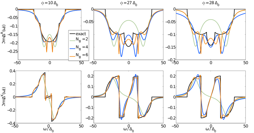
Figure 2: (Color online) Comparison of $\Im{m}\,(\Delta^{\alpha}(\omega))$ from (7) (black) with $\Im{m}\,(\Delta^{\alpha}_{\text{aux}}(\omega))$ at the absolute minimum of the cost function Eq. (12) for auxiliary system sizes $N_{B}=2,4,\mbox{ and }6$ bath sites (green, blue and orange, respectively), and $\alpha=R$ (top) and $K$ (bottom). Results are shown for tight-binding leads Eq. (2) and Eq. (8) with $t=10\,\Delta_{0}$, and three different bias voltages $\phi\in\{10,27,28\}\,\Delta_{0}$ from left to right.

III Results

In this section, results for the steady state properties of a symmetric, correlated Anderson impurity coupled to two metallic leads under bias voltage are provided. We assess the validity of the proposed method by discussing the fit of the hybridization function and outline how uncertainties are estimated. Results for the current voltage characteristics and the non equilibrium spectral function are presented and compared with data from TEBD Nuss et al. (2013) and SNRG Anders and Schmitt (2010) calculations, respectively. The effect of a linear correction of the calculated Green’s functions is illustrated.

III.1 Hybridization functions

The optimal representation of the exact bath $\underline{\Delta}(\omega)$ by the auxiliary one $\underline{\Delta}_{\text{aux}}(\omega)$ is obtained by minimizing the cost function Eq. (12). In practice this is done by employing a quasi-Newton line search. Shanno (1970); Press et al. (2007) In particular, we chose an equal weighting of the retarded and the Keldysh component $W^{R}(\omega)=W^{K}(\omega)=\Theta(\omega_{c}-|\omega|)$. After finding our results to be robust upon different values for the cut-off $\omega_{c}$, as well as upon using different norms ($n=1,2$) in Eq. (12), we finally choose $\omega_{c}=50\,\Delta_{0}$ and consider imaginary parts $\left(\Im{m}\,(\Delta^{\alpha}(\omega)-\Delta^{\alpha}_{\text{aux}}(\omega))\right)^{2}$ in the cost function only. This is justified since $\Delta_{\text{aux}}^{K}(\omega)$ is purely imaginary and the real part of $\Delta_{\text{aux}}^{R}(\omega)$ is connected to its imaginary part via the Kramers-Kronig relations. Jackson (1975) The asymptotic behavior of $\Delta^{R}_{\text{aux}}(\omega)$ is determined by $\Lambda_{ff}$ whereas the one of $\Delta^{K}_{\text{aux}}(\omega)$ by $\Omega_{ff}$. Therefore, the correct asymptotic limit $\lim\limits_{\omega\rightarrow\pm\infty}\underline{\Delta}_{\text{aux}}(\omega)=\underline{0}$ is guaranteed by taking $\Gamma^{(1)}_{ff}=\Gamma^{(2)}_{ff}=0$, which results in $\Gamma^{(\kappa)}_{\mu f}=\Gamma^{(\kappa)}_{f\mu}=0$ due to the requirement of semi-positive definiteness of $\Gamma^{(\kappa)}_{\mu\nu}$. Particle-hole symmetry allows for a further reduction of the auxiliary system parameters. foo (k)

In this work we use an even number of auxiliary bath sites $N_{B}=2,4,\mbox{ and }6$ in a linear setup (see Fig. 1 (b)) with an equal number to the left and to the right of the impurity (only Fig. 6 displays one calculation for an odd number of bath sites). In Fig. 2, the obtained auxiliary hybridization functions are compared with the exact ones for various bias voltages. We find a quick convergence as a function of $N_{B}$, which degrades for large bias voltage $\phi$. The Fermi steps at the chemical potentials in $\Delta_{\text{aux}}^{K}(\omega)$ cannot be properly resolved in the case of $N_{B}=2$. Especially in the case of $\phi=10\,\Delta_{0}$ the auxiliary hybridization functions for $N_{B}=6$ as well as for $N_{B}=4$ agree fairly well with the exact one and capture all essential features, in particular the Fermi steps. The auxiliary bath develops spurious oscillations in $\Delta_{\text{aux}}^{R}(\omega)$ at the energies of the Fermi levels of the contacts. Here the discrepancy with $\Delta^{R}(\omega)$ is considerable in magnitude, but extends over small $\omega$-intervals, thus inducing only small errors in the self energies.

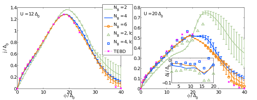
Figure 3: (Color online) Current $j$ vs. voltage $\phi$ for the model (1) with tight-binding leads and on-site interaction $U=12\,\Delta_{0}$ (left) and $U=20\,\Delta_{0}$ (right). Results for three different auxiliary systems with $N_{B}\in\{2,4,6\}$ are displayed and compared with reference data from TEBD (magenta dotted and $\times$). Nuss et al. (2013) We plot the averaged mean values connected by lines together with error bars determined according to Sec. III.1 and App. B. The additional data marks for $U=20\,\Delta_{0}$ are as follows: The circles for $N_{B}=6$ display $j(\phi)$ when considering the absolute minimum in the fit (12). $N_{B}=2,\mathrm{lc}$ and $N_{B}=4,\mathrm{lc}$ present the results of a linear correction of the current values of the absolute minima as described in App. C. The inset displays the difference $\Delta j$ of the calculated currents to the TEBD results.

When following the absolute minimum of the cost function Eq. (12) as a function of some external parameter, such as, e.g., the bias voltage $\phi$, spurious discontinuities appear due to the fact that local minima cross each other. This occurs for large bias voltages and large $U$, and/or small $N_{B}$, for which the approach is more challenging. An example for such a situation is shown in Fig. 2 for the case $N_{B}=4$, when comparing the hybridization functions just before and after such a crossing, i.e. for $\phi=27\,\Delta_{0}$ and $\phi=28\,\Delta_{0}$. Even though the changes in the exact hybridization function are only minor, $\underline{\Delta}_{\text{aux}}(\omega)$ displays a considerable difference. The influence of this spurious effect on observable quantities is shown in Fig. 3 (right panel, orange circles) for a different parameter set of $N_{B}=6$ at around $\phi_{c}=33\,\Delta_{0}$. The artificial discontinuity in the current is caused by the shift of spectral weight in $\underline{\Delta}_{\text{aux}}(\omega)$.

To deal with these discontinuities, we adopt a scheme which is suitable for obtaining a continuous dependence of observables on external parameters and in addition, allows to estimate their uncertainties (see Fig. 3). We first identify a set of local minima of the cost function Eq. (12), obtained by a series of minimum searches starting with random initial values. These local minima are then used to calculate an average and variance of physical quantities, such as the current. We consider the distribution of local minima with a Boltzmann weight associated with an artificial “temperature”, whereby the value of the cost function Eq. (12) is the associated “energy”. This artificial temperature for the Boltzmann weight is chosen in such a way, that the averaged spectral weight of the hybridization function as a function of $\phi$ is as smooth as possible. Details are outlined in App. B. A possible pitfall however is, that physical discontinuities, i.e., real phase transitions could be overlooked. It is thus compulsory to additionally investigate the results for the absolute minima and for different bath setups carefully. This approach has a certain degree of arbitrariness. However, we point out that it only affects regions with large error bars in Fig. 3, i.e. large $\phi$ and large $U$ for which also other techniques are less accurate.

III.2 Current voltage characteristics

After evaluating the interacting impurity Green’s function of the physical system according to (5) with the self energy evaluated in Sec. II.4, we are able to determine the steady-state current. This is done with the help of the Meir-Wingreen expression Meir and Wingreen (1992); Haug and Jauho (1998); Jauho (2006) in its symmetrized form, where we have already summed over spin

$$j =i\int\limits_{-\infty}^{\infty}\frac{d\omega}{2\pi}\left(\left(\gamma_{L}(\omega)-\gamma_{R}(\omega)\right)G^{<}(\omega)\right.$$ (45)

$$+\left.\left(p_{\text{F},L}(\omega)\gamma_{L}(\omega)-p_{\text{F},R}(\omega)\gamma_{R}(\omega)\right)\left(G^{R}(\omega)-G^{A}(\omega)\right)\right)\,\mbox{,}$$

$\gamma_{\lambda}(\omega)=-2|t^{\prime}_{\lambda}|^{2}\Im{m}\,(g_{\lambda}^{R}(\omega))$ are the “lead self-energies“ and $p_{\text{F},\lambda}(\omega)=p_{\text{F}}(\omega-\mu_{\lambda})$ denotes the Fermi distribution of lead $\lambda$ with chemical potential $\mu_{\lambda}$.

To quantify the accuracy of the method we compare the results for the current voltage characteristics with quasi exact reference data from TEBD. Nuss et al. (2013) We find very good agreement for interaction strength $U<12\,\Delta_{0}$. Since in this paper we want to benchmark the approach in “difficult” parameter regimes, in the following, we will discuss $U\gtrsim 12\Delta_{0}$ only. In Fig. 3 we display data for $U=12\,\Delta_{0}$ and $U=20\,\Delta_{0}$. The data points and error bars shown are obtained by using the averaging scheme as described in App. B. For the universal physics at small and medium bias voltages $\phi\lesssim 20\,\Delta_{0}$, the current as a function of the auxiliary system size ($N_{B}\in\{2,4,6\}$) converges rapidly to the expected result. The convergence is even monotonic in a broad region of the parameter space. The zero bias response is linear for all $N_{B}$ and approaches the results expected from the Friedel sum rule Cyril (1997) $j(\phi=0^{+})=2\frac{e^{2}}{h}\phi$ quickly for increasing $N_{B}$. For $U=12\,\Delta_{0}$ already the $N_{B}\gtrsim 4$ results yield a good reproduction of the current in this bias regime. For $U=20\,\Delta_{0}$ and $\phi\gtrsim 20\,\Delta_{0}$ a larger difference between the $N_{B}=4$ and $N_{B}=6$ results is observed. Notice that also other available methods do not yield a satisfactory result in this parameter regime. In the lead dependent high bias regime the fit becomes more challenging and large variances appear in the calculated quantities. This indicates the presence of many competing local minima with similar values for the cost function whose value tends to increase with increasing $\phi$. For $\phi\geq 40\,\Delta_{0}$ the densities of states of the left and the right contact do not overlap anymore and the current has to vanish. This limit cannot be exactly reproduced by the proposed approach due to spurious long-range Lorentzian tails present in the auxiliary Markovian environment. Nevertheless, $j(\phi=40\,\Delta_{0})$ approaches zero as one increases the number of bath sites. This holds true for quantities obtained at the absolute minimum of the cost function as well as for averaged ones.

To extrapolate our results to larger $N_{B}$, a scheme for linear corrections is discussed in App. C. Data for $N_{B}=2,\mathrm{lc}$ and $N_{B}=4,\mathrm{lc}$, whereby “lc” denotes “linear correction”, is shown in Fig. 3. For large $U=20\,\Delta_{0}$ and small to medium bias voltages $\phi\lesssim 20\,\Delta_{0}$, a solid improvement towards the TEBD reference values is observed (see inset Fig. 3). Correction ratios $r$ (see App. C) close to one indicate a good applicability of the linear correction scheme. We find on average $r\approx 0.75$ for $\phi\lesssim 20\,\Delta_{0}$ ($N_{B}=2,\mathrm{lc}$ and $N_{B}=4,\mathrm{lc}$). In the high bias regime, however, the linear correction cannot be applied with large magnitude and $r$ drops below $0.5$ for $N_{B}=2,\mathrm{lc}$. Nevertheless, the calculation of the effective, auxiliary hybridization function $\underline{\Delta}_{\text{aux},r}(\omega)$ as described in App. C, successfully avoids an ”over-correction” of the current values and automatically allows one to estimate the reliability of the results.

Judging from the larger uncertainty from the averaging procedure and the strong effects of the linear corrections, we conclude that the high bias regime is more sensitive to the details of the fitted, auxiliary hybridization function. The universal low and medium bias regime are however very well reproduced even with a small number of auxiliary bath sites.

III.3 Non-equilibrium spectral function

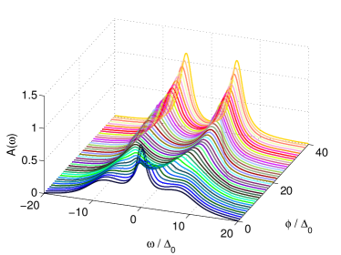
(a)

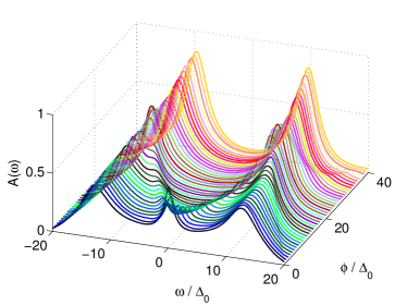
(b)

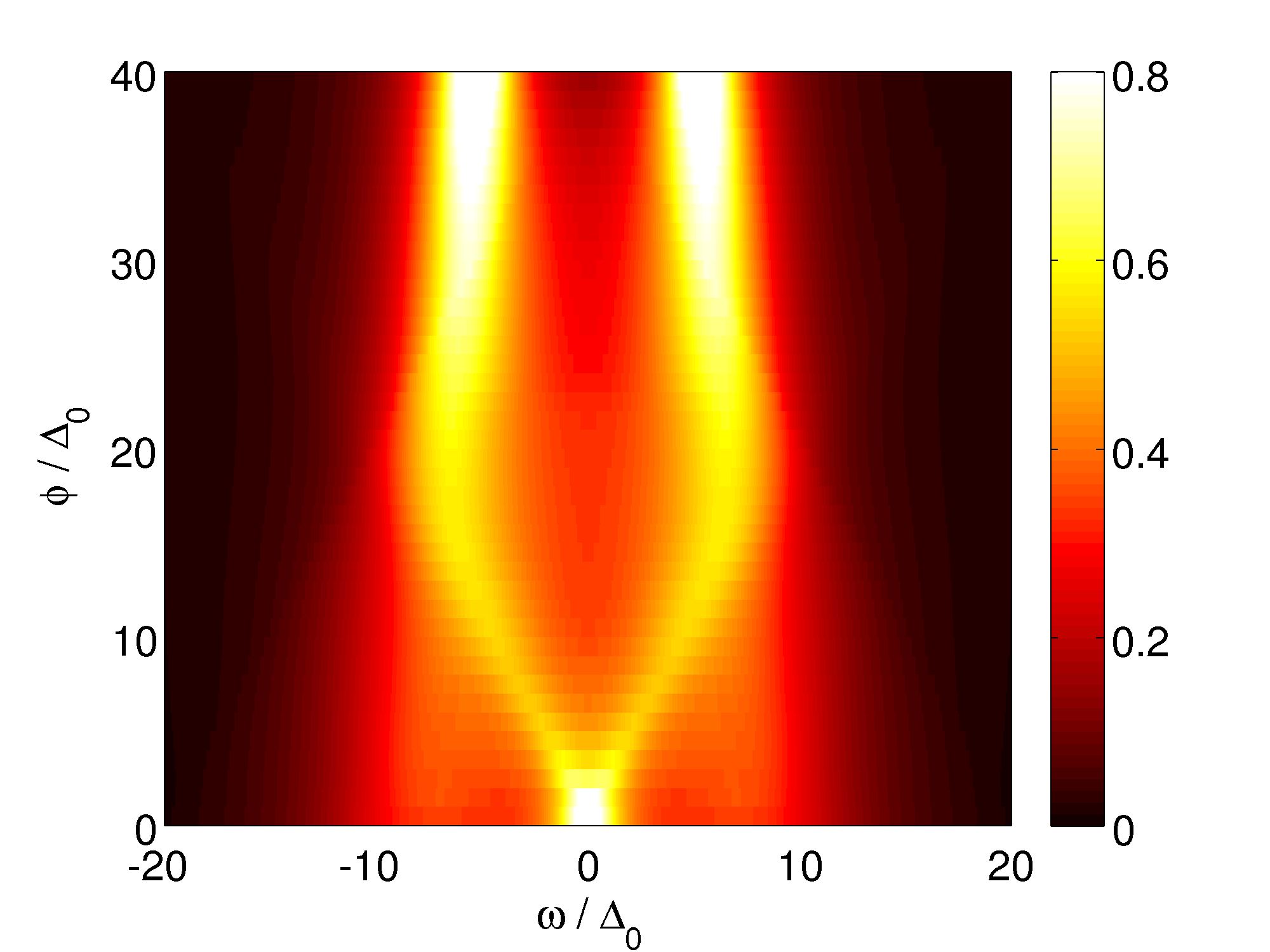
(c)

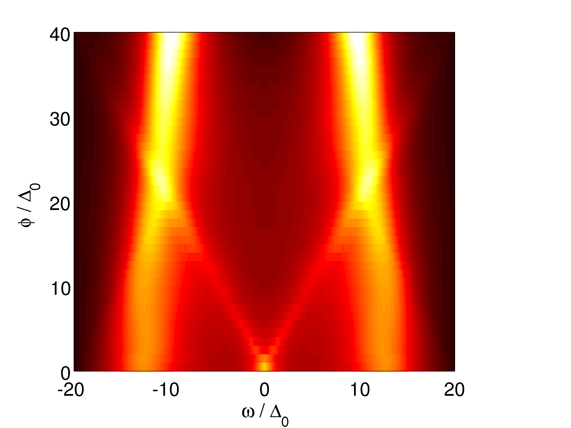
(d)

Figure 4: (Color online) Single particle spectral function at the impurity evaluated for $N_{B}=6$, different bias voltages $\phi$ and $U=12\,\Delta_{0}$ (left) and $U=20\,\Delta_{0}$ (right). Data is obtained according to Sec. III.1 and App. B. Other parameters are as in Fig. 3.

The bias-dependent single particle spectral function is evaluated from the physical steady state Green’s function of the impurity $A(\omega)=-\frac{1}{\pi}\Im{m}\,(G^{R}(\omega))$. Results obtained using $N_{B}=6$ for $U=12\,\Delta_{0}$ and $U=20\,\Delta_{0}$ are presented for the whole bias range of interest in Fig. 4. Data for $N_{B}=4$ are similar but here the Kondo physics cannot be reproduced as accurately as in the case of $N_{B}=6$. Our approach does preserve the local charge density $\langle n_{f}\rangle=\sum\limits_{\sigma}\frac{1}{2}+\frac{1}{2}\int\limits_{-\infty}^{\infty}\frac{d\omega}{2\pi}\Im{m}\,(G^{K}(\omega))=1$ and magnetization $\langle m_{f}\rangle=0$ as well as the spectral sum rule. Negele and Orland (1988)

The presented method reproduces qualitatively correctly also the equilibrium physics at $\phi=0$, since $A(\omega)$ displays a Kondo resonance at $\omega=0$ and two Hubbard satellites at the approximate positions $\omega\approx\pm U/2$. This renders the application to equilibrium DMFT problems an interesting perspective. The width and magnitude of the Kondo resonance is discussed in comparison with (S)NRG data in Sec. III.3.1.

Upon increasing the bias voltage, the Kondo resonance splits up and two excitations are observed at the energies of the Fermi levels of the leads. De Franceschi et al. (2002); Leturcq et al. (2005); Nuss et al. (2012) For $U=12\,\Delta_{0}$, the splitted resonances merge into the Hubbard bands at approximately $\phi\approx 15\,\Delta_{0}$ and cannot be clearly identified thereafter. In contrast, in the case of $U=20\,\Delta_{0}$ the resonances overlap with the Hubbard satellites and can still be observed in the spectrum $A(\omega)$ at higher voltages. Calculations with increasing $U$ in the high bias regime $\phi\approx 40\,\Delta_{0}$ have shown the consistency of this effect and that a minimum value of $U\approx 15\,\Delta_{0}$ is needed in order for the resonances at the Fermi energies to be perceptible after having crossed the Hubbard bands.

III.3.1 Comparison with scattering states numerical renormalization group

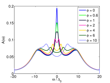
Figure 5: (Color online) Single particle spectral function for a constant DOS of the leads Eq. (3), with $D_{\text{WB}}=20\,\Delta_{0}$ and $U=16\,\Delta_{0}$ and different bias voltages $\phi$ (in units of $\Delta_{0}$). Results are obtained for $N_{B}=6$ and at the absolute minimum of Eq. (12). For a comparison with SNRG Anders (2008) (Fig. 2a therein), note that their $\Gamma=2\,\Delta_{0}$.

We compare the computed spectral functions with results obtained by means of SNRG. Anders (2008) For this purpose, we use a flat DOS Eq. (3) for the leads, as in Ref. Anders, 2008. Focusing on the low bias regime and $N_{B}=6$, the obtained spectral functions are depicted in Fig. 5. Compared with SNRG, our results do not achieve the same accuracy in the low energy domain, i.e. in the vicinity of $\omega\approx 0$. However, our data provides a better resolution at higher energies. When inspecting the Kondo peak in the equilibrium case $\phi=0$, our results do not fully fulfill the Friedel sum rule. Cyril (1997); Langer and Ambegaokar (1961); Langreth (1966) Depending on parameters the height of the Kondo resonance is underestimated. This is due to the fact that the imaginary part of the self-energy at $\omega=0$ has a small finite value which is due to the Lorentzian tails of the Markovian environment.

The resolution does not suffice to tell whether a two or a three peak structure is present for very low bias voltages $\phi\lesssim 2\,\Delta_{0}$. Nevertheless, one can say that the higher bias regime $\phi>4\,\Delta_{0}$ is resolved more accurately and one is able to clearly distinguish the excitations at the Fermi energies of the contacts from the Hubbard satellites. The observed linear splitting is consistent with experiments on nanodevices. Leturcq et al. (2005); De Franceschi et al. (2002) Within second-order Keldysh PT Fujii and Ueda (2003) and QMC results Mühlbacher et al. (2011) the resonance does not split but is suppressed only. In fourth-order and in NCA it splits into two, which are located near the chemical potentials of the two leads. Fujii and Ueda (2003) Other methods yield a splitting with features slightly different in details: real-time diagrammatics, König et al. (1996) VCA, Nuss et al. (2012) imaginary potential QMC Dirks et al. (2013b) or scaling methods. Rosch et al. (2003)

Overall, a good qualitative agreement with the SNRG results is achieved which underlines the reliability of the calculated spectral functions.

III.3.2 Linear correction of Green’s functions

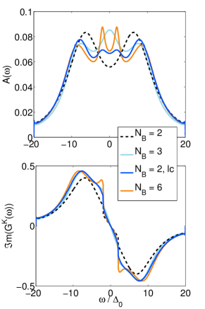
(a)

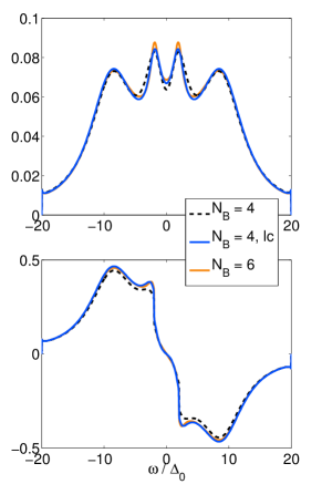
(b)

Figure 6: (Color online) Effects of the linear corrections of the Green’s functions according to Sec. C (solid blue lines). The dashed lines indicate the uncorrected $\underline{G}(\omega)$ with the same $N_{B}$, while solid orange and light blue lines display results for larger $N_{B}$ for comparison. Results are shown for a constant lead DOS Eq. (3) with $D_{\text{WB}}=20\,\Delta_{0}$, $U=16\,\Delta_{0}$ and $\phi=4\,\Delta_{0}$.

Here we consider the effect of a linear correction of the Green’s functions, as outlined in App. C. In the left panels (right panels) of Fig. 6, we show data for $N_{B}=2$ ($N_{B}=4$) including linear corrections ($r=1$) for a high interaction strength in the low bias regime. We benchmark to data obtained using $N_{B}=6$ without corrections.

For $N_{B}=2$ without linear corrections, the spectral function of the auxiliary system does not feature excitations at the Fermi energies of the contacts ($\omega=\pm 2\,\Delta_{0}$), which are present in the $N_{B}=6$ data. Also the spectra appear washed out. The linearly corrected result, however, features not only the two resonances at the appropriate energies but also the shoulders present in the reference data. Again in the Keldysh Green’s function a large correction towards the more accurate $N_{B}=6$ results is observed. To highlight the fact that the improvement of the linear correction is not only due to the inclusion of one additional bath site, also a calculation for an auxiliary system with $N_{B}=3$ is shown. Evidently, the $N_{B}=3$ spectral function exhibits a large weight at low frequencies, but, the resolution is rather low and only a single, smeared out peak at $\omega=0\,\Delta_{0}$ is observed. It clearly does not account for the splitting of the Kondo resonance.

For $N_{B}=4$, a similar enhancement is found. Clearly the size of the corrections is much smaller. Especially in the Keldysh component, the Green’s function for $N_{B}=6$ and for the corrected $N_{B}=4$ system nearly coincide. In general, the difference between the $N_{B}=6$ and the $N_{B}=4$ calculations (raw and corrected) are quite small, so that the presented spectral functions in Fig. 5 for larger values of $\phi\lesssim 12\,\Delta_{0}$ can be assumed to be quite accurate.

Overall, the linear correction enables a vast improvement in the universal low and medium bias regime for all $U$, which becomes especially important for large $U$. For large bias voltages, when lead band effects become prominent, the linear correction is more challenging (see also Sec. III.2).

IV Conclusions

We have presented a numerical approach to study correlated quantum impurity problems out of equilibrium. Arrigoni et al. (2013) The auxiliary master equation approach presented here is based on a mapping of the original Hamiltonian to an auxiliary open quantum system consisting of the interacting impurity coupled to bath sites as well as to a Markovian environment. The dynamics of the auxiliary open system are controlled by a Lindblad master equation. Its parameters are determined by a fit to the impurity-environment hybridization function. This has many similarities to the procedure used for the exact-diagonalization dynamical mean field theory impurity solver, but has the advantage that one can work directly with real frequencies, which is mandatory for non-equilibrium systems.

We have illustrated how the accuracy of the results can be estimated, and systematically improved by increasing the number of auxiliary bath sites. A scheme to introduce linear corrections has been devised. We presented in detail how the non-equilibrium Green’s functions of the correlated open quantum system are obtained by making use of non-hermitian Lanczos diagonalization in a super-operator space. These techniques make the whole method fast and efficient as well as particularly suited as an impurity solver for steady state dynamical mean field theory. Arrigoni et al. (2013)

In this work we have applied the approach to the single impurity Anderson model, which is one of the paradigmatic quantum impurity models. We have analyzed in detail the systematic improvement of the current-voltage characteristics as a function of the number of auxiliary bath sites. Already for four auxiliary bath sites, results show a rather good agreement with quasi exact data from time evolving block decimation Nuss et al. (2013) in the low and medium bias regime. In the high bias regime, the current deviates from the expected result with increasing interaction strength. However, we have shown how to estimate the reliability of the data from the deviation of the hybridization functions and how results can be corrected to linear order in this deviation. The impurity spectral function obtained in our calculation features a linear splitting of the Kondo resonance as a function of bias voltage. Good agreement with data from scattering state numerical renormalization group Anders (2008) was found.

Applications of the presented method to multi-orbital correlated impurities or correlated clusters is in principle straightforward, although numerically more demanding. Such systems are themselves of interest as models for transport through molecular or nanoscopic objects and as solvers for non-equilibrium cluster dynamical mean field theory. In this case, a larger number of auxiliary sites might be necessary to obtain a good representation of the various hybridization functions. For this situation, one should use numerically more efficient methods to solve for larger correlated open quantum systems, such as matrix product states and density matrix renormalization group, possibly combined with stochastic wave-function approaches, Dalibard et al. (1992); Daley et al. (2009); Prosen and Znidaric (2009), sparse polynomial space, Alvermann and Fehske (2009); Weisse et al. (2006) or configuration interaction approaches. Sherrill and III (1999) A more accurate determination of low-energy, and possibly critical properties might be achieved by a combination with renormalization group iteration schemes, similar to the numerical renormalization group. Work along these lines is in progress.

Although we have presented results for the steady state, where the method is most efficient, also extensions to time dependent phenomena provide an interesting and feasible perspective. While other approaches, such as time-dependent density matrix renormalization group, White and Feiguin (2004) or quantum Monte Carlo, Eckstein et al. (2009) are certainly more accurate at short times, the present approach could be used to estimate directly slowly-decaying modes by inspecting the behavior of the low-lying spectrum of the Lindblad operator.

Appendix A Numerical calculation of the auxiliary interacting Green’s function

In this section we present details of the numerical evaluation of the auxiliary Green’s function, as described in Sec. II.4.2. We focus on large Hilbert spaces for which a sparse-matrix approach is mandatory.

To determine the steady state, which is the right-sided eigenstate of ${\hat{L}}$ with eigenvalue zero, one can make use of a shift-and-invert Arnoldi procedure. Saad (2011); Arbenz (2012); Bai et al. (1987); Knap et al. (2011b) The spectrum of ${\hat{L}}$ Eq. (42) has the property that $\Im{m}\,(\ell_{n})<0$ for all eigenvalues $\ell_{n}$ (except the steady state $\ell_{0}=0$). Therefore, given a small shift $s>0$, the eigenvector of $({\hat{L}}-is\hat{11})^{-1}$ with the largest eigenvalue is the steady state. Since ${\hat{L}}$ is non-hermitian, the three term recurrence of the ordinary Lanczos scheme Lanczos (1951) does not apply, and one has to resort to an Arnoldi scheme instead. To construct the corresponding Krylov space, a system of equations $({\hat{L}}-is\hat{11})\mathinner{|{\tilde{\phi}_{n+1}}\rangle}=\mathinner{|{\phi_{n}}\rangle}$ has to be solved in each step. For the problem at hand we found that this can be done most efficiently by combining a stabilized biconjugate gradient method with an incomplete LU-decomposition as preconditioner. Saad (2003); Barrett et al. (1994) Despite using sparse matrix methods the memory requirements of this approach are rather high compared to the schemes presented below.

A second possible route to determine the steady state $\mathinner{|{\rho_{\infty}}\rangle}$ is to perform an explicit time evolution. For unitary time evolutions a well-established method relies on the Lanczos scheme to construct an approximate time evolution operator. Park and Light (1986) Such an approach can be adapted to the non-unitary case by using a two-sided Lanczos scheme (see below), or also by employing an Arnoldi procedure. Knap et al. (2011b) Since ${\hat{L}}$ is non-hermitian, one can equally well use a simpler backward or forward Euler scheme Press et al. (2007) to discretize the non-unitary time evolution operator. These approaches may not yield a highly accurate time evolution of $\mathinner{|{\rho(t)}\rangle}$, but can nevertheless determine the steady state within a moderate number of steps. As for the shift-and-invert approach above, to solve the implicit update of $\mathinner{|{\rho(t_{n+1})}\rangle}$ at time step $t_{n}$ in the case of the backward Euler, a biconjugate gradient routine has proven to be effective. For the forward time-integration a Runge Kutta method of second order is sufficient, with the great advantage that only matrix-vector multiplications are needed, which reduces memory requirements. In practice, for the considered cases it was found that for not too large systems ($N_{B}<6$) the shift-and-invert Arnoldi procedure is best suited, whereas a forward time-integration is advantageous for the case $N_{B}=6$.

Once the steady state is determined, Green’s functions can be effectively calculated by employing a two-sided Lanczos scheme. Saad (2011); Bazaliy et al. (1997); Gutknecht (1990, 1999); Freund et al. (1993); Parlett et al. (1985) We therefore express the right- and left-sided eigenvectors of ${\hat{L}}$ in Eq. (43) in a Krylov space basis

$$\mathinner{|{R_{n}}\rangle} =\sum_{k}U_{kn}\mathinner{|{\phi_{R}^{k}}\rangle}\,\mbox{,}\quad\mathinner{\langle{L_{n}}|}=\sum_{k}\left(U^{-1}\right)_{nk}\mathinner{\langle{\phi_{L}^{k}}|}\,\mbox{.}$$

Here, we have omitted the $N_{\sigma}-\tilde{N}_{\sigma}$ symmetry sector index for the sake of clarity. The biorthogonal Lanczos vectors

$$\mathinner{\langle{\phi_{L}^{k}|\phi_{R}^{k^{\prime}}}\rangle} =\delta_{kk^{\prime}}\,\mbox{,}$$

are determined by the three term recurrence

$$\mathinner{|{\phi_{R}^{n+1}}\rangle} =\frac{1}{c_{n+1}}\left({\hat{L}}\mathinner{|{\phi_{R}^{n}}\rangle}-e_{n}\mathinner{|{\phi_{R}^{n}}\rangle}-k_{n}\mathinner{|{\phi_{R}^{n-1}}\rangle}\right)\,\mbox{,}$$

$$\mathinner{\langle{\phi_{L}^{n+1}}|} =\frac{1}{c_{n+1}^{*}}\left(\mathinner{\langle{\phi_{L}^{n}}|}{\hat{L}}-e_{n}\mathinner{\langle{\phi_{L}^{n}}|}-k_{n}^{*}\mathinner{\langle{\phi_{L}^{n-1}}|}\right)\,\mbox{,}$$

with

$$e_{n} =\mathinner{\langle{\phi_{L}^{n}}|}{\hat{L}}\mathinner{|{\phi_{R}^{n}}\rangle}\,\mbox{,}$$

$$k_{n} =\mathinner{\langle{\phi_{L}^{n-1}}|}{\hat{L}}\mathinner{|{\phi_{R}^{n}}\rangle}=\left(\mathinner{\langle{\phi_{L}^{n}}|}{\hat{L}}\mathinner{|{\phi_{R}^{n-1}}\rangle}\right)^{*}\,\mbox{,}$$

and a normalization constant $c_{n}$ such that $\mathinner{\langle{\phi_{L}^{n}|\phi_{R}^{n}}\rangle}=1$. One has a certain degree of freedom in the choice of $c_{n}$ and $k_{n}$ due to the relation $k_{n}^{*}=c_{n}$, which is fulfilled for example by $k_{n}=k_{n}^{*}=c_{n}$.

In the Krylov basis, ${\hat{L}}$ takes on a tridiagonal form $T_{nm}=\mathinner{\langle{\phi_{L}^{n}}|}{\hat{L}}\mathinner{|{\phi_{R}^{m}}\rangle}$ with the matrix elements $T_{nn}=e_{n}$, $T_{n-1n}=k_{n}$ and $T_{nn-1}=k_{n}^{*}$. When $n+1$ becomes as large as the degree of the minimal polynomial of ${\hat{L}}$, the eigenvalues and eigenvectors of $T$ represent those of ${\hat{L}}$. Gutknecht (1990); Saad (2011) If one truncates the Krylov basis, this statement holds still approximately true, especially for the largest eigenvalues in magnitude. Analogous to the hermitian case, Weikert et al. (1996) an exponential convergence of the eigenspectrum of $T$ towards the one of ${\hat{L}}$ is observed, which is of particular importance for the calculation of Green’s functions. A peculiarity of the two-sided Lanczos scheme is, that not every Krylov subspace guarantees that $\Im{m}\,(\ell_{n})<0$ for all eigenvalues $\ell_{n}$ of $T$. In order to obtain the appropriate pole structure for the estimated Green’s functions, one has to check $\Im{m}\,(\ell_{n})<0$ together with convergence criteria. In cases in which $\Im{m}\,(\ell_{n})<0$ cannot be fulfilled exactly, it has to be ensured at least that the corresponding weights of these eigenvalues are negligible.

For the calculation of the Green’s functions needed here it is convenient to choose appropriate initial vectors, which are in the case of the greater Green’s function (43)

$$\mathinner{|{\phi_{R}^{0}}\rangle} =\frac{1}{c_{0}}\left(d^{\dagger}_{f}\mathinner{|{\rho_{\infty}}\rangle}\right)\,\mbox{,}\quad\mathinner{\langle{\phi_{L}^{0}}|}=\frac{1}{c_{0}^{*}}\left(\mathinner{\langle{I}|}d_{f}^{\phantom{{\dagger}}}\right)\,\mbox{.}$$

When denoting by $\ell_{n}$ and $U_{k,n}$ the eigenvalues and right-sided eigenvectors of $T$, respectively, Eq. (43) can be cast into the form

$$G^{>}(\omega) =\sum_{n,k,k^{\prime}}\frac{U_{kn}{U}^{-1}_{nk^{\prime}}}{\omega-\ell_{n}}\mathinner{\langle{I}|}d_{f}^{\phantom{{\dagger}}}\mathinner{|{\phi_{R}^{k}}\rangle}\mathinner{\langle{\phi_{L}^{k^{\prime}}}|}d^{\dagger}_{f}\mathinner{|{\rho_{\infty}}\rangle}$$

$$-\sum_{n,k,k^{\prime}}\frac{\left(U_{kn}{U}^{-1}_{nk^{\prime}}\right)^{*}}{\omega-\ell_{n}^{*}}\left(\mathinner{\langle{I}|}d_{f}^{\phantom{{\dagger}}}\mathinner{|{\phi_{R}^{k}}\rangle}\mathinner{\langle{\phi_{L}^{k^{\prime}}}|}d^{\dagger}_{f}\mathinner{|{\rho_{\infty}}\rangle}\right)^{*}$$

$$=\left|c_{0}\right|^{2}\sum_{n}\frac{U_{0n}{U}^{-1}_{n0}}{\omega-\ell_{n}}-\left|c_{0}\right|^{2}\sum_{n}\frac{\left(U_{0n}{U}^{-1}_{n0}\right)^{*}}{\omega-\ell_{n}^{*}}\,\mbox{.}$$

Appendix B Averaging scheme for multiple local minima

This section contains details on the approach we used to determine the artificial ”temperature“ for the Boltzmann weights as described in Sec. III.1. We consider the situation that a set of local minima for which Eq. (12) becomes stationary is known. Let us specify by $\mathbf{a}_{y}(\phi)$ the vector of parameters $\{E_{\mu\nu},\Gamma_{\mu\nu}^{(\kappa)}\}_{y}$ corresponding to one certain local minimum for a set of model parameters, labeled by $y$. In order to quantify the spectral weight distribution of the corresponding hybridization function $\underline{\Delta}_{\text{aux}}(\omega;\mathbf{a}_{y}(\phi))$, we define

$$m_{2}^{R}(\mathbf{a}_{y}(\phi)) =\int\limits_{-\omega_{c}}^{\omega_{c}}\Im{m}\,(\Delta^{R}_{\text{aux}}(\omega;\mathbf{a}_{y}(\phi)))\,\omega^{2}d\omega\,\mbox{,}$$

$$m_{3}^{K}(\mathbf{a}_{y}(\phi)) =\int\limits_{-\omega_{c}}^{\omega_{c}}\Im{m}\,(\Delta^{K}_{\text{aux}}(\omega;\mathbf{a}_{y}(\phi)))\,\omega^{3}d\omega\,\mbox{,}$$

which are similar to the second and third moment of $\Delta^{R}_{\text{aux}}$ and $\Delta^{K}_{\text{aux}}$, respectively. For the Keldysh component a definition analogous to the first moment would yield the desired information as well but the choice above has been found to be more sensitive to details of $\Delta^{K}_{\text{aux}}$. The value of the corresponding cost function $\chi(\mathbf{a}_{y}(\phi))$ of the $y$-th minimum is used as an artificial ”energy“ and enables one to define weights when making use of Boltzmann’s statistic

$$P_{y}(\phi,\beta) =\frac{1}{Z}e^{-\beta\chi(\mathbf{a}_{y}(\phi))}\,\mbox{,}$$

where we introduced an artificial ”temperature“ $\beta^{-1}$. For each bias voltage separately, we are then able to calculate averaged quantities

$$\overline{m_{2}^{R}}(\phi,\beta) =\sum\limits_{y}P_{y}(\phi,\beta)m_{2}^{R}(\mathbf{a}_{y}(\phi))\,\mbox{,}$$

as well as $\overline{m_{3}^{K}}(\phi,\beta)$ and $\overline{\chi}(\phi,\beta)$ in an analogous manner. The quantities $\overline{m_{2}^{R}}(\phi,\beta)$ and $\overline{m_{3}^{K}}(\phi,\beta)$ provide an estimate of the center of the spectral weight for the averaged set of hybridization functions for each bias voltage $\phi$.

Our goal is that these quantities vary in a smooth way when changing the bias voltage. To achieve this, we employ a minimum curvature scheme, Press et al. (2007) meaning that we optimize the function

$$v_{c}(\beta) =\int\limits_{0}^{\phi_{max}}\left\{w^{R}\left|\frac{\partial^{2}}{\partial\phi^{2}}\overline{m_{2}^{R}}(\phi,\beta)\right|^{2}+w^{K}\left|\frac{\partial^{2}}{\partial\phi^{2}}\overline{m_{3}^{K}}(\phi,\beta)\right|^{2}\right.$$

$$\left.+w^{\chi}\left|\frac{\partial^{2}}{\partial\phi^{2}}\overline{\chi}(\phi,\beta)\right|^{2}\right\}d\phi\,\mbox{,}$$

with respect to $\beta$. This determines the optimal artificial ”temperature“, which ensures that the averaged cost function as well as the averaged spectral weight are as smooth functions of $\phi$ as possible, given the set of calculated minima $\{\mathbf{a}_{y}(\phi)\}$. As in many optimization problems, an arbitrariness exists in the definition of the quantities $\overline{m_{2}^{R}}(\phi,\beta)$ and $\overline{m_{3}^{K}}(\phi,\beta)$, as well as in choosing the values of the weights $w^{R}$, $w^{K}$ and $w^{\chi}$. In our case all of the weights were chosen to be equal to one in units of $t$.

An improvement of the results, to a certain degree at least, could be expected when making use of extensions like a bias-dependent $\beta(\phi)$. This has not been considered in the present work since already a single variable $\beta$ provided quite smooth observables. As mentioned in the main text, in any case, it is obligatory to examine besides the averaged results also the ones for the absolute minima and/or for different averaging schemes, in order to avoid that physical discontinuities are averaged out. We stress that this approach has to be taken with due care, since it is in some aspects arbitrary. However, it is useful to give an estimate of the error of the calculation, and can certainly identify regions in parameter space where the error is negligible small.

Appendix C Linear corrections

In this section, we present a scheme to correct physical quantities up to linear order in the difference foo (l)

$$\underline{D}(\omega) =\underline{\Delta}_{ex}(\omega)-\underline{\Delta}_{\text{aux}}(\omega)\,\mbox{,}$$

between the auxiliary and the exact hybridization functions. Although $\underline{D}(\omega)$ decreases rapidly with increasing number of auxiliary bath sites $N_{B}$, the size of the Hilbert space also increases exponentially with $N_{B}$. This poses a clear limit to the maximum value of $N_{B}$.

The idea is based on the fact that each physical quantity $O[\underline{\Delta}]$ is a functional of $\underline{\Delta}(\omega)$. Its exact value is, thus, obtained as $O[\underline{\Delta}_{ex}]$. For a finite $N_{B}$ there will always be a nonzero value of $\underline{D}(\omega)$ at some energies, so we will always obtain an approximate value $O[\underline{\Delta}_{\text{aux}}]$. A linear correction can be obtained by evaluating numerically the functional derivative of $O[\underline{\Delta}]$. Strictly speaking, considering that only $\Im{m}\,(\Delta^{R}(\omega))$ and $\Im{m}\,(\Delta^{K}(\omega))$ are independent functions, $O$ is a functional $O[\Im{m}\,(\Delta^{R}),\Im{m}\,(\Delta^{K})]$. Suppose one knows the functional derivatives

$$\frac{\delta O[\underline{\Delta}]}{\delta\Im{m}\,(\Delta^{\alpha}(\omega))}\,\mbox{,}\quad\quad \alpha\in\{R,K\}\,\mbox{,}$$

then to linear order in $\underline{D}(\omega)$

$$O[\underline{\Delta}_{ex}] \approx O[\underline{\Delta}_{\text{aux}}]$$ (46)

$$+r\sum_{\alpha\in\{R,K\}}\int\left.\frac{\delta O[\underline{\Delta}]}{\delta\Im{m}\,(\Delta^{\alpha}(\omega_{0}))}\right|_{\underline{\Delta}=\underline{\Delta}_{\text{aux}}}\Im{m}\,(D^{\alpha}(\omega_{0}))\ d\omega_{0}+\mathcal{O}(\underline{D}^{2})\,\mbox{,}$$

with $r=1$.

We evaluate the functional derivative numerically in the following way. One first evaluates $O[\underline{\Delta}_{\text{aux}}]$ at the optimum $\underline{\Delta}_{\text{aux}}(\omega)$. Then $O$ is evaluated at a “shifted” $\Im{m}\,(\Delta^{\alpha}(\omega))$, obtained by adding a delta function peaked around a certain energy $\omega_{0}$

$$\delta_{\omega_{0}}(\omega) \equiv\delta(\omega-\omega_{0})\,\mbox{,}$$

multiplied by a small coefficient $\epsilon$. The functional derivatives are then approximated linearly, by making use of the equations

$$\frac{\delta O[\underline{\Delta}]}{\delta\Im{m}\,(\Delta^{R}(\omega_{0}))}\pm 2\frac{\delta O[\underline{\Delta}]}{\delta\Im{m}\,(\Delta^{K}(\omega_{0}))}$$ (47)

$$\approx\frac{1}{\epsilon}\left(O[\Im{m}\,(\Delta^{R}),\Im{m}\,(\Delta^{K})]\right.$$

$$-\left.O[\Im{m}\,(\Delta^{R})-\epsilon\delta_{\omega_{0}},\Im{m}\,(\Delta^{K})\mp 2\epsilon\delta_{\omega_{0}}]\right)\,\mbox{,}$$

which become exact in the $\epsilon\to 0$ limit.

A (quasi) delta-peak correction $\epsilon\delta_{\omega_{0}}$ to $\Delta^{\alpha}(\omega)$ can be obtained by attaching an additional bath site ($N_{B}+1$) with on-site energy $E_{N_{B}+1,N_{B}+1}=\omega_{0}$ directly to the impurity site with a hopping $E_{N_{B}+1,f}=\sqrt{\epsilon/\pi}$. The sum of $\Gamma_{N_{B}+1,N_{B}+1}^{(1)}$ and $\Gamma_{N_{B}+1,N_{B}+1}^{(2)}$ is proportional to the width of $\delta_{\omega_{0}}$ and thus, should be taken as small as possible. In practice, one uses a discretization of the integration over $\omega_{0}$ in Eq. (46) and the width of the delta peaks has to be adjusted accordingly. Setting one of the components $\Gamma_{N_{B}+1,N_{B}+1}^{\kappa}$ to zero yields a peak in the Keldysh component with a coefficient $\pm 2\epsilon$, respectively, as used in Eq. (47).

Notice that the functional derivative Eq. (47) amounts to carrying out two many-body calculations for each point $\omega_{0}$ on a system with $N_{B}+1$ bath sites. However, it is not necessary to repeat the calculation for each physical quantity of interest. In the linearly corrected current values presented in Sec. III.2, a $\omega_{0}$ mesh of 200 points was used, whereby this number is likely to be reduced when optimizing the method.

Strictly speaking the coefficient $r$ in Eq. (46) should be $1$. However, for cases in which the linear correction is not small, this could produce an “over-correction”. In order to avoid this, we introduce a smaller ratio $r$ which is determined as follows: We evaluate the corrected self energy at each $\omega$ via Eq. (46) and $O=\underline{\Sigma}(\omega)$ with some value of $r<1$ and denote it $\underline{\Sigma}_{r}(\omega)$. We do the same for the Green’s function of the auxiliary system and denote it $\underline{G}_{r}(\omega)$. Using Equations (5) and (6) we now have an estimate of an effective $r$-dependent auxiliary hybridization function of the linearly corrected system via

$$\underline{\Delta}_{\text{aux},r}(\omega)\equiv\underline{g}^{-1}_{0}(\omega)-\underline{G}_{r}^{-1}(\omega)-\underline{\Sigma}_{r}(\omega)\,\mbox{.}$$

In principle, for $r=1$ this gives $\underline{\Delta}_{ex}(\omega)$ up to $\mathcal{O}(\underline{D}^{2})$. In practice, for finite $\underline{D}(\omega)$, one can introduce a cost function $\chi(r)$ analogous to Eq. (12) to minimize the difference $|\underline{\Delta}_{\text{aux},r}(\omega)-\underline{\Delta}_{ex}(\omega)|$ as a function of $r$. We checked that for the case in which the linear correction is a good approximation, the minimum occurs at $r=1$. If the minimum of $\chi(r)$ is situated at some value $r_{\text{min}}<1$ then one corrects also other physical quantities according to Eq. (46) with the same $r=r_{\text{min}}$.

Alternatively to the correction Eq. (46) discussed above, one can use the numerical functional derivative evaluated via Eq. (47) in order to estimate the sensitivity of the value of $O$ with respect to variations of $\Im{m}\,(\Delta^{\alpha}_{\text{aux}}(\omega))$ as a function of $\omega$ and $\alpha$. This is of use, in a second step, to adjust the weight function $W^{\alpha}(\omega)$ in Eq. (12), so that more sensitive $\omega$ regions acquire a larger weight.

References

- Hartmann et al. (2008) M. Hartmann, F. Brandão, and M. Plenio, Laser & Photonics Rev. 2, 527 (2008).
- Raizen et al. (1997) M. Raizen, C. Salomon, and Q. Niu, Phys. Today 50, 30 (1997).
- Jaksch et al. (1998) D. Jaksch, C. Bruder, J. I. Cirac, C. W. Gardiner, and P. Zoller, Phys. Rev. Lett. 81, 3108 (1998).
- Greiner et al. (2002) M. Greiner, O. Mandel, T. Esslinger, T. W. Hänsch, and I. Bloch, Nature 415, 39 (2002).
- Trotzky et al. (2008) S. Trotzky, P. Cheinet, S. Fölling, M. Feld, U. Schnorrberger, A. M. Rey, A. Polkovnikov, E. A. Demler, M. D. Lukin, and I. Bloch, Science 319, 295 (2008).
- Schneider et al. (2012) U. Schneider, L. Hackermuller, J. P. Ronzheimer, S. Will, S. Braun, T. Best, I. Bloch, E. Demler, S. Mandt, D. Rasch, et al., Nat Phys 8, 213 (2012).
- Iwai et al. (2003) S. Iwai, M. Ono, A. Maeda, H. Matsuzaki, H. Kishida, H. Okamoto, and Y. Tokura, Phys. Rev. Lett. 91, 057401 (2003).
- Cavalleri et al. (2004) A. Cavalleri, T. Dekorsy, H. H. W. Chong, J. C. Kieffer, and R. W. Schoenlein, Phys. Rev. B 70, 161102 (2004).
- Bonilla and Grahn (2005) L. L. Bonilla and H. T. Grahn, Rep. Prog. Phys. 68, 577 (2005).
- Zutic et al. (2004) I. Zutic, J. Fabian, and S. D. Sarma, Rev. Mod. Phys. 76, 323 (2004).
- Cuniberti et al. (2005) G. Cuniberti, G. Fagas, and K. Richter, Introducing Molecular Electronics (Springer, 2005), ISBN 3540279946.
- Smit et al. (2002) R. H. M. Smit, Y. Noat, C. Untiedt, N. D. Lang, M. C. van Hemert, and J. M. van Ruitenbeek, Nature 419, 906 (2002).
- Park et al. (2002) J. Park, A. N. Pasupathy, J. I. Goldsmith, C. Chang, Y. Yaish, J. R. Petta, M. Rinkoski, J. P. Sethna, H. D. Abruna, P. L. McEuen, et al., Nature 417, 722 (2002).
- Liang et al. (2002) W. Liang, M. P. Shores, M. Bockrath, J. R. Long, and H. Park, Nature 417, 725 (2002).
- Agrait et al. (2003) N. Agrait, A. L. Yeyati, and J. M. van Ruitenbeek, Physics Reports 377, 81 (2003).
- Venkataraman et al. (2006) L. Venkataraman, J. E. Klare, C. Nuckolls, M. S. Hybertsen, and M. L. Steigerwald, Nature 442, 904 (2006).
- Goldhaber-Gordon et al. (1998) D. Goldhaber-Gordon, J. Göres, M. A. Kastner, H. Shtrikman, D. Mahalu, and U. Meirav, Phys. Rev. Lett. 81, 5225 (1998).
- Kretinin et al. (2012) A. V. Kretinin, H. Shtrikman, and D. Mahalu, Phys. Rev. B 85, 201301 (2012).
- Mitra et al. (2006) A. Mitra, S. Takei, Y. B. Kim, and A. J. Millis, Phys. Rev. Lett. 97, 236808 (2006).
- Leggett et al. (1987) A. J. Leggett, S. Chakravarty, A. T. Dorsey, M. P. A. Fisher, A. Garg, and W. Zwerger, Rev. Mod. Phys. 59, 1 (1987).
- Cazalilla (2006) M. A. Cazalilla, Phys. Rev. Lett. 97, 156403 (2006).
- Rigol et al. (2008) M. Rigol, V. Dunjko, and M. Olshanii, Nature 452, 854 (2008).
- Nitzan and Ratner (2003) A. Nitzan and M. A. Ratner, Science 300, 1384 (2003).
- Anderson (1961) P. W. Anderson, Phys. Rev. 124, 41 (1961).
- Friedel (1956) J. Friedel, Can. J. Phys. 34, 1190 (1956).
- Clogston et al. (1962) A. M. Clogston, B. T. Matthias, M. Peter, H. J. Williams, E. Corenzwit, and R. C. Sherwood, Phys. Rev. 125, 541 (1962).
- Brenig and Schönhammer (1974) W. Brenig and K. Schönhammer, Zeitschrift für Physik 267, 201 (1974).
- Georges et al. (1996) A. Georges, G. Kotliar, W. Krauth, and M. J. Rozenberg, Rev. Mod. Phys. 68, 13 (1996).
- Cyril (1997) A. Cyril, The Kondo Problem to Heavy Fermions (Cambridge University Press, 1997), ISBN 0521599474.
- Vollhardt (2010) D. Vollhardt, in Lecture Notes on the Physics of Strongly Correlated Systems, edited by A. Avella and F. Mancini (AIP, New York, 2010), vol. 1297 of AIP Conf. Proc., pp. 339–403.
- Metzner and Vollhardt (1989) W. Metzner and D. Vollhardt, Phys. Rev. Lett. 62, 324 (1989).
- Kondo (1964) J. Kondo, Progress of Theoretical Physics 32, 37 (1964).
- Anderson (1970) P. W. Anderson, Journal of Physics C: Solid State Physics 3, 2436 (1970).
- Yosida and Yamada (1970) K. Yosida and K. Yamada, Progress of Theoretical Physics Supplement 46, 244 (1970).
- Yamada (1975a) K. Yamada, Progress of Theoretical Physics 53, 970 (1975a).
- Yosida and Yamada (1975) K. Yosida and K. Yamada, Progress of Theoretical Physics 53, 1286 (1975).
- Yamada (1975b) K. Yamada, Progress of Theoretical Physics 54, 316 (1975b).
- Schrieffer and Wolff (1966) J. R. Schrieffer and P. A. Wolff, Phys. Rev. 149, 491 (1966).
- Müller et al. (2013) S. Y. Müller, M. Pletyukhov, D. Schuricht, and S. Andergassen, Phys. Rev. B 87, 245115 (2013).
- Bohr and Schmitteckert (2012) D. Bohr and P. Schmitteckert, Ann. Phys. 524, 199 (2012).
- Yu et al. (2005) L. H. Yu, Z. K. Keane, J. W. Ciszek, L. Cheng, J. M. Tour, T. Baruah, M. R. Pederson, and D. Natelson, Phys. Rev. Lett. 95, 256803 (2005).
- Tosi et al. (2012) L. Tosi, P. Roura-Bas, and A. A. Aligia, Journal of Physics: Condensed Matter 24, 365301 (2012).
- Prüser et al. (2011) H. Prüser, M. Wenderoth, P. E. Dargel, A. Weismann, R. Peters, T. Pruschke, and R. G. Ulbrich, Nature Physics 7, 203 (2011).
- Aoki et al. (2013) H. Aoki, N. Tsuji, M. Eckstein, M. Kollar, T. Oka, and W. Philipp (2013), arXiv:1310.5329.
- (45) P. Schmidt and H. Monien, arXiv:cond-mat/0202046.
- Freericks et al. (2006) J. K. Freericks, V. M. Turkowski, and V. Zlatić, Phys. Rev. Lett. 97, 266408 (2006).
- Freericks (2008) J. K. Freericks, Phys. Rev. B 77, 075109 (2008).
- Joura et al. (2008) A. V. Joura, J. K. Freericks, and T. Pruschke, Phys. Rev. Lett. 101, 196401 (2008).
- Eckstein et al. (2009) M. Eckstein, M. Kollar, and P. Werner, Phys. Rev. Lett. 103, 056403 (2009).
- Okamoto (2007) S. Okamoto, Phys. Rev. B 76, 035105 (2007).
- Arrigoni et al. (2013) E. Arrigoni, M. Knap, and W. von der Linden, Phys. Rev. Lett. 110, 086403 (2013).
- Mehta and Andrei (2006) P. Mehta and N. Andrei, Phys. Rev. Lett. 96, 216802 (2006).
- Anders (2008) F. B. Anders, Phys. Rev. Lett. 101, 066804 (2008).
- Anders and Schmitt (2010) F. B. Anders and S. Schmitt, Journal of Physics: Conference Series 220, 012021 (2010).
- Rosch (2012) A. Rosch, Eur. Phys. J. B 85, 6 (2012).
- Meir et al. (1993) Y. Meir, N. S. Wingreen, and P. A. Lee, Phys. Rev. Lett. 70, 2601 (1993).
- Wingreen and Meir (1994) N. S. Wingreen and Y. Meir, Phys. Rev. B 49, 11040 (1994).
- Fujii and Ueda (2003) T. Fujii and K. Ueda, Phys. Rev. B 68, 155310 (2003).
- Schoeller and Schön (1994) H. Schoeller and G. Schön, Phys. Rev. B 50, 18436 (1994).
- Hershfield et al. (1991) S. Hershfield, J. H. Davies, and J. W. Wilkins, Phys. Rev. Lett. 67, 3720 (1991).
- Schoeller (2009) H. Schoeller, Eur. Phys. J. Special Topics 168, 179 (2009).
- Rosch et al. (2005) A. Rosch, J. Paaske, J. Kroha, and P. Wölfle, J. Phys. Soc. Jpn. 74, 118 (2005).
- Anders and Schiller (2006) F. B. Anders and A. Schiller, Phys. Rev. B 74, 245113 (2006).
- Roosen et al. (2008) D. Roosen, M. R. Wegewijs, and W. Hofstetter, Phys. Rev. Lett. 100, 087201 (2008).
- Doyon and Andrei (2006) B. Doyon and N. Andrei, Phys. Rev. B 73, 245326 (2006).
- Weiss et al. (2008) S. Weiss, J. Eckel, M. Thorwart, and R. Egger, Phys. Rev. B 77, 195316 (2008).
- Anders and Schiller (2005) F. B. Anders and A. Schiller, Phys. Rev. Lett. 95, 196801 (2005).
- Moeckel and Kehrein (2008) M. Moeckel and S. Kehrein, Phys. Rev. Lett. 100, 175702 (2008).
- Kehrein (2005) S. Kehrein, Phys. Rev. Lett. 95, 056602 (2005).
- Vidal (2004) G. Vidal, Phys. Rev. Lett. 93, 040502 (2004).
- White (1993) S. R. White, Phys. Rev. B 48, 10345 (1993).
- Daley et al. (2004) A. J. Daley, C. Kollath, U. Schollwöck, and G. Vidal, J. Stat. Mech. 2004, P04005 (2004).
- White and Feiguin (2004) S. R. White and A. E. Feiguin, Phys. Rev. Lett. 93, 076401 (2004).
- Schollwoeck (2011) U. Schollwoeck, Annals of Physics 326, 96 (2011).
- Schmitteckert (2004) P. Schmitteckert, Phys. Rev. B 70, 121302 (2004).
- Heidrich-Meisner et al. (2009) F. Heidrich-Meisner, A. E. Feiguin, and E. Dagotto, Phys. Rev. B 79, 235336 (2009).
- Nuss et al. (2013) M. Nuss, M. Ganahl, H. G. Evertz, E. Arrigoni, and W. von der Linden, Phys. Rev. B 88, 045132 (2013).
- Nuss et al. (2012) M. Nuss, C. Heil, M. Ganahl, M. Knap, H. G. Evertz, E. Arrigoni, and W. von der Linden, Phys. Rev. B 86, 245119 (2012).
- Knap et al. (2011a) M. Knap, W. von der Linden, and E. Arrigoni, Phys. Rev. B 84, 115145 (2011a).
- Hofmann et al. (2013) F. Hofmann, M. Eckstein, E. Arrigoni, and M. Potthoff, Phys. Rev. B 88, 165124 (2013).
- Jung et al. (2012) C. Jung, A. Lieder, S. Brener, H. Hafermann, B. Baxevanis, A. Chudnovskiy, A. Rubtsov, M. Katsnelson, and A. Lichtenstein, Ann. Phys. 524, 49 (2012).
- Gezzi et al. (2007) R. Gezzi, T. Pruschke, and V. Meden, Phys. Rev. B 75, 045324 (2007).
- Jakobs et al. (2007) S. G. Jakobs, V. Meden, and H. Schoeller, Phys. Rev. Lett. 99, 150603 (2007).
- Werner et al. (2010) P. Werner, T. Oka, M. Eckstein, and A. J. Millis, Phys. Rev. B 81, 035108 (2010).
- Cohen et al. (2013) G. Cohen, E. Gull, D. R. Reichman, and A. J. Millis (2013), arXiv:1310.4151.
- Han (2006) J. E. Han, Phys. Rev. B 73, 125319 (2006).
- Han and Heary (2007) J. E. Han and R. J. Heary, Phys. Rev. Lett. 99, 236808 (2007).
- Dirks et al. (2010) A. Dirks, P. Werner, M. Jarrell, and T. Pruschke, Phys. Rev. E 82, 026701 (2010).
- Han et al. (2012) J. E. Han, A. Dirks, and T. Pruschke, Phys. Rev. B 86, 155130 (2012).
- Dirks et al. (2013a) A. Dirks, J. E. Han, M. Jarrell, and T. Pruschke, Phys. Rev. B 87, 235140 (2013a).
- Dutt et al. (2011) P. Dutt, J. Koch, J. Han, and K. Le Hur, Annals of Physics 326, 2963 (2011).
- Muñoz et al. (2013) E. Muñoz, C. J. Bolech, and S. Kirchner, Phys. Rev. Lett. 110, 016601 (2013).
- Uimonen et al. (2011) A. M. Uimonen, E. Khosravi, A. Stan, G. Stefanucci, S. Kurth, R. van Leeuwen, and E. K. U. Gross, Phys. Rev. B 84, 115103 (2011).
- Smirnov and Grifoni (2011) S. Smirnov and M. Grifoni, Phys. Rev. B 84, 125303 (2011).
- Schoeller and König (2000) H. Schoeller and J. König, Phys. Rev. Lett. 84, 3686 (2000).
- Schiro and Fabrizio (2010) M. Schiro and M. Fabrizio, Phys. Rev. Lett. 105, 076401 (2010).
- Timm (2008) C. Timm, Phys. Rev. B 77, 195416 (2008).
- Eckel et al. (2010) J. Eckel, F. Heidrich-Meisner, S. G. Jakobs, M. Thorwart, M. Pletyukhov, and R. Egger, New. J. Phys. 12, 043042 (2010).
- Andergassen et al. (2010) S. Andergassen, V. Meden, H. Schoeller, J. Splettstoesser, and M. R. Wegewijs, Nanotechnology 21, 272001 (2010).
- Contreras-Pulido et al. (2012) L. D. Contreras-Pulido, J. Splettstoesser, M. Governale, J. König, and M. Büttiker, Phys. Rev. B 85, 075301 (2012).
- Falicov and Kimball (1969) L. M. Falicov and J. C. Kimball, Phys. Rev. Lett. 22, 997 (1969).
- Eckstein and Kollar (2008) M. Eckstein and M. Kollar, Phys. Rev. Lett. 100, 120404 (2008).
- Eckstein et al. (2010) M. Eckstein, M. Kollar, and P. Werner, Phys. Rev. B 81, 115131 (2010).
- Okamoto (2008) S. Okamoto, Phys. Rev. Lett. 101, 116807 (2008).
- Aron et al. (2012) C. Aron, G. Kotliar, and C. Weber, Phys. Rev. Lett. 108, 086401 (2012).
- Gramsch et al. (2013) C. Gramsch, K. Balzer, M. Eckstein, and M. Kollar, Phys. Rev. B 88, 235106 (2013).
- Carmichael (2002) H. J. Carmichael, Statistical Methods in Quantum Optics: Master Equations and Fokker-Planck Equations, vol. 1 of Texts and monographs in physics (Springer, Singapore, 2002).
- foo (a) In our convention, lowercase denote Green’s functions of the system where the impurity is disconnected from the reservoirs, while capital denote Green’s functions of the connected system.
- foo (b) Conventions for branch cuts are such that is causal.
- Economou (2006) E. N. Economou, Green s Functions in Quantum Physics (Springer, Heidelberg, 2006).
- foo (c) Note that in the present formalism, temperature would enter through the hybridization function only.
- foo (d) This is in general true unless the system has bound states.
- Kadanoff and Baym (1962) L. P. Kadanoff and G. Baym, Quantum Statistical Mechanics: Green’s Function Methods in Equilibrium and Nonequilibrium Problems (Addison-Wesley, Redwood City, CA, 1962).
- Schwinger (1961) J. Schwinger, J. Math. Phys. 2, 407 (1961).
- Keldysh (1965) L. V. Keldysh, Sov. Phys. JETP 20, 1018 (1965).
- Haug and Jauho (1998) H. Haug and A.-P. Jauho, Quantum Kinetics in Transport and Optics of Semiconductors (Springer, Heidelberg, 1998).
- Rammer and Smith (1986) J. Rammer and H. Smith, Rev. Mod. Phys. 58, 323 (1986).
- Kamenev (2011) A. Kamenev, Field Theory of Non-Equilibrium Systems (Cambridge University Press, Cambridge, 2011), ISBN 0521760828.
- Caffarel and Krauth (1994) M. Caffarel and W. Krauth, Phys. Rev. Lett. 72, 1545 (1994).
- Lanczos (1951) C. Lanczos, Journal of research of the National Bureau of Standards 45, 255 (1951).
- foo (e) But see Ref. Han and Heary, 2007.
- Breuer and Petruccione (2009) H.-P. Breuer and F. Petruccione, The Theory of Open Quantum Systems (Oxford University Press, Oxford, England, 2009).
- foo (f) Operators are denoted by a hat: , while super-operators acting on operators are denoted by a double hat . For elementary fermionic creation/annihilation operators we omit the hat. Finally, we use boldface for matrices and vectors in orbital indices.
- foo (g) Alternatively, one could use the “star” representation, in which only diagonal and terms are nonzero.
- Prosen (2008) T. Prosen, New J. Phys. 10, 043026 (2008).
- Dzhioev and Kosov (2011) A. A. Dzhioev and D. S. Kosov, J. Chem. Phys. 134, 044121 (2011).
- Schmutz (1978) M. Schmutz, Z. Phys. B. 30, 97 (1978).
- Harbola and Mukamel (2008) U. Harbola and S. Mukamel, Physics Reports 465, 191 (2008).
- foo (h) From now on we will omit the spin index, unless necessary.
- foo (i) In our convention, and are zero for , and vice-versa.
- foo (j) Notice that commutes with , so is well defined.
- Shanno (1970) D. F. Shanno, Math. Comp. 24, 647 (1970).
- Press et al. (2007) W. H. Press, S. A. Teukolsky, W. T. Vetterling, and B. P. Flannery, Numerical Recipes 3rd Edition: The Art of Scientific Computing (Cambridge University Press, 2007), 3rd ed., ISBN 0521880688, URL http://www.nr.com/.
- Jackson (1975) J. D. Jackson, Classical Electrodynamics (New York: Wiley, 1975), 2nd ed., ISBN 0-471-43132-X.
- foo (k) For the particle-hole symmetric model, the auxiliary system on-site energies are restricted to and for as well as nearest-neighbor hopping to while the dissipation matrices have to fulfill .
- Meir and Wingreen (1992) Y. Meir and N. S. Wingreen, Phys. Rev. Lett. 68, 2512 (1992).
- Jauho (2006) A.-P. Jauho (2006), preprint.
- Negele and Orland (1988) J. W. Negele and H. Orland, Quantum many-particle systems, vol. 68 of Frontiers in physics (Addison-Wesley, Redwood City, Calif., 1988).
- De Franceschi et al. (2002) S. De Franceschi, R. Hanson, W. G. van der Wiel, J. M. Elzerman, J. J. Wijpkema, T. Fujisawa, S. Tarucha, and L. P. Kouwenhoven, Phys. Rev. Lett. 89, 156801 (2002).
- Leturcq et al. (2005) R. Leturcq, L. Schmid, K. Ensslin, Y. Meir, D. C. Driscoll, and A. C. Gossard, Phys. Rev. Lett. 95, 126603 (2005).
- Langer and Ambegaokar (1961) J. S. Langer and V. Ambegaokar, Phys. Rev. 121, 1090 (1961).
- Langreth (1966) D. C. Langreth, Phys. Rev. 150, 516 (1966).
- Mühlbacher et al. (2011) L. Mühlbacher, D. F. Urban, and A. Komnik, Phys. Rev. B 83, 075107 (2011).
- König et al. (1996) J. König, J. Schmid, H. Schoeller, and G. Schön, Phys. Rev. B 54, 16820 (1996).
- Dirks et al. (2013b) A. Dirks, J. E. Han, M. Jarrell, and T. Pruschke, Phys. Rev. B 87, 235140 (2013b).
- Rosch et al. (2003) A. Rosch, J. Paaske, J. Kroha, and P. Wölfle, Phys. Rev. Lett. 90, 076804 (2003).
- Dalibard et al. (1992) J. Dalibard, Y. Castin, and K. Mølmer, Phys. Rev. Lett. 68, 580 (1992).
- Daley et al. (2009) A. J. Daley, J. M. Taylor, S. Diehl, M. Baranov, and P. Zoller, Phys. Rev. Lett. 102, 040402 (2009).
- Prosen and Znidaric (2009) T. Prosen and M. Znidaric, J. Stat. Mech. 2009, P02035 (2009).
- Alvermann and Fehske (2009) A. Alvermann and H. Fehske, Phys. Rev. Lett. 102, 150601 (2009).
- Weisse et al. (2006) A. Weisse, G. Wellein, A. Alvermann, and H. Fehske, Rev. Mod. Phys. 78, 275 (2006).
- Sherrill and III (1999) C. D. Sherrill and H. F. S. III, 34, 143 (1999), ISSN 0065-3276.
- Saad (2011) Y. Saad, Numerical Methods for Large Eigenvalue Problems, Revised Edition (Society for Industrial and Applied Mathematics, 2011), ISBN 9781611970722.
- Arbenz (2012) P. Arbenz (2012), [Online; accessed 10-November-2013].
- Bai et al. (1987) Z. Bai, J. Demmel, J. Dongarra, A. Ruhe, and H. van der Vorst, Templates for the Solution of Algebraic Eigenvalue Problems: A Practical Guide (Software, Environments and Tools) (Society for Industrial and Applied Mathematics, 1987), ISBN 0898714710.
- Knap et al. (2011b) M. Knap, E. Arrigoni, W. von der Linden, and J. H. Cole, Phys. Rev. A 83, 023821 (2011b).
- Saad (2003) Y. Saad, Iterative Methods for Sparse Linear Systems, Second Edition (Society for Industrial and Applied Mathematics, 2003), ISBN 9780898715347.
- Barrett et al. (1994) R. Barrett, M. Berry, T. F. Chan, J. Demmel, J. Donato, J. Dongarra, V. Eijkhout, R. Pozo, C. Romine, and H. V. der Vorst, Templates for the Solution of Linear Systems: Building Blocks for Iterative Methods, 2nd Edition (SIAM, Philadelphia, PA, 1994).
- Park and Light (1986) T. J. Park and J. C. Light, The Journal of Chemical Physics 85, 5870 (1986).
- Bazaliy et al. (1997) Y. B. Bazaliy, E. Demler, and S.-C. Zhang, Phys. Rev. Lett. 79, 1921 (1997).
- Gutknecht (1990) M. H. Gutknecht, The unsymmetric lanczos algorithms and their relations to pade approximation, continued fractions, and the qd algorithm, http://www.math.ethz.ch/~mhg/ (1990).
- Gutknecht (1999) M. H. Gutknecht, Lanczos-type solvers for non-hermitian linear systems, http://www.math.ethz.ch/~mhg/ (1999).
- Freund et al. (1993) R. Freund, M. Gutknecht, and N. Nachtigal, SIAM Journal on Scientific Computing 14, 137 (1993).
- Parlett et al. (1985) B. N. Parlett, D. R. Taylor, and Z. A. Liu, Mathematics of Computation 44, pp. 105 (1985).
- Weikert et al. (1996) H.-G. Weikert, H.-D. Meyer, L. S. Cederbaum, and F. Tarantelli, The Journal of Chemical Physics 104, 7122 (1996).
- foo (l) For the sake of clarity, we specifically introduce the subscript ex to denote the exact hybridisation function . This will be used only in this section.