Bayesian Reconstruction of Two-Sex Populations by Age: Estimating Sex Ratios at Birth and Sex Ratios of Mortality

Abstract

The original version of Bayesian reconstruction [97], a method for estimating age-specific fertility, mortality, migration and population counts of the recent past with uncertainty, produced estimates for female-only populations. Here we show how two-sex populations can be similarly reconstructed and probabilistic estimates of various sex ratio quantities obtained. We demonstrate the method by reconstructing the populations of India from 1971 to 2001, Thailand from 1960 to 2000, and Laos from 1985 to 2005. We found evidence that in India, sex ratio at birth (SRB) exceeded its conventional upper limit of 1.06, and, further, increased over the period of study, with posterior probability above 0.9. In addition, almost uniquely, we found evidence that life expectancy at birth ($e_{0}$) was lower for females than for males in India (posterior probability for 1971–1976 0.79), although there was strong evidence for a narrowing of the gap through to 2001. In both Thailand and Laos, we found strong evidence for the more usual result that $e_{0}$ was greater for females and, in Thailand, that the difference increased over the period of study.

KEY WORDS:  Bayesian hierarchical model; Two-sex model; Population projection;
Vital Rates; Sex ratio at birth; Sex ratio of mortality

1 Introduction

The past, present and future dynamics of human populations at the country level are highly relevant to the work of social scientists in many disciplines as well as planners and evaluators of public policy. These dynamics are driven by population counts, fertility and mortality rates (vital rates), and net international migration. Demographers at the United Nations Population Division (UNPD) are tasked with producing detailed information on these quantities, published biennially in the World Population Prospects (WPP) [87, e.g.,]. Estimates for each country are provided, for periods stretching back from the present to about 1950. Currently, however, WPP estimates are not accompanied by any quantitative estimate of uncertainty. Uncertainty should also be measured because the availability, coverage and reliability of data used to derive the estimates differ greatly among countries. Developing countries, in particular, often lack the extensive registration and census-taking systems developed countries maintain, so that estimates in these cases are subject to greater uncertainty. Estimates are not error-free even for developed countries. While estimates of population counts and vital rates are likely to be very accurate, uncertainty about net international migration can be quite substantial. [6] found this to be the case for Europe.

In response to the need for uncertainty quantification in estimates of the key parameters driving human population dynamics, [97] proposed Bayesian population reconstruction (Bayesian reconstruction for short), a method of simultaneously estimating population counts, vital rates and net international migration at the country level, by age, together with uncertainty. The original formulation was able to reconstruct female-only populations. In this article, we describe a major extension to two-sex populations. This allows us to estimate age- and time-specific indicators of fertility, mortality and migration separately for females and males and, importantly, sex ratios of these quantities, all with probabilistic measures of uncertainty. In addition, we also show how Bayesian reconstruction can be used to derive probabilities of change over time in these quantities. To demonstrate the method, we reconstruct the full populations of India from 1971–2001, Thailand from 1960–2000 and Laos from 1985–2005. These countries were selected because, in all cases, the available data are fragmentary, which makes population reconstruction challenging.

Bayesian reconstruction embeds a standard demographic projection model in a hierarchical statistical model. As inputs, it takes bias-reduced initial estimates of age-specific fertility rates, survival proportions (a measure of mortality), net international migration and census-based population counts. Also required is expert opinion about the measurement error of these quantities, informed by data if available. The output is a joint posterior probability distribution on the inputs, allowing all parameters to be estimated simultaneously, together with fully probabilistic posterior estimates of measurement error. [97] showed that marginal credible intervals were well calibrated. They demonstrated the method by reconstructing the female population of Burkina Faso from 1960 to 2000. [96] extended Bayesian reconstruction to countries with censuses at irregular intervals and showed that it works well across a wide range of data quality contexts by reconstructing the female populations of Laos, Sri Lanka, and New Zealand. Laos is a country with very little vital registration data where population estimation depends largely on surveys, Sri Lanka has some vital registration data, and New Zealand is a country with high-quality registration data. In this paper we focus on countries which lack good vital registration data or for which there are gaps in, or inconsistencies among, the available data sources.

Global sex ratio in the total population (SRTP), defined as the ratio of the number of males per female, has risen slightly from about 1.00 in 1950 to 1.02 in 2010. There is a great deal of variation among regions, however. For instance, SRTP in the more developed regions ranged from 0.91 to 0.95 over this period, while in less developed regions it remained constant at about 1.04. In Eastern Asia, which includes China, and in Southern Asia, which includes India, SRTPs ranged from 1.05 to 1.06 and from 1.09 to 1.06, respectively [87]. [33] claimed that the population of Asia underwent “masculinization” during the latter half of the twentieth century, with one likely consequence being a “marriage squeeze” [34, 35] wherein many males will be unable to find a wife. Imbalances in population sex ratios are caused by imbalances in sex ratios at birth (SRBs) and sex ratios of mortality (SRMs) [30]. These quantities have received considerable attention in the literature on the demography of Asia [74, 19, 60, 12, 10, 11, 23, 34, e.g.]. [73] called for further work to quantify uncertainty in estimates of SRMs. Estimates of the SRB are subject to a large amount of uncertainty, especially in India [10, 11, 30, 34]. Here, we respond by quantifying uncertainty in these parameters.

The article is organized as follows. In the remainder of this section we provide some background on existing methods of population reconstruction and the demography of sex ratios in Asia. In Section 2 we describe the two-sex version of Bayesian reconstruction. In Section 3 we present results from our case studies of India, Thailand and Laos. We focus mainly on posterior distributions of total fertility rate (TFR), SRBs and the sex difference in life expectancy. Certain sex ratios in India are widely believed to be atypical so we devote more attention to this case. Sensitivity to aspects of the prior based primarily on expert opinion is investigated. We end with a discussion in Section 4 which provides further demographic context and an overall conclusion. Selected mathematical derivations, further details about data sources and results for additional parameters such as sex ratio of under-five mortality rate, population sex ratios and net international migration, are in the appedices. Bayesian reconstruction is implemented in the “popReconstruct” package for the R environment for statistical computing [71].

1.1 Methods of Population Reconstruction

In human demography, population reconstruction is often referred to simply as “estimation” to distinguish it from forecasts of future population counts and vital rates. Instead we use “reconstruction” to avoid ambiguity. Nevertheless, use of “estimation” agrees with its usage in statistics, namely the estimation of the values of some unknown quantities from data. Reviews of existing methods of population reconstruction are given by [65], [5], and [97]. Many were developed for the purpose of reconstructing populations of the distant past from data on births, deaths and marriages recorded in parish registers [99, 8, 95, e.g,.], or in counterfactual exercises to estimate the excess of mortality due to extreme events such as famine or genocide [13, 22, 36, 61, 27, e.g.,] or the number of “missing women” due to male-dominated sex ratios in Asia [74, 19, 23]. Purely deterministic reconstruction methods used in some of these studies include “inverse projection” [53, 54], “back projection” [99] and “generalized back projection” [66]. [8] proposed “stochastic inverse projection”. This is a non-deterministic method but the only form of uncertainty is that which comes from treating birth and death as stochastic processes at the individual level. Counts of births and deaths are assumed to be known without error and age patterns are fixed. In the cases we treat, accurate data on births and deaths of the parish register kind are often unavailable and uncertainty due to stochastic vital rates is likely to be small relative to uncertainty due to measurement error [67, 52, 21]. Moreover, it is designed to work with the kind of data commonly available for developing countries and does not rely on the existence of detailed births and deaths registers, although this information can be used when available [96].

[22] took a fully Bayesian approach to constructing a counterfactual history of the Iraqi Kurdish population from 1977 to 1990. They constructed prior distributions for fertility and mortality rates using survey data and expert opinion about uncertainty based on historical information and knowledge of demographic processes. Measurement error in the available, fragmentary data was accounted for. However, there were some restrictions such as holding the age pattern of fertility fixed and allowing for mortality variation only through infant mortality. Rural to urban migration was accounted for by treating these populations separately; international migration was assumed to be negligible. Bayesian reconstruction is similar, but no model age patterns are assumed to hold and international migration is explicitly estimated along with fertility, mortality and population counts.

Most methods of population reconstruction in demography employ the cohort component model of population projection (CCMPP) in some form. Population projection uses vital rates and migration to project a set of age-specific population counts in the baseline year, denoted $t_{0}$, forward in time to the end year, denoted $T$. In its simplest form, the population in year $t+\delta$, $t_{0}\leq t\leq T-\delta$, equals the population in year $t$ plus the intervening births and net migration, minus the intervening deaths [98, 70, e.g.,]. This is known as the demographic balancing equation. Population projection is distinct from population forecasting since it merely entails evolving a population forward in time from some given baseline under assumptions about prevailing vital rates and migration [46]. The period of projection may be in the future or in the past. [97, 96] employed single-sex population projection in this way to reconstruct female-only populations taking account of measurement error. In this article we show how two-sex population projection can be used to reconstruct full populations, thereby providing estimates of population sex ratios, SRBs and SRMs simultaneously while accounting for measurement error.

1.2 Estimating Sex Ratios

Methods of reporting sex ratios are not standardized. Here we adopt the convention that all ratios are “male-per-female”; in the Indian literature the inverse is more common. Hence, SRTP is the total number of males per female in the population and SRB is the number of male births per female birth. The SRM can be expressed using various mortality indicators. We will use the under-five mortality rate (U5MR) exclusively (see the Appendix for a formal definition). A low SRM means that mortality is lower among males than among females. All-age mortality is summarized by life expectancy at birth , for which the standard demographic abbreviation is $e_{0}$. Comparison of $e_{0}$ by sex is more commonly done using the difference than the ratio and we adopt that convention here. Male $e_{0}$ is subtracted from female $e_{0}$ to obtain the difference.

Under typical conditions, SRBs for most countries are in the range 1.04–1.06 [88]. Estimates of SRB in some regions in Asia are higher; the National Family Health Survey in India estimated SRB over 2000–2006 to be 1.09, for example [34]. For almost all countries, $e_{0}$ is higher for females than males. This is thought to be due to a range of biological and environmental factors, with the relative contribution of each class of factor varying among countries [93, 93]. Age-specific SRMs are more variable as they are affected by sex-specific causes of death such as those associated with child birth. The preferred way of estimating SRBs and SRMs at the national level is from counts of births and deaths recorded in official registers (vital registration) together with total population counts from censuses. In many countries where such registers are not kept, surveys such as the Demographic and Health Surveys and World Fertility Surveys must be used. These typically ask a sample of women about their birth histories. Full birth histories collect information about the times of each birth and, if the child subsequently died, the time of the death. Summary birth histories ask only about the total number of births and child deaths the respondent has ever experienced [85, 70].

Estimates based on both vital registration and surveys are susceptible to systematic biases and non-systematic measurement error. Counts of births or deaths from vital registration may be biased downward by the omission of events from the register or under-coverage of the target population. Full birth histories are susceptible to biases caused by omission of births or misreporting of the timing of events. Some omissions may be deliberate in order to avoid lengthy subsections of the survey [39]. Fertility and mortality estimates from summary birth histories are derived using so-called indirect techniques such as the Brass $P/F$ ratio method [16, 85, 25]. In addition to the biases affecting full birth histories, estimates based on summary birth histories can also be affected when the assumptions behind the indirect methods are not satisfied. These assumptions concern the pattern of mortality by age and the association between mother and child mortality. They often do not hold, for example, in populations experiencing rapid mortality decline [75].

In the absence of vital registration, estimates of adult mortality may be based on reports of sibling survival histories collected in surveys. Often however, the only data available are on child mortality collected from surveys of women. In such cases, estimates of adult mortality are extrapolations based on model life tables [85, 70]. Model life tables are families of life tables generated from mortality data collected from a wide range of countries over a long period of time. They are indexed by a summary parameter such as $e_{0}$ or U5MR and are grouped into regions. The Coale and Demeny system [20, 69] and the United Nations (UN) system for developing countries [84] both have five families. Errors in estimates of adult mortality derived in this way come from errors in the survey-based estimates of under five mortality and the inability of the model life table family to capture the true mortality patterns in the population of interest.

Concerns about the accuracy of SRB estimates, particularly for periods between 1950 and 1970, have led some authors to suggest using age-specific population sex ratios as a proxy for SRBs. [34] suggests the male-to-female ratio among those aged 0–4 (the “child sex ratio”) and [10] suggests the ratio among those aged 0–14 for India (the “juvenile sex ratio”). Such ratios must be estimated from census data which is probably more reliable than survey data, but still subject to age misreporting and underreporting of certain groups. For example, there appears to have been under counting of females in censuses of India [10, 11, 30]. In our case study, we estimate the child sex ratio for India between 1971 and 2001.

Estimates of fertility, mortality, migration and population counts, and the implied sex ratios for successive quinquennia are all related to one another via the demographic balancing equation that underlies the CCMPP. The estimates of these quantities published in WPP must be “projection consistent” in that the age-specific population counts for year $t$ must be the counts one gets by projecting the published counts for year $t-5$ forward using the published fertility, mortality and migration rates.

Bias reduction techniques are source- and parameter-specific. For birth history data, these might involve omitting responses of very old women, or responses pertaining to events in the distant past. For census counts, adjustments may be made to compensate for well-known undercounts in certain age-sex groups. In other cases, parametric models of life tables, or specially constructed life tables, may be used if available. For this reason we do not propose a generally applicable method of bias reduction, one which would work well for all parameters and data sources, since many specialized ones already exist [85, 63, 62, 2, e.g.,]. Bayesian reconstruction takes as input bias-reduced initial estimates of age-specific fertility rates and age- and sex-specific initial estimates of mortality, international migration and population counts. Measurement error is accounted for by modelling these quantities as probability distributions. Projection consistency is achieved by embedding the CCMPP in a Bayesian hierarchical model. Inference is based on the joint posterior distribution of the input parameters, which is sampled from using Markov chain Monte Carlo (MCMC).

Under the current UN procedure, all available representative data sources for a given country are considered and techniques to reduce bias are applied where UN analysts deem them appropriate. Projection consistency is achieved through an iterative “project-and-adjust” process. SRBs and SRMs are inputs to the procedure, while population sex ratios are calculated using estimate population counts, which are an output.

2 Method

2.1 Notation and Parameters

The parameters of interest are age- and time-specific vital rates, net international migration flows, population counts and SRB. The symbols $n$, $s$, $g$ and $f$ denote population counts, survival (a measure of mortality), net migration (immigrants minus emigrants) and fertility, respectively. All of these parameters will be indexed by five-year increments of age, denoted by $a$, and time, denoted by $t$. The parameters $n$, $s$ and $g$ will also be indexed by sex, denoted by $l=F,M$, where $F$ and $M$ indicate female and male, respectively. SRB is defined as the number of male births for every female birth. It will be indexed by time.

Reconstruction will be done over the time interval $[t_{0},T]$. The age scale runs from 0 to $A>0$; in our applications $A$ is 80. The total number of age-groups is denoted $K$. To model fertility, we define $a^{[\text{fert}]}_{L}\leq a^{[\text{fert}]}_{U}$, where fertility is assumed to be zero at ages outside the range $[a^{[\text{fert}]}_{L},a^{[\text{fert}]}_{U}+5)$. Throughout, a prime indicates vector transpose. We will use boldface for vectors and a “$\cdot$” to indicate the indices whose entire range is contained therein. Multiple indices are stacked in the order $a$, $t$, $l$. For example, the vector of age-specific female population counts in exact year $t_{0}$ is $\boldsymbol{n}_{\cdot,t_{0},F}[n_{0,t_{0},F},\ \cdots,\ n_{A,t_{0},F}]^{\prime}$, and

$$\boldsymbol{n}_{\cdot,\cdot,\cdot}=[n_{0,t_{0},F},\ \cdots,\ n_{A,t_{0},F},\ n_{0,t_{0}+5,F},\ \cdots,\ n_{A,t_{0}+5,F},\ \cdots,\\ n_{0,T,F},\ \cdots,\ n_{A,T,F},\ \cdots,\ n_{0,T,M},\ \cdots,\ n_{A,T,M}]^{\prime}.$$

The parameters are the standard demographic parameters used for projection. The fertility parameters, $f_{a,t}$, are age-, time-specific occurrence/exposure rates. They give the ratio of the number of babies born over the period $[t,t+5)$ to the number of person-years lived over this period by women in the age range $[a,a+5)$. If a woman survives for the whole quinquennium she contributes five person-years to the denominator; if she survives only for the first year and a half she contributes 1.5 person-years, and so forth. The survival parameters, $s_{a,t,l}$, are age-, time-, and sex-specific proportions. They give the proportion of those alive at time $t$ that survive for five years. The age subscript on the survival parameters indicates the age-range the women will survive into. For example, the number of females aged $[15,20)$ alive in 1965 would be the product $(n_{10,1960,F})(s_{15,1960,F})$ (ignoring migration for simplicity). It also means that $s_{0,1960.F}$ is the proportion of female births born during 1960–1965 that are alive in 1965, hence aged 0–5. The oldest age-group is open-ended and we must allow for survival in this age group. Thus, the proportion aged $[A,\infty)$ at time $t$ that survives through the interval $[t,t+5)$ is denoted by $s_{A+5,t,l}$. Migration is also expressed as a proportion. The net number of male migrants aged $[a,a+5)$ over the interval $[t,t+5)$ is $(n_{a,t,M})(g_{a,t,M})$.

2.2 Projection of Two-Sex Populations

The CCMPP allows one to calculate the number alive by age and sex at any time, $t=t_{0}+5,\ldots,T$, using $\boldsymbol{n}_{\cdot,t_{0},\cdot}$, the vector of age- and sex-specific female and male population counts at baseline $t_{0}$, and the age-, time-, sex-specific vital rates and migration up to time $t$. The vector of counts $\boldsymbol{n}_{\cdot,t,\cdot}$ is simply $\boldsymbol{n}_{\cdot,t_{0},\cdot}$ plus the intervening births, minus the deaths, plus net migration. Projection is a discrete time approximation to a continuous time process, and several adjustments are made to improve accuracy. The form we use has two-steps; projection is done first for those aged 5 and above, $\boldsymbol{n}_{5+,t,l}$ and then for those under five, $n_{0,t,l}$. To this end, let us write

$$\boldsymbol{n}_{\cdot,t,\cdot}=\left[\begin{array}[]{cc|cc}n_{0,t,F},&\boldsymbol{n}_{5^{+},t,F}&n_{0,t,M},&\boldsymbol{n}_{5^{+},t,M}\end{array}\right]^{\prime},$$ (1)

where vectors and matrices are partitioned according to sex for clarity.

The number alive at exact time $t+5$ aged 5 and above is then given by the following matrix multiplication:

$$\left[\begin{array}[]{c}\boldsymbol{n}_{5^{+},t+5,F}\\ \hline\cr\boldsymbol{n}_{5^{+},t+5,M}\\ \end{array}\right]=\left[\begin{array}[]{cc}\boldsymbol{\mathrm{L}}_{5^{+},t,F}&\boldsymbol{\mathrm{0}}\\ \hline\cr\boldsymbol{\mathrm{0}}&\boldsymbol{\mathrm{L}}_{5^{+},t,M}\\ \end{array}\right]\left[\begin{array}[]{c}\boldsymbol{n}_{\cdot,t,F}+\boldsymbol{n}_{\cdot,t,F}\circ(\boldsymbol{g}_{\cdot,t,F})/2\\ \hline\cr\boldsymbol{n}_{\cdot,t,M}+\boldsymbol{n}_{\cdot,t,M}\circ(\boldsymbol{g}_{\cdot,t,M})/2\\ \end{array}\right]+\left[\begin{array}[]{c}(\boldsymbol{g}_{5^{+},t,F})/2\\ \hline\cr(\boldsymbol{g}_{5^{+},t,M})/2\\ \end{array}\right].$$ (2)

The symbol “$\circ$” indicates the Hadamard (or element-wise) product; $\boldsymbol{n}_{5^{+},t,l}$, $l=F,M$, are $(K-1)\times 1$ vectors containing the age-specific female and male population counts at exact time $t$; and $\boldsymbol{g}_{5^{+},t,l}$, $l=F,M$, are $(K-1)\times 1$ vectors of age-specific female and male net migration expressed as a proportion of the population. The matrices $\boldsymbol{\mathrm{L}}_{5^{+},t,F}$ and $\boldsymbol{\mathrm{L}}_{5^{+},t,M}$ are $(K-1)\times K$ matrices of survival proportions for females and males at ages 5 and above, and $\boldsymbol{\mathrm{0}}$ is a $(K-1)\times K$ matrix of zeros (the “L” is for [55, 56]). The female and male survival matrices have the same form:

$$\boldsymbol{\mathrm{L}}_{5^{+},t,l}=\begin{bmatrix}s_{5,t,l}&0&&0&0\\ 0&s_{10,t,l}&\ddots&0&0\\ 0&0&&0&0\\ 0&0&\cdots&s_{A,t,l}&s_{A+5,t,l}\end{bmatrix},\ l=F,M.$$ (3)

Splitting migration in half and adding the first half at the beginning of the projection interval and the second half at the end is a standard approximation to improve the discrete time approximation [70].

The number of females and males alive aged $[0,5)$ in exact year $t+5$ is derived from the total number of births over the interval, $b_{t}$, where

$$b_{t}=\sum_{a=a^{[\text{fert}]}_{L}}^{a^{[\text{fert}]}_{U}}5f_{a,t}\left\{\frac{n_{a,t,F}+(n_{a-5,t,F})(s_{a,t,F})}{2}\right\}.$$ (4)

The term in braces is an approximation to the number of person-years lived by women of child-bearing age over the projection interval. The total number of each sex aged $[0,5)$ alive at the end of the interval is computed from $b_{t}$ using under five mortality, migration and SRB:

$$n_{0,t+5,F} =b_{t}\frac{1}{1+\text{{\footnotesize{SRB}}}_{t}}\left\{s_{0,t,F}\left(1+(g_{0,t,F})/2\right)+(g_{0,t,F})/2\right\},$$ (5)

$$n_{0,t+5,M} =b_{t}\frac{\text{{\footnotesize{SRB}}}_{t}}{1+\text{{\footnotesize{SRB}}}_{t}}\left\{s_{0,t,M}\left(1+(g_{0,t,M})/2\right)+(g_{0,t,M})/2\right\}.$$ (6)

Note that the $f_{a,t}$ in (5) have only two subscripts; they are the age-specific (female) fertility rates introduced above. Thus the total number of births in the projection interval is a function of the number of females of reproductive age, but not of the number of males of any age, or of females of other ages. This is called “female dominant projection”. This approach is preferred to alternatives, such as basing fertility on the number of male person-years lived, because survey-based fertility data are often collected by interviewing mothers, not fathers. All-sex births are computed first and then decomposed because SRB is often a parameter of interest to demographers, as it is to us here [70].

2.3 Modelling Uncertainty

In many countries, the available data on vital rates and migration are fragmentary and subject to systematic biases and non-systematic measurement error. [97] proposed Bayesian reconstruction as a way of estimating past vital rates, migration and population counts for a single-sex population, which accounts for measurement error. Systematic biases are treated in a pre-processing step which yields a set of bias-reduced “initial estimates” for each age-, time-specific fertility rate, survival and migration proportion and population counts. We use an asterisk (“^∗”) to denote initial estimates. Hence $f_{a,t}^{*}$ is the initial estimate of $f_{a,t}$. At the heart of Bayesian reconstruction is a hierarchical model which takes the initial estimates as inputs. Here, we present a substantial development of the model given in [97] which allows estimation of two-sex populations.

Take $t_{0}$ and $T$ to be the years for which the earliest and most recent bias adjusted census-based population counts are available (henceforth, we refer to these simply as census counts). Years following $t_{0}$ for which census counts are also available are denoted by $t_{0}<t_{L}^{\text{[cen]}},\ldots,t_{U}^{\text{[cen]}}<T$. Let $\boldsymbol{\theta}$ be the vector of all age-, time- and sex-specific fertility rates, survival and migration proportions over the period $[t_{0},T)$, the SRBs, and the age- and sex-specific census counts in year $t_{0}$. These are the inputs required by the CCMPP. We abbreviate CCMPP by $M(\cdot)$. Let $\boldsymbol{\psi}_{t}$ be the components of $\boldsymbol{\theta}$ corresponding to time $t$, excluding $\boldsymbol{n}_{t_{0}}$. Therefore, $\boldsymbol{\theta}=[\boldsymbol{n}_{\cdot,t_{0},\cdot}^{\prime},\ \boldsymbol{f}_{\cdot,\cdot,\cdot}^{\prime},\ \boldsymbol{s}_{\cdot,\cdot,\cdot}^{\prime},\ \boldsymbol{g}_{\cdot,\cdot,\cdot}^{\prime},\ \text{{{SRB}}}_{\cdot}^{\prime}]^{\prime}$ and $\boldsymbol{\psi}_{t}=[\boldsymbol{f}_{\cdot,t,\cdot}^{\prime},\ \boldsymbol{s}_{\cdot,t,\cdot}^{\prime},\ \boldsymbol{g}_{\cdot,t,\cdot}^{\prime},\ \text{{{SRB}}}_{t}^{\prime}]^{\prime}$. Reconstruction requires estimation of $\boldsymbol{\theta}$ which we do using the following hierarchical model:

$$\text{Level }1: \log n^{*}_{a,t,l}\,|\,n_{a,t,l},\sigma^{2}_{n} \sim\operatorname{Normal}\left(\log n_{a,t,l},\sigma^{2}_{n}\right)$$ (7)

$$t=t^{[\text{cen}]}_{L},\ldots,t^{[\text{cen}]}_{U}$$

$$\text{Level }2: n_{a,t,l}\,|\,\boldsymbol{n}_{\cdot,t-5,\cdot},\ \boldsymbol{\psi}_{t-5} =M\left(\boldsymbol{n}_{\cdot,t-5,\cdot},\ \boldsymbol{\psi}_{t-5}\right)$$ (8)

$$t=t_{0}+5,\ldots,T$$

$$\text{Level }3: \log\text{{\footnotesize{SRB}}}_{t}\,|\,\text{{\footnotesize{SRB}}}^{*}_{t},\sigma^{2}_{SRB} \sim\operatorname{Normal}\left(\log\text{{\footnotesize{SRB}}}^{*}_{t},\sigma^{2}_{SRB}\right)$$ (9)

$$\log f_{a,t}\,|\,f_{a,t}^{*},\sigma^{2}_{f} \sim\begin{cases}\operatorname{Normal}\left(\log f^{*}_{a,t},\sigma^{2}_{f}\right),&a=a^{[\text{fert}]}_{L},\ldots,a^{[\text{fert}]}_{U}\\ \text{undefined},&\text{otherwise}\end{cases}$$ (10)

$$\log n_{a,t_{0},l}\,|\,n_{a,t_{0},l}^{*},\sigma^{2}_{n} \sim\operatorname{Normal}\left(\log n^{*}_{a,t_{0},l},\sigma^{2}_{n}\right)$$ (11)

$$\operatorname{logit}s_{a,t,l}\,|\,s_{a,t,l}^{*},\sigma^{2}_{s} \sim\operatorname{Normal}\left(\operatorname{logit}s^{*}_{a,t,l},\sigma^{2}_{s}\right),\ a=0,5,\ldots,A+5$$ (12)

$$g_{a,t,l}\,|\,g_{a,t,l}^{*},\sigma^{2}_{g} \sim\operatorname{Normal}\left(g^{*}_{a,t,l},\sigma^{2}_{g}\right)$$ (13)

(where $$a=0,5,\ldots,A t=t_{0},t_{0}+5,\ldots,T l=F,M$$; ; in (7)–(13) unless otherwise specified)

$$\text{Level }4: \sigma^{2}_{v} \sim\operatorname{InvGamma}(\alpha_{v},\beta_{v}),\ v=n,f,s,g,\text{{\footnotesize{SRB}}}.$$ (14)

For $x<0<1$, $\operatorname{logit}(x)\equiv\log(x/(1-x))$. The joint prior at time $t$ is multiplied by

$$I\left\{M\left(\boldsymbol{n}_{t},\boldsymbol{\psi}_{t}\right)>0\right\}\equiv\begin{cases}1&\text{if, for all $a=0,\ldots,A$ and $l=F,M$, }n_{a,t+5,l}\geq 0\\ 0&\text{otherwise}.\end{cases}$$ (15)

to ensure a non-negative population. [97]’s WheldonRafteryClarkEtAl_Reconstructing_JotASA female-only model had SRB fixed at 1.05 and $l=F$. SRB can be interpreted as the odds that a birth is male, so (9) is a model for the log-odds that a birth is male.

The hyper parameters $\alpha_{v},\beta_{v}$, $v=n,f,s,g,\text{{\small{SRB}}}$ define the distribution of the variance parameters that represent measurement error in the initial estimates. We set these parameters based on the expert opinion of UNPD analysts by eliciting liberal, but realistic, estimates of initial estimate accuracy. We elicit on the observable marginal quantities, $f_{a,t}$, $s_{a,t,l}$, $g_{a,t,l}$, and $n_{a,t,l}$. On their respective transformed scales, these have Student’s $t$ distributions centred at the initial point estimates and variance and degrees of freedom dependent on $\alpha$ and $\beta$. We set $\alpha_{v}=0.5$, $v=f,s,n,g,\text{{\small{SRB}}}$, which gives the initial estimates a weight equivalent to a single data point. The $\beta_{v}$ are then determined by specifying the limits of the central 90percent probability interval of the untransformed marginal distributions. Population counts, fertility rates and SRB are modelled on the log scale so this amounts to making a statement of the form “the probability that the true parameter values are within $\eta_{v}\times 100$ percent of the initial point estimates is 90 percent”, $v=f,n,\text{{\small{SRB}}}$. Migration is explicitly modelled as a proportion so this interpretation is direct for migration. The survival parameters are also proportions but they are modelled on the logit scale. We set $\beta_{s}$ such that the untransformed $s_{a,t,l}$ lie within the elicited intervals. In all cases, we call $\eta_{v}$, $v=f,s,n,g,\text{{\small{SRB}}}$, the elicited relative error.

Bayesian reconstruction defines a joint prior distribution over the input parameters (9)–(15) which induces a prior on the population counts after the baseline via CCMPP. This is “updated” using the census counts for which a likelihood is given in (7). Some methods of estimating migration rely on “residual” counts; projected counts based only on vital rates are compared with census counts and the difference attributed to international migration. Methods of adjusting vital rates and census counts to ensure mutual consistency have also been proposed that use a similar approach [57, 58, e.g.,]. Initial estimates of $f_{a,t}^{*}$, $s_{a,t,l}^{*}$, $g_{a,t,l}^{*}$ should not be based on such methods since this would amount to using the data twice and uncertainty would be underestimated in the posterior.

3 Application

We apply two-sex Bayesian reconstruction to the populations of India from 1971–2001, Thailand from 1960–2000 and Laos from 1985–2005. The periods of reconstruction are determined by the available data. Laos has no vital registration data. Initial estimates of fertility are based on surveys of women and the only mortality estimates are for ages under five derived from these same surveys. Thailand and India have acceptable vital registration data for these periods which provide information about fertility and mortality at all ages. Nevertheless, adjustments are necessary to reduce bias due to undercount of certain groups. For example, vital registration is thought to have underestimated U5MR in Thailand [91, 38] and in India 50–60 percent of children are born at home which increases the likelihood of omission from the register [88].

Estimates of population sex ratios in India have been relatively high throughout the twentieth century. Prior to the late 1970s, these were thought to have been caused by an excess of female mortality (high SRMs), and from the late 1970s onward by high SRBs. Both of these phenomena have been linked to cultural preferences for sons over daughters which were intensified by a rapid fall in fertility rates [92, 10, 11, 23, 31]. Concern over the accuracy of certain estimates of SRB has led some authors to suggest using the SRTP and sex ratios for young age groups as proxies for SRB and SRMs [10, 11, 34]. We use Bayesian reconstruction to derive credible intervals for the SRTP and the sex ratio among those aged 0–5 for India.

Thailand experienced an even more rapid decline in TFR between 1960 and about 1980 [45]. Estimates of Thailand’s SRBs between 1960 and about 1970 are relatively high, but are within the typical range from about 1970 to 2000. Surveys of Thai families in the 1970s found that girls and boys were desired about equally [50, 34].

Fertility rates in Laos have fallen since 1985 but remain high relative to other Asian countries. Very little has been written about sex ratios for this country but see [26].

In the remainder of this section, we briefly describe the data sources for each country and the method used to derive initial estimates. More details are in the appendices. These are followed by results for selected parameters. We focus on key details and the most interesting outputs; further results, including those for migration, can be found in the appendices. All computations were done using the R environment for statistical computing [71]; Bayesian reconstruction is implemented in the package “popReconstruct”. The method of [72] was used to select the length of MCMC chains.

3.1 Data Sources and Initial Estimates

3.1.1 India, 1971–2001

Censuses have been taken roughly every 10 years in India since 1871. We begin our period of reconstruction in 1971. This is the first census year for which vital rate data independent of the censuses are available, collected by the Indian Sample Registration System. Subsequent censuses were taken in 1981, 1991 and 2001 (sufficiently detailed results from the 2011 census were not available at the time of writing). Counts in WPP 2010 were used as these were adjusted to reduce bias. Estimates of SRB, fertility and survival were based on data from the Sample Registration System [83], the National Family Health Surveys conducted between 1992 and 2006 [82] and the 2002–04 Reproductive Child Health Survey. Weighted cubic splines were used to smooth estimates of SRB and fertility. The same initial estimates for migration were used for India as for Laos and Thailand and the elicited relative errors were also the same; see below. The elicited relative error of 10 percent for the vital rates and SRB is consistent with independent assessments of the coverage of the Sample Registration System [9, 59].

3.1.2 Thailand, 1960–2000

Censuses were conducted in 1960, 1970, 1980, 1990 and 2000 (detailed results from the census conducted in 2010 were not available at the time of writing). We used the counts in WPP 2010 which were adjusted for known biases such as undercount. Initial estimates of sex ratio at birth were taken from current fertility based on vital registration. The elicited relative error was set to 10 percent. Initial estimates of age-specific fertility were based on direct and indirect estimates of current fertility and children ever born (CEB) based on the available data including surveys and vital registration. Each data series was normalized to give the age pattern and summed to give TFR. These were smoothed separately using weighted cubic splines and the resulting estimates combined to yield a single series of initial estimates of age-specific fertility rates, in the same manner as for India. The weights were determined by UN analysts based on their expert judgement about the relative reliability of each source. The elicited relative error was set to 10 percent. Initial estimates of survival for both sexes were based on life tables calculated from vital registration, adjusted for undercount using data from surveys. We used the same initial estimates of international migration as for Laos; see below.

3.1.3 Laos, 1985–2004

National censuses were conducted in 1985, 1995 and 2005, so we reconstruct the whole population between 1985 and 2005. We used [96]’s WheldonRafteryClarkEtAl_Bayesian__PAA2013 initial estimates for fertility, female mortality, migration and population counts. In these, migration was centred at zero for all sexes, ages and quinquennia, with a large relative error of 20 percent. Initial estimates for males were derived in an analogous manner. There was very little information about the sex ratio at birth, so initial estimates were set at 1.05, a demographic convention [70], with a large elicited relative error of 20 percent.

3.2 Results

Key results are given by country; more results are presented in the appendices . We show the limits of central 95 percent credible intervals for the marginal prior and posterior distributions of selected parameters. The magnitude of uncertainty will be summarized using half-widths of these intervals, averaged over age, time, and sex. We compare our results to those published in WPP 2010 for years with comparable estimates. WPP 2010 did not use Bayesian reconstruction but it is based on the same data, so the comparison is useful.

3.2.1 India, 1971–2001

Figures 1a and 1b show posterior 95 percent intervals for TFR and SRB for India. Median TFR decreased consistently and the posterior intervals have half-width 0.11 children per woman. The marginal posterior for SRB is centred above the range 1.04–1.06 from 1976–2001, which suggests that SRBs might have been atypically high over this period. There also appears to have been an increase in SRB over the same period. Under Bayesian reconstruction, the posterior probabilities of these events can be estimated in a straightforward manner from the posterior sample. The posterior probabilities that SRB exceeded 1.06 in each of the quinquennia are in Table 1a. Strong evidence for high SRB was found for the period 1991–2001.

To investigate the trend further we looked at the posterior distributions of two measures of linear increase: 1) the difference between SRBs in the first and last quinquennia; and 2) the slope coefficient in the ordinary least squares (OLS) regression of SRB on the start year of each quinquennium. Each quantity was calculated separately for each SRB trajectory in the posterior sample. Some actual trajectories are shown in Figure 1b. These measures summarize the posterior obtained from the reconstruction in simple ways; linear regression models were not used to obtain the sample from the posterior. The probabilities that the simple difference and slope coefficient were greater than zero are 0.92 and 0.93 respectively (Table 2a).

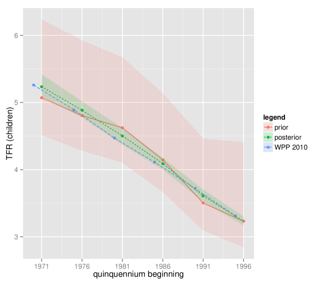
(a)

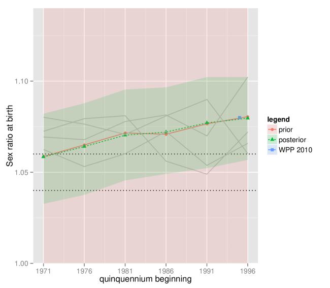
(b)

Figure 1: Prior and posterior medians and 95 percent credible intervals for the reconstructed population of India, 1971–2001: LABEL:sub@fig:indi-res-tfr total fertility rate (TFR); LABEL:sub@fig:indi-res-srb sex ratio at birth (SRB)(four trajectories from the Markov chain Monte Carlo (MCMC)sample are also shown).

Results for $e_{0}$ are shown in Figure 2. Life expectancy at birth increased for both sexes over the period of reconstruction (Figure 2a) but the sex difference suggests that female $e_{0}$ might have increased more rapidly than male $e_{0}$ and even exceeded it in the period 1996–2001 (Figure 2c). The mean interval half-width for the sex difference in life expectancies is 1.7 years. The posterior probabilities that female $e_{0}$ exceeded male $e_{0}$ support this (Table 1b). The possibility of an increase in the female$-$male difference in $e_{0}$ was investigated using the same method applied to SRB. The probability of an increase between 1971 and 2001 is 0.98 and the probability that the slope is greater than zero is 0.98 (Table 2b); strong evidence of a positive time trend.

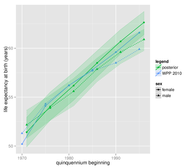
(a)

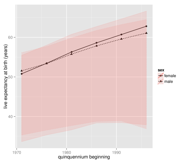
(b)

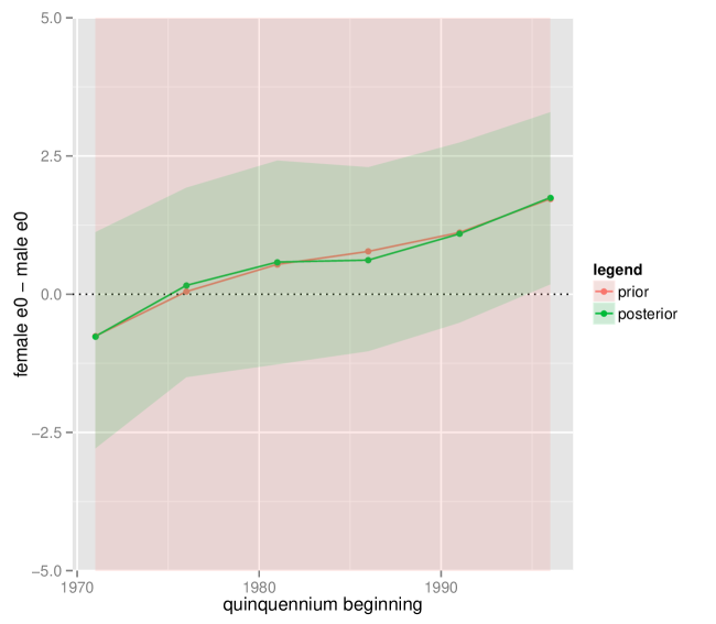
(c)

Figure 2: Prior and posterior medians and 95 percent credible intervals for life expectancy at birth ($e_{0}$)for the reconstructed population of India, 1971–2001. LABEL:sub@fig:indi-res-leb-femaleVSmale: Female and male posterior quantiles with World Population Prospects (WPP)2010 estimates; LABEL:sub@fig:indi-res-leb-femaleVSmale-prior: Female and male prior quantiles only; LABEL:sub@fig:indi-res-leb-female-male-difference: Sex difference (female$-$male).

Population sex ratios are shown in Figure 3a. The probability of a decrease in SRTP is 1 and the probability that the OLS slope was less than zero is 1 (Table 2c); very strong evidence for a decline over the period of reconstruction. Sex ratios in the population under five (SRU5s) increased in the WPP population counts, but our posterior median remained relatively constant after an initial decline. The probability that the sex ratio declined is 0.8;. the probability that the OLS coefficient was negative is 0.71 (Table 2d). Mean half-widths of the intervals for SRTP and the sex ratio in ages 0–5 are 0.01 and 0.027 respectively. Uncertainty is higher in years without a census.

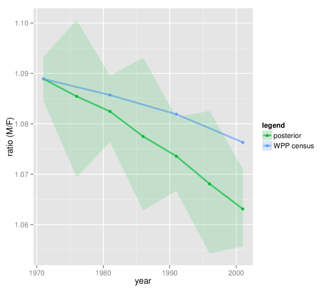
(a)

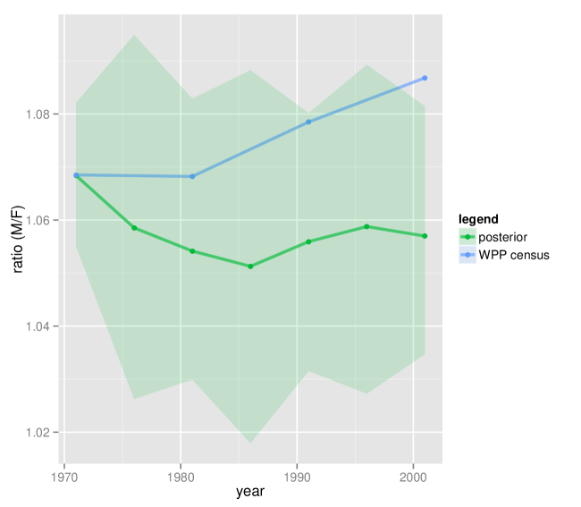
(b)

Figure 3: Prior and posterior medians and 95 percent credible intervals for sex ratios in the reconstructed population of India, 1971–2001. LABEL:sub@fig:indi-res-prtp: Total population; LABEL:sub@fig:indi-res-pr05: Population aged 0–5.

Table 1: Probability that sex ratios and differences exceeded certain thresholds for the reconstructed population of India, 1971–2001, by quinquennium.

1971	1976	1981	1986	1991	1996
(a) $\Pr(\text{{SRB}}>1.06)$
0.44	0.66	0.83	0.86	0.93	0.96
(b) $\Pr(\text{{female} $e_{0}$}-\text{{male} $e_{0}$}>0)$
0.21	0.58	0.74	0.78	0.91	0.99

Table 2: Probabilities of increasing linear trends for sex ratio at birth (SRB), sex difference in life expectancy at birth (sex diff. $e_{0}$), sex ratio in the total population (SRTP), and sex ratio in the population under five (SRU5)for the reconstructed population of India, 1971–2001. Two measures of trend are used: the difference over the period of reconstruction and the slope coefficient from the ordinary least squares (OLS)regression on the start year of each quinquennium. Ninety-five percent credible intervals for the measures are also given.

Measure of trend	95 percent CI	Prob $>$ 0
(a) Sex ratio at birth (SRB)
SRB 1996 $-$ SRB 1971	[$-$0.011, 0.054]	0.92
OLS slope (SRB $\sim$ year)	[$-$0.00034, 0.0021]	0.93
(b) Sex difference in life expectancy at birth (sex diff. $e_{0}$)
(sex diff. $e_{0}$)1996 $-$ (sex diff. $e_{0}$)1971	[0.12, 5]	0.98
OLS slope (sex diff. $e_{0}$ $\sim$ year)	[0.0066, 0.17]	0.98
(c) Sex ratio in the total population (SRTP)
SRTP 1996 $-$ SRTP 1971	[$-$0.034, $-$0.017]	0.000027
OLS slope (SRTP $\sim$ year)	[$-$0.0013, $-$0.00045]	0.00035
(d) Sex ratio in the population under five (SRU5)
SRU5 1996 $-$ SRU5 1971	[$-$0.037, 0.017]	0.2
OLS slope (SRU5 $\sim$ year)	[$-$0.0011, 0.00062]	0.29

Using the sex ratio, the probability that female U5MR exceeded that of males ranged from 0.72 to 0.89 over the period of reconstruction. Evidence of a linear trend was not found. Further results for U5MR and net international migration, are given in the appendices.

3.2.2 Thailand, 1960–2000

Total fertility rate fell very steeply in Thailand from 1960–2000 (Figure 4a). Posterior uncertainty about this parameter is small; the mean half-width of the posterior intervals is 0.07 children per woman.

Ninety five percent credible intervals for SRB contain the typical range of 1.04–1.06 for all but the first two quinquennia (Figure 4b). The probability that SRB exceeded 1.06 in each period is given in Table 3. There is strong evidence that SRBs were atypically high in the period 1960–1969. The time trend for SRB appears to be curvilinear, hence the simple linear summaries used to analyze the trend in Indian SRB are not appropriate here. Piecewise linear regression models are available [40, 41, e.g.,], but each trajectory in the posterior sample consists of only eight values and they are quite volatile. These characteristics make identification of a change point difficult. Instead we partition the period of reconstruction into two sub-periods, 1960–1984 and 1985–2000, and summarize the time trend with the following two difference quantities: $\text{SRB}_{1960}-\text{SRB}_{1980}$ and $\text{SRB}_{1985}-\text{SRB}_{1995}$ (the subscripts indicate the start years of the quinquennia). The posterior joint probability of a decrease from 1960 to 1984 followed by an increase to 1995–1999 (i.e., $\Pr(\{\text{SRB}_{1960}-\text{SRB}_{1980}>0\}\cap\{\text{SRB}_{1985}-\text{SRB}_{1995}<0\})$) is 0.84.

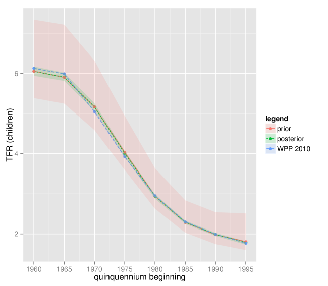
(a)

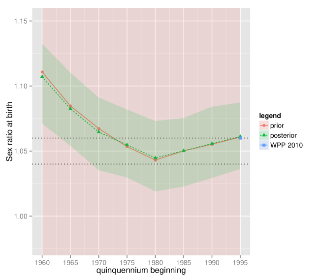
(b)

Figure 4: Prior and posterior medians and 95 percent credible intervals for the reconstructed population of Thailand, 1960–2000: LABEL:sub@fig:thai-res-tfr total fertility rate (TFR); LABEL:sub@fig:thai-res-srb sex ratio at birth (SRB).

Table 3: Probability that sex ratio at birth (SRB)was greater than 1.06 for the reconstructed population of Thailand, 1960–2000, by quinquennium.

1960	1965	1970	1975	1980	1985	1990	1995
0.99	0.95	0.66	0.32	0.11	0.19	0.35	0.54

Results for the sex difference in $e_{0}$ are shown in Figure 5. Our posterior intervals for the sex difference in $e_{0}$ lie entirely above zero in each quinquennium, suggesting that female longevity was greater than that of males in Thailand from 1960–2000 (mean half-width of the difference: 2.4 years). There is also strong evidence for a positive trend; the probability that the simple difference (1995 period minus 1960 period) in the sex differences in $e_{0}$ was greater than 0 is 0.96 and the probability that the OLS slope is greater than 0 is 1 (Table 4).

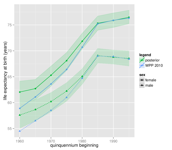
(a)

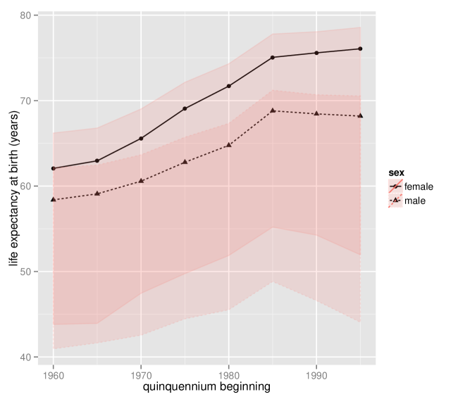
(b)

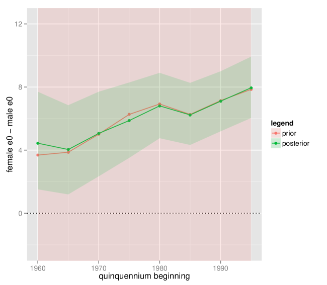
(c)

Figure 5: Prior and posterior medians and 95 percent credible intervals for life expectancy at birth ($e_{0}$)for the reconstructed population of Thailand, 1960–2000. LABEL:sub@fig:thai-res-leb-femaleVSmale: Female and male posterior quantiles with World Population Prospects (WPP)2010 estimates; LABEL:sub@fig:thai-res-leb-femaleVSmale-prior: Female and male prior quantiles only; LABEL:sub@fig:thai-res-leb-female-male-difference: Sex difference (female$-$male).

The posterior for sex ratio of under-five mortality rate (SRU5MR) suggests that mortality at ages 0–5 was similar for both sexes. In no quinquennium is there convincing evidence for a male-to-female ratio less than one. Similarly there is not strong evidence for a linear trend in this parameter over the period of reconstruction. Details are in the appendices along with results for net international migration and population sex ratios.

Table 4: Probabilities of an increasing linear trend and 95 percent credible intervals for sex difference in life expectancy at birth (sex diff. $e_{0}$)for the reconstructed population of Thailand, 1960–2000. Two measures of trend are used: the difference over the period of reconstruction and the slope coefficient from the ordinary least squares (OLS)regression on the start year of each quinquennium.

Measure of trend	95 percent CI	Prob $>$ 0
(sex diff. $e_{0}$)1996 $-$ (sex diff. $e_{0}$)1971	[$-$0.42, 7.1]	0.96
OLS slope (sex diff. $e_{0}$ $\sim$ year)	[0.027, 0.18]	1

3.2.3 Laos, 1985–2004

Medians and prior and posterior credible intervals for TFR and SRB are shown in Figure 6. The posterior for TFR obtained here (Figure 6a) is very similar that obtained by [96] who reconstructed the female-only population and did not estimate SRB; it was kept fixed at 1.05 throughout, a demographic convention [70].

There was very little data on SRB for Laos therefore, in this study, the initial estimate of SRB was fixed at 1.05 in all quinquennia but a posterior distribution was estimated using the model. The posterior median SRB deviates very little from the initial estimate, although the uncertainty has been considerably reduced; the mean of the half-widths of the 95 percent credible intervals is 0.038 compared with 0.39 for the prior (Figure 6b). The probability that SRB was above 1.06 in any of the quinquennia is low (Table 5) and the evidence for a trend over time is equivocal (Table 6).

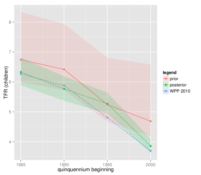
(a)

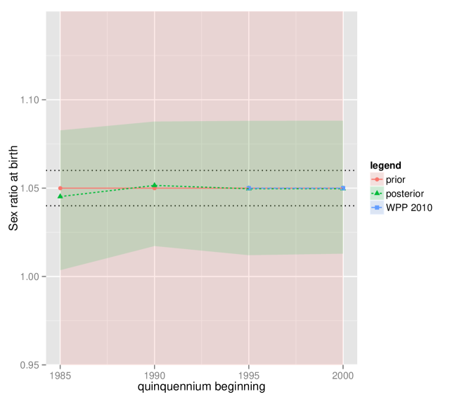
(b)

Figure 6: Prior and posterior medians and 95 percent credible intervals for the reconstructed population of Laos, 1985–2004: LABEL:sub@fig:laos-res-tfr total fertility rate (TFR); LABEL:sub@fig:laos-res-srb sex ratio at birth (SRB).

There is strong evidence that female $e_{0}$ was higher from 1990 through 2005 but there appears to be no evidence for a sex difference between 1985 and 1990 (Figure 7, Table 5b). The posterior distributions of both trend summaries provide strong evidence for an increase in the sex difference over the period of reconstruction (Table 6), although this is due primarily to the increase immediately following the 1985–1990 period.

Results for SRU5MR, net international migration and population sex ratios are in the appendices.

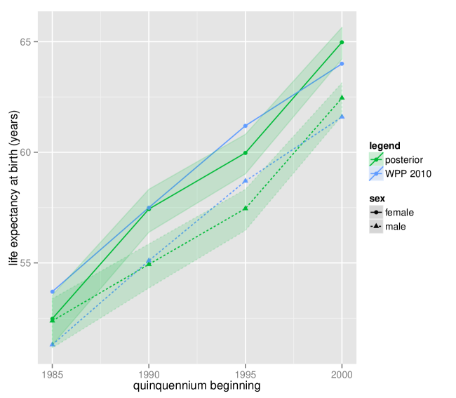
(a)

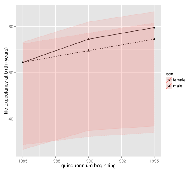
(b)

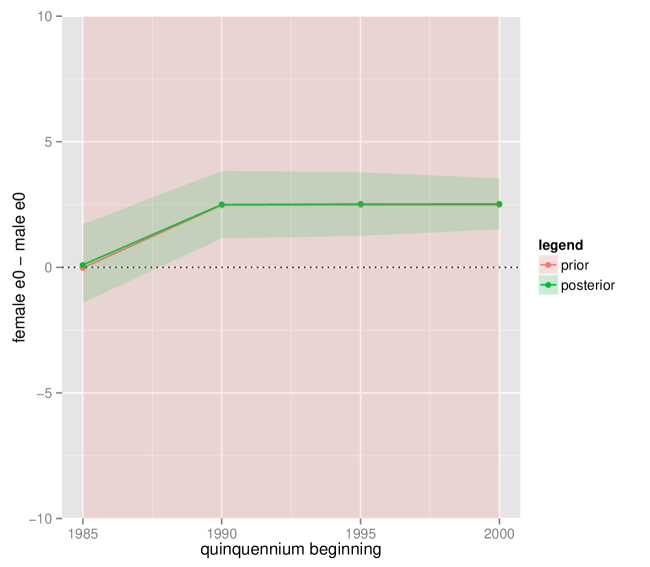
(c)

Figure 7: Prior and posterior medians and 95 percent credible intervals for life expectancy at birth ($e_{0}$)for the reconstructed population of Laos, 1985–2004. LABEL:sub@fig:laos-res-leb-femaleVSmale: Female and male posterior quantiles with World Population Prospects (WPP)2010 estimates; LABEL:sub@fig:laos-res-leb-femaleVSmale-prior: Female and male prior quantiles only; LABEL:sub@fig:laos-res-leb-female-male-difference: Sex difference (female$-$male).

Table 5: Probability that sex ratios and differences exceeded certain thresholds for the reconstructed population of Loas, 1985–2005, by quinquennium.

1985	1990	1995	2005
(a) $\Pr(\text{{SRB}}>1.06)$
0.20	0.30	0.27	0.27
(b) $\Pr(\text{{female} $e_{0}$}-\text{{male} $e_{0}$}>0)$
0.56	1.00	1.00	1.00

Table 6: Probabilities of an increasing linear trend and 95 percent credible intervals for sex difference in life expectancy at birth (sex diff. $e_{0}$)for the reconstructed population of Laos, 1985–2000. Two measures of trend are used: the difference over the period of reconstruction and the slope coefficient from the ordinary least squares (OLS)regression on the start year of each quinquennium.

Measure of trend	95 percent CI	Prob $>$ 0
(a) Sex ratio at birth (SRB)
SRB 2000 $-$ SRB 1985	[$-$0.046, 0.061]	0.58
OLS slope (SRB $\sim$ year)	[$-$0.0034, 0.0042]	0.56
(b) Sex difference in life expectancy at birth (sex diff. $e_{0}$)
(sex diff. $e_{0}$)2000 $-$ (sex diff. $e_{0}$)1985	[0.54, 4.2]	0.99
OLS slope (sex diff. $e_{0}$ $\sim$ year)	[0.025, 0.26]	0.99

4 Discussion

We have described Bayesian reconstruction for two-sex populations, a method of reconstructing human populations of the recent past which yields probabilistic estimates of uncertainty [97, 96]. We reconstructed the populations of Laos from 1985–2005, Thailand from 1960–2000 and India from 1971–2001, paying particular attention to sex ratios of fertility and mortality indicators. We estimate that the posterior probability that SRB was above 1.06 is greater than 0.9 in India between 1991 and 2001 and the probability it increased over this period is about 0.92. The SRB was also above 1.06 with high posterior probability in Thailand from 1960–1970. We estimate that the probability it decreased between 1960 and 1980, then increased from 1985 to 2000, is 0.84. We found no evidence for atypically high SRBs, or a trend over the period of reconstruction, for Laos, a country with much less available data than Thailand and India. In both Thailand and Laos, we found strong evidence that $e_{0}$ was greater for females and, in Thailand, that the difference increased over the period of reconstruction. In India, the probability that female $e_{0}$ was lower during 1971–1976 was 0.79 but there was strong evidence for a narrowing of the gap through to 2001.

In its original formulation, Bayesian reconstruction was for female-only populations; here we show how two-sex populations can be reconstructed using the same framework. The method takes a set of data-derived, bias-reduced initial estimates of age-specific fertility rates, and age-sex-specific survival proportions, migration proportions and population counts from censuses, together with expert opinion on the measurement error informed by data if available. Bayesian reconstruction updates initial estimates using adjusted census counts via a Bayesian hierarchical model. The periods of reconstruction used in our applications begin in the earliest census year for which non-census vital rate data were available, and end with the year of the most recent census. Reconstruction can be done further ahead, but without a census the results are based purely on the initial estimates.

The initial estimates, $f_{a,t}^{*}$, $s_{a,t,l}^{*}$, $g_{a,t,l}^{*}$, $n_{a,t_{0},l}^{*}$, $\text{{\footnotesize{SRB}}}_{t}^{*}$, enter the model as fixed prior medians (Section 2.3), and so the posterior will be sensitive to changes in these inputs. This is actually desirable, because the initial estimates are based heavily on data specific to that estimate; the posterior should be sensitive to changes in these data.

Information about measurement error variance is needed to set the model hyper parameters (14). In our case studies, this took the form of expert opinion, elicited as 90percent probability intervals centred at the data-derived initial estimates. If available, additional data on measurement error could be used to inform the elicitations, or to replace them altogether if they are comprehensive enough. This is the case in many developed countries (e.g., New Zealand, [96]), where post-census enumeration surveys and vital registration coverage studies are undertaken. However, we expect Bayesian reconstruction to be most useful for less developed and developing countries where fragmentary and unreliable data lead to a substantial amount of uncertainty. For these countries, expert opinion is a main source of information. We do expect the posterior to be somewhat sensitive to the elicited intervals since the initial estimates themselves do not contain much information about measurement error.

Previous methods of population reconstruction were purely deterministic, were not designed to work with the type of data commonly available for many countries over the last sixty years, or did not account for measurement error [53, 54, 99, 8, e.g.,]. [22] used a Bayesian approach to construct a counterfactual population, but age patterns of fertility were held fixed and mortality varied only through infant mortality. Bayesian reconstruction does not impose fixed age-patterns and mortality can vary at each age. Moreover, international migration is estimated in the same way as fertility and mortality.

We considered sex ratios of births and mortality because these are of interest to demographers and policy-makers, especially since they determine the SRTP [29, 30]. It is conventional to compare sex-specific U5MRs with a ratio but sex-specific $e_{0}$s with a difference. We have not studied the associations among U5MR ratios, $e_{0}$ differences and population sex ratios. The SRTP is a function of life-time cohort mortality but the U5MR and $e_{0}$ presented here are period measures for which the relationship used by [30] does not hold. Our results add to previous work on SRMs, especially that of [73] who studied sex ratios of U5MR and called for further work to quantify its uncertainty. [73] decomposed U5MR into mortality between ages 0 and 1 (infant mortality) and mortality between ages 1 and 5 (child mortality). We reconstructed populations in age- time-intervals of width five because these are the intervals for which data is most widely available across all countries.

Many methods of adjusting vital registration using census data have been proposed [7, 37, 57, e.g.,], but these deal with intercensal migrations by essentially truncating the age groups most affected by migration [63], or ignore them altogether. [58] and [38] applied these methods to Thailand to estimate undercounts. The aim of these methods is to produce improved point estimates of vital rates. We have not used any census data to derive our initial estimates. For example, initial estimates of survival were not based on inter-censal cohort survival and initial estimates of migration were not based on “residual” counts. Doing so would have amounted to using the census data twice and would have underestimated the uncertainty. The outputs of Bayesian reconstruction are interval estimates which quantify uncertainty probabilistically.

4.1 Sex Ratios in Asia

The SRTP is a crude measure of the balance of sexes in a population since it is not age-specific; sex ratios may be quite different among age groups, for example. Nevertheless, there is a large literature devoted to estimating SRTPs and exploring the causes and consequences, especially in Asia where SRTPs are the highest in the world [87]. A persistently high sex ratio among younger cohorts could lead to a “marriage squeeze” in which many young males will struggle to marry due to a lack of eligible females [35]. Formally, high SRTPs are the result of high SRBs and life-time sex ratios of cohort mortality [30]. The relative effects of these two factors may vary by time and country.

A normal range for SRB is believed to be 1.04–1.06 [88]; on average, slightly more than half of all newborns are male. Concerns about quality, or a complete lack of data, have made it difficult to accurately estimate SRBs in many Asian countries. Bayesian reconstruction of these populations quantifies the accuracy of SRB estimates probabilistically.

With very few exceptions, country-level $e_{0}$s for females exceed those of males. This pattern is consistent with a female survival advantage; in virtually all contemporary human populations, females age slower and live longer than males [76, 90]. Behavioural factors appear to play an important role, especially in developed countries where the prevalence of harmful activities, such as smoking, consumption of alcohol, and risky behaviour leading to accidental death, tends to be lower among women than among men [93, 94, 51]. The persistence of lower male $e_{0}$ across the development spectrum suggests there are other factors as well. In less developed countries, $e_{0}$ is determined more by infant and child mortality. [68] studied infant mortality in Africa and found an association with parental characteristics extant prior to conception. Biological, as well as behavioural, determinants have also been proposed but there is little consensus on the specific mechanism [4]. The only countries in which female $e_{0}$ is not higher are countries in Africa and some in South and Central Asia. The African countries are those with generalized HIV epidemics where mortality due to AIDS changes the typical sex difference in $e_{0}$ [87]. Those in Asia include, most notably, India where cultural preference for males is thought to be the major cause.

4.1.1 India

The SRTP in India has received considerable attention, particularly as an indicator of discrimination against women [88]. [29] showed that only slightly elevated SRBs and SRMs at young ages are sufficient to produce the observed SRTP in India, if they persist for a long period of time. The relative contribution of these two factors may have varied over time. [11] and [31, 34] argue that India experienced a transition in the 1970s whereby high SRB replaced low SRM as the cause of the high SRTPs observed throughout the period (recall that a low SRM is a result of lower male mortality). Evidence suggests that low SRMs were due to female neglect and infanticide. In the 1970s, these practices gave way to sex selective abortion which raised the SRB instead.

The transition hypothesis is based on several pieces of evidence. Data suggest a possible rise in SRB in India above the typical range of 1.04–1.06 in the mid 1980s [31]. In the 1970s, amniocentesis started to became available as a method for determining the sex of a foetus and abortion was legalized. Ultrasonography, a less invasive way of determining foetal sex, started to became available in many parts of India in the 1980s. In certain regions, such as the northern states and highly urbanized areas, there is a long standing tradition of preference for sons over daughters [60, 12]. The arrival of these new technologies in this context appears to have led to an increase in sex selective abortions in India [11, 32, 42, 88, 44]. The steep decline in Indian TFR, which began in the early 1970s, could have increased the prevalence of such procedures. Several studies have found evidence that SRB is higher at higher parities (birth orders), both in India [24, 11, 43, 44] and other Asian countries [23]. The increase appears to be greater if none of the earlier births were male. As TFR decreases so does the average family size, so the risk of having no sons increases [34]. Therefore, in cultures where sons play important economic and social functions, or where families benefit materially much more from the marriage of a son than of a daughter, the incentive to use sex selective abortion increases [60, 34].

After combining all available data and including uncertainty, we estimate that the probability there was an increase in SRB between 1971 and 2001 is above 0.92. The probability that female U5MR was higher over this period is estimated to be between 0.72 and 0.89, but there was no evidence of a trend. Therefore, our results provide support for the SRB part of the transition hypothesis but not the U5MR part.

Overall mortality decreased rapidly in India from about 1950 as infectious diseases were brought under control, food security increased and health services became more widely available [11]. Our results suggest that, after taking account of uncertainty, there was an increase in $e_{0}$ and a continual decrease in U5MR between 1971 and 2001 for both sexes. Using Sample Registration System data, [11] noted that the decrease was greater for females than males and our analysis of the change in the sex difference of $e_{0}$ supports this; we found that the probability that the difference increased over the period of reconstruction is about 0.98. The probability of a decline in the SRTP was found to be similarly strong. However, as with SRU5MR, there was little evidence for a trend in SRU5.

India’s large population makes it a very important case for the study of sex ratios in Asia [31] and, like other authors [30, 87, e.g.,], we have focused on country level estimates only. However, where available, data suggest that there are large regional variations in SRBs and population sex ratios, with estimates for urban areas and northern states being much higher than other areas [11, 34, 44]. Currently, Bayesian reconstruction is not able to produce sub-national estimates, but could be extended to do so in the future.

4.1.2 Thailand

Like other parts of Asia, Thailand experienced rapid economic growth and a rapid fall in TFR beginning in 1960. The TFR decline was accompanied by an increase in the widespread use of modern contraceptive methods made available through government supported, voluntary family planning programs [45, 47, 50]. Unlike India, Thailand is not considered to have had a high SRB [34]. Vital registration data, which formed the basis of our initial estimates, indicate that SRB was high during the period 1960 to 1970, but remained within the typical range thereafter. This is consistent with studies conducted after the early 1970s which found that small families of two or three children consisting of at least one boy and one girl was the most commonly desired configuration in Thailand. TFR decline in Thailand may have intensified this preference [49, 50].

Posterior intervals for sex ratios of mortality in Thailand reflect the typical pattern which is one of higher female life expectancy. There is no evidence that this pattern was also true for U5MR (on-line resources).

4.1.3 Laos

Fertility in Laos remained high relative to its neighbours. For example, the estimated TFR for 1985 in Laos is comparable to the 1960 estimate for Thailand [26]. Posterior uncertainty about SRB is high and our results provide no evidence to suggest levels were atypical between 1985 and 2005. All-age mortality as summarized by $e_{0}$ does appear to have been higher for females from 1990 onward but, as with Thailand, there is no evidence that this advantage held for U5MR (on-line resources).

4.2 Further Work and Extensions

Our prior distributions were constructed from initial point estimates of the CCMPP input parameters, together with information about measurement error. In the examples given here, this was elicited from UN analysts who are very familiar with the data sources and the demography of each country. In cases where good data on measurement error are available, they can be used. For example, [96] used information from post-enumeration surveys to estimate the accuracy of New Zealand censuses. Data of this kind are rarely available in developing countries for either census or vital rate data. Nevertheless, surveys come with a substantial amount of meta-data which can be used to model accuracy. This approach was taken by [2] who developed a method for estimating the quality of survey-based TFR estimates in West Africa by modelling bias and measurement error variance as a function of data quality covariates. [97] used these results in their reconstruction of the female population of Burkina Faso. Extending this work to more countries could provide a source of initial estimates together with uncertainty that could be used as inputs to Bayesian reconstruction.

Posterior uncertainty in estimates of U5MR was found to be substantial and we did not find strong evidence for a skewed sex ratio in any of our examples. U5MR is under-identified in the model because the only census count it affects, that for ages 0–5, is also dependent on SRB and TFR. Recent work by the UN Interagency Group for Child Mortality Estimation (IGME) has focused on producing probabilistic estimates of U5MR [39, 1]. Further work could look at ways of using these estimates in Bayesian reconstruction to improve estimation of U5MR.

The census counts we used were not raw census output but adjusted counts published in WPP. In some cases, these counts are adjusted by the UNPD to reduce bias due to factors such differential undercount by age. This may have led to an underestimate of uncertainty. The use of raw census outputs instead is worth investigating, but the effects of undercount would still need to be addressed through modifications to the method.

Our prior distributions for international migration were centred at zero with large variances. This is a sensible default when accurate data are not available. Further work could investigate the possibility of using stocks of foreign-born, often collected in censuses, to provide more accurate initial estimates. Data on refugee movements is another source that could be investigated where available.

We have reconstructed national level populations only, principally because this is the level at which the UN operate. We have already mentioned that sub-national reconstructions might be of interest. Subnational reconstructions could be done without any modifications to the method if the requisite data are available; national level initial estimates and population counts would just be replaced with their subnational equivalents and the method applied as above. Reconstructing adjacent regions, or regions between which there is likely to be a lot of migration would require special care, however, as there is no way of accounting for dependence among migratory flows under the current approach.

Appendix A Derivation of Demographic Indicators

A.1 Total Fertility Rate

The TFR for the period $[t,t+5)$ is the average number of children born to women of a hypothetical cohort which survives through ages $a_{L}^{\text{[fert]}}$ to $a_{U}^{\text{[fert]}}$, all the way experiencing the age-specific fertility rates, $f_{a,t}$. Its definition is:

$$\mathit{TFR}_{t}\equiv 5\cdot\sum_{a_{L}^{\text{[fert]}}}^{a_{U}^{\text{[fert]}}}f_{a,t}.$$

A.2 Life Expectancy at Birth

Life expectancy at birth is the average age at death for members of a hypothetical cohort which, at each age, experience age-specific survival $s_{a,t,l}$. Its definition is:

$$e_{0,t,l}=5\sum_{a=0}^{A}\prod_{i=0}^{a}s_{i,t,l}+5\left(\prod_{i=0}^{A}s_{i,t,l}\right)\bigl{(}s_{A+5,t,l}/(1-s_{A+5,t,l})\bigr{)}.$$

The derivation is straightforward and can be found in [97].

A.3 Under 5 Mortality Rate

The U5MR is constructed in the same way as the standard “Infant Mortality Rate” [70, e.g.,], except for the age interval [0,5). It is defined as follows:

$$\mathit{U5MR}_{t}\equiv\frac{\text{No.\ deaths to those aged [0,5) in the interval [$t$,$t$+5)}}{\text{No.\ births in the interval [$t$,$t$+5)}}.$$

It is neither a true demographic rate nor a probability but, nevertheless, is in common use.

Appendix B Application: Further Details About Data Sources

B.1 India

B.1.1 Population Counts

Censuses were conducted in 1971, 1981, 1991 and 2001. We used the counts in WPP 2010 which were adjusted for slight undercount in some age groups.

B.1.2 Sex Ratio at Birth

Data on sex ratio at birth came from the same sources as data on age-specific fertility (Section B.1.3). A weighted cubic spline was used to smooth the available data and initial estimates were derived by evaluating the spline at the mid-points of the quinquennia 1971–1976, …, 1996–2001. Elicited relative error for this parameter was set at 10 percent.

B.1.3 Fertility

Initial estimates of age-specific fertility were based on data from the Indian Sample Registration System (SRS) [83] and National Family Health Surveys (NFHSs) conducted between 1992 and 2006 [82]. These were weighted and smoothed using the same procedure as for Thailand. Elicited relative error for this parameter was set at 10 percent.

B.1.4 Mortality

Initial estimates of survival proportions were calculated from abridged life tables based on data from the SRS from 1968-1969 through 2008. The average number of person-years lived in each interval (${}_{n}a_{x}$s) were computed using [28]’s Greville_Short_TRotAIoA_1943 formula from age 15 and above. Values for ages under 5 are based on the formulae of [20] using the West pattern. All other values were set to 2.5 [84, see also].

Additional sources were used for infant and child mortality: data on births and deaths under-five were calculated from maternity-history data from the NFHSs conducted between 1992 and 2006 and data on children ever-born and surviving classified by age of mother from these surveys and earlier ones as well as from the 2002–04 Reproductive and Child Health Survey (RCHS). Weighted cubic splines were used to smooth estimates of ${}_{1}q_{0}$ and ${}_{4}q_{1}$ from these data sources. The weights were determined by UN analysts based on their expert judgement about the relative reliability of each source. Elicited relative error was set to 10 percent.

B.1.5 Migration

We used the same initial estimates for international migration as for Laos.

B.2 Thailand

B.2.1 Fertility

Initial estimates of age-specific fertility were based on direct and indirect estimates of current fertility and CEB taken from the Surveys of Population Change conducted between 1964 and 1996 [78, 79, 80, 81]; see also [89], the World Fertility Surveys (WFSs) [86], the Thai Longitudinal Study of Economic, Social and Demographic Change [48], the 1968–1972 Longitudinal Study of Economic, Social and Demographic Change [64], the 1978 and 1996 National Contraceptive Prevalence Surveys [77, 18], the 1987 Demographic and Health Survey (DHS), and vital registration.

Age patterns and levels of fertility were estimated separately from the available data. The available data were smoothed within age and within year using weighted splines. The weights were determined by UN analysts based on their expert judgement about the relative reliability of each source. Estimates of TFR, based on summed age-specific estimates, were obtained similarly. The final set of initial estimates was obtained by multiplying the smoothed TFRs by the smoothed age patterns. Elicited relative error for this parameter was set at 10 percent.

B.2.2 Mortality

Initial estimates of mortality for both sexes were based on life tables calculated from vital registration. Vital registration is thought to have underestimated U5MR [38] so the following additional sources were used to derive initial estimates of under five mortality: (a) the 1974–1976, 1984–86, 1989, 1991, 1995–1996, Surveys of Population Change [78, 79, 80, 81], (b) maternity-history data from the 1975 WFS and 1987 DHS, (c) data on children ever born and surviving from these surveys, the 1981–1986 Contraceptive Prevalence Surveys (CPSs). All available non-census data on ${}_{5}q_{0}$ from these sources were weighted by UN analysts who used their expert judgement about potential biases and smoothed over time using cubic splines. The splines were evaluated at 1962.5, 1968.5, …1998.5 and the values substituted for the ${}_{5}q_{0}$s in the life tables based solely on vital registration. Survival proportions were derived from these “spliced” life tables.

B.3 Laos

Initial estimates for females were the same as those used by [96]. Initial estimates for males were derived using the same procedures.

B.3.1 Population Counts

National censuses were conducted in 1985, 1995 and 2005. Following [96], we used the census year counts in WPP 2010; there were no post-enumeration surveys, but these counts were adjusted to compensate for undercount in certain age groups.

B.3.2 Fertility

Direct and indirect estimates were based on CEB and recent births (preceding 12 and 24 months), all by age of mother, collected by the 1993 Laos Social Indicator Survey, the 1995 and 2005 censuses, the 1994 Fertility and Birth Spacing Survey, the 2000 and 2005 Lao Reproductive Health Surveys, the 1986–1988 multi-round survey and the 2006 MICS3 survey. [100]’s Zaba_Use__1981 Relational Gompertz Model, [3]’s Arriaga_Estimating_1983 method, the $P/F$ method [14], [3]’s Arriaga_Estimating_1983 modified $P/F$ method and the Brass fertility polynomial [15, 17] were used to derive indirect estimates.

Age patterns of fertility were estimated by taking medians across all available data points within the quinquennia 1985–1990, …, 2000–2005. TFR was estimated separately by converting each age-specific data series into series of TFR by summing. Medians within quinquennia were then taken. The final initial estimates of the age-specific rates was obtained by multiplying the median age-patterns by the median TFRs. Data points were not weighted.

The elicited relative error was set to 10 percent. Hence, the medians of the initial estimate distributions for age-specific fertility rates were the initial point estimates and the upper 95 percent and lower five percent quantiles were equal to the initial point estimates plus and minus 10 percent, respectively.

B.3.3 Mortality

The available data only provide estimates of mortality under age five. These are maternity histories and CEB and surviving data from the 1993 Laos Social Indicator Survey, the 1994 Fertility and Birth Spacing Survey, the 1995 and 2000 censuses and the 2000 and 2005 Lao Reproductive Health Surveys (intercensal survival estimates were not used). Weighted cubic smoothing splines were used to smooth these to produce single initial point estimates of the average ${{}_{1}}{q}_{0}$ and ${{}_{5}}{q}_{0}$ over each quinquennium 1985–1990, …, 2000–2005. For each quinquennium, two Coale and Demeny West (CD West) life tables were found; one with ${{}_{1}}{q}_{0}$ closest to that produced by the smoothing procedure and one with ${{}_{5}}{q}_{0}$ closest. Within each pair, the $e_{0}$s in these two tables were averaged. Age-specific survival proportions calculated from the CD West table with $e_{0}$ closest to this average were then taken as the initial estimates of mortality at all ages. The elicited relative error of these initial point estimates was set to 10 percent.

B.3.4 Migration

There is very little quantitative information about international migration in Laos between 1985 and 2005. To reflect this, initial estimates for females and males were set to zero and the elicited relative error was high, at 20 percent.

Appendix C Application: Further Results

C.1 India

Results for U5MR are in Figure 8. Posterior medians of Indian U5MR for males are lower than those for females. However, although the sex ratio in U5MR is centred below one, the posterior intervals are relatively wide and contain it (mean half-width 0.16 deaths per live births; Figure 8). The probability that female U5MR exceeded that of males in each quinquennium is given in Table 7; by the period 1996–2001 this had peaked at 0.89. The evidence for a linear decrease over the period of reconstruction is weak (Table 8a). There is a slight decline in the posterior median after 1981 but the evidence for a trend after this point is similar: the probability of a simple decrease is 0.7 and the probability that the OLS coefficient was less than zero is 0.68 (Table 8b).

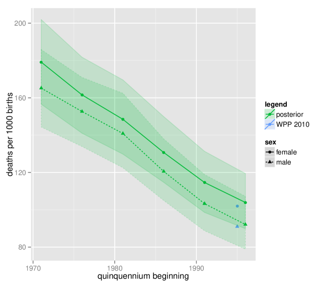
(a)

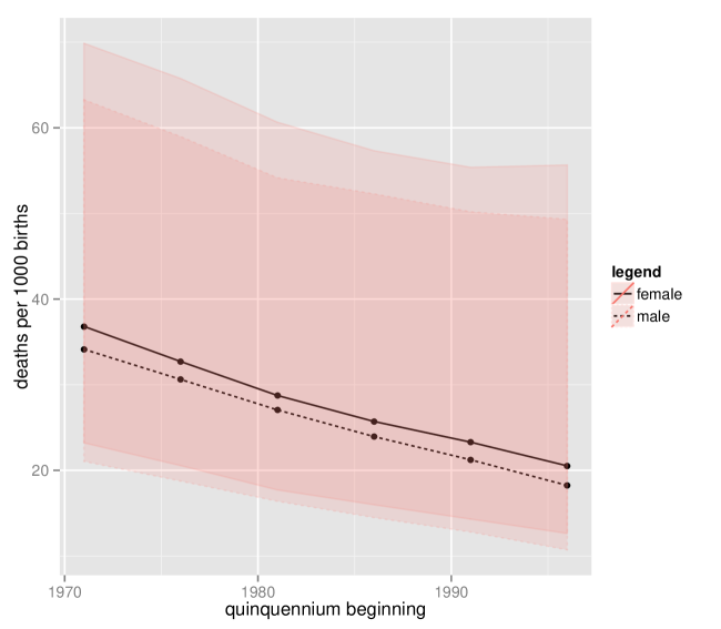
(b)

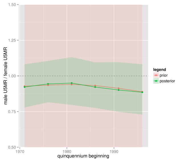
(c)

Figure 8: Prior and posterior medians and 95 percent credible intervals for under-five mortality rate (U5MR)(deaths per 1,000 live births) for the reconstructed population of India, 1971–2001 LABEL:sub@fig:indi-res-IMR-femaleVSmale: Female and male posterior quantiles and World Population Prospects (WPP)2010 estimates; LABEL:sub@fig:indi-res-IMR-femaleVSmale-prior: Female and male prior quantiles only; LABEL:sub@fig:indi-res-IMR-female-male-ratio: Male-to-female ratio.

Table 7: Probability that sex ratio of under-five mortality rate (SRU5MR)was less than one for the reconstructed population of India, 1971–2001, by quinquennium.

1971	1976	1981	1986	1991	1996
0.85	0.77	0.72	0.83	0.86	0.89

Table 8: Probabilities of an increasing linear trend and 95 percent credible intervals for sex ratio of under-five mortality rate (SRU5MR)for the reconstructed population of India, 1971–2001. Two measures of trend are used: the difference over the period of reconstruction and the slope coefficient from the ordinary least squares (OLS)regression on the start year of each quinquennium.

Measure of trend	95 percent CI	Prob $>$ 0
(a) Sex ratio of under-five mortality rate (SRU5MR), 1971–2001
SRU5MR 1996 $-$ SRU5MR 1971	[$-$0.26, 0.2]	0.38
OLS slope (SRU5MR $\sim$ year)	[$-$0.0097, 0.0061]	0.32
(b) Sex ratio of under-five mortality rate (SRU5MR), 1981–2001
SRU5MR 1996 $-$ SRU5MR 1971	[$-$0.3, 0.17]	0.3
OLS slope (SRU5MR $\sim$ year)	[$-$0.0097, 0.0061]	0.32

Results for the average annual net number of migrants are in Figure 9. The mean posterior half-width is 801,000.

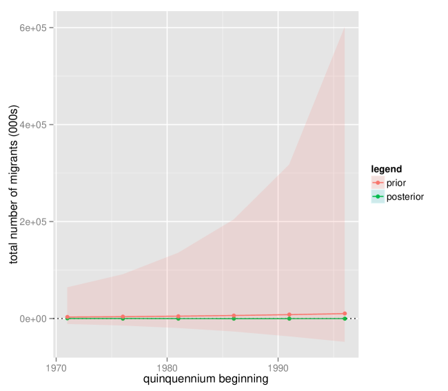
(a)

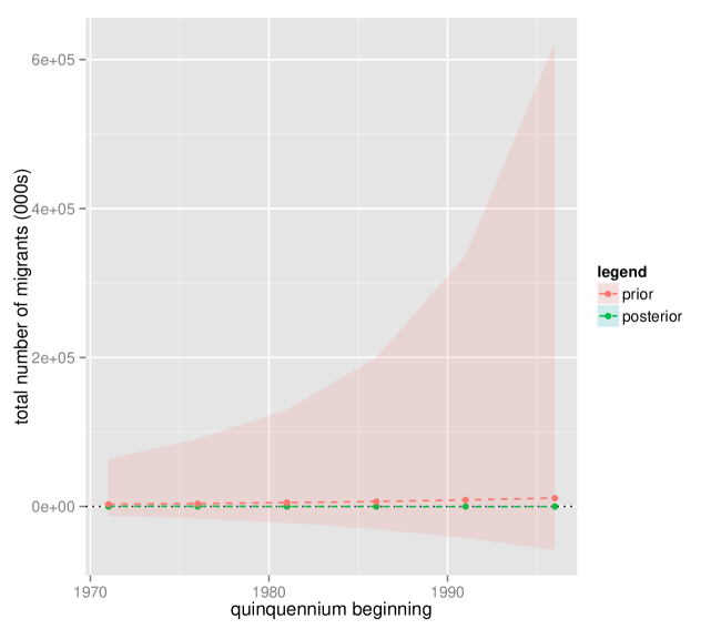
(b)

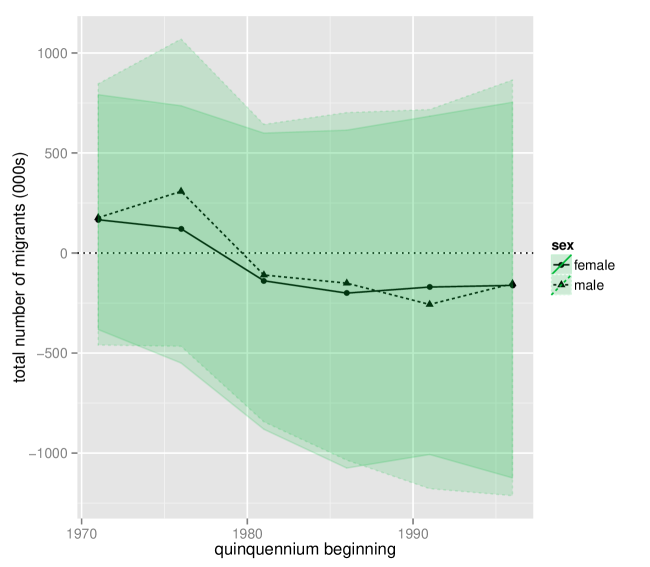
(c)

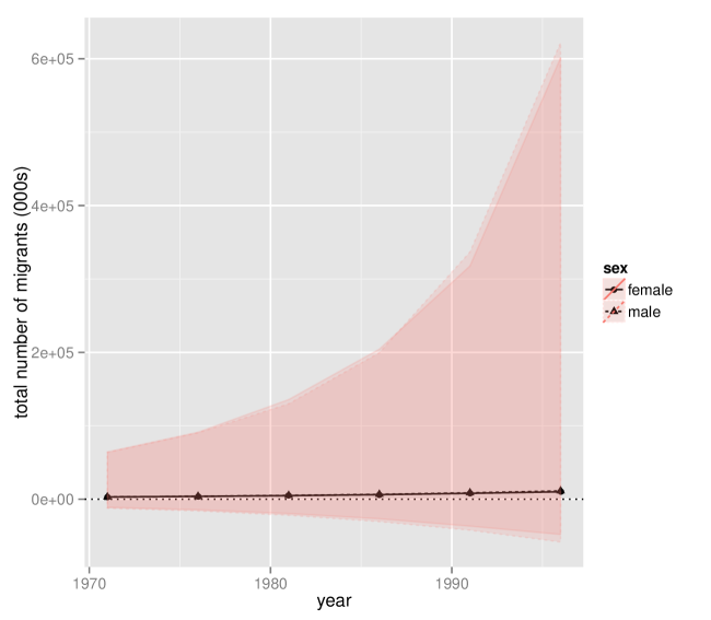
(d)

Figure 9: Prior and posterior medians and 95 percent credible intervals for the average annual net number of migrants for the reconstructed population of India, 1985–2004. LABEL:sub@fig:indi-res-totmig-female: Females; LABEL:sub@fig:indi-res-totmig-male: Males; LABEL:sub@fig:indi-res-totmig-femaleVSmale: Female and male posterior quantiles only; LABEL:sub@fig:indi-res-totmig-femaleVSmale-prior: Female and male prior quantiles only.

C.2 Thailand

Results for SRU5MR are shown in Figure 10. The posterior suggests mortality at ages 0–5 was similar for both sexes. The 95 percent credible interval is centred above one for the period of reconstruction (mean half-width 0.47) and the probabilities that the male-to-female ratios of U5MR were less than one are small (Table 9). Based on the measures of change over time used above, there is no evidence for a strong trend in this parameter over the period of reconstruction (Table 10).

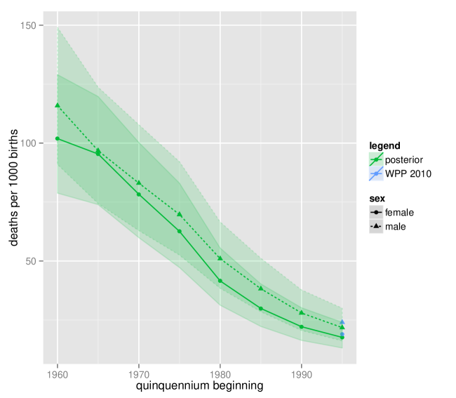
(a)

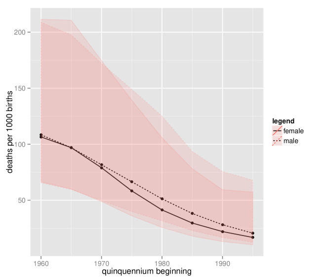
(b)

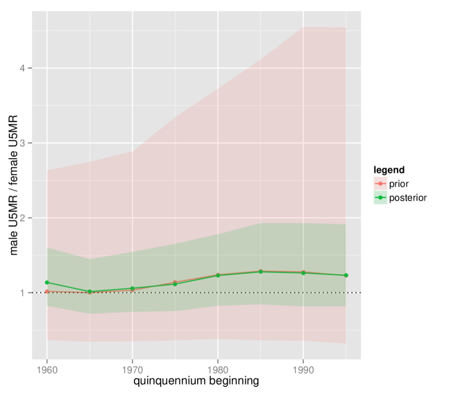
(c)

Figure 10: Prior and posterior medians and 95 percent credible intervals for under-five mortality rate (U5MR)(deaths per 1,000 live births) for the reconstructed population of Thailand, 1960–2000 LABEL:sub@fig:thai-res-IMR-femaleVSmale: Female and male posterior quantiles and World Population Prospects (WPP)2010 estimates; LABEL:sub@fig:thai-res-IMR-femaleVSmale-prior: Female and male prior quantiles only; LABEL:sub@fig:thai-res-IMR-female-male-ratio: Male-to-female ratio.

Table 9: Probability that sex ratio of under-five mortality rate (SRU5MR)was less than one for the reconstructed population of Thailand, 1971–2001, by quinquennium.

1960	1965	1970	1975	1980	1985	1990	1995
0.23	0.46	0.38	0.29	0.15	0.12	0.13	0.16

Table 10: Probabilities of an increasing linear trend and 95 percent credible intervals for sex ratio of under-five mortality rate (SRU5MR)for the reconstructed population of Thailand, 1960–2000. Two measures of trend are used: the difference over the period of reconstruction and the slope coefficient from the ordinary least squares (OLS)regression on the start year of each quinquennium.

Measure of trend	95 percent CI	Prob $>$ 0
SRU5MR 1996 $-$ SRU5MR 1971	[$-$0.54, 0.84]	0.61
OLS slope (SRU5MR $\sim$ year)	[$-$0.0075, 0.022]	0.81

Results for the average annual net number of migrants are in Figure 11. The mean posterior half-width is 85,800.

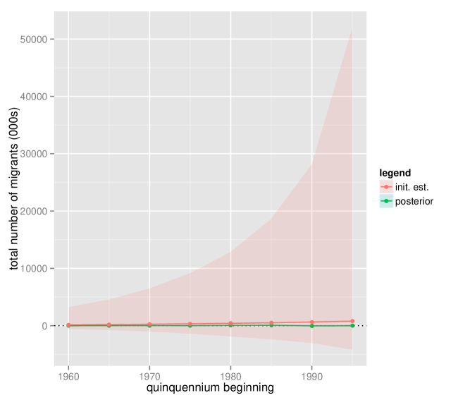
(a)

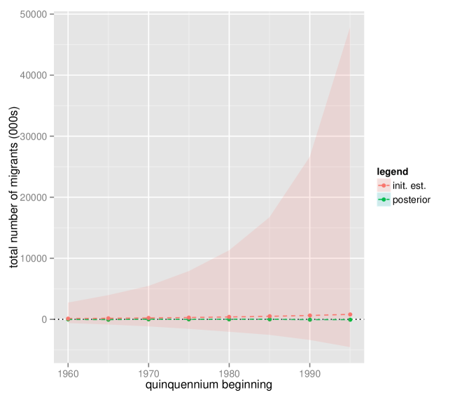
(b)

(c)

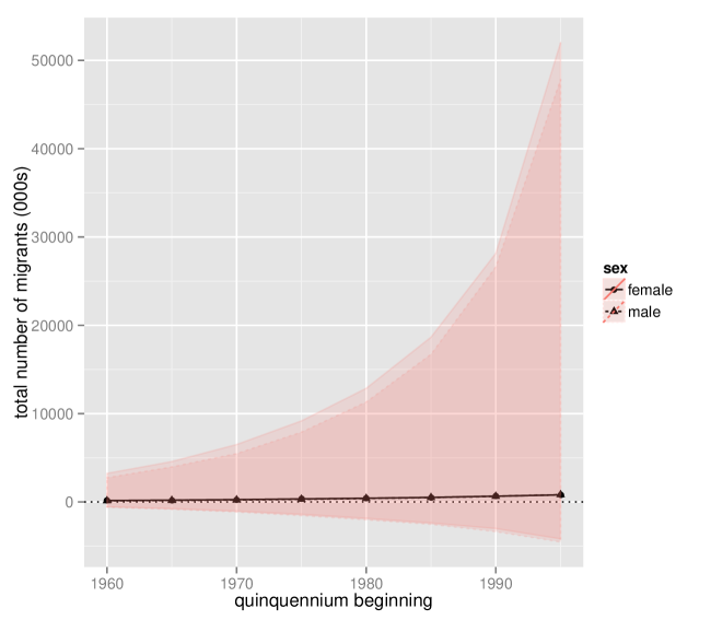
(d)

Figure 11: Prior and posterior medians and 95 percent credible intervals for the average annual net number of migrants for the reconstructed population of Thailand, 1985–2004. LABEL:sub@fig:thaiF2-res-totmig-female: Females; LABEL:sub@fig:thaiF2-res-totmig-male: Males; LABEL:sub@fig:thaiF2-res-totmig-femaleVSmale: Female and male posterior quantiles only; LABEL:sub@fig:thai-res-totmig-femaleVSmale-prior: Female and male prior quantiles only.

Population sex ratios are shown in Figure 12. Posterior medians follow the ratios in the WPP counts relatively closely.

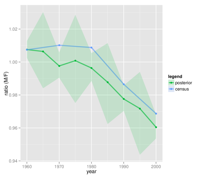
(a)

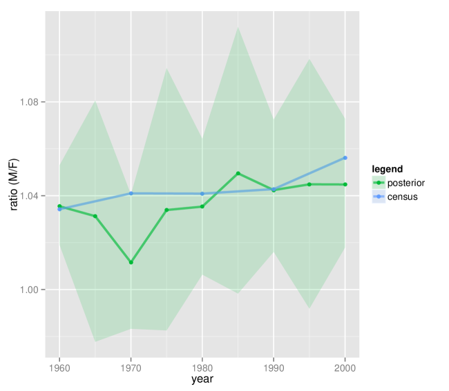
(b)

Figure 12: Prior and posterior medians and 95 percent credible intervals for the reconstructed population of Thailand, 1960–2000. Sex ratios (male/female) for LABEL:sub@fig:thai-res-prtp: total population; LABEL:sub@fig:thai-res-pr05: population aged 0–5; .

C.3 Laos

The results for U5MR are shown in Figure 13. Posterior median estimates of U5MR decreased. The posterior intervals for U5MR straddle one for the entire period of reconstruction (Figure 13c; mean half-width of the ratio 0.16). The probability that the male-to-female ratio of U5MR was less than one was 0.77 in 1985 but less than 0.2 in all other periods (Table 11). The probabilities of an increasing linear trend are given in Table 12.

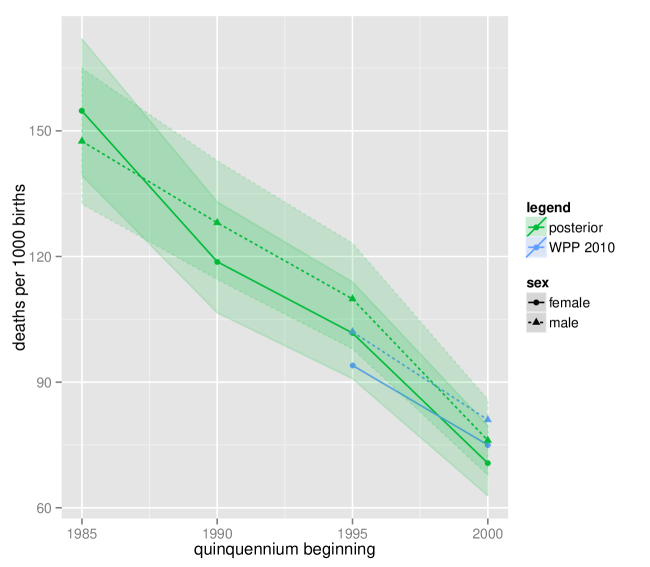
(a)

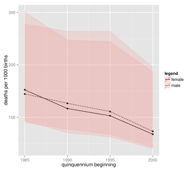
(b)

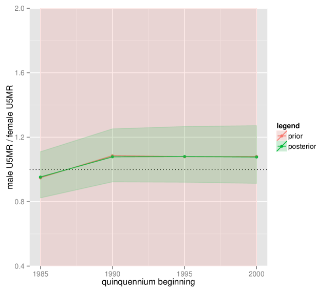
(c)

Figure 13: Prior and posterior medians and 95 percent credible intervals for under-five mortality rate (U5MR)(deaths per 1,000 live births) for the reconstructed population of Laos, 1985–2004. LABEL:sub@fig:laos-res-IMR-femaleVSmale: Female and male posterior quantiles and World Population Prospects (WPP)2010 estimates; LABEL:sub@fig:laos-res-IMR-femaleVSmale-prior: Female and male prior quantiles only; LABEL:sub@fig:laos-res-IMR-female-male-ratio: Male-to-female ratio.

Table 11: Probability that sex ratio of under-five mortality rate (SRU5MR)was less than one for the reconstructed population of Loas, 1985–2005, by quinquennium.

1985	1990	1995	2005
0.77	0.14	0.14	0.16

Table 12: Probabilities of an increasing linear trend and 95 percent credible intervals for sex ratio of under-five mortality rate (SRU5MR)for the reconstructed population of Laos, 1985–2000. Two measures of trend are used: the difference over the period of reconstruction and the slope coefficient from the ordinary least squares (OLS)regression on the start year of each quinquennium.

Measure of trend	95 percent CI	Prob $>$ 0
SRU5MR 2000 $-$ SRU5MR 1985	[$-$0.1, 0.35]	0.88
OLS slope (SRU5MR $\sim$ year)	[$-$0.0071, 0.022]	0.87

Posterior distributions for the average annual net number of migrants are shown in Figure 14. Posterior uncertainty is high, with a mean half-width of 8,890. Posterior medians indicate out-migration for most of the period of reconstruction. For 1995–2005, posterior intervals for males fall completely below zero.

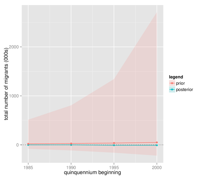
(a)

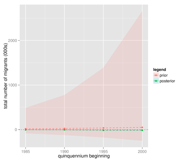
(b)

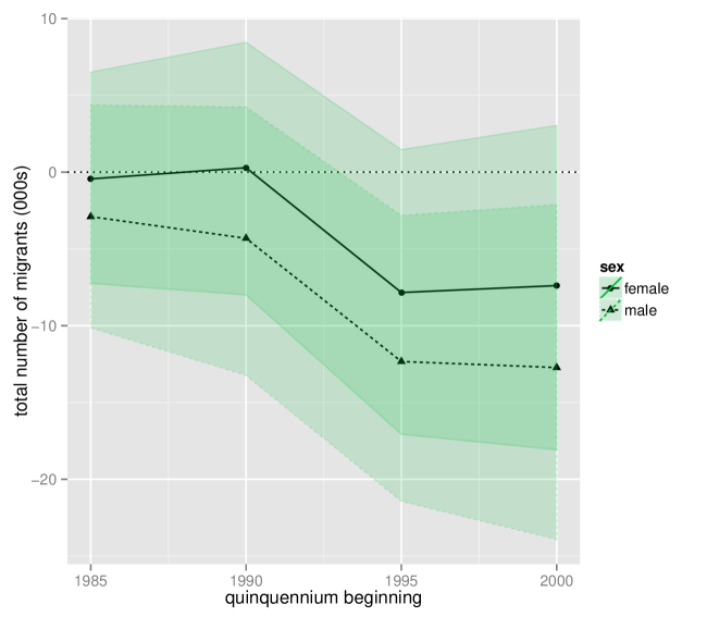
(c)

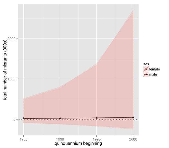
(d)

Figure 14: Prior and posterior medians and 95 percent credible intervals for the average annual net number of migrants for the reconstructed population of Laos, 1985–2004. LABEL:sub@fig:laos-res-totmig-female: Females; LABEL:sub@fig:laos-res-totmig-male: Males; LABEL:sub@fig:laos-res-totmig-femaleVSmale: Female and male posterior quantiles only; LABEL:sub@fig:laos-res-totmig-femaleVSmale-prior: Female and male prior quantiles only.

Posterior intervals for population sex ratios are in Figure 15. Posterior medians are reasonably similar to the ratios in the WPP census counts and uncertainty is high.

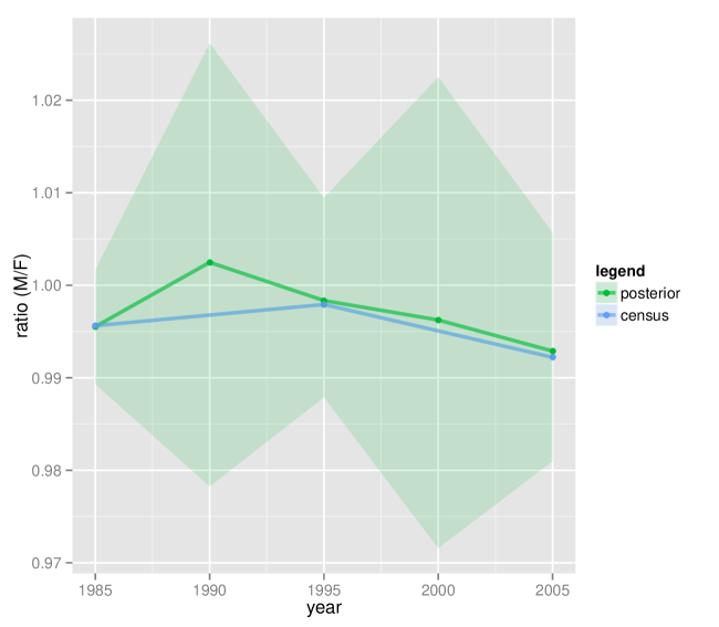
(a)

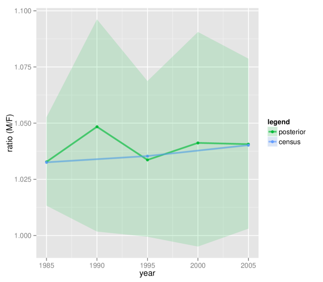
(b)

Figure 15: Prior and posterior medians and 95 percent credible intervals for the reconstructed population of Laos, 1985–2005. Sex ratios (male/female) for LABEL:sub@fig:laos-res-prtp: total population; LABEL:sub@fig:laos-res-pr05: population aged 0–5; .

Glossary

CCMPP

cohort component model of population projection

CD West

Coale and Demeny West

CEB

children ever born

CPS

Contraceptive Prevalence Survey

DHS

Demographic and Health Survey

e0

life expectancy at birth

IGME

Interagency Group for Child Mortality Estimation

MCMC

Markov chain Monte Carlo

NFHS

National Family Health Survey

OLS

ordinary least squares

RCHS

Reproductive and Child Health Survey

SDe0

sex difference in life expectancy at birth

SRB

sex ratio at birth

SRM

sex ratio of mortality

SRS

Sample Registration System

SRTP

sex ratio in the total population

SRU5

sex ratio in the population under five

SRU5MR

sex ratio of the under-five mortality rate

TFR

total fertility rate

U5MR

under-five mortality rate

UN

United Nations

UNPD

United Nations Population Division

vital rate

fertility and mortality rate

WFS

World Fertility Survey

WPP

World Population Prospects

References

- [1] Leontine Alkema and Wei Ling Ann “Estimating the Under-five Mortality Rate Using a Bayesian Hierarchical Time Series Model” In PLoS One 6.9 Public Library of Science, 2011, pp. e23954 DOI: 10.1371/journal.pone.0023954
- [2] Leontine Alkema, Adrian E. Raftery, Patrick Gerland, Samuel J. Clark and Francois Pelletier “Estimating Trends in the Total Fertility Rate with Uncertainty Using Imperfect Data: Examples from West Africa” In Demographic Research 26.15, 2012, pp. 331–362 DOI: 10.4054/DemRes.2012.26.15
- [3] E Arriaga “Estimating Fertility From Data on Children Ever Born by Age of Mother”, 1983
- [4] Steven N. Austad “Sex Differences in Longevity and Aging” In Handbook of the Biology of Aging Boston, Mass: Academic Press, 2011, pp. 479–495
- [5] “Inverse Projection Techniques: Old and New Approaches” In Inverse Projection Techniques: Old and New Approaches Berlin: Springer-Verlag, 2004
- [6] Joop Beer, James Raymer, Rob Erf and Leo Wissen “Overcoming the Problems of Inconsistent International Migration Data: A New Method Applied to Flows in Europe” In European Journal of Population/Revue Européenne de Démographie 26.4 Springer Netherlands, 2010, pp. 459–481 DOI: dx.doi.org/10.1007/s10680-010-9220-z
- [7] Neil G. Bennett and Shiro Horiuchi “Estimating the Completeness of Death Registration in a Closed Population” In Population Index 47.2 Office of Population Research, 1981, pp. 207–221 URL: http://www.jstor.org/stable/2736447
- [8] Salvatore Bertino and Eugenio Sonnino “The Stochastic Inverse Projection and the Population of Velletri (1590–1870)” In Mathematical Population Studies 10.1, 2003, pp. 41–73
- [9] P. N. Mari Bhat “Completeness of India’s Sample Registration System: An Assessment Using the General Growth Balance Method” In Population Studies 56.2 Taylor & Francis, Ltd. on behalf of the Population Investigation Committee, 2002, pp. 119–134 URL: http://www.jstor.org/stable/3092885
- [10] P. N. Mari Bhat “On the Trail of ‘Missing’ Indian Females I: Search for Clues” In Economic and Political Weekly 37.51 EconomicPolitical Weekly, 2002, pp. 5105–5118 URL: http://www.jstor.org/stable/4412986
- [11] P. N. Mari Bhat “On the Trail of ‘Missing’ Indian Females II: Illusion and Reality” In Economic and Political Weekly 37.52 EconomicPolitical Weekly, 2002, pp. 5244–5263 URL: http://www.jstor.org/stable/4413022
- [12] John Bongaarts “Fertility and Reproductive Preferences in Post-Transitional Societies” In Population and Development Review 27 Population Council, 2001, pp. 260–281 URL: http://www.jstor.org/stable/3115260
- [13] Phelim P. Boyle and Cormac Ó Gráda “Fertility Trends, Excess Mortality, and the Great Irish Famine” In Demography 23.4 Population Association of America, 1986, pp. 543–562 URL: http://www.jstor.org/stable/2061350
- [14] W Brass “The Demography of Tropical Africa” Princeton, NJ: Princeton University Press, 1968
- [15] William Brass “The Graduation of Fertility Distributions by Polynomial Functions” In Population Studies 14, 1960, pp. 148–162 URL: http://www.jstor.org/stable/2172011
- [16] William Brass “Uses of Census and Survey Data for the Estimation of Vital Rates”, 1964
- [17] William Brass and CELADE “Methods for Estimating Fertility and Mortality from Limited and Defective Data” Chapel Hill, North Carolina: Carolina Population Center, University of North Carolina at Chapel Hill, 1975
- [18] Aphichat Chamratrithirong, Pramote Prasartkul, Varachai Thongthai and Philip Guest “National Contraceptive Prevalence Survey 1996” Nakhon Pathom Thailand Mahidol University Institute for PopulationSocial Research (IPSR)., 1997
- [19] Ansley J. Coale “Excess Female Mortality and the Balance of the Sexes in the Population: An Estimate of the Number of Missing Females” In Population and Development Review 17, 1991, pp. 517–523
- [20] Ansley J. Coale, Paul Demeny and B. Vaughan “Regional Model Life Tables and Stable Populations” New York, New York: Academic Press, 1983
- [21] Joel E. Cohen “Stochastic Demography” Article Online Posting Date: August 15, 2006 In Encyclopedia of Statistical Sciences John WileySons, Inc., 2006 DOI: 10.1002/0471667196.ess2584.pub2
- [22] Beth Osborne Daponte, Joseph B. Kadane and Lara J. Wolfson “Bayesian Demography: Projecting the Iraqi Kurdish Population, 1977–1990” In Journal of the American Statistical Association 92.440 American Statistical Association, 1997, pp. 1256–1267 URL: http://www.jstor.org/stable/2965396
- [23] Monica Das Gupta “Explaining Asia’s “Missing Women”: A New Look at the Data” In Population and Development Review 31.3 Blackwell Publishing Ltd, 2005, pp. 529–535 DOI: 10.1111/j.1728-4457.2005.00082.x
- [24] Monica Das Gupta and P. N. Mari Bhat “Fertility Decline and Increased Manifestation of Sex Bias in India” In Population Studies 51.3, 1997, pp. 307–315
- [25] Griffith Feeney “A New Interpretation of Brass’ P/F Ratio Method Applicable When Fertility is Declining”, 1996 URL: http://www.heart-intl.net/HEART/HIV/Comp/InterpretationofFertiline.pdf
- [26] Carl M. Frisen “Population Characteristicsin the Lao People’s Democratic Republic” In Asia-Pacific Population Journal 6.2, 1991, pp. 55–66 URL: http://scholar.googleusercontent.com/scholar?q=cache:kW4rlEwV6OUJ:scholar.google.com/+Laos+fertility+sex+ratio+at+birth&hl=en&as_sdt=0,48
- [27] Daniel Goodkind and Loraine West “The North Korean Famine and its Demographic Impact” In Population and Development Review 27.2, 2001, pp. 219–238
- [28] T. N. E Greville “Short Methods for Constructing Model Life Tables” In The Record of the American Institute of Acturaries 32.65, 1943, pp. 29–42
- [29] Paula Griffiths, Zo e Matthews and Andrew Hinde “Understanding the Sex Ratio in India: A Simulation Approach” In Demography 37.4 Springer-Verlag, 2000, pp. 477–488 DOI: 10.1353/dem.2000.0004
- [30] Michel Guillot “The Dynamics of the Population Sex Ratio in India, 1971–96” In Population Studies 56.1 Taylor & Francis, Ltd. on behalf of the Population Investigation Committee, 2002, pp. 51–63 URL: http://www.jstor.org/stable/3092941
- [31] Christophe Z. Guilmoto “Characteristics of Sex-Ratio Imbalance in India and Future Scenarios”, 2007 URL: http://www.unfpa.org/gender/docs/studies/india.pdf
- [32] Christophe Z. Guilmoto “Characteristics of Sex-Ratio Imbalance in India and Future Scenarios: Executive Summary”, 2007 URL: http://www.unfpa.org/gender/docs/studies/summaries/india_summary.pdf
- [33] Christophe Z. Guilmoto “Sex Ratio Imbalance in Asia: Trends, Consequences and Policy Responses”, 2007 URL: http://www.unfpa.org/gender/docs/studies/summaries/regional_analysis.pdf
- [34] Christophe Z. Guilmoto “The Sex Ratio Transition in Asia” In Population and Development Review 35.3 Blackwell Publishing Ltd, 2009, pp. 519–549 DOI: 10.1111/j.1728-4457.2009.00295.x
- [35] Christophe Z. Guilmoto “Skewed Sex Ratios at Birth and Future Marriage Squeeze in China and India 2005–2100” In Demography 49, 2012, pp. 77–100
- [36] Patrick Heuveline “‘Between One and Three Million’: Towards the Demographic Reconstruction of a Decade of Cambodian History (1970–79).” In Population Studies 52, 1998, pp. 49–65
- [37] Kenneth Hill “Estimating Census and Death Registration Completeness” In Asian and Pacific Population Forum 1, 1987, pp. 8–13
- [38] Kenneth Hill, Patama Vapattanawong, Pramote Prasartkul, Yawarat Porapakkham, Stephen S Lim and Alan D Lopez “Epidemiologic Transition Interrupted: A Reassessment of Mortality Trends in Thailand, 1980–2000” In International Journal of Epidemiology 36.2, 2007, pp. 374–384 DOI: 10.1093/ije/dyl257
- [39] Kenneth Hill, Danzhen You, Mie Inoue, Mikkel Z. Oestergaard and Technical Advisory Group of the United Nations Inter-agency Group for˙Child Mortality Estimation (IGME) “Child Mortality Estimation: Accelerated Progress in Reducing Global Child Mortality, 1990–2010” In PLoS Medicine 9.8 Public Library of Science, 2012, pp. e1001303 DOI: 10.1371/journal.pmed.1001303
- [40] D. V. Hinkley “Inference About the Intersection in Two-Phase Regression” In Biometrika 56.3, 1969, pp. 495–504 URL: http://www.jstor.org/stable/2334655?origin=JSTOR-on-page
- [41] David V. Hinkley “Inference in Two-Phase Regression” In Journal of the American Statistical Association 66.336, 1971, pp. 736–743 URL: http://www.jstor.org/stable/2284220?origin=JSTOR-on-page
- [42] Prabhat Jha, Rajesh Kumar, Priya Vasa, Neeraj Dhingra, Deva Thiruchelvam and Rahim Moineddin “Low Male-to-female Sex Ratio of Children Born in India: National Survey of 1.1 Million Households” In The Lancet 367.9506, 2006, pp. 211–218 DOI: 10.1016/S0140-6736(06)67930-0
- [43] Prabhat Jha, Rajesh Kumar and Neeraj Dhingra “Sex Ratio in India — Authors’ Reply” In The Lancet 367.9524, 2006, pp. 1727 DOI: 10.1016/S0140-6736(06)68761-8
- [44] Prabhat Jha, Maya A. Kesler, Rajesh Kumar, Faujdar Ram, Usha Ram, Lukasz Aleksandrowicz, Diego G. Bassani, Shailaja Chandra and Jayant K. Banthia “Trends in Selective Abortions of Girls in India: Analysis of Nationally Representative Birth Histories from 1990 to 2005 and Census Data from 1991 to 2011” In The Lancet 377, 2011, pp. 1921–1928
- [45] Peerasit Kamnuansilpa, Aphichat Chamratrithirong and John Knodel “Thailand’s Reproductive Revolution: An Update” In International Family Planning Perspectives 8.2 Guttmacher Institute, 1982, pp. 51–56 URL: http://www.jstor.org/stable/2948088
- [46] Nathan Keyfitz and Hal Caswell “Applied Mathematical Demography”, Statistics for Biology and Health Springer, 2005
- [47] J. Knodel “Thailand’s Reproductive Revolution” In Social Science 72.1, 1987, pp. 52–56
- [48] John Knodel and Pichit Pitaktepsombati “Fertility and Family Planning in Thailand: Results from Two Rounds of a National Study” In Studies in Family Planning 6.11, 1975, pp. 402–413
- [49] John Knodel and Visid Prachuabmoh “Preferences for Sex of Children in Thailand: A Comparison of Husbands’ and Wives’ Attitudes” In Studies in Family Planning 7.5 Population Council, 1976, pp. 137–143 URL: http://www.jstor.org/stable/1964858
- [50] John Knodel, Vipan Prachuabmoh Ruffolo, Pakamas Ratanalangkarn and Kua Wongboonsin “Reproductive Preferences and Fertility Trends in Post-transition Thailand” In Studies in Family Planning 27.6 Population Council, 1996, pp. 307–318 URL: http://www.jstor.org/stable/2138026
- [51] Nevena Lalic and Adrian Elmes Raftery “Joint Probabilistic Projection of Female and Male Life Expectancy” In Proceedings of the Annual Meeting of the Population Association of America, 2012 URL: http://paa2012.princeton.edu/abstracts/120140
- [52] Ronald D. Lee “Reflections on Inverse Projection: Its Origins, Development, Extensions, and Relation to Forecasting” In Mathematical Population Studies 10.1, 2003, pp. 1–9
- [53] Ronald Demos Lee “Econometric Studies of Topics in Demographic History”, 1971
- [54] Ronald Demos Lee “Estimating Series of Vital Rates and Age Structures from Baptisms and Burials: A New Technique, with Applications to Pre-Industrial England” In Population Studies 28.3 Population Investigation Committee, 1974, pp. 495–512 URL: http://www.jstor.org/stable/2173642
- [55] P. H. Leslie “On the Use of Matrices in Certain Population Mathematics” In Biometrika 33.3 Biometrika Trust, 1945, pp. 183–212 URL: http://www.jstor.org/stable/2332297
- [56] P. H. Leslie “Some Further Notes on the Use of Matrices in Population Mathematics” In Biometrika 35.3/4 Biometrika Trust, 1948, pp. 213–245 URL: http://www.jstor.org/stable/2332342
- [57] Norman Y Luther and Robert D Retherford “Consistent Correction of Census and Vital Registration Data” In Mathematical Population Studies 1, 1988, pp. 1–20
- [58] Norman Y. Luther, Neramit Dhanasakdi and Fred Arnold “Consistent Correction of Census and Vital Registration Data for Thailand, 1960–80” Honolulu, Hawaii: East-West Population Institute, 1986
- [59] Prasanta Mahapatra “An Overview of the Sample Registration System in India” In Prince Mahidol Award Conference & Global Health Information Forum, 2010 URL: http://unstats.un.org/unsd/vitalstatkb/KnowledgebaseArticle50447.aspx
- [60] Peter Mayer “India’s Falling Sex Ratios” In Population and Development Review 25.2 Population Council, 1999, pp. 323–343 URL: http://www.jstor.org/stable/172428
- [61] M. Giovanna Merli “Mortality in Vietnam, 1979-1989” In Demography 35.3 Population Association of America, 1998, pp. 345–360 URL: http://www.jstor.org/stable/3004042
- [62] C. J. L. Murray, B. D. Ferguson, A. D. Lopez, M. Guillot, J. A. Salomon and O. Ahmad “Modified Logit Life Table System: Principles, Empirical Validation, and Application” In Population Studies 57.2 Population Investigation Committee, 2003, pp. 165–182 URL: http://www.jstor.org/stable/3595746
- [63] Christopher J. L. Murray, Julie Knoll Rajaratnam, Jacob Marcus, Thomas Laakso and Alan D. Lopez “What Can We Conclude from Death Registration? Improved Methods for Evaluating Completeness” In PLoS Med 7.4 Public Library of Science, 2010, pp. e1000262 DOI: 10.1371/journal.pmed.1000262
- [64] National Research Council Panel on Thailand “Fertility and Mortality Changes in Thailand, 1950–1975”, Report (National Research Council. Committee on Population and Demography) Washington, D.C.: National Academy of Sciences, 1980
- [65] James Oeppen “Back Projection and Inverse Projection: Members of a Wider Class of Constrained Projection Models” In Population Studies 47.2 Population Investigation Committee, 1993, pp. 245–267 URL: http://www.jstor.org/stable/2174729
- [66] James Oeppen “Generalized Inverse Projection” In Old and New Methods in Historical Demography Oxford, England: Clarendon Press, 1993, pp. 29–39
- [67] J. H. Pollard “A Note on Multi-Type Galton-Watson Processes with Random Branching Probabilities” In Biometrika 55.3 Biometrika Trust, 1968, pp. 589–590 URL: http://www.jstor.org/stable/2334271
- [68] Ronald Pongou “Why Is Infant Mortality Higher in Boys Than in Girls? A New Hypothesis Based on Preconception Environment and Evidence From a Large Sample of Twins” In Demography 50, 2013, pp. 421–444 DOI: 10.1007/s13524-012-0161-5
- [69] Samuel H. Preston “Mortality Patterns in National Populations” New York, New York: Academic Press, 1976
- [70] Samuel H. Preston, Patrick Heuveline and Michel Guillot “Demography: Measuring and Modeling Population Processes” Malden, Massachusetts: Blackwell, 2001
- [71] R Core Team “R: A Language and Environment for Statistical Computing”, 2013 R Foundation for Statistical Computing URL: http://www.R-project.org/
- [72] Adrian E Raftery and Steven M Lewis “Implementing MCMC” In Markov Chain Monte Carlo in Practice London: Chapman & Hall, 1996, pp. 115–130
- [73] Cheryl Chriss Sawyer “Child Mortality Estimation: Estimating Sex Differences in Childhood Mortality since the 1970s” In PLoS Med 9.8 Public Library of Science, 2012, pp. e1001287 DOI: 10.1371/journal.pmed.1001287
- [74] Amartya Sen “More Than 100 Million Women are Missing” In New York Review of Books 20, 1990, pp. 61–66
- [75] Romesh Silva “Child Mortality Estimation: Consistency of Under-Five Mortality Rate Estimates Using Full Birth Histories and Summary Birth Histories” In PLoS Medicine 9.8 Public Library of Science, 2012, pp. e1001296 DOI: 10.1371/journal.pmed.1001296
- [76] Lamberto Soliani and Enzo Luchetti “Genetic Factors in Mortality” Burlington, MA: Academic Press, 2006, pp. 117–128
- [77] Titaya Suvanajata and Peerasit Kamnuansilpa “Thailand Contraceptive Prevalence Survey: Country Report” Bangkok, Thailand: Research Center, National Institute of Development Administration, 1979
- [78] The National Statistical Office of Thailand “Report: The Survey of Population Change, 1964–67” The National Statistical Office of Thailand, 1970 The Government of Thailand
- [79] The National Statistical Office of Thailand “Report: The Survey of Population Change, 1974–1975” The National Statistical Office of Thailand, 1977 The Government of Thailand
- [80] The National Statistical Office of Thailand “Report, The Survey of Population Change, 1991” Bangkok, Thailand: The National Statistical Office of Thailand, 1992 The Government of Thailand
- [81] The National Statistical Office of Thailand “Report on The 1995–1996 Survey of Population Change” Bangkok, Thailand: The National Statistical Office of Thailand, 1997 The Government of Thailand
- [82] The Registrar General and Census Commissioner of India “National Family Health Survey, India”, 2009 Misitry of Home Affairs, The Government of India URL: http://censusindia.gov.in/Vital_Statistics/SRS/Sample_Registration_System.aspx
- [83] The Registrar General and Census Commissioner of India “Vital Statistics: Sample Registration”, 2011 Misitry of Home Affairs, The Government of India URL: http://censusindia.gov.in/Vital_Statistics/SRS/Sample_Registration_System.aspx
- [84] United Nations “Model Life Tables for Developing Countries”, Population Studies (Department of International, Economic and Social Affairs) 77 New York, New York: United Nations, Sales No. E.07.XIII.7, 1982
- [85] United Nations “Manual X: Indirect Techniques for Demographic Estimation”, Population Studies (Department of International, Economic and Social Affairs) 81 New York, NY: United Nations, Sales No. E.83.XIII.2, 1983
- [86] United Nations “Fertility Levels and Trends as Assessed from Twenty World Fertility Surveys” New York, New York: United Nations, document number: ST/ESA/SER.R/50, 1993
- [87] United Nations “World Population Prospects: The 2010 Revision, Standard Variants (Updated: 28 June 2011)”, 2011 Department of Economic and Social Affairs (DESA), Population Division, Population Estimates and Projections Section URL: http://esa.un.org/unpd/wpp/index.htm
- [88] United Nations Population Fund “UNFPA Guidance Note on Sex Selection”, 2010 URL: http://www.unfpa.org/webdav/site/global/shared/documents/publications/2010/guidenote_prenatal_sexselection.pdf
- [89] Jacques Vallin “La Population de la Thailande” In Population (French Edition) 31.1 Institut National d’Études Démographiques, 1976, pp. 153–175 URL: http://www.jstor.org/stable/1531035
- [90] Jacques Vallin “Mortality, Sex, and Gender” Burlington, MA: Academic Press, 2006, pp. 177–194
- [91] Patama Vapattanawong and Pramote Prasartkul “Under-Registration of Deaths in Thailand in 2005–2006: Results of Cross-Matching Data from Two Sources” In Bulletin of the World Health Organization 89.11, 2011, pp. 806–812 DOI: 10.2471/BLT.10.083931
- [92] Pravin M. Visaria “The Sex Ratio of the Population of India” 1.10, Census of India, Monographs New Delhi, India: Ministry of Home Affairs, Office of the Registrar General, 1971
- [93] Ingrid Waldron “What Do We Know About Causes of Sex Differences in Mortality? A Review of the Literature” In Population Bulletin of the United Nations 18, 1985, pp. 59–76
- [94] Ingrid Waldron “Gender Differences in Mortality—Causes and Variation in Different Societies” In The Sociology of Health and Illness: Critical Perspectives New York, New York: Worth, 2009, pp. 38–54
- [95] Sarah L. Walters “Fertility, Mortality and Marriage in Northwest Tanzania, 1920–1970: a Demographic Study Using Parish Registers”, 2008
- [96] Mark Christopher Wheldon, Adrian Elmes Raftery, Samuel J. Clark and Patrick Gerland “Bayesian Reconstruction of Past Populations and Vital Rates by Age for Developing and Developed Countries”, 2013 Population Association of America URL: http://paa2013.princeton.edu/abstracts/130303
- [97] Mark Christopher Wheldon, Adrian Elmes Raftery, Samuel J. Clark and Patrick Gerland “Reconstructing Past Populations with Uncertainty from Fragmentary Data” In Journal of the American Statistical Association 108.501, 2013, pp. 96–110 DOI: 10.1080/01621459.2012.737729
- [98] P. K. Whelpton “An Empirical Method of Calculating Future Population” In Journal of the American Statistical Association 31.195 American Statistical Association, 1936, pp. 457–473 URL: http://www.jstor.org/stable/2278370
- [99] Edward Anthony Wrigley and Roger S. Schofield “The Population History of England, 1541–1871: A Reconstruction”, Studies in Social and Demographic History London, England: Edward Arnold, 1981
- [100] B. Zaba “Use of the Relational Gompertz Model in Analysing Fertility Data Collected in Retrospective Surveys”, 1981