On plane-wave relativistic electrodynamics in plasmas and in vacuum

Abstract

We revisit the exact microscopic equations (in differential, and equivalent integral form) ruling a relativistic cold plasma after the plane-wave Ansatz, without customary approximations. We show that in the Eulerian description the motion of a very diluted plasma initially at rest and excited by an arbitrary transverse plane electromagnetic travelling-wave has a very simple and explicit dependence on the transverse electromagnetic potential; for a non-zero density plasma the above motion is a good approximation of the real one as long as the back-reaction of the charges on the electromagnetic field can be neglected, i.e. for a time lapse decreasing with the plasma density, and can be used as initial step in an iterative resolution scheme.

As one of many possible applications, we use these results to describe how the ponderomotive force of a very intense and short plane laser pulse hitting normally the surface of a plasma boosts the surface electrons into the ion background. Because of this penetration the electrons are then pulled back by the electric force exerted by the ions and may leave the plasma with high energy in the direction opposite to that of propagation of the pulse [G. Fiore, R. Fedele, U. De Angelis, The slingshot effect: a possible new laser-driven high energy acceleration mechanism for electrons, arXiv:1309.1400].

1 Introduction

Consider a charged test particle initially at rest. The solution ${\bm{x}}(t,{\bm{X}})$ of its equation of motion under the action of a given electromagnetic (EM) field is a function of the time $t$ and of the initial position ${\bm{X}}$. By definition a charged test particle has such a small electric charge that its influence on the EM field can be neglected. This is of course an idealization of real particles, but actually an extremely good one for microscopic particles (electrons, ions, etc) under the action of macroscopic EM fields. If we imagine to fill at the initial time a region ${\cal B}$ with a “very diluted” fluid of test particles of the same kind at rest, then the function ${\bm{x}}(t,{\bm{X}})$ will describe the motion of such a fluid under the action of the given EM field. ${\bm{X}}\!\in\!{\cal B}$ will be used as a label to distinguish the single particles composing the fluid (Lagrangian description): ${\bm{x}}(t,{\bm{X}})$ [more generally, a function $\tilde{f}(t,{\bm{X}})$)] will give the position (more generally, the fluid observable $f$) at time $t$ of the particle (or better, fluid element) initially located at ${\bm{X}}$. By definition, the fluid just described will have zero density and be initially at rest; this motivates us in the first place to study its equation of motion in a given (necessarily free) EM field. If the free EM field is an arbitrary transverse plane travelling-wave with a (whether smooth or sharp) front, then the solution has a very simple expression (subsection 2.3) in terms of the EM field (it is completely explicit apart from the inversion of a strictly increasing function $\Xi(\xi)$ of one variable $\xi$). We prove this result going from the Lagrangian to the Eulerian description, and back. The motion of a single test particle with non-zero initial velocity is obtained from that with zero initial velocity by a suitable Poincaré transformation. These results agree with the motion (in implicit form) of the particle obtained by resolution of its Hamilton-Jacobi equation [2] (see e.g. also [3, 4]).

One can combine several such fluids into a cold plasma, and ask whether and how well these zero-density solutions approximate the solutions of the (coupled) Lorentz-Maxwell and continuity equations (subsection 2.1) for non-zero densities with the same plane symmetry and asymptotic conditions (subsection 2.2). In section 3 in full generality we solve for the longitudinal electric field in terms of the longitudinal coordinates of the particles and formulate integral equations equivalent to the remaining differential equations. In [5] we will discuss a recursive resolution scheme for these integral equations in which the zero-density solutions play the role of lowest order approximations. In section 4 we just determine the first correction for a EM wave hitting a step-shaped density plasma and show for how long this correction is small. As an illustration, in section 4.1 we use these results to determine conditions under which the slingshot effect [1] may occur.

Up to section 3 no role is played by Fourier analysis and related methods/notions, such as the Slowly Varying Amplitude Approximation [6, 7, 8], (frequency-dependent) refractive indices [9, 10], etc. Our scope here is to derive from the basic microscopic equations some general results which can be used, at least for a limited time lapse, also in the presence of very intense EM waves with completely arbitrary profile (we do not assume existence of a carrier frequency nor of a slowly varying envelope amplitude), when the methods mentioned above become inadequate. These conditions, which involve fast and highly nonlinear effects, characterize important plasma phenomena in current laboratory research on laser-plasma interactions, such as Laser Wake Field excitations and acceleration [11, 12, 13] (with external [14] or self injection [15]; for a short list of their applications see also the introduction of[16]), especially in the bubble (or blowout) regime [17, 18, 19], or the propagation of intense laser beams through overdense plasmas [20, 21], etc. (see e.g. [22]). Only in section 4 we specialize calculations to a very intense laser pulse with a (not so slowly) varying envelope.

2 Preliminaries

2.1 Cold plasma equations

We first recall the basic plasma equations and some basic facts about fluid mechanics, while fixing the notation. We consider a collisionless plasma composed by $k\geq 2$ types of charged particles (electrons, ions of various kinds, etc). For $h\!=\!1,...,k$ we denote by $m_{h},q_{h}$ the rest mass and charge of the $h$-th type of particle, by ${\bm{v}}_{h}({\bm{x}},ct)$, $n_{h}({\bm{x}},ct)$ respectively the 3-velocity and the density (number of particles - treated as usual as a continuous rather than an integer-valued variable - per unit volume) of the corresponding fluid element located in position ${\bm{x}}$ at time $t$ ($c$ is the light velocity). It is convenient to formulate the equations in terms of dimensionless unknowns like  ${\bm{\beta}}_{h}\!:=\!{\bm{v}}_{h}/c$, $\gamma_{h}\!:=\!1/\sqrt{1\!-\!{\bm{\beta}}_{h}^{2}}$,  the 4-velocity of the $h$-th type of particle  $(u_{h}^{\mu})\!:=\!(\gamma_{h},\gamma_{h}{\bm{\beta}}_{h})$.  The latter is normalized,  $u_{h}^{\mu}u_{h\mu}\!=\!1$  (indices are raised and lowered by the Minkowski metric $\eta_{\mu\nu}\!=\!\eta^{\mu\nu}$, with $\eta^{00}\!=\!1$, $\eta^{11}\!=\!-1$, etc.), implying $\gamma_{h}\!=\!u_{h}^{0}\!=\!\sqrt{1\!+\!{\bm{u}}_{h}^{2}}$, ${\bm{\beta}}_{h}\!=\!{\bm{u}}_{h}/\gamma_{h}$; $u_{h}^{\mu}$ is essentially the 4-momentum $(p^{\mu}_{h})=(p_{h}^{0},{\bm{p}}_{h})$ of the $h$-th type of particles made dimensionless by dividing by the appropriate powers of $m_{h},c$:  $\gamma_{h}\!=\!u_{h}^{0}\!=\!p^{0}_{h}/m_{h}c^{2}$,  ${\bm{u}}_{h}\!=\!\mbox{\boldmath$p$}_{h}/m_{h}c$.  The 4-vector current density  $(j^{\mu})=(j^{0},{\bm{j}})$ is now given by $j^{0}\!=\!\sum_{h=1}^{k}q_{h}n_{h}$,  ${\bm{j}}\!=\!\sum_{h=1}^{k}q_{h}n_{h}{\bm{v}}_{h}/c\!=\!\sum_{h=1}^{k}q_{h}n_{h}{\bm{\beta}}_{h}$.

We use the CGS system. As usual, we denote by $(A^{\mu})=(A^{0},{\bm{A}})$ the electromagnetic potential, by $F^{\mu\nu}=\partial^{\mu}A^{\nu}-\partial^{\nu}A^{\mu}$ the electromagnetic field, where $x=(x^{\mu})=(x^{0},{\bm{x}})=(ct,{\bm{x}})$, $(\partial_{\mu})\equiv(\partial/\partial x^{\mu})=(\partial_{0},\nabla)$. We start from the explicitly Lorentz-covariant formulation of the Maxwell’s equations and of the Lorentz equations of motion of the collisionless fluids:

$$\Box A^{\nu}-\partial^{\nu}(\partial_{\mu}A^{\mu})=\partial_{\mu}F^{\mu\nu}=4\pi j^{\nu},$$ (1)

$$-q_{h}u_{h\mu}F^{\mu\nu}=m_{h}c^{2}u_{h\mu}\partial^{\mu}u_{h}^{\nu}\qquad h=1,...,k;$$ (2)

the unknowns are $A^{\mu},n_{h},{\bm{u}}_{h}$,  $h=1,...,k$. [As known, the component $\nu=0$ of (2) is not independent of the other ones; it can be obtained contracting the components $\nu=l=1,2,3$ with $u^{l}_{h}$ and using the definitions above]. Dividing the components $\nu=l$ by $\gamma_{h}$ and using the definitions $E^{l}=F^{l0}=-\partial_{0}A^{l}-\partial_{l}A^{0}$, $B^{l}=-\frac{1}{2}\varepsilon^{lkn}F^{kn}=\varepsilon^{lkn}\partial_{k}A^{n}$ of the electric and magnetic field one obtains the equivalent, familiar 3-vector formulation of (2)

$$q_{h}\left({\bm{E}}+\frac{{\bm{v}}_{h}}{c}\wedge{\bm{B}}\right)=\partial_{t}{\bm{p}}_{h}+{\bm{v}}_{h}\cdot\nabla{\bm{p}}_{h}=\frac{d{\bm{p}}_{h}}{dt},\qquad\qquad{\bm{p}}_{h}=m_{h}\gamma_{h}{\bm{v}}_{h}.$$ (3)

In the second equality we have used the relation between the total (or material) derivative $\frac{d}{dt}$ for the $h$-th type of particle and $\partial_{\mu}$, ${\bm{v}}_{h}$:

$$\frac{d}{dt}:=\partial_{t}\!+\!v^{l}_{h}\partial_{l}\qquad\qquad\Leftrightarrow\qquad\qquad\frac{d}{dx^{0}}:=\partial_{0}\!+\!\beta^{l}_{h}\partial_{l}=\frac{u_{h}^{\mu}}{\gamma_{h}}\partial_{\mu}.$$ (4)

Eq. (2) are formulated in the Eulerian description: the volume element of the $h$-th fluid is labelled by its position ${\bm{x}}$ at time $x^{0}=ct$, and all the observables are described as functions of $(x^{0},{\bm{x}})$. Given an observable $f_{h}(x^{0},{\bm{x}})$ of the $h$-th fluid in the Eulerian description, it is related to its Lagrangian counterpart $\tilde{f}_{h}(x^{0},{\bm{X}})$ by

$$\tilde{f}_{h}(x^{0},{\bm{X}})=f_{h}[x^{0},{\bm{x}}_{h}(x^{0},{\bm{X}})]\qquad\Leftrightarrow\qquad f_{h}(x^{0},{\bm{x}})=\tilde{f}_{h}[x^{0},{\bm{X}}_{h}({\bm{x}},x^{0})];$$ (5)

here ${\bm{x}}_{h}(x^{0},{\bm{X}})$ is the position at time $x^{0}=ct$ of the $h$-th fluid element initially located in ${\bm{X}}$, and ${\bm{X}}_{h}(x^{0},{\bm{x}})$ is its inverse (for fixed $x^{0}$), i.e. the initial position of the $h$-th fluid element located in ${\bm{x}}$ at time $x^{0}=ct$; by construction ${\bm{X}}_{h}(X^{0},{\bm{x}})={\bm{x}}$. The correspondences  ${\bm{x}}_{h}(x^{0},\cdot):{\bm{X}}\mapsto{\bm{x}}$  and  ${\bm{X}}_{h}(x^{0},\cdot):{\bm{x}}\mapsto{\bm{X}}$  are required to be one-to-one and to have continuous first derivatives (so the Jacobian $\tilde{J}_{h}:=\det\|\frac{\partial{\bm{x}}_{h}}{\partial{\bm{X}}}\|$ as well as its inverse never vanish and reduce to 1 at $x^{0}=X^{0}$) and continuous second derivatives with respect to time (at least piecewise). Clearly, $J_{h}=\det^{-1}\|\frac{\partial{\bm{X}}_{h}}{\partial{\bm{x}}}\|$. By construction, $f_{h}(X^{0},{\bm{x}})\!=\!\tilde{f}_{h}(X^{0},{\bm{x}})\!=:\!\tilde{f}_{h0}({\bm{x}})$, where $X^{0}$ is the initial time. In the Lagrangian and Eulerian description the conservation of the number of particles of the $h$-th fluid in each material volume element of volume $d^{3}x$ respectively amounts to

$$\tilde{n}_{h}(x^{0},{\bm{X}})\tilde{J}_{h}(x^{0},{\bm{X}})=\widetilde{n_{h0}}({\bm{X}})\qquad\qquad\Leftrightarrow\qquad\qquad n_{h}(x^{0},{\bm{x}})J_{h}(x^{0},{\bm{x}})_{h0}(x^{0},{\bm{x}}).$$ (6)

$\widetilde{n_{h0}}$ is $\widetilde{n_{h}}$ evaluated at the time $x^{0}=X^{0}$; it is part of the initial data. As known, $\frac{d}{dt}$ becomes the partial derivative $\partial_{t}$ (or equivalently, $\frac{d}{dx^{0}}$ becomes $\partial_{0}$) when going from the Eulerian to the Lagrangian description. The continuity equation of the $h$-th fluid follows from (6) and $\partial_{0}\widetilde{n_{h0}}=0$, and reads

$$\partial_{0}(\tilde{n}_{h}\tilde{J}_{h})=0,\qquad\qquad\Leftrightarrow\qquad\qquad\frac{dn_{h}}{dx^{0}}\!+\!n_{h}\nabla\!\cdot\!{\bm{\beta}}_{h}=\partial_{0}n_{h}\!+\!\nabla\!\cdot\!(n_{h}{\bm{\beta}}_{h})=0.$$ (7)

The equivalence in (7) is based on the well-known identity $\frac{dJ_{h}}{dx^{0}}=J_{h}\nabla\!\cdot\!{\bm{\beta}}_{h}.$ Eq. (1) implies the electric current conservation law $\partial_{\mu}j^{\mu}=0$, what makes one of the $k$ conservation laws (7) redundant. From the definition $\widetilde{\bm{v}}_{h}(ct,{\bm{X}}):=\partial_{t}{\bm{x}}_{h}(ct,{\bm{X}})$, or equivalently $\widetilde{\bm{\beta}}_{h}(x^{0},{\bm{X}}):=\partial_{0}{\bm{x}}_{h}(x^{0},{\bm{X}})$, it follows that if the function ${\bm{\beta}}_{h}(x^{0},{\bm{x}})$ is known one can determine the maps ${\bm{x}}_{h}:{\bm{X}}\mapsto{\bm{x}}$ by solving the Cauchy problems

$$\partial_{0}{\bm{x}}_{h}(x^{0},{\bm{X}})={\bm{\beta}}_{h}\!\left[{x^{0}},{\bm{x}}_{h}({x^{0}},{\bm{X}})\right]$$ (8)

with initial conditions ${\bm{x}}_{h}(X^{0},{\bm{X}})\!=\!{\bm{X}}$. If all the observables $f_{h}$ admit for all ${\bm{x}}$ finite limits $\lim_{x^{0}\to-\infty}f_{h}(x^{0},{\bm{x}})\!=:\!\tilde{f}_{h0}({\bm{x}})$ and in particular $\tilde{\bm{\beta}}_{h0}({\bm{x}})\!\equiv\!{\bf 0}$, then one may use also $X^{0}\!=\!-\infty$ as ‘initial’ time, and as ‘initial’ conditions the corresponding asymptotic ones, e.g. for each ${\bm{X}}$ the condition ${\bm{x}}_{h}(x^{0},{\bm{X}})\!\to\!{\bm{X}}$ as $x^{0}\!\to\!-\infty$ to complement (8).

2.2 Cold plasma equations for plane waves with a front

Henceforth we restrict our attention to solutions of (1-3), (6-8) such that for all $h$:

$$A^{\mu},n_{h},{\bm{u}}_{h}\qquad\mbox{{\bf depend only on }}z\!\equiv\!x^{3}\!,x^{0}\qquad\mbox{(plane wave Ansatz)},$$ (9)

$$\!\!\begin{array}[]{ll}A^{\mu}(x^{0}\!,z)\!=\!0,\qquad{\bm{u}}_{h}(x^{0}\!,z)\!=\!{\bf 0},&\qquad\qquad\mbox{if }\>\>x^{0}\!\leq\!z,\\[4.0pt] \exists\>\>\widetilde{n_{h0}}(z)\qquad\mbox{such that }\>\displaystyle\sum_{h=1}^{k}\!q_{h}\widetilde{n_{h0}}\!\equiv\!0,\qquad n_{h}(x^{0}\!\!,z)\!=\!\widetilde{n_{h0}}(z)&\qquad\qquad\mbox{if }\>\>x^{0}\!\leq\!z.\end{array}\qquad$$ (12)

These equations (which entail a partial gauge-fixing) imply

$${\bm{B}}\!=\!{\bm{B}}^{{\scriptscriptstyle\perp}}\!=\!{\hat{\bm{z}}}\!\wedge\!\partial_{z}{\bm{A}}\!^{{\scriptscriptstyle\perp}},\qquad\qquad\qquad{\bm{E}}^{{\scriptscriptstyle\perp}}\!=\!-\partial_{0}{\bm{A}}\!^{{\scriptscriptstyle\perp}},\qquad$$ (13)

$${\bm{E}}(x^{0}\!,z)={\bm{B}}(x^{0}\!,z)={\bf 0}\qquad\qquad{\bm{x}}_{h}(x^{0}\!,{\bm{x}})={\bm{x}}\qquad\qquad\qquad\mbox{if }\>\>x^{0}\leq z,\qquad$$ (14)

and are fulfilled, after a suitable $z$-translation, by any plasma initially neutral and at equilibrium with purely $z$-dependent densities $\widetilde{n_{h0}}(z)$ in a zero electromagnetic field and then reached by a purely transverse electromagnetic wave (with a front) propagating from infinity in the positive $z$ direction. Of course, our results will be applicable also if conditions (9-12) can be achieved by a Poincaré transformation. Equations (12)₃, (14)₂ trivially imply  $n_{h}(-\infty,Z)\!=\!\widetilde{n_{h0}}(Z)$,  ${\bm{x}}_{h}(-\infty,{\bm{X}})\!=\!{\bm{X}}$.   Therefore we can adopt also the configuration of the plasma at the ‘initial’ time $X^{0}\!=\!-\infty$ as a reference configuration in the Lagrangian description.

${\bm{A}}\!^{{\scriptscriptstyle\perp}}$ has become a physical observable, as it can be recovered from ${\bm{E}}^{{\scriptscriptstyle\perp}}$ integrating (13)₁ with respect to $x^{0}$ at fixed $z$ and exploiting (12): $-{\bm{A}}\!^{{\scriptscriptstyle\perp}}(x^{0},z)=\!\int^{x^{0}}_{z}\!\!\!\!dx^{0}{}^{\prime}\,{\bm{E}}^{{\scriptscriptstyle\perp}}(x^{0}{}^{\prime},z)=\!\int^{x^{0}}_{-\infty}\!\!\!\!dx^{0}{}^{\prime}\,{\bm{E}}^{{\scriptscriptstyle\perp}}(x^{0}{}^{\prime},z)$.

Eq. (2)_ν=x,y implies

$$\qquad\qquad\qquad u_{h}^{\mu}\partial_{\mu}\!\left(m_{h}c^{2}{\bm{u}}_{h}^{{\scriptscriptstyle\perp}}\!+\!q_{h}{\bm{A}}\!^{{\scriptscriptstyle\perp}}\!\right)\!=\!\gamma_{h}\frac{d(m_{h}c^{2}{\bm{u}}_{h}^{{\scriptscriptstyle\perp}}\!+\!q_{h}{\bm{A}}\!^{{\scriptscriptstyle\perp}})}{dx^{0}}\!=\!0;$$

in the Lagrangian description this becomes $\partial_{0}(m_{h}c^{2}\tilde{{\bm{u}}}_{h}^{{\scriptscriptstyle\perp}}\!+\!q_{h}\widetilde{{\bm{A}}}\!^{{\scriptscriptstyle\perp}})=0$, implying that $m_{h}c^{2}\tilde{{\bm{u}}}_{h}^{{\scriptscriptstyle\perp}}\!+\!q_{h}\tilde{{\bm{A}}}\!^{{\scriptscriptstyle\perp}}=C({\bm{X}})=$const  with respect to $x^{0}$;  by (12)   $C({\bm{X}})\equiv 0$. Thus one obtains the known result

$$\tilde{{\bm{u}}}_{h}^{{\scriptscriptstyle\perp}}\!=\frac{-q_{h}}{m_{h}c^{2}}\tilde{{\bm{A}}}\!^{{\scriptscriptstyle\perp}}\qquad\Leftrightarrow\qquad{\bm{u}}_{h}^{{\scriptscriptstyle\perp}}\!=\frac{-q_{h}}{m_{h}c^{2}}{\bm{A}}\!^{{\scriptscriptstyle\perp}},$$ (15)

which explicitly gives ${\bm{u}}_{h}^{{\scriptscriptstyle\perp}}$ in terms of ${\bm{A}}\!^{{\scriptscriptstyle\perp}}$. Eq. (1) and the remaining (2) become

$$(\ref{Maxwell})_{\nu=0}:\qquad\partial_{z}E^{z}=4\pi\sum_{h=1}^{k}q_{h}n_{h},$$ (16)

$$(\ref{Maxwell})_{\nu=z}:\qquad\partial_{0}E^{z}=-\frac{4\pi}{c}\sum_{h=1}^{k}q_{h}n_{h}v^{z}_{h}=-4\pi\sum_{h=1}^{k}q_{h}n_{h}\beta^{z}_{h},$$ (17)

$$(\ref{Maxwell})_{\nu=x,y}:\quad\>\left(\partial_{0}^{2}\!-\!\partial_{z}^{2}\right)\!{\bm{A}}\!^{{\scriptscriptstyle\perp}}\!\!-\!4\pi\sum_{h=1}^{k}q_{h}n_{h}{\bm{\beta}}^{{\scriptscriptstyle\perp}}_{h}\stackrel{{\scriptstyle(\ref{hom'12})}}{{=}}\!\left[\partial_{0}^{2}\!-\!\partial_{z}^{2}\right]\!\!{\bm{A}}\!^{{\scriptscriptstyle\perp}}\!+\!\frac{4\pi}{c^{2}}\left[\sum_{h=1}^{k}\frac{q_{h}^{2}n_{h}}{m_{h}\gamma_{h}}\right]\!{\bm{A}}\!^{{\scriptscriptstyle\perp}}\!=0,\qquad\qquad$$ (18)

$$(\ref{hom'})_{\nu=0}:\qquad m_{h}c^{2}u_{h}^{\mu}\partial_{\mu}\gamma_{h}\!-\!q_{h}u^{z}_{h}E^{z}\!+\!q_{h}{\bm{u}}_{h}^{{\scriptscriptstyle\perp}}\cdot\partial_{0}{\bm{A}}\!^{{\scriptscriptstyle\perp}}\stackrel{{\scriptstyle(\ref{totder}),(\ref{hom'12})}}{{=}}m_{h}c^{2}\gamma_{h}\frac{d\gamma_{h}}{dx^{0}}\!-\!q_{h}u^{z}_{h}E^{z}$$

$$\qquad\qquad\qquad-\frac{q_{h}^{2}}{m_{h}c^{2}}{\bm{A}}\!^{{\scriptscriptstyle\perp}}\!\cdot\!\partial_{0}{\bm{A}}\!^{{\scriptscriptstyle\perp}}=0,\qquad\Leftrightarrow\qquad\frac{d\gamma_{h}}{dx^{0}}-\frac{q_{h}u^{z}_{h}E^{z}}{m_{h}c^{2}\gamma_{h}}-\frac{q_{h}^{2}\partial_{0}({\bm{A}}\!^{{\scriptscriptstyle\perp}})^{2}}{2\gamma_{h}m_{h}^{2}c^{4}}=0$$ (19)

$$(\ref{hom'})_{\nu=z}:\qquad m_{h}c^{2}u_{h}^{\mu}\partial_{\mu}u^{z}_{h}\!-\!q_{h}\gamma_{h}E^{z}\!-\!q_{h}{\bm{u}}_{h}^{{\scriptscriptstyle\perp}}\cdot\partial_{z}{\bm{A}}\!^{{\scriptscriptstyle\perp}}\stackrel{{\scriptstyle(\ref{totder}),(\ref{hom'12})}}{{=}}\gamma_{h}\!\left(\!m_{h}c^{2}\frac{du^{z}_{h}}{dx^{0}}\!-\!q_{h}E^{z}\!\right)$$

$$\qquad\qquad\qquad+\frac{q_{h}^{2}}{m_{h}c^{2}}{\bm{A}}\!^{{\scriptscriptstyle\perp}}\!\cdot\!\partial_{z}{\bm{A}}\!^{{\scriptscriptstyle\perp}}=0,\qquad\Leftrightarrow\qquad\frac{du^{z}_{h}}{dx^{0}}-\frac{q_{h}E^{z}}{m_{h}c^{2}}+\frac{q_{h}^{2}\partial_{z}({\bm{A}}\!^{{\scriptscriptstyle\perp}})^{2}}{2\gamma_{h}m_{h}^{2}c^{4}}=0$$ (20)

The independent unknowns in (16-20) are ${\bm{A}}\!^{{\scriptscriptstyle\perp}},u_{h}^{z},E^{z}$, all observables. We neither need nor care to determine $A^{0},A^{z}$ such that $E^{z}\!=\!-\partial_{0}A^{z}\!-\!\partial_{z}A^{0}$ by completing the gauge-fixing.

The invertibility of ${\bm{x}}_{h}:{\bm{X}}\mapsto{\bm{x}}$ for each fixed $x^{0}$ amounts to $z_{h}(x^{0}\!,Z)$ being strictly increasing with respect to $Z\equiv X^{3}$ for each fixed $x^{0}$. We shall abbreviate $Z_{h}\equiv X^{3}_{h}$. Eq. (6) becomes

$$\tilde{n}_{h}(x^{0},Z)\,\partial_{Z}z_{h}(x^{0},Z)\,=\,\widetilde{n_{h0}}(Z),\qquad\qquad\Leftrightarrow\qquad\qquad n_{h}\,=\,n_{h0}\,\partial_{z}Z_{h}.$$ (21)

$\partial_{0}Z=0$ in the Eulerian description becomes  $\frac{dZ_{h}}{dx^{0}}=\partial_{0}Z_{h}+\beta_{h}^{z}\partial_{z}Z_{h}=0$,  which by (21) implies

$$n_{h0}\,\partial_{0}Z_{h}\!+\!n_{h}\beta^{z}_{h}=0.$$ (22)

2.3 The zero-density solutions

Here we determine plane wave solutions with all $n_{h}\!\equiv\!0$: the electromagnetic field affects the evolution of the ${\bm{u}}_{h}$, while the plasma does not affect the evolution of the field.

Clearly, $n_{h}\!\equiv\!0$ for all $h$ fulfills (21) and implies $j^{\mu}\!\equiv\!0$, whereby equations (16-18) become

$$\partial_{z}E^{z}=0,\qquad\qquad\partial_{0}E^{z}=0,\qquad\qquad\left(\partial_{0}^{2}-\partial_{z}^{2}\right){\bm{A}}^{{\scriptscriptstyle\perp}}=0$$ (23)

(Maxwell equations in vacuum). The general solution fulfilling (12) has the form

$$E^{z}\equiv 0,\qquad\qquad{\bm{A}}\!^{{\scriptscriptstyle\perp}}(x^{0},z)={\bm{\alpha}}\!^{{\scriptscriptstyle\perp}}(x^{0}\!-\!z),$$ (24)

with some function ${\bm{\alpha}}\!^{{\scriptscriptstyle\perp}}\!(\xi)$ such that  ${\bm{\alpha}}\!^{{\scriptscriptstyle\perp}}\!(\xi)\!=\!0$ if $\xi\!\leq\!0$;  this implies ${\bm{E}}^{{\scriptscriptstyle\perp}}(x^{0}\!,z)={\bm{\epsilon}}\!^{{\scriptscriptstyle\perp}}\!(x^{0}\!-\!z)$, with ${\bm{\epsilon}}^{{\scriptscriptstyle\perp}}\!(\xi)\!:=\!-{\bm{\alpha}}\!^{{\scriptscriptstyle\perp\prime}}(\xi)$. Viceversa, given ${\bm{\epsilon}}\!^{{\scriptscriptstyle\perp}}\!(\xi)$ such that  ${\bm{\epsilon}}\!^{{\scriptscriptstyle\perp}}\!(\xi)\!=\!0$ if $\xi\!\leq\!0$, it is ${\bm{\alpha}}^{{\scriptscriptstyle\perp}}\!(\xi)\!=\!-\!\!\int^{\xi}_{-\infty}\!\!d\xi^{\prime}{\bm{\epsilon}}^{{\scriptscriptstyle\perp}}\!(\xi^{\prime})$.

Now we prove that for any ${\bm{\alpha}}^{{\scriptscriptstyle\perp}}(\xi)\in C^{2}(\mathbb{R},\mathbb{R}^{2})$ such that ${\bm{\alpha}}^{{\scriptscriptstyle\perp}}(\xi)=0$ if  $\xi\leq 0$  the functions

$$\begin{array}[]{lll}{\bm{A}}\!^{{\scriptscriptstyle\perp}}(x)\!=\!{\bm{\alpha}}^{{\scriptscriptstyle\perp}}(\xi),\quad\>\>\xi\!\!:=\!x^{0}\!\!-\!z,&n_{h}\!\equiv\!0,&E^{z}\!=\!E^{z{\scriptscriptstyle(0)}}\!\!:=\!0,\\[8.0pt] {\bm{u}}_{h}^{{\scriptscriptstyle\perp}}(x)\!=\!{\bm{u}}_{h}^{{\scriptscriptstyle\perp(0)}}(\xi)\!:=\!\frac{-q_{h}}{m_{h}c^{2}}{\bm{\alpha}}^{{\scriptscriptstyle\perp}}(\xi),&u_{h}^{z}\!=\!u_{h}^{{\scriptscriptstyle z(0)}}\!\!:=\!\frac{1}{2}{\bm{u}}_{h}^{{\scriptscriptstyle\perp(0)}}{}^{2}\!,&\gamma_{h}\!=\!\gamma_{h}^{{\scriptscriptstyle(0)}}\!\!:=1+\!u_{h}^{{\scriptscriptstyle z(0)}},\end{array}$$ (25)

which depend on $x$ only through $\xi$, solve (15-20) and (12). In fact, the difference of eqs. (19-20) gives the equivalent equation

$$\frac{d(\gamma_{h}-u^{z}_{h})}{d{x^{0}}}=\frac{q_{h}^{2}}{2m_{h}^{2}c^{4}\gamma_{h}}\left(\partial_{0}+\partial_{z}\!\right){\bm{A}}\!^{{\scriptscriptstyle\perp}}{}^{2}\!-\!\frac{\gamma_{h}\!-\!u^{z}_{h}}{\gamma_{h}}\frac{q_{h}E^{z}}{m_{h}c^{2}}$$ (26)

[recall that (2) had only 3 independent components]. Both terms at the right-hand side (rhs) vanish by (24), i.e. by (25)_1,3, as $(\partial_{z}\!+\!\partial_{0}){\bm{\alpha}}\!^{{\scriptscriptstyle\perp}}{}^{2}=0$; hence, $\frac{d(\gamma_{h}\!-\!u_{h}^{z})}{d{x^{0}}}=0$, or, in Lagrangian notation, $\partial_{0}(\tilde{\gamma}_{h}\!-\!\tilde{u}_{h}^{z})=0$. The latter equation is solved by $\tilde{\gamma}_{h}\!-\!\tilde{u}_{h}^{z}\!=\!C({\bm{X}})\!=$const  with respect to $x^{0}$;  $C({\bm{X}})\!=\!1$  by (12). This gives (25)₆. Eq. (25)₅ follows from

$$1\!+\!{\bm{u}}_{h}^{2}=\gamma_{h}^{2}\stackrel{{\scriptstyle(\ref{n=0'+})_{6}}}{{=}}(1\!+\!u_{h}^{z})^{2}.$$

We have already proved that (25)_1-3 solve (16-18) and (21). By (25)₁, (25)₄ solves (15) .

Eq. (25) describe travelling-waves moving in the positive $z$ direction (forward waves) with phase velocity equal to the velocity of light $c$. They are determined solely by the propagating electromagnetic potential ${\bm{\alpha}}^{{\scriptscriptstyle\perp}}$.

Remarks 1.  If ${\bm{E}}^{{\scriptscriptstyle\perp}}$ is linearly polarized in the $x$-direction all particles’ motions will be parallel to the $xz$ plane; if it is approximately periodic with zero mean, the transverse motions will approximately average to zero. On the other hand, at no time any particle can move in the negative $z$-direction because $u_{h}^{{\scriptscriptstyle z(0)}},\beta_{h}^{{\scriptscriptstyle z(0)}}$ are nonnegative-definite; the latter are the result of the acceleration by the ponderomotive force. The direction of the 3-velocity ${\bm{\beta}}_{h}$ (and ${\bm{v}}_{h}$) of the $h$-th fluid approaches the $xy$ plane as $|{\bm{\alpha}}^{{\scriptscriptstyle\perp}}|$ or $\frac{|q_{h}|}{m_{h}}$ decreases, and approaches that of the $z$-axis as $|{\bm{\alpha}}^{{\scriptscriptstyle\perp}}|$ or $\frac{|q_{h}|}{m_{h}}$ grows, since

$$\beta_{h}^{{\scriptscriptstyle z(0)}}=\frac{{\bm{u}}_{h}^{{\scriptscriptstyle\perp(0)}}{}^{2}}{2\!+\!{\bm{u}}_{h}^{{\scriptscriptstyle\perp(0)}}{}^{2}},\quad{\bm{\beta}}_{h}^{{\scriptscriptstyle\perp(0)}}=\frac{2{\bm{u}}_{h}^{{\scriptscriptstyle\perp(0)}}}{2\!+\!{\bm{u}}_{h}^{{\scriptscriptstyle\perp(0)}}{}^{2}},\qquad\Rightarrow\qquad\frac{|{\bm{\beta}}_{h}^{{\scriptscriptstyle\perp(0)}}|}{|\beta_{h}^{{\scriptscriptstyle z(0)}}|}=\frac{2}{|{\bm{u}}_{h}^{{\scriptscriptstyle\perp(0)}}|}=\frac{2m_{h}c^{2}}{|q_{h}{\bm{\alpha}}^{{\scriptscriptstyle\perp}}|},$$ (27)

In (25) the assumption ${\bm{\alpha}}^{{\scriptscriptstyle\perp}}(\xi)\in C^{2}(\mathbb{R},\mathbb{R}^{2})$ just guarantees that $\partial_{0}^{2}{\bm{A}}^{{\scriptscriptstyle\perp}}$, $\partial_{z}^{2}{\bm{A}}^{{\scriptscriptstyle\perp}}$ are separately well-defined (and equal to each other). Assuming less regularity for ${\bm{\alpha}}^{{\scriptscriptstyle\perp}}(\xi)$ leads to weak solutions; in particular one can consider ${\bm{\alpha}}^{{\scriptscriptstyle\perp}}(\xi)\in C(\mathbb{R},\mathbb{R}^{2})$ with ${\bm{\alpha}}^{{\scriptscriptstyle\perp\prime}}\!=\!{\bm{\epsilon}}^{{\scriptscriptstyle\perp}}$ defined and continuous everywhere except in a finite number of points of finite discontinuities (e.g. at the wavefront). Apart from ${\bm{\alpha}}\!^{{\scriptscriptstyle\perp}}(\xi)=0$ if $\xi\leq 0$, the profile of ${\bm{\alpha}}^{{\scriptscriptstyle\perp}}(\xi)$ is completely arbitrary.

Let us introduce the following primitives of  ${\bm{u}}_{h}^{{\scriptscriptstyle(0)}},\gamma_{h}^{{\scriptscriptstyle(0)}}$:

$${\bm{Y}}\!_{h}(\xi)\!:=\!\int^{\xi}_{0}\!\!\!\!d\xi^{\prime}\,{\bm{u}}_{h}^{{\scriptscriptstyle(0)}}\!(\xi^{\prime}),\qquad\quad\Xi_{h}(\xi)\!:=\!\int^{\xi}_{0}\!\!\!\!d\xi^{\prime}\,\gamma_{h}^{{\scriptscriptstyle(0)}}(\xi^{\prime})\!=\!\xi\!+\!Y^{3}_{h}(\xi).$$ (28)

As $u_{h}^{{\scriptscriptstyle z(0)}}\!\geq\!0$,  $Y^{3}_{h}(\xi)$  is increasing,  $\Xi_{h}(\xi)$  is strictly increasing, therefore invertible.

Proposition 1

Choosing ${\bm{u}}_{h}\!\equiv\!{\bm{u}}_{h}^{{\scriptscriptstyle(0)}}$, the solution  ${\bm{x}}^{{\scriptscriptstyle(0)}}_{h}(x^{0},{\bm{X}})$  of the ODE (8) with the asymptotic condition  ${\bm{x}}_{h}(x^{0},{\bm{X}})\!=\!{\bm{X}}{}$  for $x^{0}\!\leq\!Z$, and (for fixed $x^{0}$) its inverse  ${\bm{X}}^{{\scriptscriptstyle(0)}}_{h}(x^{0},{\bm{x}})$  are given by:

$$\begin{array}[]{l}z^{{\scriptscriptstyle(0)}}_{h}\!(x^{0}\!,Z)=x^{0}\!-\!\Xi_{h}^{-1}\!\left(x^{0}\!-\!Z\right),\\[6.0pt] Z^{{\scriptscriptstyle(0)}}_{h}\!(x^{0}\!,z)=x^{0}\!-\!\Xi_{h}\!\left(x^{0}\!-\!z\right)=z\!-\!Y^{3}_{h}(x^{0}\!-\!z),\\[6.0pt] {\bm{x}}^{{\scriptscriptstyle\perp(0)}}_{h}(x^{0},{\bm{X}})={\bm{X}}^{{\scriptscriptstyle\perp}}\!+\!{\bm{Y}}^{{\scriptscriptstyle\perp}}_{h}\!\left[x^{0}\!-\!z^{{\scriptscriptstyle(0)}}_{h}\!(x^{0}\!,Z)\right],\\[6.0pt] {\bm{X}}^{{\scriptscriptstyle\perp(0)}}_{h}(x^{0}\!,{\bm{x}})={\bm{x}}^{{\scriptscriptstyle\perp}}\!-\!{\bm{Y}}\!^{{\scriptscriptstyle\perp}}_{h}\!\left(x^{0}\!-\!z\right).\end{array}$$ (29)

The above functions fulfill in particular the following relations:

$$\partial_{0}Z^{{\scriptscriptstyle(0)}}_{h}=-u_{h}^{{\scriptscriptstyle z(0)}},\qquad\quad\partial_{z}Z^{{\scriptscriptstyle(0)}}_{h}=\gamma_{h}^{{\scriptscriptstyle(0)}},\qquad\quad\partial_{Z}z^{{\scriptscriptstyle(0)}}_{h}=1/{\widetilde{\gamma_{h}}^{{\scriptscriptstyle(0)}}},\qquad\quad\partial_{Z}{\bm{x}}^{{\scriptscriptstyle\perp(0)}}_{h}=-\widetilde{\bm{\beta}}_{h}^{{\scriptscriptstyle\perp(0)}}.$$ (30)

Proof   Solving the functional equations

$$x^{0}-z=\Xi_{h}^{-1}\left(x^{0}-Z\right)\qquad\qquad\Leftrightarrow\qquad\qquad x^{0}-Z=\Xi_{h}(x^{0}-z)$$ (31)

resp. with respect to $z,Z$ we find the functions (29)_1,2, which are the inverses of each other for each fixed $x^{0}$. Consider now the equation

$${\bm{x}}-{\bm{X}}={\bm{Y}}\!_{h}(x^{0}\!-\!z).$$ (32)

The $z$-component is equivalent to (31)₂, by the equality $\Xi_{h}(\xi)\!=\!\xi\!+\!Y^{3}_{h}(\xi)$, so it is satisfied by (29)_1,2. Solving the transverse components resp. with respect to ${\bm{x}},{\bm{X}}$ we resp. find (29)_3,4. which are clearly the inverse of each other for any fixed $x^{0}$. Moreover $x^{0}\!\leq\!z$ implies ${\bm{x}}\!=\!{\bm{X}}$, because ${\bm{Y}}_{h}(\xi)\!=\!0$ for $\xi\!\leq\!0$. Deriving(29)₁ with respect to $x^{0}$ (holding $Z$ fixed) we find with the help of (25)₆,

$$\partial_{0}z^{{\scriptscriptstyle(0)}}_{h}\!(x^{0}\!,Z)=1\!-\!\frac{1}{\gamma_{h}^{{\scriptscriptstyle(0)}}[\Xi_{h}^{-1}\!\!\left(x^{0}\!-\!Z\right)]}=\beta_{h}^{{\scriptscriptstyle z(0)}}[\Xi_{h}^{-1}\!\!\left(x^{0}\!-\!Z\right)]=\beta_{h}^{{\scriptscriptstyle z(0)}}[x^{0}\!-\!z^{{\scriptscriptstyle(0)}}_{h}\!(x^{0}\!,Z)]=\tilde{\beta}_{h}^{{\scriptscriptstyle z(0)}}\!(x^{0}\!,Z)$$ (33)

i.e. the $z$-component of (8) with the choice ${\bm{u}}_{h}\!=\!{\bm{u}}_{h}^{{\scriptscriptstyle(0)}}$. Deriving both sides of (32) with respect to $x^{0}$ (holding ${\bm{X}}$ fixed) we find, by the identity ${\bm{Y}}\!_{h}{}^{\prime}\!=\!{\bm{u}}^{{\scriptscriptstyle(0)}}_{h}$, eq. (33) and (25)₆

$$\partial_{0}{\bm{x}}^{{\scriptscriptstyle(0)}}_{h}={\bm{Y}}\!_{h}{}^{\prime}[x^{0}\!-\!z^{{\scriptscriptstyle(0)}}_{h}\!(x^{0}\!,Z)]\left[1\!-\!\partial_{0}z^{{\scriptscriptstyle(0)}}_{h}\!(Z,x^{0})\right]=\frac{{\bm{u}}^{{\scriptscriptstyle(0)}}_{h}}{\gamma^{{\scriptscriptstyle(0)}}_{h}}[x^{0}\!-\!z^{{\scriptscriptstyle(0)}}_{h}\!(x^{0}\!,Z)]=\widetilde{\bm{\beta}}^{{\scriptscriptstyle(0)}}_{h}\!(Z,x^{0}),$$

i.e. ${\bm{x}}^{{\scriptscriptstyle(0)}}_{h}(Z,x^{0})$ fulfills all components of eq. (8) with the choice ${\bm{u}}_{h}\!=\!{\bm{u}}_{h}^{{\scriptscriptstyle(0)}}$, as claimed. Deriving (29)₂ with respect to resp. $x^{0},z$ (holding the other variable fixed) we immediately find (30)_1,2. We find (30)₃ deriving (29)₁ with respect to $Z$ (holding $x^{0}$ fixed):

$$\begin{array}[]{l}\partial_{Z}z^{{\scriptscriptstyle(0)}}_{h}\!(x^{0}\!,Z)=-\!\frac{1}{\gamma_{h}^{{\scriptscriptstyle(0)}}[\Xi_{h}^{-1}\!\!\left(x^{0}\!-\!Z\right)]}=\frac{1}{\gamma_{h}^{{\scriptscriptstyle(0)}}[x^{0}\!-\!z^{{\scriptscriptstyle(0)}}_{h}\!(x^{0}\!,Z)]}.\end{array}$$

We find (30)₄ deriving (29)₃ with respect to $Z$ (holding $x^{0}$ fixed) and using (30)₃:

$$\begin{array}[]{l}-\partial_{Z}{\bm{x}}^{{\scriptscriptstyle\perp(0)}}_{h}(x^{0}\!,\!{\bm{X}})={\bm{u}}^{{\scriptscriptstyle\perp(0)}}_{h}\!\!\left[x^{0}\!-\!z^{{\scriptscriptstyle(0)}}_{h}\!(x^{0}\!,\!Z)\right]\partial_{Z}z^{{\scriptscriptstyle(0)}}_{h}\!(x^{0}\!,\!Z)=\frac{{\bm{u}}^{{\scriptscriptstyle\perp(0)}}_{h}}{\gamma_{h}^{{\scriptscriptstyle(0)}}}\!\left[x^{0}\!-\!z^{{\scriptscriptstyle(0)}}_{h}\!(x^{0}\!,\!Z)\right]=\widetilde{\bm{\beta}}_{h}^{{\scriptscriptstyle\perp(0)}}\!(x^{0}\!,\!Z).\end{array}\qquad\mbox{\hbox to0.0pt{$\sqcap$\hss}$\sqcup$}$$

Remarks 2.  In Proposition 30 the only functions not given explicitly are the $\Xi_{h}^{-1}\!$; however, their graphs are obtained from those of the $\Xi_{h}$ just interchanging dependent and independent variable. If ${\bm{\alpha}}^{{\scriptscriptstyle\perp}}$ has an upper bound, then also the $\gamma_{h}^{{\scriptscriptstyle(0)}}$ defined by (25)₆ has one $\gamma_{h{\scriptscriptstyle M}}^{{\scriptscriptstyle(0)}}$;  by (30)₂   $J_{h}\!=\!\partial_{z}Z^{{\scriptscriptstyle(0)}}_{h}\!\in\![1,\gamma_{h{\scriptscriptstyle M}}^{{\scriptscriptstyle(0)}}]$  for all $x$,  guaranteeing that the rquirement of global invertibility of  ${\bm{X}}_{h}^{{\scriptscriptstyle(0)}}(x^{0},\cdot):{\bm{x}}\mapsto{\bm{X}}$  is fulfilled. Up to multiplication by $c$ rhs(31)₁ is nothing but the proper time lapse $\tau_{h}(x^{0},Z)$ of the fluid element initially located in $z\!=\!Z$ from the time $Z/c$ when it is reached by the EM wave to time $x^{0}/c$. In fact changing integration variable  $x^{0}{}^{\prime}\mapsto y\!:=\!\Xi_{h}^{-1}\!\!\left(x^{0}{}^{\prime}\!-\!Z\right)$,

$$c\,\tau_{h}(x^{0},Z)\!=\!\int\limits^{x^{0}}_{Z}\!\!\frac{dx^{0}{}^{\prime}}{\tilde{\gamma}_{h}^{{\scriptscriptstyle(0)}}\!(x^{0}{}^{\prime}\!,\!Z)}\!=\!\int\limits^{x^{0}}_{Z}\!\!\frac{dx^{0}{}^{\prime}}{\gamma_{h}^{{\scriptscriptstyle(0)}}[x^{0}{}^{\prime}\!-\!z^{{\scriptscriptstyle(0)}}_{h}\!(x^{0}{}^{\prime}\!,\!Z)]}\!=\!\int\limits^{x^{0}}_{Z}\!\!\frac{dx^{0}{}^{\prime}}{\gamma_{h}^{{\scriptscriptstyle(0)}}[\Xi_{h}^{-1}\!\!\left(x^{0}{}^{\prime}\!-\!Z\right)]}\!=\!\!\!\!\!\!\int\limits^{\Xi_{h}^{-1}\!(x^{0}\!-\!Z)}_{0}\!\!\!\!\!\!\!dy\!=\!\Xi_{h}^{-1}\!\!\left(x^{0}\!-\!Z\right).$$

Another way to prove (29)₁ is to note that, as $\tilde{\gamma}_{h}\!-\!\tilde{u}_{h}^{z}\!=\!\partial(x^{0}\!-\!z^{{\scriptscriptstyle(0)}}_{h})/\partial(c\tau_{h})$, then $\tilde{\gamma}_{h}\partial_{0}(\tilde{\gamma}_{h}\!-\!\tilde{u}_{h}^{z})\!=\!0$ amounts to  $\partial^{2}(x^{0}\!-\!z^{{\scriptscriptstyle(0)}}_{h})/\partial(c\tau_{h})^{2}\!=\!0$,  what implies that $x^{0}\!-\!z^{{\scriptscriptstyle(0)}}_{h}$ is a first degree polynomial in $c\tau_{h}$, more precisely $x^{0}\!-\!z^{{\scriptscriptstyle(0)}}_{h}\!=\!c\tau_{h}$ by the assigned initial conditions.

From (29) it follows that the longitudinal displacement of the $h$-th type of particles with respect to their initial position ${\bm{X}}$ at time $x^{0}$ is

$$\Delta z_{h}^{{\scriptscriptstyle(0)}}\!(x^{0}\!,\!Z):=z_{h}^{{\scriptscriptstyle(0)}}\!(x^{0}\!,\!Z)\!-\!Z\,=\,Y^{3}_{h}\!\left[\Xi_{h}^{-1}\!\left(x^{0}\!-\!Z\right)\right].$$ (34)

By (24) the evolution of ${\bm{A}}^{{\scriptscriptstyle\perp}}$ amounts to a translation of the graph of ${\bm{\alpha}}^{{\scriptscriptstyle\perp}}$. Its value $\check{\bm{\alpha}}{{\scriptscriptstyle\perp}}\!:=\!{\bm{\alpha}}{{\scriptscriptstyle\perp}}(\check{\xi})$ at some point $\check{\xi}$ reachs the particles initially located in $Z$ at the time $\check{x}_{h}^{0}(\check{\xi},Z)$ such that

$$\check{x}_{h}^{0}\!-\!\check{\xi}=z_{h}^{{\scriptscriptstyle(0)}}\!(\check{x}^{0}\!,\!Z)\!\stackrel{{\scriptstyle(\ref{hatxtxp})_{1}}}{{=}}\!\check{x}_{h}^{0}\!-\!\Xi_{h}^{-1}\!\left[\check{x}_{h}^{0}\!-\!Z\right]\qquad\Leftrightarrow\qquad\check{x}_{h}^{0}(\check{\xi},Z)\!=\!\Xi_{h}(\check{\xi})\!+\!Z,$$ (35)

in the position $z_{h}^{{\scriptscriptstyle(0)}}(\check{x}^{0}\!,Z)=\Xi_{h}(\check{\xi})\!+\!Z\!-\!\check{\xi}=Y^{3}_{h}(\check{\xi})\!+\!Z$. The corresponding displacement of these particles is independent of $Z$ and equal to

$$\zeta_{h}=\Delta z_{h}^{{\scriptscriptstyle(0)}}\!\left[\check{x}_{h}^{0}(\check{\xi},Z),Z\right]=Y^{3}_{h}(\check{\xi}).$$ (36)

Replacing (30) in (21) one obtains as lowest order non-zero densities

$$n_{h}^{{\scriptscriptstyle(0)}}(x^{0}\!,z)=\widetilde{n_{h0}}\!\left[z\!-\!Y^{3}_{h}(x^{0}\!-\!z)\right]\,\gamma_{h}^{{\scriptscriptstyle(0)}}(x^{0}\!-\!z).$$ (37)

As said, (29) gives also the motion of a single test particle of charge $q_{h}$ and mass $m_{h}$ with position ${\bm{X}}$ and velocity ${\bf 0}$ at sufficiently early time, i.e. before the EM wave arrives; one just ignores that the test particle can be thought of as a constituent of a (zero density) fluid. By a suitable Poincaré transformation one can obtain the solution ${\bm{x}}_{h}(x^{0})$ of the Cauchy problem consisting of the relativistic equation of motion of a charged test particle under the action of an arbitrary free transverse plane EM travelling-wave ${\bm{E}}\!^{{\scriptscriptstyle\perp}}(x)={\bm{\epsilon}}\!^{{\scriptscriptstyle\perp}}(x^{0}\!-\!{\bm{x}}\cdot{\bm{e}})$ ${\bm{B}}\!^{{\scriptscriptstyle\perp}}={\bm{e}}\!\wedge\!{\bm{E}}\!^{{\scriptscriptstyle\perp}}$ (${\bm{e}}$ is the unit vector of the direction of propagation of the wave, and we no longer require ${\bm{E}}\!^{{\scriptscriptstyle\perp}},{\bm{B}}\!^{{\scriptscriptstyle\perp}}$ to vanish for $x^{0}\!-\!{\bm{x}}\cdot{\bm{e}}\!<\!0$) with arbitrary initial conditions ${\bm{x}}_{h}(0)\!=\!{\bm{x}}_{0}$, $\frac{d{\bm{x}}_{h}}{dx^{0}}(0)\!=\!{\bm{\beta}}_{0}$.

Bibliographical note.  Notably, (25), (29), together with their just mentioned generalization to initial conditions ${\bm{\beta}}_{0}\!\neq\!{\bf 0}$, agree with the parametric equations of motion of a test particle obtained by resolution of its Hamilton-Jacobi equation [2, 3, 4].

3 Integral equations for plane waves

In this section we reformulate the PDE’s (8), (16-20) with (12) as integral equations.

Let $\widetilde{N}_{h}(Z)$ be a primitive function of $\widetilde{n_{h0}}(Z)$:  $\widetilde{N}_{h}(Z):=\int^{Z}dZ^{\prime}\widetilde{n_{h0}}(Z^{\prime})$;  $\widetilde{N}_{h}$ is defined up to an additive constant. Setting  $N_{h}(x^{0},z)\!:=\!\widetilde{N}_{h}[Z_{h}(x^{0},z)]$,  by (21-22) one easily shows

$$\partial_{z}N_{h}(x^{0},z)\!=\!n_{h}(x^{0}\!,z),\qquad\ \qquad\partial_{0}N_{h}(x^{0},z)\!=\!-(n_{h}\beta_{h}^{z})(x^{0}\!,z).$$ (38)

By (38)₁ $N_{h}(x^{0},z)$ is a primitive of  $n_{h}(x^{0}\!,\!z)$  at fixed $x^{0}$. There follows

Proposition 2

For any $\bar{Z}\!\in\!\mathbb{R}$ eq. (16-17), (12) are solved by

$$E^{{\scriptscriptstyle z}}(x^{0},z)=4\pi\sum\limits_{h=1}^{k}q_{h}\widetilde{N}_{h}[Z_{h}(x^{0}\!,z)],\qquad\qquad\widetilde{N}_{h}(Z):=\int^{Z}_{\bar{Z}}\!\!\!dZ^{\prime}\,\widetilde{n_{h0}}(Z^{\prime});$$ (39)

the neutrality condition (12)₃ implies $\sum\limits_{h=1}^{k}q_{h}\widetilde{N}_{h}(Z)\equiv 0$.

Formula (39) gives the solution of (16-17) explicitly in terms of the initial densities, up to determination of the functions $Z_{h}(x^{0}\!,z)$.

We recall that the Green function of the d’Alembertian $\partial_{0}^{2}\!-\!\partial_{z}^{2}=4\partial_{+}\partial_{-}$ is $1/2$ the characteristic function of the causal cone $T\!:=\!\{x\>\>|\>\>x^{0}\!>\!|z|\}$, i.e.

$$G(x^{0},z)=\frac{1}{2}\theta(\xi)\theta(\xi_{{\scriptscriptstyle-}})=\frac{1}{2}\theta(x^{0}\!-\!z)\theta(x^{0}\!+\!z)=\frac{1}{2}\theta(x^{0}\!-\!|z|),$$ (40)

where $\xi_{{\scriptscriptstyle-}}\!\!:=\!x^{0}\!\!+\!z$,  $\partial_{-}\!:=\!\partial/\partial_{\xi_{{\scriptscriptstyle-}}}\!=\!\frac{1}{2}(\partial_{0}\!+\!\partial_{z})$,  $\theta$ is the Heaviside step function, so that the general solution $y$ of an equation of the form  $(\partial_{0}^{2}\!-\!\partial_{z}^{2})y(x^{0},z)=w(x^{0},z)$   for $x^{0}\geq X^{0}$  is

$$y(x^{0},z) = y_{f}(x^{0},z)+\displaystyle\int\limits^{\infty}_{X^{0}}\!\!dx^{0}{}^{\prime}\!\!\!\int\limits^{\infty}_{-\infty}\!\!\!dz^{\prime}\,G\!\left({x^{0}}\!-\!{x^{0}}^{\prime},z\!-\!z^{\prime}\right)\!w\left(x^{0}{}^{\prime}\!,\!z^{\prime}\right)$$ (41)

$$= y_{f}(x^{0},z)+\frac{1}{2}\displaystyle\int_{D\!_{x}}\!\!\!\!\!\!d^{2}x^{\prime}\,w\!\left({x^{0}}^{\prime},z^{\prime}\right)\qquad\qquad x^{0}\geq X^{0},$$

where $y_{f}(x^{0},z)=y_{+}(x^{0}\!-\!z)+y_{-}(x^{0}\!+\!z)$, with arbitrary functions  $y_{+}(\xi),y_{-}(\xi_{{\scriptscriptstyle-}})$, and

$$\begin{array}[]{l}D\!_{X^{0}\!,x}\!:=\!\{x^{\prime}\>|\>X^{0}\!\leq\!{x^{0}}^{\prime}\!\leq\!x^{0},\,|z\!-\!z^{\prime}|\!\leq\!{x^{0}}\!-\!{x^{0}}^{\prime}\}=\{x^{\prime}\>|\>2X^{0}\!\leq\!\xi^{\prime}\!+\!\xi_{{\scriptscriptstyle-}}^{\prime},\,\xi^{\prime}\!\leq\!\xi,\,\xi_{{\scriptscriptstyle-}}^{\prime}\!\leq\!\xi_{{\scriptscriptstyle-}}\},\end{array}$$ (42)

is the isosceles triangle shown in fig. 1; if $w(x^{0},z)$ vanishes at early times (or as $x^{0}\to-\infty$) then (41) holds also with $X^{0}=-\infty$. The freedom in the choice of the “pump” $y_{f}$ amounts to the freedom in the assignment of the initial (or asymptotic) conditions.

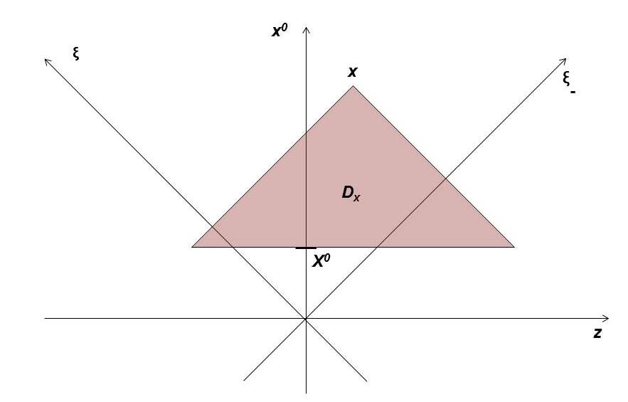
Figure 1:

In the sequel we abbreviate

$$\begin{array}[]{l}\varepsilon^{z}_{h}:=\frac{-q_{h}E^{z}}{m_{h}c^{2}},\qquad\quad Q:=\frac{2\pi}{c^{2}}\sum\limits_{h=1}^{k}\frac{q_{h}^{2}n_{h}}{m_{h}\gamma_{h}},\qquad\quad\Rightarrow\qquad\quad Q{\bm{A}}\!^{{\scriptscriptstyle\perp}}=-2\pi\sum\limits_{h=1}^{k}q_{h}n_{h}{\bm{\beta}}^{{\scriptscriptstyle\perp}}_{h};\end{array}$$ (43)

$Q$ is the sum of the squared plasma frequencies of all species of particles, divided by $2c^{2}$.

Henceforth we assume that $n_{h}(0,z)\!=\!0$ for $z\!<\!0$. Then by (12) for $x^{0}\!\leq\!0$ the EM wave is free and ${\bm{A}}\!^{{\scriptscriptstyle\perp}}$ is of the form ${\bm{A}}\!^{{\scriptscriptstyle\perp}}(x^{0},z)\equiv{\bm{\alpha}}\!^{{\scriptscriptstyle\perp}}(x^{0}\!-\!z)$, with ${\bm{\alpha}}\!^{{\scriptscriptstyle\perp}}(\xi)\!=\!0$ for $\xi\!\leq\!0$, and we may choose $X^{0}\!=\!0$ in (41) [hence $\widetilde{n_{h0}}(Z)\!\equiv\!n_{h}(0,\!Z)$]. Let $D\!_{x}\!=\!D\!_{0\!,x}$; by (41), eq. (18) equipped with such an initial condition is equivalent to the integral equation in the unknown ${\bm{A}}\!^{{\scriptscriptstyle\perp}}$

$${\bm{A}}\!^{{\scriptscriptstyle\perp}}(x^{0}\!,z)-{\bm{\alpha}}\!^{{\scriptscriptstyle\perp}}(x^{0}\!-\!z)=-\!\!\displaystyle\int_{D\!_{x}}\!\!\!\!\!\!d^{2}x^{\prime}\left[Q{\bm{A}}\!^{{\scriptscriptstyle\perp}}\right]\!\!(x^{\prime})=\!\!\displaystyle\int\limits^{x^{0}}_{0}\!\!dx^{0}{}^{\prime}\!\!\!\!\!\!\!\int\limits^{{x^{0}}\!-\!{x^{0}}^{\prime}\!+\!z}_{{x^{0}}^{\prime}\!-\!{x^{0}}\!+\!z}\!\!\!\!\!dz^{\prime}\left[2\pi\sum\limits_{h=1}^{k}q_{h}n_{h}{\bm{\beta}}^{{\scriptscriptstyle\perp}}_{h}\right]\!\!({x^{0}}^{\prime},z^{\prime});$$ (44)

Let  $s_{h}\!:=\!\gamma_{h}\!-\!u^{z}_{h}$;  this is positive-definite.  In the Lagrangian description (26) reads $\tilde{\gamma}_{h}\partial_{0}\tilde{s}_{h}=\tilde{s}_{h}\tilde{\varepsilon}^{z}_{h}\!+\!\widetilde{\partial_{-}{\bm{u}}_{h}^{{\scriptscriptstyle\perp}}{}^{2}}$; the Cauchy problem with initial condition $\tilde{s}_{h0}\!\equiv\!1$ is equivalent to the integral equation

$$\begin{array}[]{lll}\tilde{s}_{h}&:=&\tilde{\gamma}_{h}\!-\!\tilde{u}^{z}_{h}=e^{\int\limits^{x^{0}}_{0}\!\!dx^{0}{}^{\prime}\frac{\tilde{\varepsilon}^{z}_{h}}{\tilde{\gamma}_{h}}(x^{0}{}^{\prime},Z)}\!\!\!+\!\!\displaystyle\int\limits^{x^{0}}_{0}\!\!dx^{0}{}^{\prime}\,e^{\int\limits^{x^{0}}_{x^{0}{}^{\prime}}\!\!dx^{0}{}^{\prime\prime}\frac{\tilde{\varepsilon}^{z}_{h}}{\tilde{\gamma}_{h}}(x^{0}{}^{\prime\prime},Z)}\left[\frac{\widetilde{\partial_{-}{\bm{u}}_{h}^{{\scriptscriptstyle\perp}}{}^{2}}}{\tilde{\gamma}_{h}}\right]\!(x^{0}{}^{\prime},Z).\end{array}$$ (45)

It is straightforward to show that $u_{h}^{z},\gamma_{h},{\bm{\beta}}_{h}^{{\scriptscriptstyle\perp}},\beta_{h}^{z}$ are recovered from $s_{h},{\bm{u}}_{h}^{{\scriptscriptstyle\perp}}$ through the formulae

$$\begin{array}[]{ll}\displaystyle\gamma_{h}\!=\!\frac{1\!+\!{\bm{u}}_{h}^{{\scriptscriptstyle\perp}}{}^{2}\!\!+\!s_{h}^{2}}{2s_{h}},&\displaystyle{\bm{\beta}}_{h}^{{\scriptscriptstyle\perp}}\!=\!\frac{{\bm{u}}_{h}^{{\scriptscriptstyle\perp}}}{\gamma_{h}}\!=\!\frac{2s_{h}{\bm{u}}_{h}^{{\scriptscriptstyle\perp}}}{1\!+\!{\bm{u}}_{h}^{{\scriptscriptstyle\perp}2}\!\!+\!s_{h}^{2}},\\[18.0pt] \displaystyle u_{h}^{z}\!=\!\frac{1\!+\!{\bm{u}}_{h}^{{\scriptscriptstyle\perp}}{}^{2}\!\!-\!s_{h}^{2}}{2s_{h}},&\displaystyle\beta_{h}^{z}\!=\!\frac{u_{h}^{z}}{\gamma_{h}}\!=\!\frac{1\!+\!{\bm{u}}_{h}^{{\scriptscriptstyle\perp}2}\!\!-\!s_{h}^{2}}{1\!+\!{\bm{u}}_{h}^{{\scriptscriptstyle\perp}2}\!\!+\!s_{h}^{2}}.\end{array}$$ (46)

The Cauchy problem (8) with initial condition  ${\bm{x}}_{h}(0,{\bm{X}})\!=\!{\bm{X}}$  is equivalent to the integral equations

$$z_{h}(x^{0}\!,Z)=Z\!+\!\!\displaystyle\int\limits^{x^{0}}_{0}\!\!dx^{0}{}^{\prime}\,\beta_{h}^{z}[x^{0}{}^{\prime}\!,\!z_{h}(x^{0}{}^{\prime}\!,\!Z)],\qquad{\bm{x}}^{{\scriptscriptstyle\perp}}_{h}(x^{0}\!,\!{\bm{X}})={\bm{X}}^{{\scriptscriptstyle\perp}}\!+\!\!\displaystyle\int\limits^{x^{0}}_{0}\!\!dx^{0}{}^{\prime}\,{\bm{\beta}}_{h}^{{\scriptscriptstyle\perp}}[x^{0}{}^{\prime}\!,\!z_{h}(x^{0}{}^{\prime}\!,\!Z)]\qquad$$ (47)

Summing up, we have shown that making use of (15), (21), (39), (46) the determination of the evolution of the system is reduced to solving the system of integral equations (44), (45) and (47)₁ in the unknowns ${\bm{A}}\!^{{\scriptscriptstyle\perp}},s_{h},z_{h}$ [note that, once this is solved, (47)₂ becomes known].

4 Impact of a short pulse on a step-density plasma

In the present section we assume in addition that $\widetilde{n_{h0}}(Z)$ are zero for $Z\!<\!0$ and constant for $Z\!>\!0$: $\widetilde{n_{e0}}(Z)\!=\!n_{0}\theta(Z)$, etc, as depicted in fig. 2-left. Moreover, we are interested in studying the equations for so small $x^{0}$ (small times after the beginning of the interaction) that the motion of ions can be neglected. Hence we consider ions as infinitely massive, so that they remain at rest [$Z_{h}(x^{0}\!,\!z)\!\equiv\!z$ for $h\!\neq\!e$], have constant densities, and their contribution to $Q{\bm{A}}\!^{{\scriptscriptstyle\perp}}$ disappears; only electrons contribute: $Q{\bm{A}}\!^{{\scriptscriptstyle\perp}}\!=\!-2\pi en_{e}{\bm{\beta}}^{{\scriptscriptstyle\perp}}_{e}$. Choosing $\bar{Z}\!=\!0$   in (39) we find

$$E^{{\scriptscriptstyle z}}(x^{0}\!,z)=4\pi\sum\limits_{h=1}^{k}q_{h}\widetilde{N}_{h}[Z_{h}(x^{0}\!,z)]=4\pi en_{0}\left\{z\,\theta(z)\!-\!Z_{e}(x^{0}\!,z)\,\theta[Z_{e}(x^{0}\!,z)]\right\}.$$ (48)

If $z,Z\!>\!0$ this implies the well-known result (see e.g. [23, 24]) that at $x^{0}$ the electric field acting on the electrons initally located in $Z$ is  $\widetilde{E}^{{\scriptscriptstyle z}}(x^{0}\!,Z)\!=\!4\pi en_{0}\Delta z_{e}(x^{0}\!,Z)$,  i.e. proportional to the displacement  $\Delta z_{e}(x^{0}\!,Z)\!:=\!z_{e}(x^{0}\!,Z)\!-\!Z$  with respect to their initial position. The system of integral equations (44), (45), (47)₁ to be solved takes the form

$${\bm{u}}_{e}^{{\scriptscriptstyle\perp}}(x^{0}\!,z)-{\bm{u}}_{e}^{{\scriptscriptstyle\perp(0)}}(x^{0}\!-\!z)=-\frac{2\pi e^{2}}{m_{e}c^{2}}\!\!\displaystyle\int_{D\!_{x}}\!\!\!\!d^{2}x^{\prime}\>\left[n_{e}{\bm{\beta}}^{{\scriptscriptstyle\perp}}_{e}\right]\!\!(x^{\prime})$$

$$\tilde{s}_{e}=e^{\tilde{r}_{e}}\!+\!\!\displaystyle\int\limits^{x^{0}}_{0}\!\!dx^{0}{}^{\prime}\left[e^{-\tilde{r}_{e}}\frac{\widetilde{\partial_{-}{\bm{u}}_{e}^{{\scriptscriptstyle\perp}2}}}{\tilde{\gamma}_{e}}\right](x^{0}{}^{\prime}\!,Z),$$ (49)

$$\Delta z_{e}(x^{0},Z):=z_{e}(x^{0},Z)-Z=\!\!\displaystyle\int\limits^{x^{0}}_{0}\!\!dx^{0}{}^{\prime}\,\tilde{\beta}_{e}^{{\scriptscriptstyle z}}({x^{0}}^{\prime},Z)$$

($Z\geq 0$), where ${\bm{\beta}}_{e}$ is related to the unknowns ${\bm{u}}^{{\scriptscriptstyle\perp}}_{e},s_{e},z_{e}$ by (46) and, because of (21), (48)

$$n_{e}\!=\!n_{0}\,\theta[Z_{e}]\,\partial_{z}Z_{e},\qquad\tilde{r}_{e}(x^{0}\!,\!Z)\!:=\!\int\limits^{x^{0}}_{0}\!\!dx^{0}{}^{\prime}\frac{\tilde{\varepsilon}^{z}_{e}}{\tilde{\gamma}_{e}}(x^{0}{}^{\prime}\!\!,\!Z)\!=\!4K\!\!\int\limits^{x^{0}}_{Z}\!\!dx^{0}{}^{\prime}\frac{z_{e}\theta[z_{e}]\!-\!Z\theta(Z)}{\tilde{\gamma}_{e}}(x^{0}{}^{\prime}\!\!,\!Z),$$ (50)

where  $K\!:=\!\frac{\pi e^{2}n_{0}}{m_{e}c^{2}}$  ($K$ is the square of the equilibrium plasma frequency, divided by $4c^{2}$). As   $n_{e}{\bm{\beta}}^{{\scriptscriptstyle\perp}}_{e}\!\propto\!n_{e}{\bm{A}}^{{\scriptscriptstyle\perp}}\!=\!0$  outside $T$, one can replace $D\!_{x}$ by $D\!_{x}\cap T$ in (49)₁.

For $n_{0}\!=\!0$ the solution of (49) is $({\bm{u}}^{{\scriptscriptstyle\perp}}_{e},\tilde{s}_{e},z_{e})=({\bm{u}}^{{\scriptscriptstyle\perp(0)}}_{e},1,z_{e}^{{\scriptscriptstyle(0)}})$. For $n_{0}\!>\!0$ we can approximate better and better the solution by an iterative procedure: replacing the approximation after $k$ steps [which we will distinguish by the superscript $(k)$] at the rhs of (49) we will obtain at the left-hand side (lhs) the approximation after $k\!+\!1$ steps [5]. Here we stick to the first step ($k\!=\!0$),

$${\bm{u}}_{e}^{{\scriptscriptstyle\perp(1)}}(x^{0}\!,z)-{\bm{u}}_{e}^{{\scriptscriptstyle\perp(0)}}(x^{0}\!-\!z)=-\frac{2\pi e^{2}}{m_{e}c^{2}}\!\!\displaystyle\int_{D\!_{x}}\!\!\!\!d^{2}x^{\prime}\>\left[n_{e}^{{\scriptscriptstyle(0)}}{\bm{\beta}}^{{\scriptscriptstyle\perp(0)}}_{e}\right]\!\!(x^{\prime})$$

$$\tilde{s}_{e}^{{\scriptscriptstyle(1)}}=e^{\tilde{r}_{e}^{{\scriptscriptstyle(0)}}}\!+\!\!\displaystyle\int\limits^{x^{0}}_{0}\!\!dx^{0}{}^{\prime}\,\left[e^{-\tilde{r}_{e}^{{\scriptscriptstyle(0)}}}\frac{\widetilde{\partial_{-}{\bm{u}}_{e}^{{\scriptscriptstyle\perp(0)}2}}}{\tilde{\gamma}_{e}^{{\scriptscriptstyle(0)}}}\right]\!(x^{0}{}^{\prime}\!,Z)=e^{\tilde{r}_{e}^{{\scriptscriptstyle(0)}}},$$ (51)

$$\Delta z_{e}^{{\scriptscriptstyle(1)}}(x^{0},Z):=z_{e}^{{\scriptscriptstyle(1)}}(x^{0},Z)-Z=\!\!\displaystyle\int\limits^{x^{0}}_{0}\!\!dx^{0}{}^{\prime}\,\tilde{\beta}_{e}^{{\scriptscriptstyle z(1)}}({x^{0}}^{\prime},Z),$$

and investigate for how long $({\bm{u}}^{{\scriptscriptstyle\perp(1)}}_{e},\tilde{s}^{{\scriptscriptstyle\perp(1)}}_{e},z_{e}^{{\scriptscriptstyle(1)}})$ remains “close” to $({\bm{u}}^{{\scriptscriptstyle\perp(0)}}_{e},1,z_{e}^{{\scriptscriptstyle(0)}})$. In (51) the tilde is to be understood as the change from the Eulerian to the Lagrangian description performed approximating ${\bm{x}}_{e}$ by ${\bm{x}}_{e}^{{\scriptscriptstyle(0)}}$, and in the second line we have used $\partial\!_{{\scriptscriptstyle-}}{\bm{u}}_{e}^{{\scriptscriptstyle\perp(0)}2}\!=\!0$. The electron density obtained approximating $z_{e}$ by $z_{e}^{{\scriptscriptstyle(0)}}$, i.e. replacing (30) in (50)₁ or equivalently $\widetilde{n_{e0}}(Z)\!=\!n_{0}\theta(Z)$ in (37), is

$$n_{e}^{{\scriptscriptstyle(0)}}(x^{0}\!,z)=n_{0}\,\theta\left[z\!-\!Y^{3}_{e}(x^{0}\!-\!z)\right]\,\gamma_{e}^{{\scriptscriptstyle(0)}}(x^{0}\!-\!z).$$ (52)

In the appendix we prove that for $Z\geq 0$ we can give $\tilde{r}_{e}^{{\scriptscriptstyle(0)}}$ the more explicit form

$$\tilde{r}_{e}^{{\scriptscriptstyle(0)}}(x^{0}\!,Z)\,=\,4K\,V_{e}^{3}\!\left[\Xi_{e}^{-1}\!(x^{0}\!\!-\!Z)\right],\qquad\qquad\mbox{where }\quad V_{e}^{3}(\xi):=\displaystyle\int^{\xi}_{0}\!\!dy\,Y^{3}_{e}(y).$$ (53)

As $Y^{3}_{e}(\xi)$ is strictly increasing, $V_{e}^{3}(\xi),r_{e}^{{\scriptscriptstyle(0)}}(\xi)$ are not only strictly increasing, but also convex in all $]0,l[$. This implies $V_{e}^{3}(\xi)/Y_{e}^{3}(\xi)\!<\!\xi/2$ at least.

Now assume that ${\bm{E}}^{{\scriptscriptstyle\perp}}(x^{0}\!,z)\!=\!{\bm{\epsilon}}^{{\scriptscriptstyle\perp}}(x^{0}\!-\!z)$ with ${\bm{\epsilon}}^{{\scriptscriptstyle\perp}}(\xi)\!=\!\epsilon_{s}(\xi){\bm{\epsilon}}_{o}^{{\scriptscriptstyle\perp}}(\xi)$, where the envelope amplitude $\epsilon_{s}(\xi)\!\geq\!0$ has a finite support $[0,l]$  (as depicted in fig. 2-left) and slowly varies on the scale $\lambda\!\ll\!l$, and ${\bm{\epsilon}}_{o}^{{\scriptscriptstyle\perp}}(\xi)$ is a sinusoidally oscillating transverse vector with period $\lambda\!:=\!2\pi/k$. For the sake of definiteness, we shall consider

$$\begin{array}[]{lll}{\bm{\epsilon}}_{o}^{{\scriptscriptstyle\perp}}(\xi)\!=\!{\hat{\bm{x}}}\cos k\xi,&{\bm{\epsilon}}_{p}^{{\scriptscriptstyle\perp}}(\xi)\!=\!{\hat{\bm{x}}}\sin k\xi&\mbox{(linear polarization), or}\\[8.0pt] {\bm{\epsilon}}_{o}^{{\scriptscriptstyle\perp}}(\xi)\!=\!{\hat{\bm{x}}}\cos k\xi\!+\!{\hat{\bm{y}}}\sin k\xi,&{\bm{\epsilon}}_{p}^{{\scriptscriptstyle\perp}}(\xi)\!=\!{\hat{\bm{x}}}\sin k\xi\!-\!{\hat{\bm{y}}}\cos k\xi&\mbox{(circular polarization).}\end{array}$$ (54)

Then  ${\bm{\alpha}}^{{\scriptscriptstyle\perp}}(\xi)\!\simeq\!\frac{1}{k}\epsilon_{s}{\bm{\epsilon}}_{p}^{{\scriptscriptstyle\perp}}(\xi)$,  and, setting  $w\!:=\!\frac{e}{kmc^{2}}\epsilon_{s}$,  ${\bm{u}}_{e}^{{\scriptscriptstyle\perp(0)}}(\xi)\!\simeq\!w(\xi){\bm{\epsilon}}_{p}^{{\scriptscriptstyle\perp}}(\xi)$,  ${\bm{Y}}_{e}\!^{{\scriptscriptstyle\perp}}\!(\xi)\!\simeq\!-\frac{1}{k}w(\xi){\bm{\epsilon}}_{o}^{{\scriptscriptstyle\perp}}(\xi)$,   $u_{e}^{{\scriptscriptstyle z(0)}}(\xi)\!\simeq\!\frac{1}{2}w^{2}(\xi){\bm{\epsilon}}_{p}^{{\scriptscriptstyle\perp 2}}(\xi)$.  Denoting the first (possibly unique) maximum point of  ${\bm{\alpha}}^{{\scriptscriptstyle\perp}2}$  as  $\xi_{0}$,  in the appendix we give the rhs(51)₁ the more explicit expression (79) and prove for  $0\!\leq\!\xi\!\leq\!\xi_{0}$ and either polarization the inequality

$$\frac{|{\bm{A}}^{{\scriptscriptstyle\perp(1)}}(\xi,\xi_{{\scriptscriptstyle-}})\!-\!{\bm{\alpha}}^{{\scriptscriptstyle\perp}}(\xi)|}{\epsilon_{s}(\xi)/k}=\frac{|{\bm{u}}_{e}^{{\scriptscriptstyle\perp(1)}}(\xi,\xi_{{\scriptscriptstyle-}})\!-\!{\bm{u}}_{e}^{{\scriptscriptstyle\perp(0)}}(\xi)|}{w(\xi)}\leq\frac{K\lambda\xi_{{\scriptscriptstyle-}}}{2\pi}.$$ (55)

The lhs is the difference between ${\bm{u}}_{e}^{{\scriptscriptstyle\perp(1)}},{\bm{u}}_{e}^{{\scriptscriptstyle\perp(0)}}$ (or, equivalently, the difference between ${\bm{A}}^{{\scriptscriptstyle\perp(1)}},{\bm{\alpha}}^{{\scriptscriptstyle\perp}}$) normalized by their modulating envelope amplitude; if the polarization is circular then $|{\bm{\epsilon}}_{p}^{{\scriptscriptstyle\perp}}|\!=\!1$, and the lhs is exactly the modulus of the relative difference between ${\bm{u}}_{e}^{{\scriptscriptstyle\perp(1)}},{\bm{u}}_{e}^{{\scriptscriptstyle\perp(0)}}$ (or, equivalently, ${\bm{A}}^{{\scriptscriptstyle\perp(1)}},{\bm{\alpha}}^{{\scriptscriptstyle\perp}}$). If $\xi_{{\scriptscriptstyle-}}\!\ll\!\frac{2\pi}{K\lambda}$ then lhs$\leq$rhs$\ll\!1$. So we can approximate

$${\bm{u}}_{e}^{{\scriptscriptstyle\perp}}\!\simeq\!{\bm{u}}_{e}^{{\scriptscriptstyle\perp(1)}}\!\simeq\!{\bm{u}}_{e}^{{\scriptscriptstyle\perp(0)}}\qquad\quad\mbox{in the space-time region }\>\>0\!\leq\!\xi\!\leq\!\xi_{0},\quad 0\!\leq\!\xi_{{\scriptscriptstyle-}}\!\ll\!\frac{2\pi}{K\lambda}.$$ (56)

Consequently and by (46), in the region (56) we find by some computation

$$\beta_{e}^{{\scriptscriptstyle z(1)}}\!=\!\frac{1\!+\!{\bm{u}}_{e}^{{\scriptscriptstyle\perp(1)}2}\!\!-\!s^{{\scriptscriptstyle(1)}2}_{e}}{1\!+\!{\bm{u}}_{e}^{{\scriptscriptstyle\perp(1)}2}\!\!+\!s^{{\scriptscriptstyle(1)}2}_{e}}\!\simeq\!\frac{1\!+\!{\bm{u}}_{e}^{{\scriptscriptstyle\perp(0)}2}\!\!-\!e^{2r^{{\scriptscriptstyle(0)}}_{e}}}{1\!+\!{\bm{u}}_{e}^{{\scriptscriptstyle\perp(0)}2}\!\!+\!e^{2r^{{\scriptscriptstyle(0)}}_{e}}}=\frac{2(1\!+\!2u_{e}^{{\scriptscriptstyle z(0)}})}{1\!+\!2u_{e}^{{\scriptscriptstyle z(0)}}\!\!+\!e^{2r^{{\scriptscriptstyle(0)}}_{e}}}\!-\!1,\qquad$$ (57)

$$\Delta z_{e}^{{\scriptscriptstyle(1)}}(x^{0}\!,\!Z)=\!\displaystyle\int\limits^{x^{0}}_{Z}\!\!dx^{0}{}^{\prime}\,\tilde{\beta}_{e}^{{\scriptscriptstyle z(1)}}(x^{0}{}^{\prime}\!\!,\!Z)\simeq\!\!\!\!\!\!\!\displaystyle\int\limits^{\Xi_{e}^{-1}\!(x^{0}\!\!-\!Z)}_{0}\!\!\!\!\!\!\!\!dy\,[\gamma_{e}^{{\scriptscriptstyle(0)}}\beta_{e}^{{\scriptscriptstyle z(1)}}](y),\qquad$$ (58)

$$0\leq[z_{e}^{{\scriptscriptstyle(0)}}\!-\!z_{e}^{{\scriptscriptstyle(1)}}](x^{0}\!,\!Z)\simeq G[\Xi_{e}^{-1}\!(x^{0}\!\!-\!Z)],\qquad G(\xi)\!:=\!\!\int\limits^{\xi}_{0}\!\!\!dy\,g(y),\quad g:=\frac{\left(\!1\!+\!2u_{e}^{{\scriptscriptstyle z(0)}}\!\right)\!\left(\!e^{2r^{{\scriptscriptstyle(0)}}_{e}}\!\!\!-\!1\!\!\right)}{1\!+\!2u_{e}^{{\scriptscriptstyle z(0)}}\!+\!e^{2r^{{\scriptscriptstyle(0)}}_{e}}},\qquad$$ (59)

$$0\leq\frac{\Delta z_{e}^{{\scriptscriptstyle(0)}}\!-\!\Delta z_{e}^{{\scriptscriptstyle(1)}}}{\Delta z_{e}^{{\scriptscriptstyle(0)}}}(x^{0}\!,\!Z)=\frac{z_{e}^{{\scriptscriptstyle(0)}}(x^{0}\!,\!Z)\!-\!z_{e}^{{\scriptscriptstyle(1)}}(x^{0}\!,\!Z)}{z_{e}^{{\scriptscriptstyle(0)}}(x^{0}\!,\!Z)\!-\!Z}\simeq T[\Xi_{e}^{-1}\!(x^{0}\!\!-\!Z)],\qquad\qquad T\!:=\!\frac{G}{Y_{e}^{3}}.\qquad$$ (60)

By (60), $T[\Xi_{e}^{-1}\!(x^{0}\!\!-\!Z)]$ gives the relative difference between the displacement $\Delta z_{e}$ in the zero-density and in the first corrected approximation. Hence the approximation  $z_{e}(x^{0}\!,\!Z)\!\simeq\!z_{e}^{{\scriptscriptstyle(1)}}(x^{0}\!,\!Z)\!\simeq\!z_{e}^{{\scriptscriptstyle(0)}}(x^{0}\!,\!Z)$ may be good only as long as  $T[\Xi_{e}^{-1}\!(x^{0}\!\!-\!Z)]\!\ll\!1$. By (35), the maximum ${\bm{\alpha}}^{{\scriptscriptstyle\perp}}(\xi_{0})$ reaches the electrons initially located in $Z$ at the time $\bar{x}^{0}(Z)\!=\!\Xi_{e}(\xi_{0})\!+\!Z$; therefore the approximation  $z_{e}(x^{0}\!,\!Z)\!\simeq z_{e}^{{\scriptscriptstyle(0)}}(x^{0}\!,\!Z)$ may be good for all $x^{0}\!\leq\!\bar{x}^{0}(Z)$ if

$$T(\xi)\ll 1\qquad\quad 0\leq\xi\leq\xi_{0},\qquad\qquad\qquad 2Y^{3}_{e}(\xi_{0})\!+\!\xi_{0}\!+\!2Z\ll\frac{2\pi}{K\lambda}.$$ (61)

The condition at the right guarantees that (56) is fulfilled, since $\bar{x}^{0}\!+\!z_{e}^{{\scriptscriptstyle(0)}}(\bar{x}^{0}\!,Z)\!=\!2Y^{3}_{e}(\xi_{0})\!+\!\xi_{0}\!+\!2Z$. In $[0,\xi_{0}]$ $g(\xi)$ is strictly increasing , hence $G(\xi)$ is strictly increasing and convex. Moreover, as $\xi\!\to\!0$ $g(\xi)\!\simeq\!2r^{{\scriptscriptstyle(0)}}_{e}(\xi)$, whence $G(\xi)\!<\!g(\xi)\xi/2\!\lesssim\!4K\xi V^{3}_{e}(\xi)\!<2K\xi^{2}Y^{3}_{e}(\xi)$ at least, and we find not only $g(0)\!=\!G(0)\!=\!0$, but also $T(0)\!=\!0$, as expected. In fig. 3 we plot $T(\xi)$ for a gaussian pulse and several values of $K$; it is a strictly increasing, convex function.

If (61) is fulfilled then by (36) the displacement at time $\bar{x}^{0}$ of the electrons initially located at $Z=Z$ is independent of $Z$ and approximately equal to

$$\zeta(Z)\simeq Y^{3}_{e}(\xi_{0})=\frac{1}{2}\xi_{0}u_{e\,m}^{{\scriptscriptstyle\perp}2}=\!\!\int\limits^{\xi_{0}}_{0}\!\!\!d\xi\,u_{e}^{{\scriptscriptstyle z(0)}}(\xi)=\!\!\int\limits^{\xi_{0}}_{0}\!\!\!d\xi\,\frac{p}{2}w^{2}\!(\xi),\qquad p\!=\!\left\{\!\!\begin{array}[]{ll}1&\mbox{circ. pol.}\\ \frac{1}{2}&\mbox{lin. pol.};\end{array}\right.$$ (62)

here $p\!\simeq\!1/2$ for linear polarization comes from the mean of  $\sin^{2}\!k\xi$   over a period   $\lambda$,   and $u_{e\,m}^{{\scriptscriptstyle\perp}2}$ stands for the mean of ${\bm{u}}_{e}^{{\scriptscriptstyle\perp}2}$ over $[0,\xi_{0}]$ (if $w$ is symmetric around a unique maximum at $\xi_{0}=l/2$, the latter coincides with the mean over all $[0,l]$).

By (57), the monotonicity of $r_{e}^{{\scriptscriptstyle(0)}}$ and the fact that  $u_{e}^{{\scriptscriptstyle z(0)}}(\xi)\!\propto\!w^{2}(\xi)\!\to\!0$  as  $\xi\!\to\!l$, there exists (at least) a point in $]\xi_{0},l]$ where $\beta_{e}^{{\scriptscriptstyle z(1)}}$ vanishes; let $\xi_{1}$ be the first one. Namely, in the first corrected approximation the electrons at some point invert their motion, as we expect due to the restoring electric back-force exerted by the ions. The condition $\beta_{e}^{{\scriptscriptstyle z(1)}}(\xi_{1})\!=\!0$ amounts to $1\!+\!2u_{e}^{{\scriptscriptstyle z(0)}}\!(\xi_{1})=\exp[8KV_{e}^{3}(\xi_{1})]$. Fixing $\xi_{1}$, this can be solved for $K$ (which is physically tunable by the choice of $n_{0}$):

$$K\equiv K(\xi_{1})=\frac{\ln[1\!+\!2u_{e}^{{\scriptscriptstyle z(0)}}\!(\xi_{1})]}{8V_{e}^{3}(\xi_{1})}=\frac{\ln[1\!+\!pw^{2}\!(\xi_{1})]}{8V_{e}^{3}(\xi_{1})};$$ (63)

Manifestly, $K(\xi_{1})$ is a strictly decreasing function from $K(0)\!=\!\infty$ to $K(l)\!=\!0$.  The displacement (62) will be approximately the maximal one if $0\!<\!(\xi_{1}\!-\!\xi_{0})/\xi_{0}\!\ll\!1$, while (61) is respected. To check these conditions one can proceed by “trial and error”: choosing $\xi_{1}$ close to $\xi_{0}$, computing $K$ and checking whether (61) is fulfilled. If so, (62) is reliable for that value, and all smaller values, of $K$. If not, one has to try with a larger $\xi_{1}$, which will give a smaller $K$ and a smaller $T(\xi)$ for $\xi\!\in\![0,\xi_{0}]$, until the maximum $T(\xi)$ [tipically, $T(\xi_{0})$] is small enough.

4.1 The slingshot effect

The basic formula (62) for the displacement is used in [1] to predict and estimate the slingshot effect, i.e. the expulsion in the negative $z$-direction of the plasma eletrons initially located around $Z\!=\!0$, shortly after the impact of a suitable ultra-short and ultra-intense laser pulse in the form of a pancake normally onto a plasma. The mechanism is very simple: the plasma electrons in a thin layer - just beyond the surface of the plasma - first are given sufficient electric potential energy by the displacement (62) with respect to the ions, then after the pulse are pulled back by the longitudinal electric force exerted by the latter and may leave the plasma. Sufficient conditions for this to happen are that the pancake is sufficiently thin ($R\!\gg l$), its radius $R$ is not too small ($R\!\gtrsim\!\zeta$), the EM field inside is sufficiently intense, and the electron density $n_{0}$ is sufficiently low. $R\!\gg l$ guarantees that the plane wave solutions considered in the previous sections are sufficiently accurate in the plasma, especially in the forward boost phase, in the internal part of a cylinder of radius $R$. $R\!\gtrsim\!\zeta$ avoids that the way out of the mentioned thin layer of electrons within such a cylinder is blocked by the electrons initially located just outside the cylindrical surface (which are attracted and move towards the cylinder axis). The high intensity of the EM field and the sufficiently low plasma density are needed for the longitudinal electric force to induce the back-acceleration of the electrons after the pulse maximum has overcome them, in phase with the negative ponderomotive force exerted by the pulse in its decreasing stage. Actually we impose the stronger condition that $n_{0}$ is sufficiently low in order that (61) is fulfilled, and the estimate (62) of the displacement at lowest order is reliable. As a result, the final energy of the electrons initially located at $Z\!=\!0$ after the expulsion is [1]

$${}H=m{}c^{2}\gamma_{e{\scriptscriptstyle M}},\qquad\qquad\gamma_{e{\scriptscriptstyle M}}\simeq 1+2K\zeta^{2}.$$ (64)

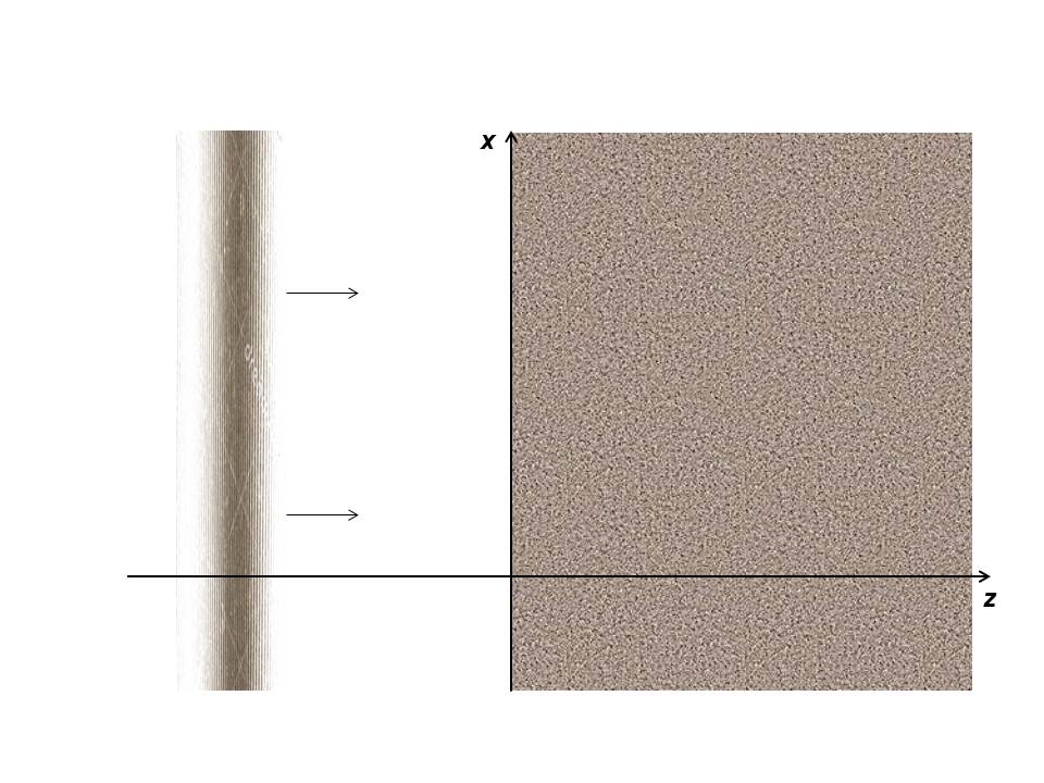
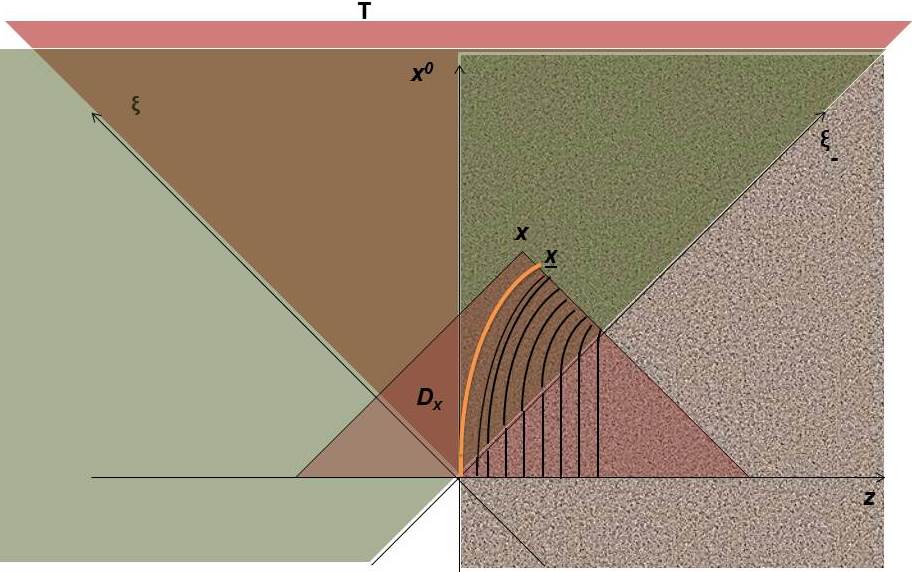
Figure 2:

The EM energy carried by the pulse within the pancake cylinder $V$ of radius $R$ is

$${\cal E}=\!\int_{V}\!\!dV\,\frac{{\bm{E}}^{{\scriptscriptstyle\perp}2}\!\!+\!{\bm{B}}^{{\scriptscriptstyle\perp}2}}{8\pi}\!\simeq\!\frac{R^{2}}{4}\!\!\int_{0}^{l}\!\!\!\!d\xi\,{\bm{E}}^{{\scriptscriptstyle\perp}2}\!\simeq\!\frac{(\pi R)^{2}}{\lambda^{2}}\!\!\int_{0}^{l}\!\!\!\!d\xi\,{\bm{A}}^{{\scriptscriptstyle\perp}2}\!\simeq\!\frac{(mc^{2}\!\pi R)^{2}}{(e\lambda)^{2}}\!\!\int_{0}^{l}\!\!\!\!d\xi\,pw^{2}\!=\!\frac{2(mc^{2}\!\pi R)^{2}}{(e\lambda)^{2}}Y_{e}^{3}(l)$$ (65)

Assuming for simplicity that the modulating amplitude $w$ is symmetric around $\xi_{0}\!=\!l/2$, it follows $Y_{e}^{3}(l)=2Y_{e}^{3}(\xi_{0})$. Requiring $R\!=\!\nu\zeta$ (with some number  $\nu\!\sim\!1$)   we find by (62)

$${}\nu\zeta\!=\!R\!=\!\left[\!\frac{\nu{\cal E}(e\lambda)^{2}}{4(\pi m{}c^{2})^{2}}\!\right]^{\frac{1}{3}}.$$ (66)

We consider two prototype modulating amplitudes with a unique maximum in $\xi_{0}=l/2$, and symmetric with respect to $\xi_{0}$, namely a gaussian and a fourth degree polynomial with the same maximum point $\xi_{0}$, multiplied by the characteristic functions resp. of $[0,l]$ and of $\left[\frac{l-l_{p}}{2},\frac{l+l_{p}}{2}\right]$  (with $l_{p}\!\leq\!l$ the length of the support of $w_{p}$):

$$\begin{array}[]{l}w_{g}(\xi)\!=\!a_{g}\,\exp\!\left[-\frac{(\xi\!-\!\xi_{0})^{2}}{2\sigma}\right]\theta\!\left[\!\frac{1}{4}\!-\!\left(\!\frac{\xi}{l}\!-\!\frac{1}{2}\!\right)^{2}\right]\!,\qquad w_{p}(\xi)\!=\!a_{p}\,\left[\!\frac{1}{4}\!-\!\left(\!\frac{\xi-\xi_{0}}{l_{p}}\right)^{2}\!\right]^{2}\theta\!\left[\!\frac{1}{4}\!-\!\left(\!\frac{\xi-\xi_{0}}{l_{p}}\right)^{2}\!\right].\end{array}$$ (68)

Let $l^{\prime}_{g},l^{\prime}_{p}$ be the widths at half height of $w_{g}^{2},w_{p}^{2}$. We adjust the parameters $a_{p},a_{g},l_{p},\sigma$ so that $l^{\prime}_{g}\!=\!l^{\prime}_{p}$ and the pulses corresponding to $w_{g},w_{p}$ have the same energy (65), i.e. $\int_{-\infty}^{\infty}\!d\xi\,w_{p}^{2}=\int_{-\infty}^{\infty}\!d\xi\,w_{g}^{2}$; we assume $l$ large enough (say $l\geq 3\sqrt{\sigma}$ ) for the integral of $w^{2}_{g}$ to be practically equal to its value for $l\!=\!\infty$. By straightforward computations in the appendix we show that these two conditions amount to:

$$2Y_{e}^{3}\!(\xi_{0})=Y_{e}^{3}(l)=\frac{p}{1260}a_{p}^{2}l_{p}\simeq\frac{p}{2}a_{g}^{2}\sqrt{\pi\sigma},\qquad\qquad 0.4l_{p}\!\simeq\!l^{\prime}_{p}\!=\!l^{\prime}_{g}\!=\!2\sqrt{\sigma\ln 2}.$$ (69)

Consequently, and by (65-66),

$$Y_{e}^{3}\!(\xi_{0})\!=\!\zeta\!=\!\left[\!\frac{{\cal E}(e\lambda)^{2}}{4(\nu\pi m{}c^{2})^{2}}\!\right]^{\frac{1}{3}}\qquad\quad\begin{array}[]{ll}\sigma\!=\!\frac{l^{\prime}_{g}{}^{2}}{4\ln 2},&a_{g}^{2}\!=\!\frac{4}{p\sqrt{\pi\sigma}}Y_{e}^{3}\!(\xi_{0})\!=\!\frac{8\sqrt{\ln 2}}{p\sqrt{\pi}l^{\prime}_{g}}\left[\!\frac{{\cal E}(e\lambda)^{2}}{4(\nu\pi m{}c^{2})^{2}}\!\right]^{\frac{1}{3}},\\[10.0pt] l_{p}\!\simeq\!\frac{5l^{\prime}_{g}}{2},&a_{p}^{2}\!=\!\frac{1008}{pl_{g}^{\prime}}Y_{e}^{3}\!(\xi_{0})\!=\!\frac{1008}{pl_{g}^{\prime}}\left[\!\frac{{\cal E}(e\lambda)^{2}}{4(\nu\pi m{}c^{2})^{2}}\!\right]^{\frac{1}{3}}.\end{array}$$ (70)

The laser machine at the Flame facility in Frascati can shoot [26, 27] linearly polarized pulses  ($p\!=\!1/2$)  with  $\lambda\!\simeq\!8\!\times\!10^{-5}cm$,  energy  ${\cal E}\!=\!5\!\times\!10^{7}erg$,  an approximately gaussian longitudinal modulating amplitude with width at half height  $l^{\prime}\!\simeq\!7.5\!\times\!10^{-4}cm$,  and a radius $R$ which can be tuned by focalization in the range  $10^{-4}\div 1\,cm$ .  Imposing $l^{\prime}_{g}\!=\!l^{\prime}_{p}\!=\!l^{\prime}$, these data and formulae (65-70) respectively yield for  $\nu\!=\!1,2$

$$\nu\!=\!1:\qquad\quad Y_{e}^{3}\!(\xi_{0})\!=\!\zeta\!=\!1.4\!\times\!10^{-3}cm,\qquad\begin{array}[]{ll}\displaystyle\sigma\!\simeq\!2\!\times\!10^{-7}cm^{2},&\displaystyle a_{g}\!\simeq\!3.75,\\[10.0pt] \displaystyle l_{p}\!\simeq\!1.875\!\times\!10^{-3}cm,&\displaystyle a_{p}\!\simeq\!61.5.\end{array}\qquad\quad$$ (73)

$$\nu\!=\!2:\qquad\quad Y_{e}^{3}\!(\xi_{0})\!=\!\zeta\!\simeq\!8.8\!\times\!10^{-4}cm,\qquad\begin{array}[]{ll}\displaystyle\sigma\!\simeq\!2\!\times\!10^{-7}cm^{2},&\displaystyle a_{g}\!\simeq\!2.98,\\[10.0pt] \displaystyle l_{p}\!\simeq\!1.875\!\times\!10^{-3}cm,&\displaystyle a_{p}\!\simeq\!48.8.\end{array}\qquad\quad$$ (76)

A plasma with $n_{0}\!\geq\!10^{17}cm^{-3}$ is obtained by ionization from an ultracold gas (typically, helium) jet in a vacuum chamber hit by such an energetic laser pulse as soon as $\Gamma_{i}\!<\!1$. Here $\Gamma_{i}\!:=\!\sqrt{U_{i}/\kappa}\!=\!\sqrt{2U_{i}/m{}c^{2}u_{e{\scriptscriptstyle}}^{{\scriptscriptstyle\perp}2}}\!\simeq\!\sqrt{2U_{i}/m{}c^{2}pw^{2}(\xi)}$ ($\kappa\!\equiv$kinetic energy) are the Keldysh parameters (the ionization potentials $U_{i}$ are about $24eV,\,54eV$ for first and second ionization respectively). We define the $l$ of (68) as the length of the $z$-interval where the Keldysh parameter of first ionization corresponding to the gaussian pulse fulfills $\Gamma_{i}\leq 1$; from $1\!=\!\Gamma_{i}^{2}\!=\!4U_{i}/m{}c^{2}w_{g}^{2}(0)\!=\!4U_{i}/m{}c^{2}a_{g}^{2}\exp[-l^{2}/4\sigma]$  we find  for either value of $\nu$ $l\!\simeq\!3\!\times\!10^{-3}cm$,   whence $\xi_{0}\!\simeq\!1.5\!\times\!10^{-3}cm$. The ionization is practically complete and immediate [25, 26] because the Keldysh parameter for double ionization reaches values $\Gamma_{i}\!<\!1/100$ very fast.

In the case $\nu\!=\!1$, choosing e.g.  $\xi_{1}\!-\!\xi_{0}\!=\!l_{p}/20\simeq l^{\prime}_{g}/8\simeq 0.06\xi_{0}$  and computing (63) numerically (we have used the software Mathematica), one finds  $4l^{\prime}_{g}{}^{2}K_{g}(\xi_{1})\!\simeq\!\xi_{0}^{2}K_{g}(\xi_{1})\simeq 2$,  $4l^{\prime}_{p}{}^{2}K_{p}(\xi_{1})\!\simeq\!\xi_{0}^{2}K_{p}(\xi_{1})\!\simeq\!2.2$,  which by (55)corresponds to  $n_{0}\!\simeq\!1\div 1.1\times 10^{18}cm^{-3}$.

In fig. 3 we plot $w_{g}(\xi)$ (blue line) and $w_{p}(\xi)$ (purple line) together with the corresponding $u_{e}^{{\scriptscriptstyle z(0)}},Y^{3}_{e},V^{3}_{e},\beta_{e}^{{\scriptscriptstyle z(1)}},g,G,T$ for circular polarization ($p\!=\!1$) and $\nu\!=\!1$, $a_{g}=3.75$, $a_{p}=61.5$, $2\xi_{0}\!=\!l\!=\!3\!\times\!10^{-3}cm$, $K\xi_{0}^{2}\!=\!2$. As manifest from these plots, the polynomial and the gaussian modulating amplitude with the same energy and width at half height do not lead to significant differences. As one can see from comparison of the graphs, the tiny tail of the gaussian outside the support of $w_{p}$ has a not completely negligible effects, because it leads to a relative error $T_{g}(\xi_{0})\!\simeq\!0.2$ instead of $T_{p}(\xi_{0})\!\simeq\!0.16$. However, as both $T_{g}(\xi_{0}),T_{p}(\xi_{0})\!\ll\!1$ we can consider (61) with such a $K$ fulfilled and the above calculations leading to (62) reliable. By (64), this leads to the slingshot effect with expulsion of the surface electrons with a final energy $H\!\simeq\!2.3\,MeV$.

In the case $\nu\!=\!2$, choosing  $\xi_{1}\!-\!\xi_{0}\!\simeq\!0.19l^{\prime}_{g}\simeq 0.094\xi_{0}$  and computing (63) numerically, one finds  $l^{\prime}_{g}{}^{2}K_{g}(\xi_{1})\!\simeq\!0.32$,  which by (55) corresponds to  $n_{0}\!\simeq\!7\times 10^{17}cm^{-3}$. This leads to relative errors $T_{g}(\xi_{0})\!\simeq\!0.22$, $T_{p}(\xi_{0})\!\simeq\!0.18$. Again, as both $T_{g}(\xi_{0}),T_{p}(\xi_{0})\!\ll\!1$ we can consider (61) with such a $K$ fulfilled and the above calculations leading to (62) reliable. By (64), this leads to the slingshot effect with expulsion of the surface electrons with a final energy $H\!\simeq\!0.96\,MeV$.

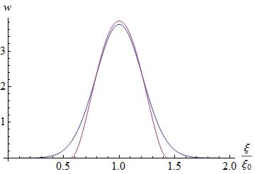
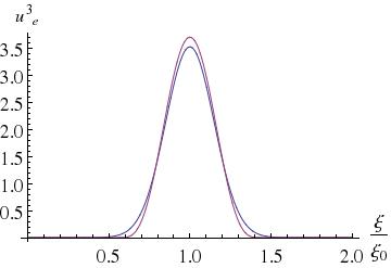
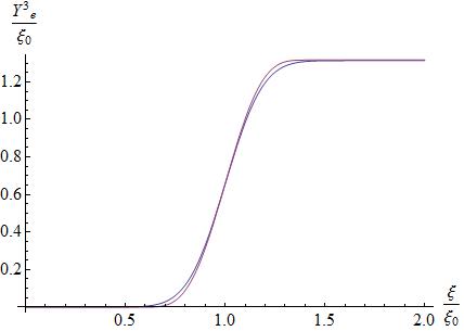
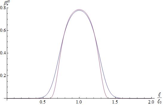
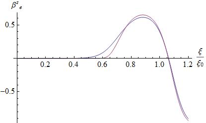
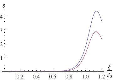
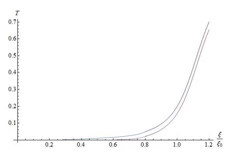
Figure 3: The graphs of $w,u_{e}^{{\scriptscriptstyle z(0)}},Y^{3}_{e},V^{3}_{e},\beta_{e}^{{\scriptscriptstyle z(0)}},\beta_{e}^{{\scriptscriptstyle z(1)}},g,T$ for $w(\xi)\!=\!w_{g}(\xi)$ (blue curve) and $w(\xi)\!=\!w_{p}(\xi)$ (purple curve) and $K\xi_{0}^{2}\!=\!2$, corresponding to $n_{0}\!\simeq\!10^{18}cm^{-3}$.  In either case $T(\xi)$ is manifestly strictly increasing, and $T(\xi_{0})\!\ll\!1$.

Acknowledgments.   It is a pleasure to thank R. Fedele and U. De Angelis for stimulating discussions and constant encouragement. I also acknowledge useful suggestions on the use of Mathematica by S. De Nicola.

5 Appendix

5.1  Proof of (53).   We use (50), (29), the inequality  $z_{e}^{{\scriptscriptstyle(0)}}(x^{0}\!\!,\!Z)\!>\!0$  for all  $x^{0}\!>\!Z$,  change integration variable  $s\!\mapsto\!y\!:=\!s\!-\!z_{e}^{{\scriptscriptstyle(0)}}(s\!,\!Z)\!=\!\Xi_{e}^{-1}\!(s\!-\!Z)$  and abbreviate  $\hat{\xi}(x^{0}\!,\!Z)\!:=\!\Xi_{e}^{-1}\!(x^{0}\!\!-\!Z)$:

$$\begin{array}[]{l}\frac{\tilde{r}_{e}^{{\scriptscriptstyle(0)}}\!(x^{0}\!,Z)}{4K}\!=\!\!\int\limits^{x^{0}}_{Z}\!\!ds\frac{z_{e}^{{\scriptscriptstyle(0)}}\theta[z_{e}^{{\scriptscriptstyle(0)}}]\!-\!Z}{\tilde{\gamma}_{e}^{{\scriptscriptstyle(0)}}}(s\!,\!Z)\!=\!\int\limits^{x^{0}}_{Z}\!\!ds\frac{z_{e}^{{\scriptscriptstyle(0)}}\!(s\!,Z)\!-\!Z}{\gamma_{e}^{{\scriptscriptstyle(0)}}\![s\!-\!z_{e}^{{\scriptscriptstyle(0)}}\!(s\!,Z)]}\!=\!\int\limits^{x^{0}}_{Z}\!\!ds\frac{s\!-\!Z\!-\!\Xi_{e}^{-1}\!(s\!-\!Z)}{\gamma_{e}^{{\scriptscriptstyle(0)}}[\Xi_{e}^{-1}\!(s\!-\!Z)]}=\!\!\int\limits^{\hat{\xi}}_{0}\!\!dy\,[\Xi_{e}\!(y)\!-\!y]\!=\!\!\int\limits^{\hat{\xi}}_{0}\!\!dy\,Y^{3}_{e}\!(y)=V_{e}^{3}\!\!\left[\hat{\xi}\right].\end{array}$$

5.2  A more explicit expression and a upper bound for the rhs(51)₁.    Let $\underline{x}(\xi_{{\scriptscriptstyle-}})$ be the intersection (see fig. 2 -right) in the $(x^{0},z)$ plane of the trajectory $(x^{0},z_{e}^{{\scriptscriptstyle(0)}}(x^{0}\!,0))$ (plot in light orange) with the line of equation  $x^{0}\!+\!z=\xi_{{\scriptscriptstyle-}}$,  $\hat{\xi}(\xi,\xi_{{\scriptscriptstyle-}}^{\prime})\!:=\!\min\{\xi,\underline{x^{0}}(\xi_{{\scriptscriptstyle-}}^{\prime})\!-\!\underline{z}(\xi_{{\scriptscriptstyle-}}^{\prime})\}$. Using (52) we find  $[n_{e}^{{\scriptscriptstyle(0)}}{\bm{\beta}}^{{\scriptscriptstyle\perp(0)}}_{e}](x^{0}\!,z)\!=\!n_{0}\theta[Z_{e}^{{\scriptscriptstyle(0)}}(x^{0}\!,z)]{\bm{u}}_{e}^{{\scriptscriptstyle(0)}}(x^{0}\!-\!z)$, whence (using $d^{2}x^{\prime}\!=\!\frac{1}{2}d\xi_{{\scriptscriptstyle-}}^{\prime}d\xi^{\prime}$)

$$\displaystyle\int^{\xi}_{0}\!\!\!\!d\xi^{\prime}[n_{e}^{{\scriptscriptstyle(0)}}{\bm{\beta}}^{{\scriptscriptstyle\perp(0)}}_{e}](\xi^{\prime}\!,\!\xi_{{\scriptscriptstyle-}}^{\prime})=\!\!\displaystyle\int^{\xi}_{0}\!\!\!\!d\xi^{\prime}n_{0}\theta[Z_{e}^{{\scriptscriptstyle(0)}}\!(\xi^{\prime}\!,\!\xi_{{\scriptscriptstyle-}}^{\prime})]{\bm{u}}_{e}^{{\scriptscriptstyle\perp(0)}}\!(\xi^{\prime})=\!\!\!\!\displaystyle\int\limits^{\hat{\xi}(\xi,\xi_{{\scriptscriptstyle-}}^{\prime})}_{0}\!\!\!\!\!\!d\xi^{\prime}n_{0}{\bm{u}}_{e}^{{\scriptscriptstyle\perp(0)}}\!(\xi^{\prime})\!=\!n_{0}{\bm{Y}}_{e}\!^{{\scriptscriptstyle\perp}}\!\!\left[\hat{\xi}\!\left(\xi\!,\!\xi_{{\scriptscriptstyle-}}^{\prime}\right)\!\right]\!,\quad$$ (77)

$$\displaystyle\int_{D\!_{x}\cap T}\!\!\!\!\!\!\!\!\!\!d^{2}x^{\prime}[n_{e}^{{\scriptscriptstyle(0)}}{\bm{\beta}}^{{\scriptscriptstyle\perp(0)}}_{e}](x^{\prime})=\!\!\displaystyle\int^{\xi_{{\scriptscriptstyle-}}}_{0}\!\!\!\!\!\!d\xi_{{\scriptscriptstyle-}}^{\prime}\!\!\displaystyle\int^{\xi}_{0}\!\!\!\!\!d\xi^{\prime}[\frac{n_{e}^{{\scriptscriptstyle(0)}}}{2}{\bm{\beta}}^{{\scriptscriptstyle\perp(0)}}_{e}](\xi^{\prime}\!,\xi_{{\scriptscriptstyle-}}^{\prime})=\frac{n_{0}}{2}\!\!\displaystyle\int^{\xi_{{\scriptscriptstyle-}}}_{0}\!\!\!\!\!\!d\xi_{{\scriptscriptstyle-}}^{\prime}\,{\bm{Y}}_{e}\!^{{\scriptscriptstyle\perp}}\!\!\left[\hat{\xi}\!\left(\xi,\xi_{{\scriptscriptstyle-}}^{\prime}\right)\right]=:n_{0}{\bm{W}}_{e}\!^{{\scriptscriptstyle\perp}}(x);\quad$$ (78)

both integrals vanish for  $\xi\!\leq\!0$,  as so does ${\bm{Y}}_{e}\!^{{\scriptscriptstyle\perp}}\!\!\left(\xi\right)=0$. Thus (51)₁ becomes

$${\bm{u}}_{e}^{{\scriptscriptstyle\perp(1)}}\!-\!{\bm{u}}_{e}^{{\scriptscriptstyle\perp(0)}}=\!-\!2K\,{\bm{W}}_{e}\!^{{\scriptscriptstyle\perp}}\qquad\qquad K\!=\!\frac{\pi e^{2}n_{0}}{m_{e}c^{2}}$$ (79)

Consequently, for  $0\!\leq\!\xi\!\leq\!\xi_{0}$ and the “pump” ${\bm{\epsilon}}^{{\scriptscriptstyle\perp}}\!=\!\epsilon_{s}{\bm{\epsilon}}_{o}^{{\scriptscriptstyle\perp}}$ with either polarization we find (55):

$$\frac{|{\bm{u}}_{e}^{{\scriptscriptstyle\perp(1)}}\!-\!{\bm{u}}_{e}^{{\scriptscriptstyle\perp(0)}}|}{w}\leq\!\displaystyle\int^{\xi_{{\scriptscriptstyle-}}}_{0}\!\!\!\!\!\!d\xi_{{\scriptscriptstyle-}}^{\prime}\frac{K}{w(\xi)}\left|{\bm{Y}}_{e}\!^{{\scriptscriptstyle\perp}}\!\!\left[\hat{\xi}\!\left(\xi,\xi_{{\scriptscriptstyle-}}^{\prime}\right)\right]\right|\leq\!\!\displaystyle\int^{\xi_{{\scriptscriptstyle-}}}_{0}\!\!\!\!\!\!d\xi_{{\scriptscriptstyle-}}^{\prime}\frac{Kw\!\left[\hat{\xi}\!\left(\xi,\xi_{{\scriptscriptstyle-}}^{\prime}\right)\right]}{kw(\xi)}\leq\frac{K\lambda\xi_{{\scriptscriptstyle-}}}{2\pi};$$

the last inequality holds because $w(\xi)$ is increasing in $]0,\xi_{0}[$, and $\hat{\xi}\!\leq\!\xi$. The inequality is clearly valid also with the equal expression   $k|{\bm{A}}_{e}^{{\scriptscriptstyle\perp(1)}}(\xi,\xi_{{\scriptscriptstyle-}})\!-\!{\bm{\alpha}}_{e}^{{\scriptscriptstyle\perp}}(\xi)|/\epsilon_{s}(\xi)$  at the lhs.

5.3   $Y_{e}^{3},V_{e}^{3}$ in closed form in the case $w=w_{p}$.   With the shift  $\tilde{\xi}:=\xi\!+\!(l_{p}\!-\!l)/2$  the definition (68)₁ takes the form $w_{p}(\xi)\!=\!\tilde{w}_{p}(\tilde{\xi})\!:=\!a_{p}\,\left[\!\frac{1}{4}\!-\!\left(\!\frac{\tilde{\xi}}{l_{p}}\!-\!\frac{1}{2}\right)^{2}\!\right]^{2}\theta\!\left[\!\frac{1}{4}\!-\!\left(\!\frac{\tilde{\xi}}{l_{p}}\!-\!\frac{1}{2}\right)^{2}\!\right]$. By some computation one finds

$$\begin{array}[]{l}\frac{2}{pl_{p}a_{p}^{2}}\tilde{Y}_{e}^{3}(\tilde{\xi})=\displaystyle\int^{\tilde{\xi}/l_{p}}_{0}\!\!dy\,y^{4}(y\!-\!l_{p})^{4}=\frac{1}{9}\frac{\tilde{\xi}^{9}}{l_{p}^{9}}-\frac{1}{2}\frac{\tilde{\xi}^{8}}{l_{p}^{8}}+\frac{6}{7}\frac{\tilde{\xi}^{7}}{l_{p}^{7}}-\frac{2}{3}\frac{\tilde{\xi}^{6}}{l_{p}^{6}}+\frac{1}{5}\frac{\tilde{\xi}^{5}}{l_{p}^{5}},\\[12.0pt] \frac{2}{pl_{p}^{2}a_{p}^{2}}\tilde{V}_{e}^{3}(\tilde{\xi})=\displaystyle\int^{\tilde{\xi}/l_{p}}_{0}\!\!dy\,\frac{2}{pl_{p}a_{p}^{2}}Y_{e}^{3}(y)=\frac{1}{90}\frac{\tilde{\xi}^{10}}{l_{p}^{10}}-\frac{1}{18}\frac{\tilde{\xi}^{9}}{l_{p}^{9}}+\frac{3}{28}\frac{\tilde{\xi}^{8}}{l_{p}^{8}}-\frac{2}{21}\frac{\tilde{\xi}^{7}}{l_{p}^{7}}+\frac{1}{30}\frac{\tilde{\xi}^{6}}{l_{p}^{6}},\end{array}$$ (80)

what gives at the maximum point of $\tilde{w}^{2}$  $\tilde{Y}_{e}^{3}(l_{p}/2)\!=\!pa_{p}^{2}l_{p}/2520$  and  $\tilde{V}_{e}^{3}(l_{p}/2)\!=\!l_{p}\tilde{Y}_{e}^{3}(l_{p}/2)63/512$,

References

- [1] G. Fiore, R. Fedele, U. De Angelis, The slingshot effect: a possible new laser-driven high energy acceleration mechanism for electrons, arXiv:1309.1400.
- [2] L.D. Landau, E.M. Lifshitz, The Classical Theory of Fields, ed. (translated from the Russian), Pergamon Press, 1962, p. 128.
- [3] J. H. Eberly, A. Sleeper, Phys. Rev. 176 (1968), 1570.
- [4] J. H. Eberly, Progress in Optics VII. (Ed. E. Wolf) North-Holland, Amsterdam, 1969, pp 359-415; and references therein.
- [5] G. Fiore, et al., On a recursive determination of plane waves in relativistic cold plasmas, in preparation.
- [6] V. I. Karpman, Non-linear waves in dispersive media, Pergamon Press, 1974.
- [7] Y. R. Shen, The principles of nonlinear optics, New York, Wiley-Interscience, 1984.
- [8] G. B. Whitham, Linear and Nonlinear Waves, John Wiley & Sons Inc., 1974.
- [9] E. Hecht, Optics, Addison-Wesley, 2002, p. 67.
- [10] A.I. Akhiezer, R. V. Polovin, A. G. Sitenko, K. N. Stepanov, Plasma electrodynamics, Vol. 1 - Linear theory Pergamon Press, 1975, p. 174.
- [11] T. Tajima, J. M. Dawson, Phys. Rev. Lett. 43, 267–270 (1979).
- [12] L.M. Gorbunov, and V.I. Kirsanov, Sov. Phys. JETP 66, 290 (1987).
- [13] P. Sprangle, E. Esarey, A. Ting, and G. Joyce, Appl. Phys. Lett. 53, 2146 (1988).
- [14] A. Irman, M. J. H. Luttikhof, A. G. Khachatryan, F. A. van Goor, J. W. J. Verschuur, H. M. J. Bastiaens, K.-J. Boller, J. Appl. Phys. 102, 024513 (2007).
- [15] C. Joshi, Scientific American 294, 40 (2006).
- [16] G. Fiore, On plane waves in diluted relativistic cold plasmas, arXiv:1405.0163, to appear in Acta Appl. Math.
- [17] J., Faure, Y. Glinec, A. Pukhov, S. Kiselev, S. Gordienko, E. Lefebvre, J.-P. Rousseau, F. Burgy, V. Malka, Lett. Nat. 431, 541–544 (2004).
- [18] V. Malka, J. Faure, Y. Glinec, A. Pukhov, J.-P. Rousseau, Phys. Plasmas 12 (2005), 056702.
- [19] S. Kalmykov, S. A. Yi, V. Khudik, and G. Shvets, PRL 103, 135004 (2009).
- [20] A.I. Akhiezer, R.V. Polovin, (transl. from the Russian) Sov. Phys. JETP3 (1956), 696.
- [21] P. Kaw, J. Dawson, Phys. Fluids 13 (1970), 472.
- [22] G. Mourou, D. Umstadter, Phys. Fluids B4 (1992), 2315.
- [23] J. D. Dawson, Phys. Rev. 113 (1959), 383.
- [24] A. I. Akhiezer, R. V. Polovin, Collective oscillations in a plasma, M.I.T. Press, 1967.
- [25] A. Pukhov, Rep. Prog. Phys. 65 (2002), R1-R55.
- [26] D. Jovanović, R. Fedele, F. Tanjia, S. De Nicola, L.A. Gizzi, Eur. Phys. J. D66 (2012), 328.
- [27] L.A. Gizzi, C. Benedetti, C.A. Cecchetti, G. Di Pirro, A. Gamucci, G. Gatti, A. Giulietti, D. Giulietti, P. Koester, L. Labate, T. Levatoy, N. Pathak, F. Piastra, Appl. Sci. 2013, 3(3), 559-580.