A new light on 21 cm intensity fluctuations from the dark ages

Abstract

Fluctuations of the 21 cm brightness temperature before the formation of the first stars hold the promise of becoming a high-precision cosmological probe in the future. The growth of overdensities is very well described by perturbation theory at that epoch and the signal can in principle be predicted to arbitrary accuracy for given cosmological parameters. Recently, Tseliakhovich and Hirata pointed out a previously neglected and important physical effect, due to the fact that baryons and cold dark matter (CDM) have supersonic relative velocities after recombination. This relative velocity suppresses the growth of matter fluctuations on scales $k\sim 10-10^{3}$ Mpc^-1. In addition, the amplitude of the small-scale power spectrum is modulated on the large scales over which the relative velocity varies, corresponding to $k\sim 0.005-1$ Mpc^-1. In this paper, the effect of the relative velocity on 21 cm brightness temperature fluctuations from redshifts $z\geq 30$ is computed. We show that the 21 cm power spectrum is affected on most scales. On small scales, the signal is typically suppressed several tens of percent, except for extremely small scales ($k\gtrsim 2000$ Mpc^-1) for which the fluctuations are boosted by resonant excitation of acoustic waves. On large scales, 21 cm fluctuations are enhanced due to the non-linear dependence of the brightness temperature on the underlying gas density and temperature. The enhancement of the 21 cm power spectrum is of a few percent at $k\sim 0.1$ Mpc^-1 and up to tens of percent at $k\lesssim 0.005$ Mpc^-1, for standard $\Lambda$CDM cosmology. In principle this effect allows to probe the small-scale matter power spectrum not only through a measurement of small angular scales but also through its effect on large angular scales.

I Introduction

One of the exciting frontiers of cosmology in the post-WMAP and Planck era is the observation of the high-redshift 21 cm spin-flip transition of neutral hydrogen. Observations of the sub-mK fluctuations of the brightness temperature in this line are challenging but can potentially provide unprecedented information about the early universe Furlanetto et al. (2006); Pritchard and Loeb (2008); Furlanetto et al. (2009). They are the only direct probe of large-scale structure during the cosmic “dark ages”, which follow the last scattering of cosmic microwave background (CMB) photons and precede the formation of the first luminous objects Loeb and Zaldarriaga (2004). 21 cm intensity fluctuations contain in principle much more information than CMB anisotropies: firstly, they can be used to probe a fully three-dimensional volume rather than a thin shell near the last scattering surface Mao et al. (2008), and secondly, they are limited only by the baryonic Jeans scale, $k_{\rm J}\sim 300$ Mpc^-1, whereas CMB fluctuations are damped for scales smaller than the Silk diffusion scale, $k_{\rm Silk}\sim 0.15$ Mpc^-1. In addition, overdensities remain small during the dark ages and their growth is very well described by perturbation theory. Linear perturbation theory is sufficient to describe redshifts $z\gtrsim 50$, whereas non-linear corrections can become important at later times Lewis and Challinor (2007); however, contrary to the present-day density field which reaches order unity fluctuations on scales $k\gtrsim k_{\rm NL}\sim 0.1$ Mpc^-1, for $z\gtrsim 30$ non-linear corrections remain perturbative on all scales of interest and the dark-ages 21 cm power spectrum can in principle be computed accurately with analytic methods.

Loeb and Zaldarriaga Loeb and Zaldarriaga (2004) were the first to computate of the angular power spectrum of 21 cm fluctuations from the dark ages, and show its potential as a cosmological probe. Their computation did not account for the fluctuations of the local velocity gradient or of the gas temperature, shown to be important in Ref. Bharadwaj and Ali (2004). Since then Lewis and Challinor Lewis and Challinor (2007) (hereafter LC07), have provided the most detailed calculation, including relativistic and velocity corrections, as well as approximate non-linear corrections. If 21 cm observations are to fulfill their promise of an unprecedented high-precision cosmological probe, one must be able to predict the signal to very high accuracy. The goal of the present paper is to account for an important physical effect previously overlooked and recently unveiled by Tseliakhovich and Hirata Tseliakhovich and Hirata (2010) (hereafter TH10): the fact that the baryons and the cold dark matter (CDM) have supersonic relative velocities after primordial recombination. In this paper we will show that this physical effect modifies the theoretical 21 cm power spectrum on all scales.

The relative velocity effect is present in standard $\Lambda$CDM cosmology with Gaussian adiabatic initial conditions but was previously overlooked because it is non-perturbative, even at redshift $z\sim 1000$. The basic idea is as follows. Prior to recombination (or more accurately, kinematic decoupling), the tightly coupled photon-baryon fluid resist gravitational growth due to its high pressure, resulting in acoustic oscillations. Meanwhile, the CDM is oblivious to photons and its perturbations grow under their own gravitational pull. At recombination, CDM and baryons have therefore very different density and velocity fields; in particular, their relative velocity is of order $30$ km/s at recombination, a factor of $\sim 5$ times larger than the post-recombination baryonic sound speed.

TH10 pointed out two consequences of these supersonic motions. First, the growth of structure is hampered on scales smaller than the characteristic advection scale over a Hubble time, and the matter density fluctuations are suppressed by $\sim$15% around $k\sim 200$ Mpc^-1. Second, the small-scale power is modulated on the large scales over which the relative velocity field varies, corresponding to $k\sim 0.005-1$ Mpc^-1.

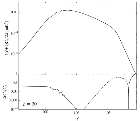
Figure 1: 21 cm angular power spectrum at redshift $30$ for a window function of width $\Delta\nu=1$ MHz without relative velocity corrections (obtained using camb sources). The bottom panel shows the relative correction when accounting for the relative velocity effect: solid lines represent an enhancement and dashed lines a suppression.

As we shall demonstrate in this paper, the relative velocity affects the 21 cm fluctuations in three different ways. First, on small scales, $k\sim 200$ Mpc^-1, the perturbations are suppressed by several tens of percent; this is because the 21 cm brightness temperature depends on the baryonic density and temperature fluctuations, which is more dramatically affected by the relative velocity than the CDM Tseliakhovich et al. (2011). Second, on extremely small scales ($k\gtrsim 2000$ Mpc^-1), we actually find an enhancement of baryonic density and temperature fluctuations, hence of 21 cm fluctuations. This comes from the quasi-resonant excitation of baryon acoustic oscillations as the baryonic fluid is advected across CDM density perturbations, an effect which was not pointed out previously. Third, and most importantly, we also find enhanced 21cm fluctuations on large scales, $k\sim 0.005-1$ Mpc^-1. This effect is less intuitive but can be summarized as follows. The relation between the 21 cm intensity and the underlying baryonic fluctuations $\delta$ is fundamentally non-linear, and we may formally write $\delta T_{21}\approx\alpha\delta+\beta\delta^{2}$, where $\alpha$ and $\beta$ are of comparable magnitude. When considering large-scale fluctuations of the brightness temperature, we therefore have $\delta T_{21}|_{l}\approx\alpha\delta_{l}+\beta(\delta^{2})_{l}$. In the absence of relative velocities, the second term would be negligible for Gaussian initial conditions and as long as perturbations are in the linear regime. However, relative velocities lead to a large-scale, order unity modulation of the amplitude of small-scale fluctuations $\delta_{s}$, and as a consequence, $(\delta^{2})_{l}\sim\langle\delta_{s}^{2}\rangle$. The small-scale fluctuations are much larger that the large-scale ones, $\delta_{l}\ll\delta_{s}\ll 1$; for $z\lesssim 100$, we even have $\delta_{s}^{2}\sim\delta_{l}$, and the quadratic term usually neglected in 21 cm fluctuations is actually comparable to the linear term, leading to an order unity enhancement of the large-scale 21 cm power spectrum. The effect on the angular power spectrum is not so dramatic, since power on large angular scales is dominated by the rapidly rising small-scale power spectrum due to standard terms. We find that the angular power spectrum is enhanced by a few percent at $z=30$ for $\ell\lesssim 1000$. We emphasize that the large-scale enhancement is formally a non-linear effect, even if the perturbations remain small. The change to the large-scale power spectrum of 21cm fluctuations is indeed of order $(\delta_{s}^{2}/\delta_{l})^{2}\sim 1$, even though $\langle\delta^{2}\rangle\ll 1$. The latter condition allows us to neglect “standard” non-linear terms which are not affected by the relative velocity.

Our results are summarized in Figure 5, where we show the standard theoretical 21 cm angular power spectrum at redshift 30 and the corrections resulting from including the relative velocity effect.

We note that several previous works have already computed the consequences of the relative velocity on the 21 cm signal in the pre-reionization era, after the first stars have formed, at redshifts $z\lesssim 30$ Bittner and Loeb (2011); Fialkov et al. (2012); Visbal et al. (2012); Fialkov et al. (2013a, b). At that epoch the relevant physical ingredients are very different than during the dark ages. On the one hand, the 21 cm spin temperature is determined by the strength of the ambient stellar ultraviolet radiation field through resonant scattering of Lyman-$\alpha$ photons (the Wouthuysen-Field effect Wouthuysen (1952); Field (1958); Hirata (2006)). On the other hand, the gas temperature, which sets the color temperature in the Lyman-$\alpha$ line, and hence the spin temperature, is determined by the rate of X-ray heating. Because the physics involved is complex, modeling the 21 cm emission from $z\lesssim 30$ requires numerical simulations, is model-dependent, and observing this signal is more likely to inform us about the details of the formation of the first luminous sources than about fundamental physics. Our work is therefore complementary to these studies, extending the physical analysis of relative velocities to higher redshifts. The 21 cm signal from the dark ages is even more challenging to observe due to ionospheric opacity and other complications Carilli et al. (2007), but can be modeled exactly, with relatively simple tools, and can potentially be a very clean probe of the very early Universe.

This paper is organized as follows. In Section II we compute the evolution of small-scale fluctuations accounting for the relative velocity of baryons and CDM. We closely follow previous works Tseliakhovich and Hirata (2010); Tseliakhovich et al. (2011) while consistently accounting for fluctuations of the free-electron fraction as in LC07. Section III describes the computation of large-scale fluctuations of quantities which depend non-linearly on the underlying density field. Finally, we apply our results to the 21 cm power spectrum from the dark ages in Section IV. We conclude in Section V. Appendix A details our method for computing autocorrelation functions of quadratic quantities, and Appendix B gives some analytic results for the angular power spectrum. All our numerical results are obtained assuming a minimal flat $\Lambda$CDM cosmology with parameters derived from Planck observations Planck Collaboration et al. (2013) $T_{\rm cmb,0}=2.726$ K, $H_{0}=67.8$ km s^-1Mpc^-1, $\Omega_{b}=0.0456$, $\Omega_{c}=0.227$, $Y_{\rm He}=0.24$, $N_{\rm eff}=3.046$, $\tau_{\rm reion}=0.089$ $A_{s}=2.196\times 10^{-9}$, $n_{s}=0.96$, $k_{\rm pivot}=0.05$ Mpc^-1.

II Effect of the relative velocity on small-scale fluctuations

II.1 Statistical properties of the relative velocity field

In this section we briefly summarize the statistical properties of the relative velocity field and the characteristic scales associated with the problem (see also TH10).

While the cold dark matter density perturbations grow unimpeded under the influence of their own gravity, baryonic matter is kinematically coupled to the photon gas by Thomson scattering until the abundance of free electrons is low enough. Using the fitting formulae of Ref. Eisenstein and Hu (1998) with the current best-fit cosmological parameters, the redshift of kinematic decoupling is $z_{\rm dec}\approx 1117$. Later on, baryons and CDM evolve as pressureless fluids on all scales greater than the baryonic Jeans scale $k_{\rm J}\sim 300$ Mpc^-1. However they have notably different initial conditions at $z_{\rm dec}$, in particular, for their peculiar velocities. In the absence of vorticity perturbations, the Fourier transform of the gauge-invariant relative velocity field takes the form

$$\boldsymbol{v}_{\rm bc}(\boldsymbol{k})\equiv\boldsymbol{v}_{\rm b}(\boldsymbol{k})-\boldsymbol{v}_{\rm c}(\boldsymbol{k})=\hat{k}\mathcal{V}(\boldsymbol{k}),$$ (1)

where from the continuity equations for baryons and CDM we have

$$\mathcal{V}(\boldsymbol{k})\equiv-\frac{1}{ik(1+z)}\frac{d}{dt}\left(\delta_{b}(\boldsymbol{k})-\delta_{c}(\boldsymbol{k})\right).$$ (2)

We define the relative velocity power spectrum $P_{v_{\rm bc}}(k)$ such that

$$\langle\mathcal{V}(\boldsymbol{k})\mathcal{V}(\boldsymbol{k^{\prime}})^{*}\rangle=(2\pi)^{3}\delta_{\rm D}(\boldsymbol{k^{\prime}}-\boldsymbol{k})P_{v_{\rm bc}}(k),$$ (3)

where $\delta_{\rm D}$ is the Dirac delta function. The variance of the relative velocity along any fixed axis is denoted by $\sigma_{1d}^{2}$. It is one third of the variance of the magnitude of the three-dimensional relative velocity vector, which we denote by $\sigma_{3d}^{2}$. They are given by

$$\sigma_{1d}^{2}\equiv\frac{1}{3}\sigma_{3d}^{2}\equiv\frac{1}{3}\int\frac{d^{3}k}{(2\pi)^{3}}P_{v_{\rm bc}}(k).$$ (4)

From symmetry considerations, the autocorrelation function of the relative velocity takes the form

$$\frac{\langle v_{\rm bc}^{i}(\boldsymbol{0})v_{\rm bc}^{j}(\boldsymbol{x})\rangle}{\sigma_{1d}^{2}}=c_{\parallel}(x)\hat{x}^{i}\hat{x}^{j}+c_{\bot}(x)(\delta^{ij}-\hat{x}^{i}\hat{x}^{j}),$$ (5)

where the dimensionless coefficients $c_{\parallel}$ and $c_{\bot}$ give the correlation of the velocity components parallel and perpendicular to the separation vector, respectively. They are given by Dalal et al. (2010)

$$c_{\parallel}(x) = \frac{1}{\sigma_{3d}^{2}}\int\frac{d^{3}k}{(2\pi)^{3}}P_{v_{\rm bc}}(k)\Big{(}j_{0}(kx)-2j_{2}(kx)\Big{)},$$ (6)

$$c_{\bot}(x) = \frac{1}{\sigma_{3d}^{2}}\int\frac{d^{3}k}{(2\pi)^{3}}P_{v_{\rm bc}}(k)\Big{(}j_{0}(kx)+j_{2}(kx)\Big{)},$$ (7)

where $j_{i}$ is the $i$-th spherical Bessel functions of the first kind. We have extracted the baryon and CDM power spectra and their derivatives at $z_{i}=1010$ from camb Lewis et al. (2000), and computed $P_{v_{\rm bc}}(k)$. We obtain $\sigma_{1d}\approx 17$ km/s and $\sigma_{3d}\approx 29$ km/s at $z_{i}$. We show the power per logarithmic interval $\Delta^{2}_{v_{\rm bc}}(k)\equiv k^{3}/(2\pi^{2})P_{v_{\rm bc}}(k)$ and the correlation coefficients of the relative velocity field in Fig. 2. After kinematic decoupling, the relative velocity decreases proportionally to $1/a$ on all scales larger than the baryonic Jeans scale since dark matter and baryons are subjected to the same acceleration on these scales Tseliakhovich and Hirata (2010).

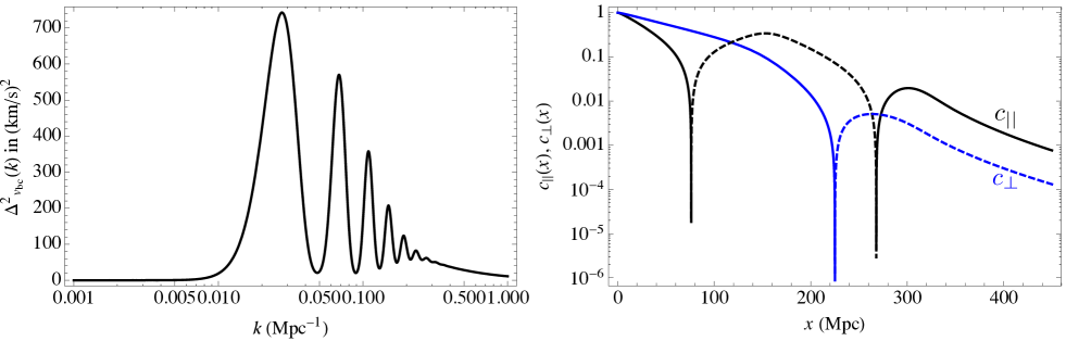
Figure 2: Statistical properties of the relative velocity field. Left: power per logarithmic $k$-interval $\Delta^{2}_{v_{\rm bc}}(k)\equiv k^{3}P_{v_{\rm bc}}(k)/(2\pi^{2})$ at redshift $z=1010$. Right: absolute value of the dimensionless auto-correlation coefficients for the relative velocity as a function of separation $x$ (solid lines for $c>0$ and dashed lines for $c<0$).

The correlation coefficients $c_{\parallel}(x),c_{\bot}(x)$ are greater than 95% for $x\lesssim 3$ Mpc and $x\lesssim 6$ Mpc, respectively, which means that the relative velocity is very nearly homogeneous on scales of a few Mpc. This defines a coherence scale for the relative velocity, $x_{\rm coh}\approx 3$ Mpc, corresponding to a wavenumber $k_{\rm coh}=(x_{\rm coh})^{-1}\approx 0.3$ Mpc^-1, which can also be inferred directly by considering the power spectrum $P_{v_{\rm bc}}(k)$.

On the other hand, starting from kinematic decoupling at time $t_{\rm dec}$, the relative velocity displaces baryons with respect to CDM perturbations by a characteristic comoving distance

$$x_{v_{\rm bc}}=\int_{t_{\rm dec}}^{t}\sigma_{1d}(t^{\prime})\frac{dt^{\prime}}{a(t^{\prime})}\approx\frac{2\sigma_{1d}(a_{\rm dec})a_{\rm dec}^{1/2}}{H_{0}\Omega_{m}^{1/2}}\approx 30\textrm{ kpc},~{}~{}$$ (8)

where in the second equality we have taken the limit $t\gg t_{\rm dec}$, assumed a matter dominated universe and used a characteristic velocity $\sigma_{1d}$ (instead of $\sigma_{3d}$) as only the component of the relative velocity along the wavevector is relevant. Baryonic fluctuations with wavenumbers $k\gtrsim 2\pi x_{v_{\rm bc}}^{-1}\approx 200$ Mpc^-1 are therefore advected across several peaks and troughs of the gravitational potential, sourced mostly by the CDM overdensity. The net acceleration partially cancels out, which slows down the growth of baryonic perturbations, and, in turn, that of the CDM. The effect is most pronounced for $k\gtrsim 200$ Mpc^-1 but it is still important at slightly larger scales, and we define $k_{v_{\rm bc}}\equiv 30$ Mpc^-1 as the typical scale at which the suppression is of the order of a percent (as we shall confirm a posteriori).

Throughout this paper, unless otherwise stated, we shall use “small scales” (and use the subscript $s$ in relation to them) to refer to scales with a wavenumber $k_{s}\gtrsim k_{v_{\rm bc}}\approx 30$ Mpc^-1, and use “large scales” (subscript $l$) for those with a wavenumber $k_{l}\lesssim k_{\rm coh}\approx 0.3$ Mpc^-1.

II.2 Basic equations

II.2.1 Moving background perturbation theory

As first pointed out in TH10 and brought to mind in the previous section, the scales at which the relative velocity affect the growth of structure are about two orders of magnitude smaller than the coherence scale of the relative velocity field. This makes it possible to use moving-background perturbation theory, i.e. compute the evolution of small-scale fluctuations given a local background value of the relative velocity. This approximation is equivalent to the eikonal approximation recently introduced in the context of cosmological perturbations Bernardeau et al. (2012, 2013). As a result, the small-scale fluctuations $\delta(\boldsymbol{k}_{s};\boldsymbol{v}_{\rm bc}(\boldsymbol{x}))$ are functions of the small-scale wavevector $\boldsymbol{k}_{s}$ and of the local relative velocity $\boldsymbol{v}_{\rm bc}(\boldsymbol{x})$. Let the reader not be confused by this mixture of Fourier-space and real-space dependence: it is justified because the relative velocity field only fluctuates significantly on large scales $k_{l}\lesssim k_{\rm coh}\ll k_{v_{\rm bc}}\lesssim k_{s}$. Moving-background perturbation theory allows us to account non-perturbatively for a fundamentally non-linear term that is active as early as $z\approx 1000$. Other non-linearities become important in the evolution of the small-scale fluctuations at lower redshifts. In this paper, we shall not concern ourselves with the latter, which can in principle be treated with standard perturbation theory methods. One should keep in mind that they do become important for the computation of 21 cm fluctuations from $z\lesssim 50$ Lewis and Challinor (2007), and should eventually be consistently included for a high-precision computation of the 21 cm signal.

Following TH10, we place ourselves in the local baryon rest-frame (defined such that the baryon velocity averaged over a few Mpc patch vanishes). We consider the evolution of small-scale modes with $k_{s}\gtrsim 30$ Mpc^-1 and can therefore neglect relativistic corrections since the scales of interest are much smaller than the horizon scale $k_{\rm hor}=aH\approx 0.001\left(\frac{1+z}{101}\right)^{1/2}$ Mpc^-1. The relative velocity is locally uniform and decreases proportionally to the inverse of the scale factor, $v_{\rm bc}\propto 1/a$.

II.2.2 Fluid equations

The linear evolution of small-scale perturbations in Fourier space is given by the usual fluid equations in an expanding universe, with an additional advection term:

$$\dot{\delta}_{c}-ia^{-1}(\boldsymbol{v}_{\rm bc}\cdot\boldsymbol{k})\delta_{c}+\theta_{c}=0,$$ (9)

$$\dot{\theta}_{c}-ia^{-1}(\boldsymbol{v}_{\rm bc}\cdot\boldsymbol{k})\theta_{c}+2H\theta_{c}-k^{2}\phi=0,~{}~{}~{}~{}$$ (10)

$$\dot{\delta}_{b}+\theta_{b}=0,$$ (11)

$$\dot{\theta}_{b}+2H\theta_{b}-\frac{k^{2}}{a^{2}}\phi-\frac{\overline{c}_{s}^{2}}{a^{2}}k^{2}\left(\delta_{b}+\delta_{T_{\rm gas}}\right)=0,$$ (12)

$$\frac{k^{2}}{a^{2}}\phi=-\frac{3}{2}\frac{H_{0}^{2}}{a^{3}}\left(\Omega_{b}^{0}\delta_{b}+\Omega_{c}^{0}\delta_{c}\right),$$ (13)

where the subscripts $b$ and $c$ refer to baryons and CDM, respectively, $\theta$ is the velocity divergence with respect to proper space, overdots denoted differentiation with respect to proper time, and $\phi$ is the Newtonian gravitational potential. In Eq. (12) $\overline{c}_{s}$ is the average baryon isothermal sound speed, given by

$$\overline{c}_{s}^{2}\equiv\frac{\overline{T}_{\rm gas}}{\mu~{}m_{\rm H}}.$$ (14)

Here $\mu$ is the mean molecular weight given by

$$\mu\equiv\frac{1+\frac{m_{\rm He}}{m_{\rm H}}x_{\rm He}}{1+x_{\rm He}+x_{e}(z)},$$ (15)

where $x_{\rm He}\equiv n_{\rm He}/n_{\rm H}$ is the constant ratio of helium to hydrogen by number and $x_{e}(z)\equiv n_{e}/n_{\rm H}$ is the free electron fraction. For a helium mass fraction $Y_{\rm He}=0.24$ and for an essentially neutral plasma, $\mu\approx 1.22$.

Following Refs. Naoz and Barkana (2005); Tseliakhovich et al. (2011), we have included matter temperature fluctuations $\delta_{T_{\rm gas}}\equiv\delta T_{\rm gas}/T_{\rm gas}$ in the baryon momentum equation (12). We do not include fluctuations of the mean molecular weight due to fluctuations of the free electron fraction as the latter is very small at the redshifts of interest, with $x_{e}\approx 5\%$ at $z=1000$ and falling below 0.1% for $z<600$.

II.2.3 Temperature fluctuations

To complete the system we need an evolution equation for $\delta_{T_{\rm gas}}$. Because some mistakes exist in the literature we rederive this equation here, following Ref. Switzer and Hirata (2008). We start by writing down the first law of thermodynamics in a small volume $V$ containing a fixed number of hydrogen nuclei (i.e. a fixed total amount of protons and neutral hydrogen atoms), so that $n_{\rm H}V$ is constant:

$$\frac{d}{dt}\left(\frac{3}{2}n_{\rm tot}VT_{\rm gas}\right)+n_{\rm tot}T_{\rm gas}\frac{dV}{dt}=\dot{Q},$$ (16)

where $n_{\rm tot}\equiv n_{\rm HI}+n_{p}+n_{e}+n_{\rm He}=n_{\rm H}(1+x_{\rm He}+x_{e})$ is the total number density of all free particles (neutral hydrogen, free protons, free electrons, and Helium), $n_{\rm H}\equiv n_{\rm HI}+n_{p}$, and $\dot{Q}$ is the rate of energy injection in the volume $V$. In the absence of any non-standard heating sources such as dark matter annihilation or decay, two sources contribute to $\dot{Q}$: photoionization / recombination and heating by CMB photons scattering off free electrons which then rapidly redistribute their energy to the rest of the gas through Coulomb scattering.

Let us first consider recombinations and photoionizations. We denote by $d\dot{x}_{e}/dE_{e}$ the differential net photoionization rate (i.e. the rate of photoionizations minus the rate of recombinations) per total abundance of hydrogen, and per interval of energy of the electron, whether it is the initial, recombining electron or the final free electron after photoionization. The source term due to recombinations and photoionizations can be written as

$$\dot{Q}_{\rm rec}=\int dE_{e}~{}E_{e}\frac{d\dot{x}_{e}}{dE_{e}}n_{\rm H}V,$$ (17)

where we used the fact that $n_{\rm H}V$ is constant. Without loss of generality we may rewrite this quantity as

$$\dot{Q}_{\rm rec} = \frac{3}{2}T_{\rm gas}\dot{x}_{e}n_{\rm H}V+\Delta\dot{Q}_{\rm rec},$$ (18)

$$\Delta\dot{Q}_{\rm rec} \equiv \int dE_{e}~{}\left(E_{e}-\frac{3}{2}T_{\rm gas}\right)\frac{d\dot{x}_{e}}{dE_{e}}n_{\rm H}V.$$ (19)

The first term in Eq. (18) contains the bulk of $\dot{Q}_{\rm rec}$, and corresponds to the rate of energy injection if every net recombination event removed on average exactly $\frac{3}{2}T_{\rm gas}$ of kinetic energy from the gas. This is nearly exact since almost all of the kinetic energy of recombining electrons goes into the emitted photon (with a very small fraction going into the recoil of the formed nucleus), and the term $\Delta\dot{Q}_{\rm rec}$ accounts for small corrections to this relation. This term is completely negligible in comparison to Compton heating and adiabatic cooling (in fact, even the much bigger term $\dot{Q}_{\rm rec}$ which was not properly included in Refs. Seager et al. (2000); Senatore et al. (2009) is negligible). Neglecting the small correction term $\Delta\dot{Q}_{\rm rec}$, after simplification we get the evolution equation for the gas temperature

$$\dot{T}_{\rm gas}-\frac{2}{3}\frac{\dot{n}_{\rm H}}{n_{\rm H}}T_{\rm gas}=\frac{2}{3}\dot{q}_{\rm C},$$ (20)

where $\dot{q}_{\rm C}$ is the Compton heating rate per particle:

$$\dot{q}_{\rm C} = \frac{4\sigma_{\rm T}a_{r}T_{\rm cmb}^{4}}{(1+x_{\rm He}+x_{e})m_{e}}x_{e}(T_{\rm cmb}-T_{\rm gas})$$ (21)

$$\equiv \frac{3}{2}\Gamma_{\rm C}\frac{x_{e}}{\overline{x}_{e}}(T_{\rm cmb}-T_{\rm gas}).$$

Here $\sigma_{\rm T}$ is the Thomson cross-section, $a_{r}$ is the radiation constant, $m_{e}$ is the electron mass, and we have defined the rate

$$\Gamma_{\rm C}\equiv\frac{8\sigma_{\rm T}a_{r}T_{\rm cmb}^{4}}{3(1+x_{\rm He}+x_{e})m_{e}}\overline{x}_{e},$$ (22)

which we shall assume to be homogeneous as it only depends on the local free electron fraction through the term $1+x_{\rm He}+x_{e}\approx 1+x_{\rm He}$. The homogeneous part of Eq. (20) gives the evolution of the average matter temperature:

$$\dot{\overline{T}}_{\rm gas}+2H\overline{T}_{\rm gas}=\Gamma_{\rm C}(T_{\rm cmb}-\overline{T}_{\rm gas}).$$ (23)

We now turn to the perturbations. Assuming the helium to hydrogen ratio is uniform, and up to very small corrections of order $x_{e}\times(m_{e}/m_{p})$, we have $\delta n_{\rm H}/n_{\rm H}=\delta_{b}$. Since we are considering scales deep inside the Horizon, photon temperature perturbations are negligible compared to any other perturbations, and we set $T_{\rm cmb}=\overline{T}_{\rm cmb}$. The non-perturbative evolution equation for the gas temperature fluctuation therefore reads:

$$\dot{\delta}_{T_{\rm gas}}-\frac{2}{3}\dot{\delta}_{b}\frac{1+\delta_{T_{\rm gas}}}{1+\delta_{b}}=$$

$$\Gamma_{\rm C}\left[\frac{\overline{T}_{\rm cmb}-\overline{T}_{\rm gas}}{\overline{T}_{\rm gas}}\delta_{x_{e}}-\left(\frac{\overline{T}_{\rm cmb}}{\overline{T}_{\rm gas}}+\delta_{x_{e}}\right)\delta_{T_{\rm gas}}\right],$$ (24)

which corresponds to Eq. (16) of Ref. Pillepich et al. (2007) if $\delta_{x_{e}}\equiv\delta x_{e}/\overline{x}_{e}=0$. To first order, the evolution equation for the temperature perturbations is therefore

$$\dot{\delta}_{T_{\rm gas}}-\frac{2}{3}\dot{\delta}_{b}=\Gamma_{\rm C}\left[\frac{\overline{T}_{\rm cmb}-\overline{T}_{\rm gas}}{\overline{T}_{\rm gas}}\delta_{x_{e}}-\frac{\overline{T}_{\rm cmb}}{\overline{T}_{\rm gas}}\delta_{T_{\rm gas}}\right].~{}~{}~{}~{}~{}$$ (25)

Refs. Naoz and Barkana (2005); Tseliakhovich et al. (2011) did not account for the fluctuations of the free-electron fraction. This is justified at high redshifts at which the matter temperature is very close to the radiation temperature and the prefactor of $\delta_{x_{e}}$ in Eq. (25) is small; it is also justified at $z\ll 200$ when $\Gamma_{\rm C}\ll H$ and the gas simply cools adiabatically. However, at intermediate stages this term cannot be neglected, at least formally. Besides our neglect of photon temperature perturbations and relativistic corrections (of order $\sim a^{2}H^{2}/k^{2}\delta_{m}\ll\delta_{m}$ in the deep sub-horizon regime), our equation (25) is identical to Eq. (B12) of LC07, and does not include spurious molecular weight terms as in Ref. Senatore et al. (2009), where the term $\dot{Q}_{\rm rec}$ was not accounted for.

In order to account for other potential heating sources such as dark matter annihilation Chen and Kamionkowski (2004); Giesen et al. (2012), one would simply have to add the corresponding heating rate to the right-hand side of Eq. (20), and perturb the equation consistently Dvorkin et al. (2013).

II.2.4 Free-electron fraction fluctuations

To close our system of equations we require an evolution equation for the fluctuations in the ionization fraction of the gas. Because the pre-factor of $\delta_{x_{e}}$ in Eq. (25) is less than 1% for $z\gtrsim 500$ Ali-Haïmoud and Hirata (2011), we only need to have an accurate equation at late times and we do not need to worry about details of the radiative transfer in the Lyman-$\alpha$ line, which affect the recombination history near the peak of the CMB visibility function (see for example Refs. Hirata and Forbes (2009); Chluba and Sunyaev (2010) and references therein). We compute the background recombination history exactly with hyrec Ali-Haïmoud and Hirata (2011) but when computing the perturbations, we simply adopt an effective 3-level atom model Peebles (1968); Zel’dovich et al. (1969), for which the recombination rate is given by

$$\dot{x}_{e}=-C\left(\mathcal{A}_{\rm B}n_{\rm H}x_{e}^{2}-4(1-x_{e})\mathcal{B}_{\rm B}\textrm{e}^{-E_{21}/T_{\rm cmb}}\right),$$ (26)

where $E_{21}=10.2$ eV is the energy of the Lyman-$\alpha$ transition, $\mathcal{A}_{\rm B}(T_{\rm cmb},T_{\rm gas})$ is the effective case-B recombination coefficient, $\mathcal{B}_{\rm B}(T_{\rm cmb})$ is the corresponding effective photoionization rate, and $C$ is the Peebles C-coefficient Peebles (1968), which gives the ratio of the net rate of downward transitions from the first excited states to their total effective lifetime:

$$C \equiv \frac{3R_{\rm Ly\alpha}+\Lambda_{2s,1s}}{3R_{\rm Ly\alpha}+\Lambda_{2s,1s}+4\mathcal{B}_{\rm B}},$$ (27)

$$R_{\rm Ly\alpha} \equiv \frac{8\pi(H+\frac{1}{3}\theta_{b})}{3\lambda_{\rm Ly\alpha}^{3}(1-x_{e})n_{\rm H}}.$$ (28)

Equation (26) is identical in spirit to that of Peebles Peebles (1968) and of Ref. Seager et al. (2000), with however two technical differences. First, following LC07 and Ref. Senatore et al. (2009), we have replaced the Hubble rate in the Lyman-$\alpha$ escape rate (28) by the local expansion rate, which is enhanced by one third of the baryon peculiar velocity divergence. This simple replacement relies on the implicit assumption that the recombination process is local, in the sense that the Lyman-$\alpha$ radiation field is determined by the density and temperature within a distance much smaller than the wavelength of the scales considered. Checking this assumption quantitatively is non trivial, however at the low redshifts of interest the net recombination rate is independent of the details of the Lyman-$\alpha$ radiative transfer ($C\rightarrow 1$ for $z\lesssim 900$), and the detailed value of the perturbed $C$-factor is not critical.

Second, instead of using the case-B recombination coefficient $\alpha_{\rm B}(T_{\rm gas})$ of Ref. Pequignot et al. (1991) or a fudged version of it as in Ref. Seager et al. (2000), we use the effective recombination coefficient $\mathcal{A}_{\rm B}(T_{\rm gas},T_{\rm cmb})$, which accounts exactly for stimulated recombinations to, ionizations from, and transitions between, the highly-excited states of hydrogen during the cascading process Ali-Haïmoud and Hirata (2010). These coefficients are related through $\alpha_{\rm B}=\mathcal{A}_{\rm B}(T_{\rm cmb}=0)$. The temperature dependence of $\alpha_{\rm B}$ (even rescaled by a fudge factor) differs from the correct one given by $\mathcal{A}_{\rm B}$ at the level of $\sim 10-20$%.

For $z<1010$ the free-electron fraction is already much larger than its value in Saha equilibrium and the second term in Eq. (26) is less than $10^{-4}$ times the first term. We therefore have, to an excellent accuracy,

$$\dot{x}_{e}\approx-C\mathcal{A}_{\rm B}n_{\rm H}x_{e}^{2}.$$ (29)

This allows us to get a simple expressions for the evolution of $\delta_{x_{e}}$, to first order:

$$\dot{\delta}_{x_{e}} = \frac{\dot{\overline{x}}_{e}}{\overline{x}_{e}}\Bigg{[}\delta_{x_{e}}+\delta_{b}+\frac{\partial\ln\mathcal{A}_{\rm B}}{\partial\ln T_{\rm gas}}\delta_{T_{\rm gas}}$$ (30)

$$~{}~{}~{}~{}~{}+\frac{\partial\ln C}{\partial\ln R_{\rm Ly\alpha}}\left(\frac{\theta_{b}}{3H}-\delta_{b}\right)\Bigg{]},$$

where we have used the fact that $C$ depends on the baryon density and velocity divergence $\theta_{b}$ through the Lyman$-\alpha$ escape probability, and we have neglected fluctuations of the free electron fraction in the Lyman-$\alpha$ escape rate since $x_{e}\ll 1$ at the times of interest.

Here again, one can easily include additional ionization sources, for example resulting from dark matter annihilation Chen and Kamionkowski (2004); Giesen et al. (2012); Dvorkin et al. (2013).

II.2.5 Initial conditions

The initial conditions for $\delta_{b},\theta_{b},\delta_{c}$ and $\theta_{c}$ are extracted from camb at $z_{\rm ini}=1010$. The initial condition for $\delta_{T_{\rm gas}}$ is obtained from noticing that at $z_{\rm ini}$, $H/\Gamma_{\rm C}\approx 3\times 10^{-5}\ll 1$, and $T_{\rm gas}\approx T_{\rm cmb}$ to an excellent accuracy. Up to corrections of order $\dot{\delta}_{b}/\Gamma_{\rm C}\ll\delta_{b}$ and $\delta_{T_{\rm cmb}}$, we therefore have $\delta_{T_{\rm gas}}(z_{\rm init})=0$.

In principle one should start computing the evolution of ionization fraction perturbations from an earlier time in order to get the proper initial conditions at $z_{\rm ini}=1010$. However, since the perturbations of $\delta_{x_{e}}$ only affect the 21 cm signal at late times through their coupling to $\delta_{T_{\rm gas}}$, and since the entire system is driven by $\delta_{c}\gg\delta_{x_{e}}\sim\delta_{b}$ initially, the value of $\delta_{x_{e}}(z_{\rm ini})$ is quickly forgotten and has virtually no effect on the observables of interest here. We may therefore safely set $\delta_{x_{e}}(z_{\rm init})=0$.

II.3 Results: evolution of small-scale fluctuations

We have numerically solved the coupled differential equations (9)-(13), (25) and (30) for $\delta_{b},\delta_{c},\delta_{T_{\rm gas}}$ and $\delta_{x_{e}}$, as a function of $k$ and $\boldsymbol{v}_{\rm bc}(z_{\rm dec})\cdot\hat{k}$, starting at $z_{\rm ini}=1010$ with initial conditions described above, down to $z=20$. The evolution of the background free-electron fraction and matter temperature is computed with the recombination code hyrec.

We show the evolution of the baryon density fluctuations $\delta_{b}$ for two modes in Fig. 3. For a scale $k=200$ Mpc^-1 of the order of the advection scale but somewhat larger than the Jeans scale ($k_{\rm Jeans}\approx 300$ Mpc^-1), the relative velocity destroys the phase coherence between baryons and dark matter by advecting their perturbations across more than a wavelength in a Hubble time. The result is to suppress the growth of structure, as illustrated in the left panel of Fig. 3. On the other hand, for scales much smaller than the Jeans scale, we find that a typical value of the relative velocity actually leads to a resonant amplification of baryon density and temperature fluctuations (see evolution of the mode $k=2700$ Mpc^-1 in Fig. 3). This can be understood as follows. On sub-Jeans scales, baryonic fluctuations are suppressed due to their pressure support, and $\delta_{b}\ll\delta_{c}$. One can solve explicitly for the evolution of the growing mode of CDM perturbation in the limit $\delta_{b}=0$ and obtain, during matter domination:

$$\delta_{c} \propto \exp\left[i\boldsymbol{k}\cdot\int^{t}\frac{\boldsymbol{v}_{\rm bc}}{a}dt\right]a^{\alpha},$$ (31)

$$\alpha \equiv 1-\frac{5}{4}\left(1-\sqrt{1-\frac{24}{25}f_{b}}\right)\approx 1-\frac{3}{5}f_{b},$$ (32)

$$f_{b} \equiv \frac{\Omega_{b}}{\Omega_{c}+\Omega_{c}},$$ (33)

where the approximate value of the growth rate in Eq. (32) is valid in the limit $f_{b}\ll 1$. With our fiducial cosmology $f_{b}\approx 0.17$ and $\alpha\approx 0.90$. Baryonic perturbations undergo acoustic oscillations forced by the gravitational attraction from the dark matter and damped by the Hubble expansion:

$$\ddot{\delta}_{b}+2H\dot{\delta}_{b}+\frac{\overline{c}_{s}^{2}}{a^{2}}k^{2}\left(1+\frac{\delta_{T_{\rm gas}}}{\delta_{b}}\right)\delta_{b}=\frac{3}{2}H^{2}(1-f_{b})\delta_{c}.$$ (34)

Figure 4 shows that the characteristic relative velocity along a given axis is very close to the adiabatic sound speed for $z\lesssim 200$. For typical relative velocities, the forcing term in Eq. (34) therefore oscillates with a frequency close to that of acoustic oscillations, which leads to a resonant amplification of acoustic waves.

Figure 5 shows the evolution of the ratio $|\delta_{T_{\rm gas}}/\delta_{b}|$ for $k=200$ Mpc^-1 and $k=2700$ Mpc^-1. We see that the relative velocity leads to a faster convergence to the adiabatic regime $\delta_{T_{\rm gas}}\rightarrow\frac{2}{3}\delta_{b}$, with a very pronounced effect for scales much smaller than the Jeans scale. This can be understood by considering Eq. (25), neglecting fluctuations of the free electron fraction for simplicity. In this equation, the term $\frac{2}{3}\dot{\delta}_{b}$ can be seen as a forcing term; physically, it arises from the work done by the compression and expansion of the baryonic fluid. The term linear in $\delta_{T_{\rm gas}}$ is a friction term, which translates the tendency for the gas temperature to equilibrate with the (nearly) homogeneous CMB temperature through Thomson scattering. In the deep sub-Jeans regime the baryonic overdensity oscillates in time like its own forcing term (31), so that $\dot{\delta}_{b}\sim(\boldsymbol{k}\cdot\boldsymbol{v}_{\rm bc}/a)\delta_{b}$, which increases with wavenumber. For very small scales, this term can be much larger than the friction term, in which case the gas temperature fluctuation rapidly equilibrates to 2/3 of the baryon density fluctuations.

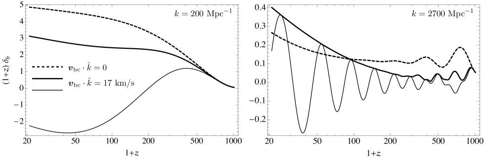
Figure 3: Evolution of $\delta_{b}(k,z)$ for two small-scale modes with $k=200$ Mpc^-1 and $k=2700$ Mpc^-1 (specifically, what is plotted is $(1+z)T_{\delta_{b}}(k,z)[A_{s}(k/k_{\rm pivot})^{n_{s}-1}]^{1/2}$, where $T_{\delta_{b}}(k,z)$ is the transfer function). The values of the relative velocity are $\boldsymbol{v}_{\rm bc}\cdot\hat{k}=0$ (dotted) and $\boldsymbol{v}_{\rm bc}\cdot\hat{k}=17$ km/s (solid), the latter corresponding to the rms relative velocity along a given axis. Thick lines represent the absolute value of $\delta_{b}$ and thin lines show its real part (the two quantities are equal for $\boldsymbol{v}_{\rm bc}\cdot\hat{k}=0$). For $k=200$ Mpc^-1 the relative velocity leads to a suppression of fluctuations, whereas for $k=2700$ Mpc^-1 the streaming of baryons relative to the dark matter leads to a resonant amplification of baryonic acoustic oscillations.

Figure 4: Rms value of the relative velocity along a given axis (solid line) compared to the adiabatic sound speed $\overline{c}_{s}^{\rm ad}=\sqrt{5/3}~{}\overline{c}_{s}^{\rm iso}$ (dashed line), as a function of redshift.

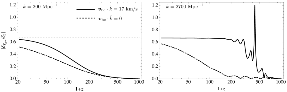
Figure 5: Evolution of the ratio $|\delta_{T_{\rm gas}}/\delta_{b}|$ as a function of redshift, for $k=200$ Mpc^-1 and $k=2700$ Mpc^-1, as a function of the local relative velocity. In both cases the relative velocity speeds up the convergence towards the adiabatic limit $\delta_{T_{\rm gas}}=\frac{2}{3}\delta_{b}$ (indicated with a dotted line). The effect is much more pronounced for very small scales.

In Fig. 6 we show the small-scale power spectra of the baryon density and temperature fluctuations at $z=50$, both in the standard case (setting $\boldsymbol{v}_{\rm bc}=0$), and averaged over the Gaussian distribution of the relative velocity vector. The latter is most efficiently computed by averaging over the one-dimensional distribution of $\boldsymbol{v}_{\rm bc}\cdot\hat{k}$. We have checked that our result for the total matter power spectrum agrees with that of TH10. We have also checked that our results are in good agreement with those of camb when setting $\boldsymbol{v}_{\rm bc}=0$. The main effect of the relative velocity is to suppress power by several tens of percent on scales $k\sim 100-300$ Mpc^-1, and enhance it on very small scales for which baryon acoustic oscillations get resonantly forced. The transition from suppression to enhancement occurs at larger scales for the temperature fluctuations, due to the faster convergence to the adiabatic regime described above.

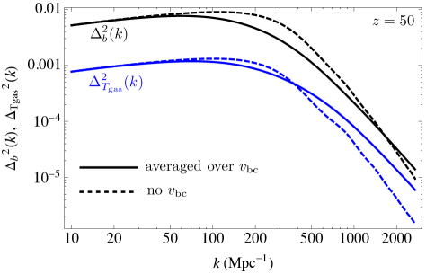
Figure 6: Power per logarithmic $k$-interval for baryon density and temperature fluctuations at $z=50$, neglecting the relative velocities (dashed lines), and averaging over their probability distribution (solid lines). Accounting for relative velocities leads to a suppression of power around $k\sim 200$ Mpc^-1 and an enhancement at smaller scales due to resonant excitation of acoustic waves. The enhancement is more pronounced for temperature fluctuations, which are driven towards the adiabatic regime $\delta_{T_{\rm gas}}\rightarrow\frac{2}{3}\delta_{b}$ earlier on when relative velocities are present.

III Modulation of non-linear quantities on large scales

III.1 Motivation

The 21 cm brightness temperature is a non-linear function of the baryon density and temperature (see Section IV for details). In addition, as can be seen from Eq. (20), the gas temperature itself depends non-linearly on the gas density. The goal of this section is to show how the large-scale fluctuations of the relative velocity between baryons and CDM leads to a large-scale modulation of non-linear quantities, which can be comparable to the large-scale fluctuations of linear perturbations.

Let us consider a quantity $X(\rho_{b})$ that depends non-linearly on the local baryon density $\rho_{b}(\boldsymbol{x})\equiv\overline{\rho}_{b}(1+\delta(\boldsymbol{x}))$. The following argument can be immediately generalized to a dependence on multiple perturbations, such as density, temperature or ionization fraction. Since during the dark ages $\delta\ll 1$ on all scales, we may write $X$ as a Taylor expansion:

$$X\left(\rho_{b}(\boldsymbol{x})\right)=\chi_{0}+\chi_{1}\delta(\boldsymbol{x})+\chi_{2}\delta(\boldsymbol{x})^{2}+\mathcal{O}(X\delta^{3}),$$ (35)

where the coefficients $\chi_{0},\chi_{1},\chi_{2}$ are functions of redshift only and are in general of comparable magnitude. We now decompose the density fluctuation in a long-wavelength part and a short-wavelength part:

$$\delta(\boldsymbol{x})=\delta_{l}(\boldsymbol{x})+\delta_{s}(\boldsymbol{x}).$$ (36)

Both $\delta_{l}$ and $\delta_{s}$ are small quantities; however, there exists a hierarchy between them:

$$\delta_{l}\ll\delta_{s}\ll 1.$$ (37)

In fact, for $z\lesssim 100$, taking $k_{s}\sim 100$ Mpc^-1 and $k_{l}\sim 0.01$ Mpc^-1, the hierarchy between long- and short-wavelength fluctuations is such that

$$\delta_{s}^{2}\sim\delta_{l}.$$ (38)

We therefore ought to write a two-parameter Taylor expansion of $X$. To first order in $\delta_{l}$ and second order in $\delta_{s}$, we have

$$X(\rho)=\chi_{0}+\chi_{1}(\delta_{l}+\delta_{s})+\chi_{2}\delta_{s}^{2}+\mathcal{O}(X\delta_{s}\delta_{l}).$$ (39)

If we consider the small-scale fluctuations of $X$, we see that, to lowest order,

$$X_{s}=\chi_{1}\delta_{s}+\mathcal{O}(X\delta_{s}^{2}),$$ (40)

i.e. at small scales we only need to account for the linear term, up to corrections of relative order $\delta_{s}$. However, when computing the long-wavelength fluctuations of $X$, the quadratic term does become important and can be comparable to the linear term, provided it is significantly modulated on large scales:

$$X_{l}=\chi_{1}\delta_{l}+\chi_{2}(\delta_{s}^{2})_{l}+\mathcal{O}(X\delta_{s}^{3},X\delta_{l}^{2}).$$ (41)

In the absence of relative velocities, $\delta_{s}^{2}$ does vary stochastically, but mostly on small scales. On the other hand, fluctuations of the relative velocity over large scales lead to order unity fluctuations of the small-scale power spectrum, and therefore $(\delta_{s}^{2})_{l}\sim\delta_{s}^{2}\sim\delta_{l}$. This is illustrated in Fig. 7.

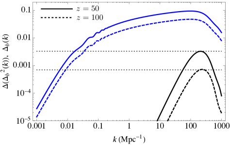
Figure 7: Characteristic change in the small-scale baryon power $\Delta(\Delta_{b}^{2}(k))\equiv|\langle\Delta_{b}^{2}(k)\rangle-\Delta_{b}^{2}(k,v_{\rm bc}=0)|$ (black, lower two curves) and characteristic baryon overdensity $\Delta_{b}(k)\equiv\left[k^{3}P_{b}(k)/(2\pi^{2})\right]^{1/2}$ (blue, upper two curves), as a function of wavenumber, and at redshifts 100 and 50. The dotted lines illustrate that the long-wavelength modulation of the small-scale quadratic fluctuations is of the same order as the long-wavelength fluctuations of the linear overdensity: $(\delta_{s}^{2})_{l}=\Delta\delta_{s}^{2}\sim\delta_{l}$.

In order to compute the long-wavelength fluctuation of $\delta_{s}^{2}$, we may first smooth it over an intermediate scale of a few tenths of Mpc, such that the smoothing scale satisfies

$$k_{\rm coh}\ll k_{\rm smooth}\ll k_{v_{\rm bc}}.$$ (42)

The first inequality ensures that the long-wavelength fluctuations of the field are unaffected by smoothing: denoting the smoothed field by $\widetilde{\delta_{s}^{2}}$, we have $(\delta_{s}^{2})_{l}\approx(\widetilde{\delta_{s}^{2}})_{l}$, up to corrections of order $(k_{l}/k_{\rm smooth})^{2}$ with a Gaussian smoothing kernel. The second inequality allows us to replace the spatial averaging involved in the smoothing by a statistical averaging:

$$\widetilde{\delta_{s}^{2}}\approx\overline{\delta_{s}^{2}}(v_{\rm bc})\equiv\int\frac{d^{3}k_{s}}{(2\pi)^{3}}P_{\delta}(\boldsymbol{k}_{s},\boldsymbol{v}_{\rm bc}).$$ (43)

Finally, the fluctuating part is obtained by subtracting the average over the Gaussian distribution of relative velocities:

$$(\delta_{s}^{2})_{l}(v_{\rm bc})=\Delta\delta_{s}^{2}\equiv\overline{\delta_{s}^{2}}(v_{\rm bc})-\big{\langle}\overline{\delta_{s}^{2}}\big{\rangle}.$$ (44)

As an illustration, we show the fluctuation of the variance $\overline{\delta_{s}^{2}}(v_{\rm bc})$ as a function of the relative velocity, and at several redshifts in Fig. 8.

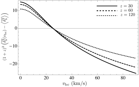
Figure 8: Variation of the variance of the small-scale baryon overdensity as a function of the magnitude of the local relative velocity, at $z=30,60$ and 120. We have multiplied $\delta_{b}^{2}$ by $(1+z)^{2}$ in order to factor out the approximately linear growth of overdensities with the scale factor during matter domination (in practice the growth rate is slightly faster than linear with the scale factor as baryons fall in the pre-existing dark matter potential wells).

III.2 Correlation functions and power spectra

In this section we give a more detailed and quantitative description of the method to compute statistical properties of non-linear quantities, accounting for the relative velocity effect. A summary of this section can be found in paragraph III.2.5.

III.2.1 Probability distribution for the overdensity

We first need to determine the joint probability distribution for the overdensity pair $(\delta_{0},\delta_{x})$ at two points with separation $\boldsymbol{x}$. We start by describing the constrained distribution $\mathcal{P}(\delta_{0},\delta_{x}|\boldsymbol{v}_{0},\boldsymbol{v}_{x})$: the probability of the pair $(\delta_{0},\delta_{x})$ given fixed values of the relative velocities $\boldsymbol{v}_{0}\equiv\boldsymbol{v}_{\rm bc}(\boldsymbol{0})$ and $\boldsymbol{v}_{x}\equiv\boldsymbol{v}_{\rm bc}(\boldsymbol{x})$. From there the full distribution $\mathcal{P}(\delta_{0},\delta_{x})$ is obtained by convolving with the six-dimensional joint Gaussian probability distribution for $(\boldsymbol{v}_{0},\boldsymbol{v}_{x})$, which we denote by $\mathcal{P}(\boldsymbol{v}_{0},\boldsymbol{v}_{x})$, i.e.

$$\mathcal{P}(\delta_{0},\delta_{x})=\int d^{3}v_{0}d^{3}v_{x}\mathcal{P}(\boldsymbol{v}_{0},\boldsymbol{v}_{x})\mathcal{P}(\delta_{0},\delta_{x}|\boldsymbol{v}_{0},\boldsymbol{v}_{x}).$$ (45)

Throughout this section an overline $\overline{X}$ denotes the averaging with respect to the distribution of overdensities at fixed values of the relative velocities and brackets $\langle.\rangle$ denote the subsequent averaging over the distribution of relative velocities.

We decompose the density field into its small-scale contribution $\delta_{s}$, which only contains modes with $k\geq k_{v_{\rm bc}}$ and its long-wavelength contribution $\delta_{l}\equiv\delta-\delta_{s}$ (here $\delta_{l}$ includes not only large-scale modes but all modes with $k\leq k_{v_{\rm bc}}$).

The distribution of the small-scale modes $\mathcal{P}_{s}$ is a two-dimensional Gaussian with vanishing means and variances $\overline{\delta_{0s}^{2}}(v_{0}),\overline{\delta_{xs}^{2}}(v_{x})$ obtained from

$$\overline{\delta_{s}^{2}}(v_{\rm bc})\equiv\int_{k\geq k_{v_{\rm bc}}}\frac{d^{3}k}{(2\pi)^{3}}P_{\delta}(\boldsymbol{k},\boldsymbol{v}_{\rm bc}).$$ (46)

Since $\delta_{s}$ has support only on $k\geq k_{v_{\rm bc}}$, the covariance $\overline{\delta_{0s}\delta_{xs}}$ rapidly vanishes for $x\gtrsim$ few $k_{v_{\rm bc}}^{-1}\ll x_{\rm coh}$. It is therefore only significant for separations well within the coherence scale of the relative velocity, for which $\boldsymbol{v}_{0}=\boldsymbol{v}_{x}$. It can be computed at all separations by Fourier transforming either $P(\boldsymbol{k},\boldsymbol{v}_{0})$ or $P(\boldsymbol{k},\boldsymbol{v}_{x})$:

$$\overline{\delta_{0s}\delta_{xs}}(\boldsymbol{x},\boldsymbol{v}_{0})=\int_{k\geq k_{v_{\rm bc}}}\frac{d^{3}k}{(2\pi)^{3}}\textrm{e}^{i\boldsymbol{k}\cdot\boldsymbol{x}}P_{\delta}(\boldsymbol{k},\boldsymbol{v}_{0}).$$ (47)

It will be useful in what follows to understand the symmetries of this function. First, consideration of the system (9)-(13) shows that the transfer function of the overdensity is a function of $k$ and $\hat{k}\cdot\boldsymbol{v}_{\rm bc}$ only, and so will be the power spectrum. Moreover, the complex conjugate $\delta^{*}(k,\hat{k}\cdot\boldsymbol{v}_{\rm bc})=\delta(k,-\hat{k}\cdot\boldsymbol{v}_{\rm bc})$, which implies that the power spectrum depends on $k$ and the absolute value $|\boldsymbol{k}\cdot\boldsymbol{v}_{\rm bc}|$, i.e. is symmetric in $\boldsymbol{v}_{\rm bc}$. This implies that the correlation function $\overline{\delta_{0s}\delta_{xs}}$ is a function of $x,v_{\rm bc}$ and $|\boldsymbol{x}\cdot\boldsymbol{v}_{\rm bc}|$ only, and is also an even function of $\boldsymbol{v}_{\rm bc}$.

The large-scale pieces $(\delta_{0l},\delta_{xl})$ have a priori non-zero correlations with the relative velocity field. Specifically, symmetry considerations show that the non-vanishing correlations are $\langle\delta_{0l}v_{x,||}\rangle=-\langle\delta_{xl}v_{0,||}\rangle$, where $v_{i||}\equiv\boldsymbol{v}_{i}\cdot\hat{x}$ is the projection of the relative velocity along the separation vector. For given values of the relative velocity, the distribution $\mathcal{P}_{l}$ is therefore a constrained Gaussian, with means

$$\overline{\delta_{0}}=\frac{\langle\delta_{0}v_{x||}\rangle}{(1-c_{||}^{2})\sigma_{1d}^{2}}\left(v_{x||}-c_{||}v_{0||}\right),$$ (48)

$$\overline{\delta_{x}}=\frac{\langle\delta_{x}v_{0||}\rangle}{(1-c_{||}^{2})\sigma_{1d}^{2}}\left(v_{0||}-c_{||}v_{x||}\right),$$ (49)

where we have dropped the subscripts “$l$” since these expressions are also valid for the total overdensity. The covariance matrix has elements

$$\overline{\delta_{0l}^{2}}-\left(\overline{\delta_{0}}\right)^{2} = \langle\delta_{l}^{2}\rangle-\frac{\langle\delta_{0}v_{x||}\rangle^{2}}{(1-c_{||}^{2})\sigma_{1d}^{2}},$$ (50)

$$\overline{\delta_{xl}^{2}}-\left(\overline{\delta_{x}}\right)^{2} = \langle\delta_{l}^{2}\rangle-\frac{\langle\delta_{x}v_{0||}\rangle^{2}}{(1-c_{||}^{2})\sigma_{1d}^{2}},$$ (51)

$$\overline{\delta_{0l}\delta_{xl}}-\overline{\delta_{0}}\times\overline{\delta_{x}} = \langle\delta_{0l}\delta_{xl}\rangle+c_{||}\frac{\langle\delta_{0}v_{x||}\rangle\langle\delta_{x}v_{0||}\rangle}{(1-c_{||}^{2})\sigma_{1d}^{2}},$$ (52)

where the right-hand sides are independent of the relative velocities $(\boldsymbol{v}_{0},\boldsymbol{v}_{x})$.

For a given pair of relative velocities $(\boldsymbol{v}_{0},\boldsymbol{v}_{x})$, the small-scale parts $(\delta_{0s},\delta_{0x})$ and the large-scale parts $(\delta_{0l},\delta_{xl})$ are independent pairs of variables, so that we may rewrite the probability distribution for $(\delta_{0},\delta_{x})$ given $(\boldsymbol{v}_{0},\boldsymbol{v}_{x})$ as

$$\mathcal{P}(\delta_{0},\delta_{x}|\boldsymbol{v}_{0},\boldsymbol{v}_{x})=\int d\delta_{0s}d\delta_{xs}\mathcal{P}_{s}(\delta_{0s},\delta_{xs}|\boldsymbol{v}_{0},\boldsymbol{v}_{x})$$

$$\times\mathcal{P}_{l}(\delta_{0}-\delta_{0s},\delta_{x}-\delta_{xs}|\boldsymbol{v}_{0},\boldsymbol{v}_{x}).$$ (53)

As a consequence, at fixed relative velocities, the sums $\delta_{0}=\delta_{0s}+\delta_{0l}$, $\delta_{x}=\delta_{xs}+\delta_{xl}$ also have a two dimensional Gaussian distribution, whose first and second order moments are just the sums of those of $\mathcal{P}_{s}$ and $\mathcal{P}_{l}$.

The independence of small-scale and large scale modes is only valid at fixed relative velocities and no longer holds after convolution with the probability distribution of relative velocities to obtained the full probability distribution of $(\delta_{0},\delta_{x})$ through Eq. (45).

When computing the cosmic average $\langle\overline{F}\rangle$ of a function $F(\delta_{0},\delta_{x})$, we must evaluate the integral

$$\Big{\langle}\overline{F(\delta_{0},\delta_{x})}\Big{\rangle}\equiv\int d\delta_{0}d\delta_{x}\mathcal{P}(\delta_{0},\delta_{x})F(\delta_{0},\delta_{x}).$$ (54)

After a change of variables we arrive at

$$\Big{\langle}\overline{F(\delta_{0},\delta_{x})}\Big{\rangle}=\Big{\langle}\overline{F(\delta_{0s}+\delta_{0l},\delta_{xs}+\delta_{xl})}\Big{\rangle},$$ (55)

where the first averaging, denoted by an overline, is to be performed over the independent distributions of $(\delta_{0s},\delta_{xs})$ and $(\delta_{0l},\delta_{xl})$ at fixed relative velocities, and is followed by averaging over the distribution of velocities, denoted by brackets. With this probability distribution at hand, we may compute various correlation functions. This will allow us to compute the autocorrelation function and power spectrum of 21 cm fluctuations in the next section.

III.2.2 Autocorrelation of the density field

Let us start by computing the autocorrelation of the density field:

$$\xi_{\delta}(x)\equiv\Big{\langle}\overline{\delta_{0}\delta_{x}}\Big{\rangle} = \Big{\langle}\overline{(\delta_{0s}+\delta_{0l})(\delta_{xs}+\delta_{xl})}\Big{\rangle}$$ (56)

$$= \Big{\langle}\overline{\delta_{0s}\delta_{xs}}\Big{\rangle}+\Big{\langle}\overline{\delta_{0l}\delta_{xl}}\Big{\rangle},$$

where we have used the independence of small-scale and large-scale modes at fixed relative velocity. The second avergage is just $\langle\delta_{0l}\delta_{xl}\rangle$, obtained from Fourier transforming $P(k<k_{v_{\rm bc}})$, which is independent of the relative velocity. The average of the small-scale correlation function is obtained from averaging Eq. (47) over the distribution of $\boldsymbol{v}_{0}$, which amounts to taking the Fourier transform of the velocity-averaged small-scale power spectrum. We therefore arrive at

$$\xi_{\delta}(x)=\int\frac{d^{3}k}{(2\pi)^{3}}\textrm{e}^{i\boldsymbol{k}\cdot\boldsymbol{x}}\langle P_{\delta}(\boldsymbol{k},\boldsymbol{v}_{0})\rangle.$$ (57)

By taking the Fourier transform, we see that the full-sky power spectrum is simply obtained by averaging the local power spectrum over the distribution of relative velocities, as one may expect intuitively.

III.2.3 Autocorrelation of the density field squared

We now compute the autocorrelation function of $\delta^{2}$:

$$\xi_{\delta^{2}}(x)\equiv\Big{\langle}\overline{\delta_{0}^{2}\delta_{x}^{2}}\Big{\rangle}-\Big{\langle}\overline{\delta^{2}}\Big{\rangle}^{2}.$$ (58)

Using Wick’s theorem for the Gaussian variables $(\delta_{0},\delta_{x})$ at fixed relative velocities (and accounting for the non-zero means), we arrive at

$$\xi_{\delta^{2}}(x) = 2\bigg{\langle}\Big{(}\overline{\delta_{0}\delta_{x}}\Big{)}^{2}-\Big{(}\overline{\delta_{0}}\times\overline{\delta_{x}}\Big{)}^{2}\bigg{\rangle}$$ (59)

$$+ \bigg{\langle}\Big{(}\overline{\delta_{0}^{2}}-\big{\langle}\overline{\delta^{2}}\big{\rangle}\Big{)}\Big{(}\overline{\delta_{x}^{2}}-\big{\langle}\overline{\delta^{2}}\big{\rangle}\Big{)}\bigg{\rangle}.$$

The first term in Eq. (59) would be present even if neglecting the effect of relative velocities, i.e. setting their distribution $\mathcal{P}(\boldsymbol{v}_{0},\boldsymbol{v}_{x})$ to the product of Dirac functions $\delta_{\rm D}(\boldsymbol{v}_{0})\delta_{\rm D}(\boldsymbol{v}_{x})$. In terms of our heuristic derivation in the previous section, this term is of the order of $(\delta_{l}^{2})^{2}$. The effect of relative velocities is to replace it by its average over their distribution, which may change it by order unity. However, it remains of the order of $(\xi_{\delta})^{2}\ll\xi_{\delta}$ on all scales, and we shall neglect it in this analysis (see Section IV.4 for further discussion). In contrast, the second term in Eq. (59) would vanish if the small-scale power spectrum were independent of the relative velocity. One could compute this term including contributions from both $\delta_{s}$ and $\delta_{l}$; however, in practice, $\delta_{s}\gg\delta_{l}$ and it is dominated by the fluctuations of the small-scale variance:

$$\xi_{\delta^{2}}(x)\approx\bigg{\langle}\Big{(}\overline{\delta_{s}^{2}}(v_{0})-\big{\langle}\overline{\delta_{s}^{2}}\big{\rangle}\Big{)}\Big{(}\overline{\delta_{s}^{2}}(v_{x})-\big{\langle}\overline{\delta_{s}^{2}}\big{\rangle}\Big{)}\bigg{\rangle},$$ (60)

which is precisely the autocorrelation of $(\delta_{s}^{2})_{l}$ that we derived with a simple argument leading to Eq. (44). Since the relative velocities at $0$ and $x$ quickly become uncorrelated for $x\gtrsim x_{\rm coh}$, this term rapidly vanishes for separations larger than $x_{\rm coh}$ and as a consequence its Fourier transform (the power spectrum of $\delta^{2}$) will have support mostly on large scales $k_{l}\leq k_{\rm coh}$, where it may be comparable to the power spectrum of the linear field.

III.2.4 Cross-correlation of linear and quadratic terms

We now consider the cross-correlation function

$$\xi_{\delta,\delta^{2}}(x)\equiv\Big{\langle}\overline{\delta_{0}\delta_{x}^{2}}\Big{\rangle}.$$ (61)

Using properties of Gaussian random fields at fixed relative velocities, we get

$$\xi_{\delta,\delta^{2}}(x)=\Big{\langle}\overline{\delta_{0}}\times\overline{\delta_{x}^{2}}+2\overline{\delta_{x}}\Big{(}\overline{\delta_{0}\delta_{x}}-\overline{\delta_{0}}\times\overline{\delta_{x}}\Big{)}\Big{\rangle}.$$ (62)

Now $\overline{\delta_{x}^{2}}=\overline{\delta_{xs}^{2}}(v_{x})+\overline{\delta_{xl}^{2}}(v_{0||}^{2},v_{x||}^{2})$ is an even function of the relative velocities, whereas $\overline{\delta_{0}}$ has a linear dependence on $(v_{0||},v_{x||})$. The first term in $\xi_{\delta\delta^{2}}$ therefore vanishes after averaging over relative velocities. A similar argument shows that $\overline{\delta_{x}}\Big{(}\overline{\delta_{0l}\delta_{xl}}-\overline{\delta_{0l}}\times\overline{\delta_{xl}}\Big{)}$ averages to zero when integrating over relative velocities. We are therefore only left with $2\langle\overline{\delta_{x}}\times\overline{\delta_{0s}\delta_{xs}}\rangle$. From the discussion following Eq. (47), the correlation function of small-scale overdensities is also an even function of the relative velocity. This terms therefore also cancels out upon averaging. In conclusion, we have shown that the linear overdensity is not correlated with the quadratic overdensity, even when accounting for fluctuations in relative velocities:

$$\Big{\langle}\overline{\delta_{0}\delta_{x}^{2}}\Big{\rangle}=0.$$ (63)

Note that this argument applies equally if the fluctuations at the two points are those of different fields (for example $\delta_{T_{\rm gas}}(\boldsymbol{0})$ and $\delta_{b}^{2}(\boldsymbol{x})$).

III.2.5 Summary of this section

To summarize, by modulating the small-scale power spectrum, the relative velocity leads to large-scale fluctuations of quadratic quantities, $(i)$ uncorrelated with the fluctuations of linear quantites, and $(ii)$ with autocorrelation function given by (up to corrections of relative order $\delta^{2}\ll 1$ and $(\delta_{l}/\delta_{s})^{2}\ll 1$):

$$\xi_{\delta^{2}}^{(v_{\rm bc})}(x)=\Big{\langle}\overline{\delta_{s}^{2}}(v_{0})\overline{\delta_{s}^{2}}(v_{x})\Big{\rangle}-\Big{\langle}\overline{\delta_{s}^{2}}\Big{\rangle}^{2}.$$ (64)

In this equation, $\overline{\delta_{s}^{2}}(v_{\rm bc})$ is the variance of the small-scale fluctuation $\delta_{s}$ given a local value of the relative velocity, and the averaging $\langle.\rangle$ is to be carried over the six-dimensional Gaussian probability distribution for $(\boldsymbol{v}_{0},\boldsymbol{v}_{x})$. In Appendix A we describe the numerical method and analytic approximations we use to compute this average.

This result could be obtained with a simpler heuristic argument, as we discussed in Section III.1; however, here we have given a detailed derivation which can be generalized to higher-order statistics if needed.

III.3 Enhanced large-scale gas temperature fluctuations

Whereas the relative velocity has no dynamical effect on the growth of large-scale overdensities (the non-linear terms in the full fluid equations are full divergences that integrate to zero), it does lead to additional large-scale modulations of the gas temperature and ionization fraction. This can be understood simply from considering the limiting case of adiabatic cooling: in this case $T_{\rm gas}\propto n_{b}^{2/3}=\overline{n}_{b}^{2/3}(1+\frac{2}{3}\delta_{b}-\frac{1}{9}\delta_{b}^{2}~{}...)$, and we see that the temperature will get additional large-scale fluctuations from the modulations of the small-scale power. The cooling is however non-adiabatic and we need to explicitly solve for the coupled evolution of the gas temperature and ionization fraction to second order. We write them in the form

$$T_{\rm gas} = \overline{T}_{\rm gas}\left(1+\delta_{T_{\rm gas}}^{\rm I}+\delta_{T_{\rm gas}}^{\rm II}\right),$$ (65)

$$x_{e} = \overline{x}_{e}\left(1+\delta_{x_{e}}^{\rm I}+\delta_{x_{e}}^{\rm II}\right),$$ (66)

where we have already written the relevant equations for the first-order perturbations in Sections II.2.3 and II.2.4.

We perturb Eq. (20) to second order and obtain the following equation for $\delta_{T_{\rm gas}}^{\rm II}$:

$$\dot{\delta}_{T{\rm gas}}^{\rm II}=\frac{2}{3}\dot{\delta}_{b}\left(\delta_{T_{\rm gas}}^{\rm I}-\delta_{b}\right)$$

$$+\Gamma_{\rm C}\left(\frac{T_{\rm cmb}-\overline{T}_{\rm gas}}{\overline{T}_{\rm gas}}\delta_{x_{e}}^{\rm II}-\delta_{x_{e}}^{\rm I}\delta_{T_{\rm gas}}^{\rm I}-\frac{T_{\rm cmb}}{\overline{T}_{\rm gas}}\delta_{T_{\rm gas}}^{\rm II}\right).~{}~{}~{}$$ (67)

This equation has to be solved simultaneously with the second-order perturbation to the free-electron fraction, whose evolution is obtained from perturbing Eq. (29) to second order. We define $\delta_{\dot{x}_{e}}^{\rm II}$ as the part of $\delta\dot{x}_{e}/\dot{\overline{x}}_{e}$ quadratic in the perturbations. The evolution equation for $\delta_{x_{e}}^{\rm II}$ is given by

$$\dot{\delta}_{x_{e}}^{\rm II}=\frac{\dot{\overline{x}}_{e}}{\overline{x}_{e}}\left(\delta_{x_{e}}^{\rm II}+\frac{d\log\mathcal{A}_{\rm B}}{d\log T_{\rm gas}}\delta_{T_{\rm gas}}^{\rm II}+\delta_{\dot{x}_{e}}^{\rm II}\right).$$ (68)

We see that we have a coupled linear system for $(\delta_{T_{\rm gas}}^{\rm II},\delta_{x_{e}}^{\rm II})$ sourced by terms quadratic in the small-scale fluctuations. Note that the full evolution equation for the large-scale gas temperature and ionization fluctuations also contains gauge-dependent metric perturbations Lewis and Challinor (2007); Senatore et al. (2009). In principle there are also quadratic terms containing such metric terms. However, only terms quadratic in small-scale perturbations are relevant, and metric terms are suppressed by $\mathcal{O}(H^{2}/k_{s}^{2})\ll 1$. We use existing codes to compute the standard linear large-scale temperature and ionization fluctuations, that properly account for relativistic corrections. Our correction is uncorrelated and additive.

We average Eqs. (67), (68) over a few Mpc patch. They then become equations for the large-scale fluctuations $\delta_{T_{\rm gas}}^{\rm II}(v_{\rm bc},z)$ and $\delta_{x_{e}}^{\rm II}(v_{\rm bc},z)$, sourced by the (co)variance of the quadratic terms, obtained from our small-scale solution described in Section II. For example, the source term of Eq. (67) is

$$\dot{\delta}_{T_{\rm gas}}^{\rm II}(\textrm{source})=\frac{2}{3}\overline{\theta_{b}\delta_{b}}-\frac{2}{3}\overline{\theta_{b}\delta_{T_{\rm gas}}^{\rm I}}-\Gamma_{\rm C}\overline{\delta_{x_{e}}^{\rm I}\delta_{T_{\rm gas}}^{\rm I}},$$ (69)

which we compute as a function of relative velocity and redshift by integrating the small-scale (cross-)power spectra over wavenumbers, for instance

$$\overline{\theta_{b}\delta_{b}}=\int\frac{d^{3}k_{s}}{(2\pi)^{3}}P_{\delta_{b}\theta_{b}}(\boldsymbol{k}_{s},\boldsymbol{v}_{\rm bc}).$$ (70)

After subtracting the average of the sources over relative velocities, we then solve the coupled system for $\delta_{T_{\rm gas}}^{\rm II}(v_{\rm bc},z)$ and $\delta_{x_{e}}^{\rm II}(v_{\rm bc},z)$ with zero initial conditions at $z_{\rm ini}=1010$, since at that time the relative velocity has not yet imprinted large-scale modulations of the small-scale fluctuations. We can then compute the autocorrelation function of $\delta_{T_{\rm gas}}^{\rm II}$ as described in Appendix A, and the resulting power spectrum. We show the latter in Fig. 9, along with the standard large-scale temperature fluctuation obtained with camb. We see that the quadratic correction contributes a $\sim 10\%$ enhancement of gas temperature fluctuations at $z=30$ at scales $k\lesssim 0.01$ Mpc^-1.

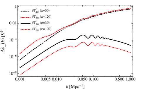
Figure 9: Fluctuations of the gas temperature per logarithmic $k$-interval, at $z=30$ and 120. The two upper lines show the standard result extracted from camb, and the two lower lines show the enhancement resulting from the modulation of small-scale fluctuations by the relative velocity.

IV 21 cm brightness temperature fluctuations during the dark ages

IV.1 Basic equations

The subject of 21 cm absorption and its fluctuations during the dark ages has been treated extensively by multiple authors Loeb and Zaldarriaga (2004); Bharadwaj and Ali (2004); Lewis and Challinor (2007). We are only concerned with computing $(i)$ corrections to the small-scale power spectrum and $(ii)$ the enhancement of large-scale power due to terms quadratic in small-scale fluctuations, which we showed to be uncorrelated with linear terms. We therefore need not concern ourselves with relativistic corrections on large scales, treated in detail in LC07. For completeness, and in order to make all dependencies clear, we briefly summarize the relevant equations below.

IV.1.1 Spin temperature

Following standard conventions, we define the spin temperature $T_{s}$ from the ratio of abundances of neutral hydrogen in the triplet state $n_{1}$ and in the singlet state $n_{0}$ as follows:

$$\frac{n_{1}}{n_{0}}\equiv 3\exp\left(-\frac{E_{10}}{T_{s}}\right)\approx 3\left(1-\frac{E_{10}}{T_{s}}\right),$$ (71)

where $E_{10}\approx 0.068$ K is the energy difference between the two states (corresponding to a transition frequency of 21 cm), and for the second equality we assumed that $T_{s}\gg E_{10}$, which is indeed valid at all times. The spin temperature is determined from a balance between collisional transitions, which tend to set $T_{s}\rightarrow T_{\rm gas}$, and radiative transitions mediated by CMB photons, which tend to set $T_{s}\rightarrow T_{\rm cmb}$.

The rates of upward and downward collisional transitions are denoted by $C_{01}$ and $C_{10}$, respectively, and satisfy the detailed balance relation

$$C_{01}=3\exp\left(-\frac{E_{10}}{T_{\rm gas}}\right)C_{10}\approx 3\left(1-\frac{E_{10}}{T_{\rm gas}}\right)C_{10},$$ (72)

where again we used the fact that $T_{\rm gas}\gg E_{10}$. During the dark ages the Universe is almost fully neutral and collisions with neutral hydrogen atoms largely dominate the collisional transition rate (see Fig. 1 of LC07). The coefficient $C_{10}$ takes the form

$$C_{10}=n_{\rm H}\kappa_{10}^{\rm HH}(T_{\rm gas}),$$ (73)

where the temperature dependence is accurately approximated by the simple fit $\kappa_{10}^{\rm HH}(T_{\rm gas})\approx 3.1\times 10^{-11}T_{\rm gas}^{0.357}\exp(-32/T_{\rm gas})$ cm³ s^-1, with $T_{\rm gas}$ given in Kelvins Kuhlen et al. (2006).

We denote by $R_{10}$ and $R_{01}$ the rates of radiative transitions mediated by CMB photons. The absorption rate $R_{01}$ is related to the rate of spontaneous and stimulated decays $R_{10}$ through the detailed balance relation:

$$R_{01}=3\exp\left(-\frac{E_{10}}{T_{\rm cmb}}\right)R_{10}\approx 3\left(1-\frac{E_{10}}{T_{\rm cmb}}\right)R_{10}.$$ (74)

The latter is given by

$$R_{10}=A_{10}\left(1+\frac{1}{\textrm{e}^{E_{10}/T_{\rm cmb}}-1}\right)\approx A_{10}\frac{T_{\rm cmb}}{E_{10}},$$ (75)

where $A_{10}\approx 2.85\times 10^{-15}$ s^-1 is the spontaneous decay rate. At all times during the dark ages the total transition rate $R_{10}+C_{10}$ surpasses the Hubble rate by several orders of magnitude. The populations of the hyperfine states can therefore be obtained to high accuracy by making the steady-state approximation:

$$n_{1}\left(C_{10}+R_{10}\right)=n_{0}\left(C_{01}+R_{01}\right),$$ (76)

which, using the expressions for the transition rates given above and in the limit $E_{10}\ll T_{\rm gas},T_{\rm cmb}$, leads to the following equation for the spin temperature

$$T_{s}=T_{\rm cmb}+(T_{\rm gas}-T_{\rm cmb})\frac{C_{10}}{C_{10}+A_{10}\frac{T_{\rm gas}}{E_{10}}}.$$ (77)

IV.1.2 Brightness temperature

Following the convention in the field, we define the brightness temperature $T_{b}$ as the temperature characterizing the difference between the radiation field processed by the 21 cm transition and the background CMB radiation field. Since $E_{10}\ll T$ we are in the Rayleigh-Jeans tail of the spectrum. In the optically thin limit, and up to corrections of the order of its peculiar velocity with respect to the CMB Lewis and Challinor (2007), the brightness temperature observed in the gas rest frame is $T_{b}^{\rm local}=\tau\left(T_{s}-T_{\rm cmb}\right)$, where $\tau$ is the Sobolev optical depth, discussed below. The photon phase-space density (or $I_{\nu}/\nu^{3}$ up to multiplicative constants, where $I_{\nu}$ is the specific intensity), is a frame-invariant quantity, conserved in the absence of emission and absorption. This ensures that the ratio $T_{b}/\nu$ is frame-independent and conserved along the photon trajectory. At redshift zero the observed brightness temperature is therefore

$$T_{b}=(1+z)^{-1}\tau\left(T_{s}-T_{\rm cmb}\right),$$ (78)

where again we have neglected corrections of the order of the peculiar velocity of the gas, as well as the effect of gravitational potentials along the photon trajectory. The Sobolev optical depth is given by

$$\tau=\frac{3E_{10}}{32\pi T_{s}}x_{\rm HI}n_{\rm H}\lambda_{10}^{3}\frac{A_{10}}{H+\partial_{\parallel}v_{\parallel}},$$ (79)

where $\lambda_{10}=21$cm, $x_{\rm HI}$ is the fraction of neutral hydrogen and $\partial_{\parallel}v_{\parallel}$ is the line-of-sight gradient (in proper space) of the component of the peculiar velocity along the line of sight. This equation can easily be generalized to arbitrary optical depth by making the replacement $\tau\rightarrow(1-\textrm{e}^{-\tau})$; however, the optical depth is at most a few percent during the dark ages, and we have chosen to keep the lowest-order approximation in order to have more tractable expressions later on.

In the above derivation we have assumed that the line is infinitely narrow. In reality, the line has a finite width due to thermal motions of the atoms (an additional subtlety being that the spin temperature is in fact a velocity-dependent function Hirata and Sigurdson (2007)). This leads to an averaging of fluctuations with radial wavenumber $k_{||}$ larger than $k_{\rm th}\equiv(1+z)^{-1}H\sqrt{m_{\rm H}/T_{\rm gas}}$, which is of the order of the Jeans scale, and is approximately $300$, 400 and 500 Mpc^-1 at $z=100,50$ and 30, respectively. In practice, observations are made with a finite window function, orders of magnitude broader than the thermal line width, and the resulting averaging along the line of sight should dominate any finite line width effects.

In closing of this review section, we point out that the term $\partial_{||}v_{||}$ in the denominator of the optical depth (79) is often referred to as a “redshift-distortion” term. This is a misnomer: although this term is similar to an actual redshift-space distortion term (see Section IV.2.2), it is very different in nature. Redshift-space distortions are an observational effect, they come from the inability of an observer to disentangle the intrinsic cosmological redshift of a source (in a given gauge) from the additional redshifting due to its peculiar velocity along the line of sight. In contrast, the term $\partial_{||}v_{||}$ in the optical depth represents a perturbation of the Hubble expansion rate at the absorber’s location, and does not require any observer (besides the fact that the observer determines the line of sight). It translates the fact that a photon can resonantly interact with less atoms the larger their velocity gradient is along the direction of propagation. See also Ref. Mao et al. (2012).

IV.2 Fluctuations

IV.2.1 Expansion in density and temperature fluctuations

The brightness temperature is a function of the local hydrogen density and gas temperature, and its fluctuations can therefore be expanded in terms of their perturbations. We neglect fluctuations in $T_{\rm cmb}$ and $x_{e}$ and only consider density and temperature fluctuations:

$$n_{\rm H}(z,\boldsymbol{x}) = \overline{n}_{\rm H}(z)\left(1+\delta_{\rm H}(z,\boldsymbol{x})\right),$$ (80)

$$T_{\rm gas}(z,\boldsymbol{x}) = \overline{T}_{\rm gas}(z)\left(1+\delta_{T_{\rm gas}}(z,\boldsymbol{x})\right),$$ (81)

where we recall that $\delta_{\rm H}=\delta_{b}$ up to negligible corrections. We also define the dimensionless small quantity

$$\delta_{v}\equiv\frac{\partial_{\parallel}v_{\parallel}}{H}\equiv\frac{1+z}{H}\nabla_{\parallel}v_{\parallel},$$ (82)

where $\nabla$ is the comoving gradient. The brightness temperature depends locally on $\delta_{v}$ only through $T_{b}\propto(1+\delta_{v})^{-1}$, which will simplify the expression for perturbations.

Combining Eqs. (77) to (79), we expand the brightness temperature to second order in the density and temperature fluctuations.

$$T_{b}=\overline{T}_{b}(1-\delta_{v}+\delta_{v}^{2})+\left(\mathcal{T}_{\rm H}~{}\delta_{\rm H}+\mathcal{T}_{T}~{}\delta_{T_{\rm gas}}\right)(1-\delta_{v})$$

$$+\mathcal{T}_{\rm HH}~{}\delta_{\rm H}^{2}+\mathcal{T}_{{\rm H}T}~{}\delta_{\rm H}\delta_{T_{\rm gas}}+\mathcal{T}_{TT}~{}\delta_{\rm H}^{2}+\mathcal{O}(\delta^{3}),~{}~{}~{}$$ (83)

where the mean brightness temperature is defined by setting all perturbations to zero, and all the coefficients $\mathcal{T}_{ij}$ in the expansion are functions of redshift only.

We have computed the relevant coefficients numerically (see e.g. Ref. Pillepich et al. (2007) for some explicit analytic expressions) and show them in Fig. 10. Their qualitative behavior can be easily understood as follows.

$\bullet$ For $z\gtrsim 100$, collisions efficiently couple the spin temperature to the gas temperature, $T_{s}\approx T_{\rm gas}$. Without the velocity gradient term, we therefore have

$$T_{b}\propto n_{\rm H}\left(1-\frac{T_{\rm cmb}}{T_{\rm gas}}\right).$$ (84)

The dependence on the hydrogen density is linear, so that $\mathcal{T}_{\rm HH}\rightarrow 0$ and $\mathcal{T}_{\rm H}\rightarrow\overline{T}_{\rm b}$. The mean brightness temperature is proportional to $T_{\rm gas}-T_{\rm cmb}$, which becomes closer to zero at high redshift due to efficient Compton heating of the gas by CMB photons. The dependence on $T_{\rm gas}$ in the denominator implies that $\mathcal{T}_{{\rm H}T}\approx\mathcal{T}_{T}\approx-\mathcal{T}_{TT}$, and these functions are not suppressed as $\overline{T}_{b}$ as they do not have a factor of $(T_{\rm gas}-T_{\rm cmb})$: they instead increase at high redshift proportionally to the optical depth $\tau\propto(1+z)^{3/2}$

$\bullet$ For $z\lesssim 50$ collisions become very inefficient and $T_{s}\approx T_{\rm cmb}$, with a small difference proportional to the collision coefficient: $T_{s}-T_{\rm cmb}\propto n_{\rm H}\kappa_{10}(T_{\rm gas}$). This implies that the dependence of the brightness temperature on $n_{\rm H}$ is approximately quadratic so that $\mathcal{T}_{\rm H}\approx 2\overline{T}_{b}\approx 2\mathcal{T}_{\rm HH}$. As time progresses the optical depth gets smaller and all coefficients are rapidly damped.

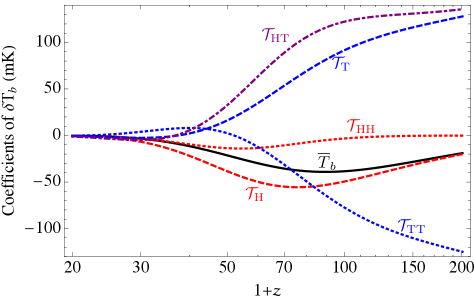
Figure 10: Coefficients of the density and temperature fluctuations in the expansion of the brightness temperature (83), as a function of redshift.

IV.2.2 Redshift-space distortions

In what follows we shall assume that the observer’s peculiar velocity with respect to the CMB can be accurately determined from independent observations, and subtracted.

Let us consider a parcel of absorbing material at redshift $z$, i.e. at comoving radial position

$$r(z)=\int_{0}^{z}\frac{dz^{\prime}}{H(z^{\prime})}.$$ (85)

If the parcel is moving along our line of sight with respect to its local comoving frame with a peculiar velocity $v_{\parallel}$ (where $v_{\parallel}>0$ if the gas is moving away from us), then the observed wavelength of the redshifted 21 cm line is, to first order in $v_{||}$,

$$\lambda_{\rm obs}=\lambda_{10}(1+v_{\parallel})(1+z).$$ (86)

Therefore the observed redshift, which is the only measurable quantity, is given by

$$1+z_{\rm obs}\equiv\frac{\lambda_{\rm obs}}{\lambda_{10}}=(1+z)(1+v_{\parallel}).$$ (87)

From this measured redshift, one would infer a radial comoving distance $r(z_{\rm obs})$, which is related to the actual position $r(z)$ by

$$r(z)\approx r(z_{\rm obs})-\frac{1+z_{\rm obs}}{H(z_{\rm obs})}~{}v_{\parallel}.$$ (88)

The brightness temperature observed at a given wavelength $\lambda_{\rm obs}$ arises from absorption at $r(z)$: $T_{b}^{\rm obs}=T_{b}(r(z))$. Using Eq. (88), and to linear order in $v_{||}$, this is related to $r(z_{\rm obs})$ through

$$T_{b}^{\rm obs}=\left[T_{b}-\frac{1+z}{H}~{}v_{\parallel}\nabla_{\parallel}(\delta T_{b})\right]_{r_{\rm obs}},$$ (89)

where the gradient is with respect to comoving distance along the line of sight (at fixed redshift), and only acts on the perturbation $\delta T_{b}$. This equation and the resulting Fourier transform are equivalent to Eqs. (51) and (56) of Ref. Mao et al. (2012), in the optically thin limit, and to lowest order in $v_{||}$.

The perturbation to the observed brightness temperature is therefore:

$$\delta T_{b}^{\rm obs}=\delta T_{b}(1+\delta_{v})-\frac{1+z}{H}\nabla_{\parallel}(v_{\parallel}\delta T_{b}),$$ (90)

where we have simply used the definition (82) of $\delta_{v}$ and rewritten $\nabla_{\parallel}(v_{\parallel}~{}\delta T_{b})=(\nabla_{\parallel}v_{\parallel})\delta T_{b}+v_{\parallel}\nabla_{\parallel}\delta T_{b}$.

The last term in Eq. (90) is the total derivative of a quadratic term and does not fluctuate on large scales. Indeed, when approximating the spatial average by a statistical average, we have, for any two scalar quantities $\delta_{1},\delta_{2}$,

$$\langle\nabla(\delta_{1}\delta_{2})\rangle = \langle\delta_{1}\nabla\delta_{2}+(\nabla\delta_{1})\delta_{2}\rangle$$ (91)

$$= \int\frac{d^{3}k}{(2\pi)^{3}}\langle\delta_{1}^{*}i\boldsymbol{k}\delta_{2}+(i\boldsymbol{k}\delta_{1})^{*}\delta_{2}\rangle=0.$$

Using Eq. (83) we therefore have, to second order in all fluctuations,

$$\delta T_{b}^{\rm obs} = \mathcal{T}_{\rm H}~{}\delta_{\rm H}+\mathcal{T}_{T}~{}\delta_{T_{\rm gas}}-\overline{T}_{b}~{}\delta_{v}$$

$$+ \mathcal{T}_{\rm HH}\Delta(\delta_{\rm H}^{2})+\mathcal{T}_{TT}\Delta(\delta_{T_{\rm gas}}^{2})+\mathcal{T}_{{\rm H}T}\Delta(\delta_{\rm H}\delta_{T_{\rm gas}}),$$

where $\Delta(\delta_{i}\delta_{j})$ is the fluctuation of the quadratic term $\delta_{i}\delta_{j}$ about its mean value. We see that quadratic terms involving $\delta_{v}$ very conveniently cancel out but emphasize that this is only valid in the optically thin limit; there are additional corrections of order $\tau$ that do contain such terms and that we are neglecting for simplicity.

Following LC07, we define the “monopole source” as:

$$\delta_{s}\equiv\frac{\mathcal{T}_{\rm H}\delta_{\rm H}+\mathcal{T}_{\rm T}\delta_{T_{\rm gas}}^{\rm I}}{\overline{T}_{b}}.$$ (92)

We also define $\delta T_{b}^{\rm II}$ as the total contribution of quadratic terms (and remind the reader that $\delta_{T_{\rm gas}}=\delta_{T_{\rm gas}}^{\rm I}+\delta_{T_{\rm gas}}^{\rm II}$ effectively contains quadratic terms itself):

$$\delta T_{\rm b}^{\rm II} \equiv \mathcal{T}_{\rm HH}\Delta(\delta_{\rm H}^{2})+\mathcal{T}_{TT}\Delta(\delta_{T_{\rm gas}}^{2})$$ (93)

$$+ \mathcal{T}_{{\rm H}T}\Delta(\delta_{\rm H}\delta_{T_{\rm gas}})+\mathcal{T}_{T}~{}\delta_{T_{\rm gas}}^{\rm II}.$$

Finally, we bear in mind that our expression does not account for relativistic corrections on large scales, of order $\sim\overline{T}_{b}\phi,\overline{T}_{b}v$, which we denote by $\delta T_{b}^{\rm rel}$.

Our final expression for the observed brightness temperature is therefore

$$\delta T_{b}^{\rm obs}=\overline{T}_{b}(\delta_{s}-\delta_{v})+\delta T_{b}^{\rm II}+\delta T_{b}^{\rm rel}.$$ (94)

IV.3 Angular power spectrum

We define $P_{0}(k)$ as the power spectrum of the terms independent of the direction of the line of sight, i.e. $\overline{T}_{b}\delta_{s}+\delta T_{b}^{\rm II}+\delta T_{b}^{\rm rel}$. In Fourier space, $\delta_{v}=(\hat{n}\cdot\hat{k})^{2}\theta_{b}/H$, and we define $P_{v}(k)$ as the power spectrum of $\theta_{b}/H$. Finally, we define $P_{0v}(k)$ as the cross-power spectrum of the two.

The angular power spectrum of 21 cm brightness temperature fluctuations from observed redshift $z\equiv z_{\rm obs}\equiv\nu_{21}/\nu_{\rm obs}-1$ is then given by Bharadwaj and Ali (2004); Lewis and Challinor (2007)

$$C_{\ell}(z) = \textrm{e}^{-2\tau_{\rm reion}}\Big{[}4\pi\int\frac{d^{3}k}{(2\pi)^{3}}P_{0}(k,z)\alpha_{\ell}(k,z)^{2}$$ (95)

$$+ 8\pi\int\frac{d^{3}k}{(2\pi)^{3}}P_{0v}(k,z)\alpha_{\ell}(k,z)\beta_{\ell}(k,z)$$

$$+ 4\pi\int\frac{d^{3}k}{(2\pi)^{3}}P_{v}(k,z)\beta_{\ell}(k,z)^{2}\Big{]}$$

where

$$\alpha_{\ell}(k,z) \equiv \int dr^{\prime}j_{\ell}(kr^{\prime})W_{z}(r^{\prime}),$$ (96)

$$\beta_{\ell}(k,z) \equiv \int dr^{\prime}j_{\ell}^{\prime\prime}(kr^{\prime})W_{z}(r^{\prime}),$$ (97)

and $W_{z}(r^{\prime})$ is a window function centered at the radial comoving distance $r(z)$ accounting for the finite spectral resolution $\Delta\nu$. The term $\textrm{e}^{-2\tau_{\rm reion}}$ accounts for Thomson scattering of photons out of the line of sight by free electrons after reionization. In Eq. (95) we have neglected the variation of the various power spectra across the redshift interval $\Delta z$ corresponding to the width of the window function. Since the power spectra vary on a redshift scale $\Delta z\sim z$, this amounts to neglecting terms of order $(\Delta\nu/\nu)^{2}$ provided $\int r^{\prime}W_{z}(r^{\prime})dr^{\prime}=r(z)$.

For $z\gg 1$ and for our fiducial cosmology, $r(z)\approx r(\infty)=14.9$ Gpc. During matter domination, the change in comoving separation corresponding to a frequency width $\Delta\nu/\nu=\Delta z/(1+z)$ is therefore

$$\frac{\Delta r}{r} \approx \frac{c\Delta z}{r(\infty)H_{0}\Omega_{m}^{1/2}(1+z)^{3/2}}\approx\frac{0.57}{\sqrt{1+z}}\frac{\Delta\nu}{\nu}$$ (98)

$$\approx 4\times 10^{-4}\frac{\Delta\nu}{0.1~{}\rm MHz}\sqrt{\frac{1+z}{101}},$$ (99)

where $\nu=1420$ MHz$/(1+z)$ is the observed frequency of the 21 cm transition at redshift $z$. We may use the Limber approximation for $\ell\gg(\Delta r/r)^{-1}$, that is for

$$\ell\gg 2500~{}\frac{0.1~{}\rm MHz}{\Delta\nu}\sqrt{\frac{101}{1+z}}.$$ (100)

In this regime, the velocity terms are suppressed (see Appendix B), and the Limber approximation gives Lewis and Challinor (2007)

$$\frac{\ell^{2}C_{\ell}}{2\pi}\approx\frac{\pi r(z)}{\ell}\frac{k^{3}P_{0}(k)}{2\pi^{2}}\big{|}_{k=\ell/r}\int dr^{\prime}W_{z}(r^{\prime})^{2}.$$ (101)

For scales $\ell\lesssim r/\Delta r$, we compute the angular power spectrum numerically. We first generate the spherical Bessel function up to $\ell=10^{4}$ with sufficient resolution in both $\ell$ and $k$ using a modified version of cmbfast Seljak and Zaldarriaga (1996). We then use a trapezoidal integration scheme to integrate the stored Bessel functions over a Gaussian window function with varying width as prescribed in Eq. (96). We checked for convergence and determined that 200 steps in $r$ are sufficient. In addition we have checked our code for consistency with analytical expressions for a top-hat window function. We also found good agreement with the monopole spectrum generated with camb sources.

IV.3.1 Corrections to the small-scale angular power spectrum

We first consider the small-scale angular power spectrum, $\ell\gtrsim 10^{5}$ corresponding to $k$ greater than a few Mpc^-1. At these scales we only need to consider the terms linear in the baryon density and temperature fluctuations (see Eq. (40) and associated discussion). For definiteness, we shall assume a window function $\Delta\nu=0.1$ MHz and use the Limber approximation, in which the velocity term $\delta_{v}$ cancels. The only relevant term is therefore the “‘monopole” term, which must be averaged over relative velocities.

We show the resulting small-scale power spectrum in Fig. 11 and compare it to the case without relative velocities. We see that the relative velocities lead to power being suppressed by as much as $\sim 50\%$ at the “knee” corresponding to the Jeans scale, $\ell\approx 5\times 10^{6}$. Fluctuations can be enhanced for $\ell\gtrsim 2\times 10^{7}$, due to the resonant excitation of acoustic waves which we described in Section II.3.

Even though the relative velocity affects the small-scale angular power spectrum at order unity, observations of the highly-redshifted 21 cm radiation with an angular resolution $\Delta\theta\lesssim 10^{-5}$ steradian would be extremely challenging, if not merely impossible. We now turn to the still challenging but more accessible large angular scales.

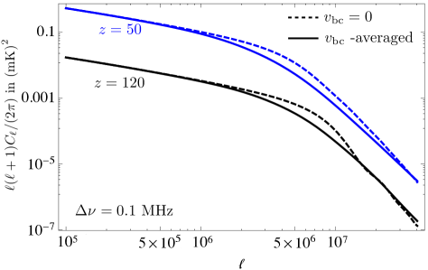
Figure 11: Small-scale angular power spectrum of 21 cm brightness temperature fluctuations at redshifts 120 and 50, neglecting the effect of relative velocities (dashed lines), and averaging over relative velocities (sold lines). The relative change is more than 50% at $\ell\approx 5\times 10^{6}$.

IV.3.2 Corrections to the large-scale angular power spectrum

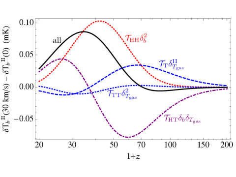
Figure 12: Characteristic amplitude of the quadratic part of 21 cm brightness temperature fluctuations, $\delta T_{b}^{\rm II}(v_{\rm bc}=30$ km/s$)-\delta T_{b}^{\rm II}(0$ km/s), as a function of redshift. The colored lines show the contributions of the different terms, and the black solid line is the sum of them.

Figure 13: Variance of the additional large-scale fluctuation of the 21 cm brightness temperature.

On large angular scales all terms in Eq. (94) are relevant. All terms but the quadratic term were already computed by LC07, and we use the code camb sources to compute them. As we showed earlier, the quadratic terms are uncorrelated with linear terms and we therefore only need to compute the power spectrum of $\delta T_{b}^{\rm II}$, and add it to the LC07 result.

Figure 12 illustrates the redshift dependence of the different terms contributing to $\delta T_{b}^{\rm II}$. We see that they are all of comparable amplitude and happen to nearly cancel out at $z\gtrsim 60$. Figure. 13 shows the variance of the total additional large-scale contribution $\delta T_{b}^{\rm II}$ as a function of redshift. Because of the near-cancellation of the different terms at $z\gtrsim 60$, the fluctuations of the quadratic term peak around $z\approx 30$, at a lower redshift than the fluctuations of the overall 21 cm signal.

Figure 14 shows the power spectrum of $\delta T_{b}^{\rm II}$ compared to the large-scale monopole fluctuations. We see that at $z=30$ the quadratic terms have fluctuations greater than $\sim 10\%$ of those of the monopole term for $k\lesssim 0.01$ Mpc^-1.

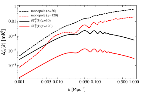
Figure 14: Variance of fluctuations per logarithmic $k$-interval for the quadratic correction (solid) and the standard monopole term (dashed) at $z=30$ (top) and $z=120$ (bottom). The correction is of order tens of percent at large scales and low redshift.

Figure 15 is our main result: it shows the large-scale angular power spectrum $C_{\ell}$ of the quadratic terms, compared with the standard $C_{\ell}$. Because the monopole fluctuation is a rapidly increasing function of $k$, its large-scale angular fluctuations are actually dominated by small-scale power Lewis and Challinor (2007). As a consequence, the correction to the angular power spectrum is smaller than one would expect from comparing the Fourier-space fluctuations. We still find that quadratic terms enhance the large-scale power spectrum by a few percent at $z=30$ and for $\ell$ up to a few hundred. The relative increase is larger when using a larger window function (see right panel of Fig. 15); however in that case the absolute power is also decreased. We note that with the standard cosmological scenario considered, the correction to the large-scale power spectrum is maximal around $z\approx 30$, due to the near-cancellation of various terms at higher redshitfs. One should keep in mind that at these redshifts the radiation from the first stars may alread have a significant impact on the 21 cm signal, depending on the model considered Fialkov et al. (2013b).

Finally, we point out that we have only considered a standard cosmology here, and simply extrapolated the small-scale power spectrum from its known shape at much larger scales. Any unusual feature in the small-scale power spectrum (due, fore example to a running of the spectral index, or to a warm dark matter Loeb and Zaldarriaga (2004)) would also have some effect on large angular scales through the relative velocity effect. This effect therefore potentially allows to measure small-scale physics through observations of large angular scales, an aspect which we shall explore in future works.

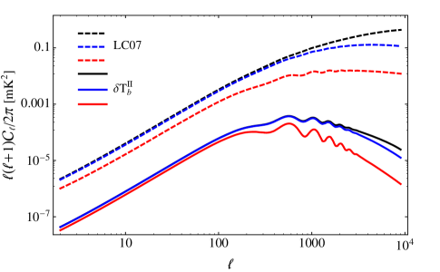
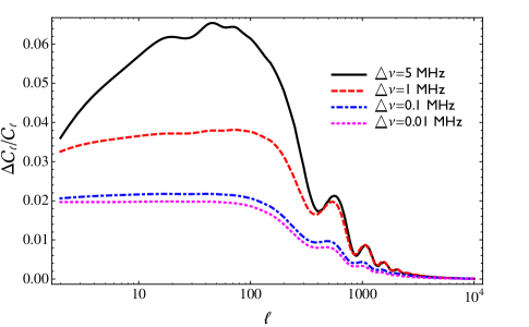
Figure 15: Left: Computed large-scale power spectrum (LC07, including relativistic corrections) and its correction due to the relative velocity between baryons and cold dark matter at redshift 30 and through 3 different windows $\Delta\nu=0.01,0.1$ and $1$ Mhz (top to bottom). Right The relative contribution of the correction at redshift 30. Applying a bigger window transfers more power from large scales, leading to a larger relative contribution.

IV.4 Comment on other non-linear terms

In this paper we are considering quadratic terms only insofar as they are significantly modulated on large scales by the relative velocity. We are neglecting the term $2\langle\delta_{0}\delta_{x}\rangle^{2}$ in the autocorrelation function of $\delta^{2}$, as well as terms of similar order that would result from the correlation of linear terms with cubic terms, $\langle\delta_{0}\delta_{x}^{3}\rangle=3\langle\delta^{2}\rangle\langle\delta_{0}\delta_{x}\rangle$. This neglect is formally justified, since our correction to the simple linear analysis at large scales is of relative order $(\delta_{s}^{2}/\delta_{l})^{2}\sim 1$, whereas other non-linear terms are formally corrections of order $\delta^{2}\ll 1$. In practice, however, our large-scale correction is numerically of the order of tens of percent, and is the largest at $z\sim 30$. By then the variance of the density fluctuation is already several percent, and the neglected non-linear terms could therefore be of comparable magnitude as the one we have accounted for, even though they are formally of a different order. To our knowledge, the effect of higher-order terms in the brightness temperature expansion has not been investigated yet (beside Ref. Shaw and Lewis (2008), where the non-linear velocity gradient terms are considered, see also Ref. Mao et al. (2012)). Including the other non-linear terms consistently would also require accounting for the non-linear growth of overdensities. This would significantly complicate the analysis, and we defer it to a future work.

V Conclusions

We have revisited the theoretical prediction for the 21 cm intensity fluctuations during the dark ages, accounting for the relative velocity between baryons and CDM recently discussed by Tseliakhovich and Hirata Tseliakhovich and Hirata (2010). We have focused on isolating the consequences of this effect and for the sake of simplicity have made several assumptions regarding other effects which can be important at the few-percent level. Some of these effects are treated elsewhere in the literature and we list them here for completeness. First, we have computed the signal to lowest order in the small optical depth and neglected fluctuations of the residual free electron fraction, which lead to a few percent correction Lewis and Challinor (2007). This can be straightforwardly accounted for in our computation, and we have not done so simply for the sake of conciseness. Secondly, we have neglected the thermal broadening of the 21 cm line and have assumed it can be described by a single, velocity-independent spin temperature, effects which can be important at the percent-level Hirata and Sigurdson (2007). Finally, we have used linear perturbation theory to follow the growth of density perturbations, and neglected non-linear corrections which affect the small-scale power spectrum at the several percent level at $z\lesssim 50$. Computing these corrections accurately is technically challenging and has only been done approximately so far Lewis and Challinor (2007). We have also neglected higher-order terms in the expansion of the brightness temperature, which could lead to corrections at the several percent level at low redshift. To our knowledge, these corrections have not yet been explored. Last but not least, we have neglected the impact that early-formed stars may have on the signal at $z\approx 30$.

Our findings are as follows. The relative velocity between baryons and CDM leads to a suppression of baryonic density and temperature fluctuations on scales $k\gtrsim 30$ Mpc^-1 by several tens of percent, which result in a similar suppression of the 21 cm fluctuations on angular scales $\ell\gtrsim 5\times 10^{5}$. Less intuitively, we find an enhancement of the 21 cm fluctuations in two scale regimes. First, on scales much smaller than the Jeans scale, we find that the streaming of cold dark matter perturbations relative to baryonic ones lead to a resonant amplification of acoustic waves. This translates to an enhancement of the 21 cm power spectrum for angular scales $\ell\gtrsim 5\times 10^{7}$. Most importantly (and as anticipated by TH10), the large-scale fluctuations of the relative velocity field are imprinted on the 21 cm signal, at scales $k\sim 0.005-1$ Mpc^-1, corresponding to angular scales $\ell\lesssim 10^{4}$. This enhancement is due to the combination of two facts. On the one hand, the 21 cm brightness temperature depends non-linearly on the underlying baryonic fluctuations. On the other hand, the large-scale modulation by the relative velocity of the square of small-scale perturbations is comparable to the linear large-scale fluctuations at $z\lesssim 100$.

One of the prime appeals of 21 cm fluctuations from the dark ages is to access the small-scale power spectrum at $k\gtrsim$ few Mpc^-1, currently unaccessible to other probes Loeb and Zaldarriaga (2004); Tegmark and Zaldarriaga (2009). If observed directly, these Fourier modes correspond to multipoles $\ell$ of several tens of thousands at least, i.e. an angular resolution better than $10^{-4}$ radians. Reaching this resolution at the highly redshifted frequency of the 21 cm transition would be highly challenging, requiring very large baselines. Our results show that detection prospects are in fact more optimistic (though still challenging): the relative velocity imprints the characteristic amplitude of the small-scale density power spectrum (around $k\sim 100$ Mpc^-1) on large angular fluctuations of the 21 cm signal, around $\ell\lesssim 1000$. Note that the relative velocity perturbations have support on scales which are well measured by current cosmological probes, and can therefore be computed exactly. Any deviation from the standard cosmological model on small scales, such as warm dark matter or a running of the primordial power spectrum, would therefore not only affect the small angular scales of 21 cm fluctuations, but also the regime $\ell\lesssim 1000$. The relative velocity should also significantly change the effect that dark matter annihilations would have on the 21 cm signal fluctuations Natarajan and Schwarz (2009). We plan to investigate these issues in future work.

Another extension to the work presented here is to include effects of primordial non-Gaussianity; similarly to the relative velocity, non-Gaussianities modulate the small-scale power spectrum on large scales in the squeezed limit. It is interesting to know how these effects compare, both as a function of scale as well as amplitude, and whether the relative velocity may hamper or help detection of primordial non-gaussianities with 21 cm fluctuations.

Finally, the analytical results presented here also encourage to look for semi-analytical modeling of the low redshift Universe. So far, this has predominantly been a numerical effort, but it is not unlikely that some of the physics at late times can be modeled analytically. We shall tackle this problem in future work.

Appendix A Autocorrelation of functions of the relative velocity

In Section IV we had to compute the autocorrelation function of the form $\langle F(v_{0})F(v_{x})\rangle$ of terms quadratic in small-scale fluctuations which depend on the magnitude of the local relative velocity (for which we have dropped the subscript bc). In this Appendix we describe our numerical method and derive analytical approximations for the two limiting cases of weak and strong correlation.

This autocorrelation takes the following integral form:

$$\langle F(v_{0})F(v_{x})\rangle\equiv\int d^{3}\boldsymbol{u}_{\boldsymbol{0}}~{}d^{3}\boldsymbol{u}_{\boldsymbol{x}}P(\boldsymbol{u}_{\boldsymbol{0}},\boldsymbol{u}_{\boldsymbol{x}})F(\sigma_{1d}u_{0})F(\sigma_{1d}u_{x}),~{}~{}~{}~{}$$ (102)

where $P(\boldsymbol{u}_{\boldsymbol{0}},\boldsymbol{u}_{\boldsymbol{x}})$ is the six-dimensional joint Gaussian probability distribution for the normalized relative velocities $\boldsymbol{u}_{0}\equiv\boldsymbol{v}_{0}/\sigma_{1d},\boldsymbol{u}_{x}\equiv\boldsymbol{v}_{x}/\sigma_{1d}$, at two points separated by comoving distance $\boldsymbol{x}$:

$$P(\boldsymbol{u}_{\boldsymbol{0}},\boldsymbol{u}_{\boldsymbol{x}})=\frac{1}{(2\pi)^{3}\sqrt{1-c_{||}^{2}}(1-c_{\bot}^{2})}\exp\left[-\frac{1}{2}\frac{u_{0||}^{2}+u_{x||}^{2}-2c_{||}u_{0||}u_{x||}}{1-c_{||}^{2}}-\frac{1}{2}\frac{\boldsymbol{u}_{0\bot}^{2}+\boldsymbol{u}_{x\bot}^{2}-2c_{\bot}\boldsymbol{u}_{0\bot}\cdot\boldsymbol{u}_{x\bot}}{1-c_{\bot}^{2}}\right],$$ (103)

where $\boldsymbol{u}_{||}=\boldsymbol{u}\cdot\hat{x}$, $\boldsymbol{u}_{\bot}=\boldsymbol{u}-u_{||}\hat{x}$, and the dimensionless correlation coefficients $c_{||}(x),c_{\bot}(x)$ were defined in Eq. (5).

A.1 General case

When the correlation coefficients are neither small nor very close to unity, we have to compute the integral (102) numerically. Using spherical polar coordinates with $\hat{x}$ as the polar axis, one of the angular integrals is trivial, and the other can be performed analytically, so that the remaining integral is only four-dimensional, and takes the form Dalal et al. (2010):

$$\langle F(v_{0})F(v_{x})\rangle=\iint_{0}^{\infty}du_{0}du_{x}F(\sigma_{1d}u_{0})F(\sigma_{1d}u_{x})\mathcal{P}(u_{0},u_{x}),$$ (104)

where the joint probability distribution for the normalized magnitudes is given by

$$\mathcal{P}(u_{0},u_{x})\equiv\frac{u_{0}^{2}u_{x}^{2}}{2\pi\sqrt{1-c_{||}^{2}}(1-c_{\bot}^{2})}\iint_{-1}^{1}d\mu_{0}d\mu_{x}\exp\left[-\frac{1}{2}\frac{u_{0||}^{2}+u_{x||}^{2}-2c_{||}u_{0||}u_{x||}}{1-c_{||}^{2}}-\frac{1}{2}\frac{u_{0\bot}^{2}+u_{x\bot}^{2}}{1-c_{\bot}^{2}}\right]\mathcal{I}_{0}\left[\frac{c_{\bot}u_{0\bot}u_{x\bot}}{1-c_{\bot}^{2}}\right],~{}~{}~{}~{}~{}$$ (105)

where $u_{0||}\equiv u_{0}\mu_{0},u_{0\bot}\equiv u_{0}\sqrt{1-\mu_{0}^{2}}$ and similarly for $u_{x||},u_{x\bot}$, and $\mathcal{I}_{0}$ is the zero-th order modified Bessel function of the first kind.

In order to speed up computations, we first pre-compute the redshift-independent distribution $\mathcal{P}(u_{0},u_{x})$ as a function of $u_{0},u_{x}$ and the magnitude $x$ of the separation vector. We can then quickly compute the remaining two-dimensional integral for any given specific function $F$, in particular for the same physical quantity at different redshifts.

A.2 Small separation, strong correlation limit

When $x\rightarrow 0$, $c_{\parallel},c_{\bot}\rightarrow 1$ and the joint probability distribution $P(\boldsymbol{u}_{0},\boldsymbol{u}_{x})$ becomes sharply peaked around $\boldsymbol{u}_{x}=\boldsymbol{u}_{0}$, which makes direct numerical integration difficult. In this section we derive an asymptotic expression valid in this regime. We start by rewriting

$$P(\boldsymbol{u}_{0},\boldsymbol{u}_{x})=P(\boldsymbol{u_{0}})\prod_{i}P(u_{x}^{i}|u_{0}^{i}),$$ (106)

where $P(\boldsymbol{u}_{0})$ is an isotropic three-dimensional Gaussian distribution with unit variance per axis and $P(u_{x}^{i}|u_{0}^{i})$ is a one-dimensional Gaussian distribution with mean $c_{i}u_{0}^{i}$ and variance $1-c_{i}^{2}$, with $c_{1}=c_{||}$ and $c_{2}=c_{3}=c_{\bot}$. We now Taylor-expand $\tilde{F}(u_{x})\equiv F(\sigma_{1d}u_{x})$ around $\boldsymbol{u}_{0}$. In order to get a correct expression at order $\mathcal{O}(1-c_{i})$ we need to carry the expansion to second order in $\Delta^{i}\equiv u_{x}^{i}-u_{0}^{i}$. Dropping the tilde on $F$, we have:

$$F(u_{x})\approx F(u_{0})+\sum_{i}\Delta^{i}\partial_{i}F+\frac{1}{2}\sum_{ij}\Delta^{i}\Delta^{j}\partial_{i}\partial_{j}F+\mathcal{O}(\Delta^{3}).$$ (107)

We integrate this expression over the constrained distribution of $u_{x}^{i}$ and obtain, to order $1-c_{i}$:

$$\langle\Delta^{i}\rangle = -(1-c_{i})u_{0}^{i},$$ (108)

$$\langle\Delta^{i}\Delta^{j}\rangle = \delta^{ij}(1-c_{i}^{2})+(1-c_{i})(1-c_{j})u_{0}^{i}u_{0}^{j}\approx 2\delta^{ij}(1-c_{i}).$$ (109)

We therefore obtain

$$\langle F(u_{0})F(u_{x})\rangle \approx \langle F(u_{0})^{2}\rangle+\sum_{i}(1-c_{i})\left[\langle F\partial_{i}^{2}F\rangle-\langle u_{0}^{i}F\partial_{i}F\rangle\right]+\mathcal{O}(1-c_{i})^{2},$$ (110)

where the argument $u_{0}$ is implicit everywhere. We now recall that the Gaussian probability distribution $P(\boldsymbol{u}_{0})$ satisfies the differential equation $\partial_{i}P=-u_{0}^{i}P$, which, after integration by parts, leads to the identity $\langle u_{0}^{i}G\rangle=\langle\partial_{i}G\rangle$ for any function $G$. This allows us to simplify equation (110):

$$\langle F(u_{0})F(u_{x})\rangle\approx\langle F^{2}\rangle-\sum_{i}(1-c_{i})\langle(\partial_{i}F)^{2}\rangle+\mathcal{O}(1-c_{i})^{2}.$$ (111)

From the isotropy of $F$ and $P$ we have $\langle(\partial_{i}F)^{2}\rangle=\frac{1}{3}\langle(\nabla F)^{2}\rangle=\frac{1}{3}\langle(F^{\prime})^{2}\rangle$. We therefore arrive at the following expression, valid in the small-separation limit:

$$\langle F(u_{0})F(u_{x})\rangle\approx\langle F^{2}\rangle-(1-\overline{c})\langle(F^{\prime})^{2}\rangle,$$ (112)

where $\overline{c}\equiv\frac{1}{3}c_{||}+\frac{2}{3}c_{\bot}$ is the spherically-averaged correlation coefficient.

It is in principle straightforward to carry on this expansion to higher order in $(1-c_{i})$. However, the resulting coefficients depend on higher-order derivatives of $F$, which is itself a numerically evaluated function, and whose numerical higher-order derivatives are less and less accurate. We have therefore chosen to stop at the first order given here. In practice we use this expansion for $x\leq 3$ Mpc, for which $1-\overline{c}\leq 0.03$, and switch to numerical integration beyond that value.

A.3 Large separation, weak correlation limit

In the other limiting regime, $x\rightarrow\infty$, $c_{i}\rightarrow 0$, the autocorrelation of the mean-subtracted function $F$ becomes vanishingly small. Direct numerical integration cannot properly capture the near-vanishing of the integral, and here also we may use a series expansion. We expand the probability distribution $P(\boldsymbol{u}_{0},\boldsymbol{u}_{x})$ to second order in $c_{i}\ll 1$:

$$P(\boldsymbol{u}_{0},\boldsymbol{u}_{x})=\frac{\exp\left[-\frac{1}{2}\sum_{i}\frac{u_{0i}^{2}+u_{xi}^{2}}{1-c_{i}^{2}}\right]}{(2\pi)^{3}\sqrt{1-c_{||}^{2}}(1-c_{\bot}^{2})}\left(1+\sum_{i}\frac{c_{i}u_{0i}u_{xi}}{1-c_{i}^{2}}+\frac{1}{2}\sum_{ij}c_{i}c_{j}u_{0i}u_{xi}u_{0j}u_{xj}+\mathcal{O}(c_{i}^{3})\right).$$ (113)

Since the function $F$ only depends on the magnitude of $\boldsymbol{u}$, it is an even function of the $u_{i}$. Therefore upon integration against $F(u_{0})F(u_{x})$, only the term $c_{i}^{2}u_{0i}^{2}u_{xi}^{2}$ survives, and to lowest order we get

$$\langle F(u_{0})F(u_{x})\rangle\approx\frac{1}{2}\sum_{i}c_{i}^{2}\langle u_{i}^{2}F(u)\rangle^{2}=\frac{1}{18}\langle u^{2}F(u)\rangle^{2}\sum_{i}c_{i}^{2},$$ (114)

where the radial averaging is to be carried with an isotropic Gaussian distribution, and we recall that $\langle F\rangle=0$. In practice, we use this approximation for $\sum_{i}c_{i}^{2}\leq 10^{-4}$.

As an example, we show the autocorrelation function of $\delta_{b}^{2}$ and the resulting power spectrum obtained by Fourier transforming it in Fig. 16, where we compare it to the power spectrum of the linear overdensity. We see that the power spectrum of $\delta_{b}^{2}$ can be comparable to that of $\delta_{b}$ on very large scales ($k\lesssim 0.01$ Mpc^-1) and at low redshifts. For $z=30$, the ratio of power spectra is greater than 10 percent for $k\lesssim 0.1$ Mpc^-1. Even at $z=120$, the ratio is still of order a percent or more on scales $k\lesssim 0.01$ Mpc^-1.

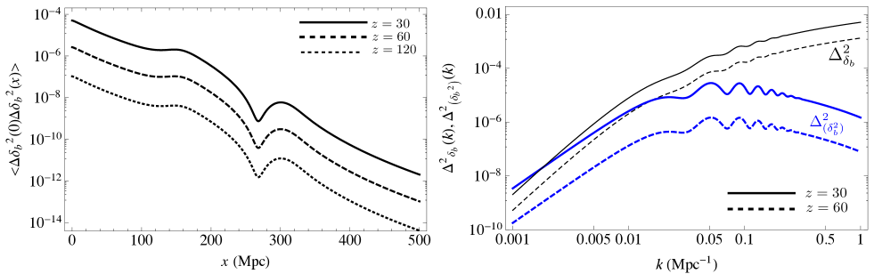
Figure 16: Left: Autocorrelation function of the fluctuations of $\delta_{b}^{2}$ due to the modulation of small-scale power by the relative velocity of baryons and CDM. Right: Variance of fluctuations of the baryon overdensity (thin black lines) and of its square (thick blue lines) per logarithmic $k$-interval, at $z=60$ and 30. The large-scale power spectrum of $\delta_{b}$ is computed with camb in the synchronous gauge. We only show scales inside the horizon for which the overdensity is not strongly dependent on the chosen gauge.

Appendix B Analytic expressions for the angular power spectrum for $\Delta^{2}(k)\propto k$.

In this section we give analytic expressions for the angular power spectrum, valid for all $\ell\gg 1$ and all widths of observational window function $\Delta\equiv\Delta r/r\ll 1$, if the underlying three-dimensional power spectra grow as $\Delta^{2}(k)\propto k$. The suppression factor $\textrm{e}^{-2\tau_{\rm reion}}$ is implicit everywhere.

The angular power spectrum at redshift $z$ takes the form $C_{\ell}(z)\equiv C_{\ell}^{0}+C_{\ell}^{0v}+C_{\ell}^{v}$, where the three components are given in Eq. (95). In this section we shall derive analytic expressions in the case where $\Delta_{0}^{2}(k)\equiv k^{3}P_{0}(k)/(2\pi^{2})\propto k$, and similarly for $\Delta_{0v}^{2}$ and $\Delta_{v}^{2}$.

With this assumption on the scale dependence, the first term is

$$C_{\ell}^{0}=4\pi\Delta_{0}^{2}(\ell/r_{z})\frac{r_{z}}{\ell}\int dr_{1}dr_{2}W_{z}(r_{1})W_{z}(r_{2})\frac{1}{r_{1}}\int dxj_{\ell}(x)j_{\ell}\left((r_{2}/r_{1})x\right).$$ (115)

This integral involves the function

$$F_{\ell}(R)\equiv\int dxj_{\ell}(x)j_{\ell}(Rx).$$ (116)

Using the differential equation satisfied by the spherical Bessel functions, we obtain the following differential equation for $F_{\ell}(R)$:

$$R^{2}F_{\ell}^{\prime\prime}+2RF_{\ell}^{\prime}-\ell(\ell+1)F_{\ell}=-R^{2}\int dx~{}x^{2}j_{\ell}(x)j_{\ell}(Rx)=-\frac{\pi}{2}\delta(R-1),$$ (117)

where in the second equality we have used the orthogonality relation for the spherical Bessel functions. The homogeneous solutions of this equation are $F_{\ell}(R)\propto R^{\ell}$ and $F_{\ell}(R)\propto R^{-(\ell+1)}$. Integrating the ODE with initial condition $F_{\ell}(0)=0$, requiring continuity of $F_{\ell}$ at $R=1$ and the jump condition for its derivative $F_{\ell}^{\prime}(1^{+})-F_{\ell}^{\prime}(1^{-})=-\pi/2$, we arrive at

$$F_{\ell}(R)\ =\begin{dcases}\frac{\pi R^{\ell}}{2(2\ell+1)}&\text{if }R\leq 1\\ \frac{\pi R^{-(\ell+1)}}{2(2\ell+1)}&\text{if }R\geq 1\\ \end{dcases}\approx\frac{\pi}{4\ell}\textrm{e}^{-\ell|R-1|}\ \ \text{if}\ |R-1|\ll 1\ \text{and}\ \ \ell\gg 1,$$ (118)

where the limit is valid for either sign of $R-1$. We rewrite Eq. (115) with $r_{1}=r_{z}(1+\epsilon_{1})$ and $r_{2}=r_{z}(1+\epsilon_{2})$. For a top-hat window function the outer integral becomes, to lowest order in $\epsilon_{1},\epsilon_{2}$

$$C_{\ell}^{0}\approx\frac{\pi^{2}}{\ell^{2}}\Delta_{0}^{2}(\ell/r_{z})\frac{1}{\Delta^{2}}\iint_{-\Delta/2}^{\Delta/2}d\epsilon_{1}d\epsilon_{2}~{}\textrm{e}^{-\ell|\epsilon_{2}-\epsilon_{1}|}=\frac{\pi^{2}}{\ell^{2}}\Delta_{0}^{2}(\ell/r_{z})\frac{2(\ell\Delta-1+\textrm{e}^{-\ell\Delta})}{(\ell\Delta)^{2}}.$$ (119)

We therefore obtain the following general expression and asymptotic limits:

$$\frac{\ell^{2}}{2\pi}C_{\ell}^{0}\approx\frac{\pi}{2}\Delta_{0}^{2}(\ell/r_{z})\frac{2(\ell\Delta-1+\textrm{e}^{-\ell\Delta})}{(\ell\Delta)^{2}}\approx\begin{dcases}\frac{\pi}{2}\Delta_{0}^{2}(\ell/r_{z})&\text{if}\ \ \ell\Delta\ll 1,\\ \frac{\pi}{\ell\Delta}\Delta_{0}^{2}(\ell/r_{z})&\text{if}\ \ \ell\Delta\gg 1.\end{dcases}$$ (120)

Next we consider the cross term. We need to compute the function

$$G_{\ell}(R)\equiv\int dxj_{\ell}(x)j_{\ell}^{\prime\prime}(Rx)=\frac{d^{2}}{dR^{2}}\int\frac{dx}{x^{2}}j_{\ell}(x)j_{\ell}(Rx)\equiv\frac{d^{2}}{dR^{2}}H_{\ell}(R),$$ (121)

where the second equality is valid for $R\neq 1$ and the last one defines the function $H_{\ell}$. Using again the differential equation satisfied by $j_{\ell}$, we obtain the following equation for $H_{\ell}(R)$:

$$R^{2}H_{\ell}^{\prime\prime}+2RH_{\ell}^{\prime}-\ell(\ell+1)H_{\ell}=-R^{2}F_{\ell},$$ (122)

from which we get the following equation for $G_{\ell}=H_{\ell}^{\prime\prime}$:

$$R^{2}G_{\ell}^{\prime\prime}+6RG_{\ell}^{\prime}+\left(6-\ell(\ell+1)\right)G_{\ell}=-\frac{d^{2}}{dR^{2}}(R^{2}F_{\ell}).$$ (123)

One can obtain an explicit solution given the boundary conditions $G_{\ell}(0)=G_{\ell}(\infty)=0$ and requiring that $G_{\ell}$ is continuous at $R=1$. In the limit $|R-1|\ll 1,\ell\gg 1$ of interest, we obtain

$$G_{\ell}(R)\approx-\frac{\pi}{8\ell}\textrm{e}^{-\ell|R-1|}(1-\ell|R-1|),$$ (124)

and as a consequence,

$$C_{\ell}^{0v}\approx-\frac{\pi^{2}}{\ell^{2}}\Delta_{0v}^{2}(\ell/r_{z})\frac{1}{\Delta^{2}}\iint_{-\Delta/2}^{\Delta/2}d\epsilon_{1}d\epsilon_{2}\textrm{e}^{-\ell|\epsilon_{2}-\epsilon_{1}|}(1-\ell|\epsilon_{2}-\epsilon_{1}|)=-\frac{\pi^{2}}{\ell^{2}}\Delta_{0v}^{2}(\ell/r_{z})\frac{2(1-\textrm{e}^{-\ell\Delta}(1+\ell\Delta))}{(\ell\Delta)^{2}}.$$ (125)

We therefore arrive at the following general expression and corresponding asymptotic regimes for the cross term:

$$\frac{\ell^{2}}{2\pi}C_{\ell}^{0v}\approx-\frac{\pi}{2}\Delta_{0v}^{2}(\ell/r_{z})\frac{2(1-\textrm{e}^{-\ell\Delta}(1+\ell\Delta))}{(\ell\Delta)^{2}}\approx\begin{dcases}-\frac{\pi}{2}\Delta_{0v}^{2}(\ell/r_{z})&\text{if}\ \ \ell\Delta\ll 1,\\ -\frac{\pi}{(\ell\Delta)^{2}}\Delta_{0v}^{2}(\ell/r_{z})&\text{if}\ \ \ell\Delta\gg 1,\end{dcases}$$ (126)

We compute the power spectrum of the velocity term with similar techniques, and arrive at

$$\frac{\ell^{2}}{2\pi}C_{\ell}^{v}\approx\frac{\pi}{8}\Delta_{v}^{2}(\ell/r_{z})\frac{1-\textrm{e}^{-\ell\Delta}(1+\ell\Delta-\ell^{2}\Delta^{2})}{(\Delta\ell)^{2}}\approx\begin{dcases}\frac{3\pi}{16}\Delta_{v}^{2}(\ell/r_{z})&\text{if}\ \ \ell\Delta\ll 1,\\ \frac{\pi}{8(\ell\Delta)^{2}}\Delta_{v}^{2}(\ell/r_{z})&\text{if}\ \ \ell\Delta\gg 1,\end{dcases}$$ (127)

To conclude, we find, for power spectra scaling as $\Delta^{2}(k)\propto k$ (i.e. for equal power per linear $k$-interval), that, in the narrow window regime, we get

$$\frac{\ell^{2}}{2\pi}C_{\ell}\approx\frac{\pi}{2}\Delta_{0}^{2}(\ell r_{z})-\frac{\pi}{2}\Delta_{0v}^{2}(\ell r_{z})+\frac{3\pi}{16}\Delta_{v}^{2}(\ell r_{z}),\ \ \text{for}\ \ell\Delta\ll 1,$$ (128)

which agrees with equation (41) of LC07. In the large-window function regime, the terms involving velocities along the line of sight are suppressed by $1/(\ell\Delta r/r)^{2}$, whereas the “monopole” term is only suppressed by $1/(\ell\Delta r/r)$ and therefore dominates the angular power spectrum:

$$\frac{\ell^{2}}{2\pi}C_{\ell}\approx\frac{\pi}{\ell\Delta}\Delta_{0}^{2}(\ell/r_{z}),\ \ \text{for}\ \ell\Delta\gg 1,$$ (129)

in agreement with equation (43) of LC07. This appendix moreover provides explicit forms for the transition regime valid for $\Delta^{2}(k)\propto k$.

References

- Furlanetto et al. (2006) S. R. Furlanetto, S. P. Oh, and F. H. Briggs, Phys. Rep. 433, 181 (2006), arXiv:astro-ph/0608032 .
- Pritchard and Loeb (2008) J. R. Pritchard and A. Loeb, Phys. Rev. D 78, 103511 (2008), arXiv:0802.2102 .
- Furlanetto et al. (2009) S. R. Furlanetto et al., in astro2010: The Astronomy and Astrophysics Decadal Survey, ArXiv Astrophysics e-prints, Vol. 2010 (2009) p. 82, arXiv:0902.3259 [astro-ph.CO] .
- Loeb and Zaldarriaga (2004) A. Loeb and M. Zaldarriaga, Physical Review Letters 92, 211301 (2004), arXiv:astro-ph/0312134 .
- Mao et al. (2008) Y. Mao, M. Tegmark, M. McQuinn, M. Zaldarriaga, and O. Zahn, Phys.Rev. D78, 023529 (2008), arXiv:0802.1710 [astro-ph] .
- Lewis and Challinor (2007) A. Lewis and A. Challinor, Phys. Rev. D 76, 083005 (2007), arXiv:astro-ph/0702600 [LC07] .
- Bharadwaj and Ali (2004) S. Bharadwaj and S. S. Ali, Mon. Not. R. Astron. Soc. 352, 142 (2004), arXiv:astro-ph/0401206 .
- Tseliakhovich and Hirata (2010) D. Tseliakhovich and C. Hirata, Phys. Rev. D 82, 083520 (2010).
- Tseliakhovich et al. (2011) D. Tseliakhovich, R. Barkana, and C. M. Hirata, Mon. Not. R. Astron. Soc. 418, 906 (2011).
- Bittner and Loeb (2011) J. M. Bittner and A. Loeb, ArXiv e-prints (2011), arXiv:1110.4659 [astro-ph.CO] .
- Fialkov et al. (2012) A. Fialkov, R. Barkana, D. Tseliakhovich, and C. M. Hirata, Mon. Not. R. Astron. Soc. 424, 1335 (2012), arXiv:1110.2111 [astro-ph.CO] .
- Visbal et al. (2012) E. Visbal, R. Barkana, A. Fialkov, D. Tseliakhovich, and C. M. Hirata, Nature (London) 487, 70 (2012), arXiv:1201.1005 [astro-ph.CO] .
- Fialkov et al. (2013a) A. Fialkov, R. Barkana, E. Visbal, D. Tseliakhovich, and C. M. Hirata, Mon. Not. R. Astron. Soc. 432, 2909 (2013a), arXiv:1212.0513 [astro-ph.CO] .
- Fialkov et al. (2013b) A. Fialkov, R. Barkana, A. Pinhas, and E. Visbal, ArXiv e-prints (2013b), arXiv:1306.2354 [astro-ph.CO] .
- Wouthuysen (1952) S. A. Wouthuysen, Astron. J. 57, 31 (1952).
- Field (1958) G. B. Field, Proceedings of the IRE 46, 240 (1958).
- Hirata (2006) C. M. Hirata, Mon. Not. R. Astron. Soc. 367, 259 (2006), arXiv:astro-ph/0507102 .
- Carilli et al. (2007) C. L. Carilli, J. N. Hewitt, and A. Loeb, ArXiv Astrophysics e-prints (2007), arXiv:astro-ph/0702070 .
- Planck Collaboration et al. (2013) Planck Collaboration, P. A. R. Ade, N. Aghanim, C. Armitage-Caplan, M. Arnaud, M. Ashdown, F. Atrio-Barandela, J. Aumont, C. Baccigalupi, A. J. Banday, and et al., ArXiv e-prints (2013), arXiv:1303.5076 [astro-ph.CO] .
- Eisenstein and Hu (1998) D. J. Eisenstein and W. Hu, Astrophys. J. 496, 605 (1998), arXiv:astro-ph/9709112 .
- Dalal et al. (2010) N. Dalal, U.-L. Pen, and U. Seljak, J. Cosm. Astropart. Phys. 11, 007 (2010), arXiv:1009.4704 [astro-ph.CO] .
- Lewis et al. (2000) A. Lewis, A. Challinor, and A. Lasenby, Astrophys.J. 538, 473 (2000), arXiv:astro-ph/9911177 [astro-ph] .
- Bernardeau et al. (2012) F. Bernardeau, N. van de Rijt, and F. Vernizzi, Phys. Rev. D 85, 063509 (2012), arXiv:1109.3400 [astro-ph.CO] .
- Bernardeau et al. (2013) F. Bernardeau, N. Van de Rijt, and F. Vernizzi, Phys. Rev. D 87, 043530 (2013), arXiv:1209.3662 [astro-ph.CO] .
- Ma and Bertschinger (1995) C.-P. Ma and E. Bertschinger, Astrophys. J. 455, 7 (1995), arXiv:astro-ph/9506072 .
- Naoz and Barkana (2005) S. Naoz and R. Barkana, Mon. Not. R. Astron. Soc. 362, 1047 (2005), arXiv:astro-ph/0503196 .
- Switzer and Hirata (2008) E. R. Switzer and C. M. Hirata, Phys. Rev. D 77, 083006 (2008), arXiv:astro-ph/0702143 .
- Seager et al. (2000) S. Seager, D. D. Sasselov, and D. Scott, Astrophys. J. Suppl. Ser. 128, 407 (2000), arXiv:astro-ph/9912182 .
- Senatore et al. (2009) L. Senatore, S. Tassev, and M. Zaldarriaga, J. Cosm. Astropart. Phys. 8, 031 (2009), arXiv:0812.3652 .
- Pillepich et al. (2007) A. Pillepich, C. Porciani, and S. Matarrese, Astrophys. J. 662, 1 (2007), astro-ph/0611126 .
- Chen and Kamionkowski (2004) X. Chen and M. Kamionkowski, Phys. Rev. D 70, 043502 (2004), astro-ph/0310473 .
- Giesen et al. (2012) G. Giesen, J. Lesgourgues, B. Audren, and Y. Ali-Haïmoud, J. Cosm. Astropart. Phys. 12, 008 (2012), arXiv:1209.0247 [astro-ph.CO] .
- Dvorkin et al. (2013) C. Dvorkin, K. Blum, and M. Zaldarriaga, Phys. Rev. D 87, 103522 (2013), arXiv:1302.4753 [astro-ph.CO] .
- Ali-Haïmoud and Hirata (2011) Y. Ali-Haïmoud and C. M. Hirata, Phys. Rev. D 83, 043513 (2011), arXiv:1011.3758 [astro-ph.CO] .
- Hirata and Forbes (2009) C. M. Hirata and J. Forbes, Phys. Rev. D 80, 023001 (2009), arXiv:0903.4925 [astro-ph.CO] .
- Chluba and Sunyaev (2010) J. Chluba and R. A. Sunyaev, Astron. Astrophys. 512, A53 (2010), arXiv:0904.0460 [astro-ph.CO] .
- Peebles (1968) P. J. E. Peebles, Astrophys. J. 153, 1 (1968).
- Zel’dovich et al. (1969) Y. B. Zel’dovich, V. G. Kurt, and R. A. Syunyaev, Soviet Journal of Experimental and Theoretical Physics 28, 146 (1969).
- Pequignot et al. (1991) D. Pequignot, P. Petitjean, and C. Boisson, Astron. Astrophys. 251, 680 (1991).
- Ali-Haïmoud and Hirata (2010) Y. Ali-Haïmoud and C. M. Hirata, Phys. Rev. D 82, 063521 (2010), arXiv:1006.1355 [astro-ph.CO] .
- Kuhlen et al. (2006) M. Kuhlen, P. Madau, and R. Montgomery, Astrophys. J. Lett. 637, L1 (2006), arXiv:astro-ph/0510814 .
- Hirata and Sigurdson (2007) C. M. Hirata and K. Sigurdson, Mon. Not. R. Astron. Soc. 375, 1241 (2007), arXiv:astro-ph/0605071 .
- Mao et al. (2012) Y. Mao, P. R. Shapiro, G. Mellema, I. T. Iliev, J. Koda, and K. Ahn, Mon. Not. R. Astron. Soc. 422, 926 (2012), arXiv:1104.2094 [astro-ph.CO] .
- Seljak and Zaldarriaga (1996) U. Seljak and M. Zaldarriaga, Astrophys. J. 469, 437 (1996), astro-ph/9603033 .
- Shaw and Lewis (2008) J. R. Shaw and A. Lewis, Phys. Rev. D 78, 103512 (2008), arXiv:0808.1724 .
- Tegmark and Zaldarriaga (2009) M. Tegmark and M. Zaldarriaga, Phys. Rev. D 79, 083530 (2009), arXiv:0805.4414 .
- Natarajan and Schwarz (2009) A. Natarajan and D. J. Schwarz, Phys. Rev. D 80, 043529 (2009), arXiv:0903.4485 [astro-ph.CO] .