On kernel smoothing for extremal quantile regression

Abstract

Nonparametric regression quantiles obtained by inverting a kernel estimator of the conditional distribution of the response are long established in statistics. Attention has been, however, restricted to ordinary quantiles staying away from the tails of the conditional distribution. The purpose of this paper is to extend their asymptotic theory far enough into the tails. We focus on extremal quantile regression estimators of a response variable given a vector of covariates in the general setting, whether the conditional extreme-value index is positive, negative, or zero. Specifically, we elucidate their limit distributions when they are located in the range of the data or near and even beyond the sample boundary, under technical conditions that link the speed of convergence of their (intermediate or extreme) order with the oscillations of the quantile function and a von-Mises property of the conditional distribution. A simulation experiment and an illustration on real data were presented. The real data are the American electric data where the estimation of conditional extremes is found to be of genuine interest.

, and

1 Introduction

Quantile regression plays a fundamental role in various statistical applications. It complements the classical regression on the conditional mean by offering a more useful tool for examining how a vector of regressors $X\in\mathbb{R}^{p}$ influences the entire distribution of a response variable $Y\in\mathbb{R}$. The nonparametric regression quantiles obtained by inverting a kernel estimator of the conditional distribution function are used widely in applied work and investigated extensively in theoretical statistics. See, for example [3, 28, 30, 31], among others. Attention has been, however, restricted to conditional quantiles having a fixed order $\alpha\in(0,1)$. In the following, the order $\alpha$ has to be understood as the conditional probability to be larger than the conditional quantile. In result, the available large sample theory does not apply sufficiently far in the tails.

There are many important applications in ecology, climatology, demography, biostatistics, econometrics, finance, insurance, to name a few, where extending that conventional asymptotic theory further into the tails of the conditional distribution is an especially welcome development. This translates into considering the order $\alpha=\alpha_{n}\to 0$ or $\alpha_{n}\to 1$ as the sample size $n$ goes to infinity. Motivating examples include the study of extreme rainfall as a function of the geographical location [15], the estimation of factors of high risk in finance [32], the assessment of the optimal cost of the delivery activity of postal services [6], the analysis of survival at extreme durations [24], the edge estimation in image reconstruction [25], the accurate description of the upper tail of the claim size distribution for reinsurers [2], the analysis of environmental time series with application to trend detection in ground-level ozone [29], the estimation of autoregressive models with asymmetric innovations [12], etc.

There have been several efforts to treat the asymptotics of extreme conditional quantile estimators in semi/parametric and other nonparametric regression models. For example, Chernozhukov [5] and Jurecková [23] considered the extreme quantiles in the linear regression model and derived their asymptotic distributions under various distributions of errors. Other parametric models are proposed in [9, 29], where some extreme-value based techniques are extended to the point-process view of high-level exceedances. A semi-parametric approach to modeling trends in sample extremes, based on local polynomial fitting of the Generalized extreme-value distribution, has been introduced in [8]. Hall and Tajvidi [20] suggested a nonparametric estimation of the temporal trend when fitting parametric models to extreme values. Another semi-parametric method has been developed in [1], where the regression is based on a Pareto-type conditional distribution of the response. Fully nonparametric estimators of extreme conditional quantiles have been discussed in [1, 4], where the former approach is based on the technique of local polynomial maximum likelihood estimation, while spline estimators are fitted in the latter by a maximum penalized likelihood method. Recently, [14, 16] proposed, respectively, a moving-window based estimator for the tail index and extreme quantiles of heavy-tailed conditional distributions, and they established their asymptotic properties.

In the context of kernel-smoothing, the asymptotic theory for quantile regression in the tails is relatively unexplored and still in full development. Daouia et al. [7] have extended the asymptotics further into the tails in the particular setting of a heavy-tailed conditional distribution, while [17, 18] have analyzed the case $\alpha_{n}=1/n$ in the particular situation where the response $Y$ given $X=x$ is uniformly distributed. The purpose of this paper is to develop a unified asymptotic theory for the kernel-smoothed conditional extremes in the general setting where the conditional distribution can be short, light or heavy-tailed. We will focus on the $\alpha_{n}\to 0$ case, which corresponds to the class of large quantiles of the upper conditional tail. Similar considerations evidently apply to the case $\alpha_{n}\to 1$. Specifically, we first obtain the asymptotic normality of the extremal quantile regression under the ‘intermediate’ order condition $nh^{p}\alpha_{n}\to\infty$ where $h=h_{n}\to 0$ stands for the bandwidth involved in the kernel smoothing estimation. Next, we extend the asymptotic normality far enough into the ‘most extreme’ order-$\beta_{n}$ regression quantiles with $\beta_{n}/\alpha_{n}\to 0$, thus providing a conditional analog of modern extreme-value results [10]. We also analyze kernel-smoothed Pickands type estimators of the conditional extreme-value index as in the familiar nonregression case [11].

The paper is organized as follows. Section 2 contains the basic notation and assumptions. Section 3 states the main results. Section 4 presents some simulation evidence and practical guidelines. Section 5 provides a motivating example in production theory, and the Appendix collects the proofs.

2 The setting and assumptions

Let $(X_{i},Y_{i})$, $i=1,\ldots,n$, be independent copies of a random pair $(X,Y)\in\mathbb{R}^{p}\times\mathbb{R}$. The conditional survival function (c.s.f.) of $Y$ given $X=x$ is denoted by $\bar{F}(y|x)=\mathbb{P}(Y>y|X=x)$ and the probability density function (p.d.f.) of $X$ is denoted by $g$. We address the problem of estimating extreme conditional quantiles

$$q(\alpha_{n}|x)=\bar{F}^{\leftarrow}(\alpha_{n}|x)=\inf\bigl{\{}t,\bar{F}(t|x)\leq\alpha_{n}\bigr{\}},$$

where $\alpha_{n}\to 0$ as $n$ goes to infinity. In the following, we denote by $y_{F}(x)=q(0|x)\in(-\infty,\infty]$ the endpoint of the conditional distribution of $Y$ given $X=x$. The kernel estimator of $\bar{F}(y|x)$ is defined for all $(x,y)\in\mathbb{R}^{p}\times\mathbb{R}$ by

$$\hat{\bar{F}}_{n}(y|x)=\sum_{i=1}^{n}K_{h}(x-X_{i})\mathbb{I}\{Y_{i}>y\}\Big{/}\sum_{i=1}^{n}K_{h}(x-X_{i}),$$ (1)

where $\mathbb{I}\{\cdot\}$ is the indicator function and $h=h_{n}$ is a nonrandom sequence such that $h\to 0$ as $n\to\infty$. We have also introduced $K_{h}(t)=K(t/h)/h^{p}$ where $K$ is a p.d.f. on $\mathbb{R}^{p}$. In this context, $h$ is called the window-width. Similarly, the kernel estimators of conditional quantiles $q(\alpha|x)$ are defined via the generalized inverse of $\hat{\bar{F}}_{n}(\cdot|x)$:

$$\hat{q}_{n}(\alpha|x)=\hat{\bar{F}}{}^{\leftarrow}_{n}(\alpha|x)=\inf\bigl{\{}t,\hat{\bar{F}}_{n}(t|x)\leq\alpha\bigr{\}}$$ (2)

for all $\alpha\in(0,1)$. Many papers are dedicated to the asymptotic properties of this type of estimator for fixed $\alpha\in(0,1)$: weak and strong consistency are proved, respectively, in [30] and [13], asymptotic normality being established in [31, 28, 3]. In Theorem 1 below, the asymptotic distribution of (2) is investigated when estimating extreme quantiles, that is, when $\alpha=\alpha_{n}$ goes to 0 as the sample size $n$ goes to infinity. The asymptotic behavior of such estimators then depends on the nature of the conditional distribution tail. In this paper, we assume that the c.s.f. satisfies the following von-Mises condition, see for instance [10], equation (1.11.30):

(

• A.1)]

• The function $\bar{F}(\cdot|x)$ is twice differentiable and

  $$\lim_{y\uparrow y_{F}(x)}\frac{\bar{F}(y|x)\bar{F}^{\prime\prime}(y|x)}{(\bar{F}^{\prime})^{2}(y|x)}=\gamma(x)+1,$$

  where $\bar{F}^{\prime}(\cdot|x)$ and $\bar{F}^{\prime\prime}(\cdot|x)$ are, respectively, the first and the second derivatives of $\bar{F}(\cdot|x)$.

Here, $\gamma(\cdot)$ is an unknown function of the covariate $x$ referred to as the conditional extreme-value index. Let us consider, for all $z\in\mathbb{R}$, the classical $K_{z}$ function defined for all $u\in\mathbb{R}$ by

$$K_{z}(u)=\int_{1}^{u}v^{z-1}\,\mathrm{d}v.$$

The associated inverse function is denoted by $K_{z}^{-1}$. Then, (A.1)  implies that there exists a positive auxiliary function $a(\cdot|x)$ such that,

$$\lim_{y\uparrow y_{F}(x)}\frac{\bar{F}(y+t(x)a(y|x)|x)}{\bar{F}(y|x)}=\frac{1}{K^{-1}_{\gamma(x)}(t(x))},$$ (3)

where $t(x)\in\mathbb{R}$ is such that $1+t(x)\gamma(x)>0$. Besides, (3) implies in turn that the conditional distribution of $Y$ given $X=x$ is in the maximum domain of attraction (MDA) of the extreme-value distribution with shape parameter $\gamma(x)$, see [10], Theorem 1.1.8, for a proof. The case $\gamma(x)>0$ corresponds to the Fréchet MDA and $\bar{F}(\cdot|x)$ is heavy-tailed while the case $\gamma(x)=0$ corresponds to the Gumbel MDA and $\bar{F}(\cdot|x)$ is light-tailed. The case $\gamma(x)<0$ represents most of the situations where $\bar{F}(\cdot|x)$ is short-tailed, that is, $\bar{F}(\cdot|x)$ has a finite endpoint $y_{F}(x)$, this is referred to as the Weibull MDA.

The convergence (3) is also equivalent to

$$b(t,\alpha|x):=\frac{q(t\alpha|x)-q(\alpha|x)}{a(q(\alpha|x)|x)}-K_{\gamma(x)}(1/t)\to 0$$ (4)

for all $t>0$ as $\alpha\to 0$, see [10], Theorem 1.1.6. For all $(x,x^{\prime})\in\mathbb{R}^{p}\times\mathbb{R}^{p}$, the Euclidean distance between $x$ and $x^{\prime}$ is denoted by $d(x,x^{\prime})$. The following Lipschitz condition is introduced:

(

• A.2)]

• There exists $c_{g}>0$ such that $|g(x)-g(x^{\prime})|\leq c_{g}d(x,x^{\prime})$.

The last assumption is standard in the kernel estimation framework.

(

• A.3)]

• $K$ is a bounded p.d.f. on $\mathbb{R}^{p}$, with support $S$ included in the unit ball of $\mathbb{R}^{p}$.

3 Main results

Let $B(x,h)$ be the ball centered at $x$ with radius $h$. The oscillations of the c.s.f. are controlled by

$$\Delta_{\kappa}(x,\alpha):=\sup_{(x^{\prime},\beta)\in B(x,h)\times[\kappa\alpha,\alpha]}\biggl{|}\frac{\bar{F}(q(\beta|x)|x^{\prime})}{\beta}-1\biggr{|},$$

where $(\kappa,\alpha)\in(0,1)^{2}$. Under assumption (A.1), $\bar{F}(\cdot|x)$ is differentiable and the associated conditional density will be denoted in the sequel by $f(\cdot|x)$. We first establish the asymptotic normality of $\hat{q}_{n}(\alpha_{n}|x)$.

Theorem 1

Suppose (A.1), (A.2) and (A.3) hold. Let $0<\tau_{J}<\cdots<\tau_{2}<\tau_{1}\leq 1$ where $J$ is a positive integer and $x\in\mathbb{R}^{p}$ such that $g(x)>0$. If $\alpha_{n}\to 0$ and there exists $\kappa\in(0,\tau_{J})$ such that

$$nh^{p}\alpha_{n}\to\infty,\qquad nh^{p}\alpha_{n}\bigl{(}h\vee\Delta_{\kappa}(x,\alpha_{n})\bigr{)}^{2}\to 0,$$

then, the random vector

$$\Bigl{\{}f\bigl{(}q(\alpha_{n}|x)|x\bigr{)}\sqrt{nh^{p}\alpha_{n}^{-1}}\bigl{(}\hat{q}_{n}(\tau_{j}\alpha_{n}|x)-q(\tau_{j}\alpha_{n}|x)\bigr{)}\Bigr{\}}_{j=1,\ldots,J}$$

is asymptotically Gaussian, centered, with covariance matrix $\|K\|_{2}^{2}/g(x)\Sigma(x)$ where $\Sigma_{j,j^{\prime}}(x)=(\tau_{j}\tau_{j^{\prime}})^{-\gamma(x)}\tau^{-1}_{j\wedge j^{\prime}}$ for $(j,j^{\prime})\in\{1,\ldots,J\}^{2}$.

Let us remark that, in the particular case where $J=1$, $\tau_{1}=1$ and $\alpha_{n}=\alpha$ is fixed in $(0,1)$, we find back the result of [3], Theorem 6.4. Theorem 1 can be equivalently rewritten as

Corollary 1

Under the assumptions of Theorem 1, the random vector

$$\biggl{\{}\sqrt{nh^{p}\alpha_{n}}\frac{q(\alpha_{n}|x)}{a(q(\alpha_{n}|x)|x)}\biggl{(}\frac{\hat{q}_{n}(\tau_{j}\alpha_{n}|x)}{q(\tau_{j}\alpha_{n}|x)}-1\biggr{)}\biggr{\}}_{j=1,\ldots,J}$$

is asymptotically Gaussian, centered, with covariance matrix $\|K\|_{2}^{2}/g(x)\tilde{\Sigma}(x)$ where $\tilde{\Sigma}_{j,j^{\prime}}(x)=(\tau_{j}\tau_{j^{\prime}})^{-(\gamma(x)\wedge 0)}\tau^{-1}_{j\wedge j^{\prime}}$ for $(j,j^{\prime})\in\{1,\ldots,J\}^{2}$.

Moreover, [10], Theorem 1.2.5 and [10], page 33, show that

$$\lim_{y\uparrow y_{F}(x)}\frac{a(y|x)}{y}=\gamma(x)\vee 0.$$ (5)

Under the assumptions of Theorem 1, and from (5), it follows that ${\hat{q}_{n}(\tau_{j}\alpha_{n}|x)}/\break{q(\tau_{j}\alpha_{n}|x)}\stackrel{{\scriptstyle P}}{{\longrightarrow}}1$ when $n\to\infty$ which can be read as a weak consistency result for the considered estimator. Besides, if $\gamma(x)>0$, then collecting (5) and Corollary 1 shows that the random vector

$$\biggl{\{}\sqrt{nh^{p}\alpha_{n}}\biggl{(}\frac{\hat{q}_{n}(\tau_{j}\alpha_{n}|x)}{q(\tau_{j}\alpha_{n}|x)}-1\biggr{)}\biggr{\}}_{j=1,\ldots,J}$$

is asymptotically Gaussian, centered, with covariance matrix $\|K\|_{2}^{2}\gamma^{2}(x)/g(x)\tilde{\Sigma}(x)$ where the coefficients of the covariance matrix can be simplified $\tilde{\Sigma}_{j,j^{\prime}}(x)=\tau^{-1}_{j\wedge j^{\prime}}$ for $(j,j^{\prime})\in\{1,\ldots,J\}^{2}$. Our results thus build on and complement the analysis given by [7], Theorem 2, in the case $\gamma(x)>0$.

As pointed out in [7], the condition $nh^{p}\alpha_{n}\to\infty$ implies $\alpha_{n}>\log^{p}(n)/n$ eventually. This condition provides a lower bound on the order of the extreme conditional quantiles for the asymptotic normality of kernel estimators to hold. We now propose a scheme to estimate extreme conditional quantiles without this restriction. Let $\alpha_{n}\to 0$ and $\beta_{n}/\alpha_{n}\to 0$ as $n\to\infty$. Suppose one has $\hat{\gamma}_{n}(x)$ and $\hat{a}_{n}(x)$ two estimators of $\gamma(x)$ and $a(q(\alpha_{n}|x)|x)$, respectively. Then, starting from the estimator $\hat{q}_{n}(\alpha_{n}|x)$ of $q(\alpha_{n}|x)$ defined in (2) and making use of (4), it is possible to build an estimator $\tilde{q}_{n}(\beta_{n}|x)$ of $q(\beta_{n}|x)$ which is an extreme conditional quantile of higher order than $q(\alpha_{n}|x)$:

$$\tilde{q}_{n}(\beta_{n}|x)=\hat{q}_{n}(\alpha_{n}|x)+K_{\hat{\gamma}_{n}(x)}(\alpha_{n}/\beta_{n})\hat{a}_{n}(x).$$ (6)

Let us consider, for all $z\in\mathbb{R}$, the function defined for all $u>1$ by

$$K^{\prime}_{z}(u)=\frac{\partial K_{z}(u)}{\partial z}=\int_{1}^{u}v^{z-1}\log(v)\,\mathrm{d}v.$$

The following result provides a quantile regression analog of [10], Theorem 4.3.1.

Theorem 2

Suppose (A.1) holds and let $\alpha_{n}\to 0$, $\beta_{n}/\alpha_{n}\to 0$. Let $\hat{q}_{n}(\alpha_{n}|x)$ be the kernel estimator of $q(\alpha_{n}|x)$ defined in (2). Let $\hat{\gamma}_{n}(x)$ and $\hat{a}_{n}(x)$ be two estimators of $\gamma(x)$ and $a(q(\alpha_{n}|x)|x)$, respectively, such that

$$\Lambda_{n}^{-1}\biggl{(}\hat{\gamma}_{n}(x)-\gamma(x),\frac{\hat{a}_{n}(x)}{a(q(\alpha_{n}|x)|x)}-1,\frac{\hat{q}_{n}(\alpha_{n}|x)-q(\alpha_{n}|x)}{a(q(\alpha_{n}|x)|x)}\biggr{)}^{t}\stackrel{{\scriptstyle d}}{{\longrightarrow}}\zeta(x),$$ (7)

where $\zeta(x)$ is a nondegenerate $\mathbb{R}^{3}$ random vector,

$$\Lambda_{n}\log(\alpha_{n}/\beta_{n})\to 0\quad\mbox{and}\quad\Lambda_{n}^{-1}\frac{b(\beta_{n}/\alpha_{n},\alpha_{n}|x)}{K^{\prime}_{\gamma(x)}(\alpha_{n}/\beta_{n})}\to 0$$

as $n\to\infty$. Then,

$$\Lambda_{n}^{-1}\biggl{(}\frac{\tilde{q}_{n}(\beta_{n}|x)-q(\beta_{n}|x)}{a(q(\alpha_{n}|x)|x)K{}_{\gamma(x)}^{\prime}(\alpha_{n}/\beta_{n})}\biggr{)}\stackrel{{\scriptstyle d}}{{\longrightarrow}}c(x)^{t}\zeta(x),$$

where $c(x)^{t}=(1,-(\gamma(x)\wedge 0),(\gamma(x)\wedge 0)^{2})$.

As an illustration, for all $r\in(0,1)$, let us consider $\tau_{j}=r^{j-1}$, $j=1,\ldots,J$. The following estimators of $\gamma(x)$ and $a(q(\alpha_{n}|x)|x)$ are introduced

$$\hat{\gamma}_{n}^{\mathrm{RP}}(x) = \frac{1}{\log r}\sum_{j=1}^{J-2}\pi_{j}\log\biggl{(}\frac{\hat{q}_{n}(\tau_{j}\alpha_{n}|x)-\hat{q}_{n}(\tau_{j+1}\alpha_{n}|x)}{\hat{q}_{n}(\tau_{j+1}\alpha_{n}|x)-\hat{q}_{n}(\tau_{j+2}\alpha_{n}|x)}\biggr{)},$$

$$\hat{a}_{n}^{\mathrm{RP}}(x) = \frac{1}{K_{\hat{\gamma}_{n}^{\mathrm{RP}}(x)}(r)}\sum_{j=1}^{J-2}\pi_{j}r^{\hat{\gamma}_{n}^{\mathrm{RP}}(x)j}\bigl{(}\hat{q}_{n}(\tau_{j}\alpha_{n}|x)-\hat{q}_{n}(\tau_{j+1}\alpha_{n}|x)\bigr{)},$$

where $(\pi_{j})$ is a sequence of weights summing to one. Let us highlight that $\hat{\gamma}_{n}^{\mathrm{RP}}(x)$ is an adaptation to the conditional case of the Refined Pickands estimator introduced in [11]. The joint asymptotic normality of $(\hat{\gamma}_{n}^{\mathrm{RP}}(x),\hat{a}_{n}^{\mathrm{RP}}(x),\hat{q}_{n}(\alpha_{n}|x))$ is established in the next theorem.

Theorem 3

Suppose (A.1), (A.2) and (A.3) hold. Let $x\in\mathbb{R}^{p}$ such that $g(x)>0$. If $\alpha_{n}\to 0$ and there exists $\kappa\in(0,\tau_{J})$ such that

$$nh^{p}\alpha_{n}\to\infty,nh^{p}\alpha_{n}\Biggl{(}h\vee\Delta_{\kappa}(x,\alpha_{n})\vee\bigvee_{j=1}^{J}b(\tau_{j},\alpha_{n}|x)\Biggr{)}^{2}\to 0$$

as $n\to\infty$, then the random vector

$$\sqrt{nh^{p}\alpha_{n}}\biggl{(}\hat{\gamma}_{n}^{\mathrm{RP}}(x)-\gamma(x),\frac{\hat{a}_{n}^{\mathrm{RP}}(x)}{a(q(\alpha_{n}|x)|x)}-1,\frac{\hat{q}_{n}(\alpha_{n}|x)-q(\alpha_{n}|x)}{a(q(\alpha_{n}|x)|x)}\biggr{)}^{t}$$

is asymptotically centered and Gaussian.

The asymptotic covariance matrix is denoted by $S(x)$. It can be explicitly calculated from (27) in the proof of Theorem 3, but the result would be too complicated to be reported here. As a consequence of the two above theorems, one obtains the asymptotic normality of the extreme conditional quantile estimator built on $\hat{\gamma}_{n}^{\mathrm{RP}}(x)$ and $\hat{a}_{n}^{\mathrm{RP}}(x)$:

$$\tilde{q}_{n}^{\mathrm{RP}}(\beta_{n}|x):=\hat{q}_{n}(\alpha_{n}|x)+K_{\hat{\gamma}_{n}^{\mathrm{RP}}(x)}(\alpha_{n}/\beta_{n})\hat{a}_{n}^{\mathrm{RP}}(x).$$

Corollary 2

Suppose (A.1), (A.2) and (A.3) hold. Let $x\in\mathbb{R}^{p}$ such that $g(x)>0$. If $\alpha_{n}\to 0$, $\beta_{n}/\alpha_{n}\to 0$ and there exists $\kappa\in(0,\tau_{J})$ such that

$$\frac{nh^{p}\alpha_{n}}{(\log(\alpha_{n}/\beta_{n}))^{2}}\to\infty,\qquad nh^{p}\alpha_{n}\Biggl{(}h\vee\Delta_{\kappa}(x,\alpha_{n})\vee\bigvee_{j=1}^{J}b(\tau_{j},\alpha_{n}|x)\vee\frac{b(\beta_{n}/\alpha_{n},\alpha_{n}|x)}{K^{\prime}_{\gamma(x)}(\alpha_{n}/\beta_{n})}\Biggr{)}^{2}\to 0$$

as $n\to\infty$, then

$$\sqrt{nh^{p}\alpha_{n}}\biggl{(}\frac{\tilde{q}_{n}^{\mathrm{RP}}(\beta_{n}|x)-q(\beta_{n}|x)}{a(q(\alpha_{n}|x)|x)K^{\prime}_{\gamma(x)}(\alpha_{n}/\beta_{n})}\biggr{)}$$

is asymptotically Gaussian, centered with variance $c(x)^{t}S(x)c(x)$.

Finally, two particular cases of $\hat{\gamma}_{n}^{\mathrm{RP}}(x)$ may be considered. First, constant weights $\pi_{1}=\cdots=\pi_{J-2}=1/(J-2)$ yield

$$\hat{\gamma}_{n}^{\mathrm{RP},1}(x)=\frac{1}{(J-2)\log r}\log\biggl{(}\frac{\hat{q}_{n}(\tau_{1}\alpha_{n}|x)-\hat{q}_{n}(\tau_{2}\alpha_{n}|x)}{\hat{q}_{n}(\tau_{J-1}\alpha_{n}|x)-\hat{q}_{n}(\tau_{J}\alpha_{n}|x)}\biggr{)}.$$

Clearly, when $J=3$, this estimator reduces the kernel Pickands estimator introduced and studied in [7] in the situation where $\gamma(x)>0$. Second, linear weights $\pi_{j}=2j/((J-1)(J-2))$ for $j=1,\ldots,J-2$ give rise to a new estimator

$$\hat{\gamma}_{n}^{\mathrm{RP},2}(x)=\frac{2}{(J-1)(J-2)\log r}\sum_{j=1}^{J-2}\log\biggl{(}\frac{\hat{q}_{n}(\tau_{j}\alpha_{n}|x)-\hat{q}_{n}(\tau_{j+1}\alpha_{n}|x)}{\hat{q}_{n}(\tau_{J-1}\alpha_{n}|x)-\hat{q}_{n}(\tau_{J}\alpha_{n}|x)}\biggr{)},$$

which can be read as the average of $J-1$ estimators $\hat{\gamma}_{n}^{\mathrm{RP},1}(x)$. These estimators are now compared on finite sample situations.

4 Some simulation evidence

Section 4.1 provides Monte Carlo evidence that the extreme quantile function estimator $\tilde{q}_{n}^{\mathrm{RP},1}(\beta_{n}|x)$ is efficient relative to the version $\tilde{q}_{n}^{\mathrm{RP},2}(\beta_{n}|x)$, whether $\gamma(x)$ is positive, negative or zero, and outperforms the estimator $\hat{q}_{n}(\beta_{n}|x)$ for heavy-tailed conditional distributions. Section 4.2 provides a comparison with the promising local smoothing approach introduced in [1] and [2], Section 7.5.2. Practical guidelines for selecting the bandwidth $h$ and the order $\alpha_{n}$ are suggested in Section 4.3.

4.1 Monte Carlo experiments

To evaluate finite-sample performance of the conditional extreme-value index and extreme quantile estimators described above, we have undertaken some simulation experiments following the model

$$Y_{i}=\mathcal{G}(X_{i})+\sigma(X_{i})U_{i},\qquad i=1,\ldots,n.$$

The local scale factor, $\sigma(x)=(1+x)/10$, is linearly increasing in $x$, while the local location parameter

$$\mathcal{G}(x)=\sqrt{x(1-x)}\sin\biggl{(}\frac{2\uppi(1+2^{-7/5})}{x+2^{-7/5}}\biggr{)}$$

has been introduced in [27], Section 17.5.1. The design points $X_{i}$ are generated following a standard uniform distribution. The $U_{i}$’s are independent and their conditional distribution given $X_{i}=x$ is chosen to be standard Gaussian, Student $t_{k(x)}$, or Beta$(\nu(x),\nu(x))$, with

$$k(x)=\bigl{[}\nu(x)\bigr{]}+1,\qquad\nu(x)=\bigl{\{}\bigl{(}{\textstyle\frac{1}{10}}+\sin(\uppi x)\bigr{)}\bigl{(}{\textstyle\frac{11}{10}}-{\textstyle\frac{1}{2}}\exp\bigl{\{}-64(x-1/2)^{2}\bigr{\}}\bigr{)}\bigr{\}}^{-1},$$

and $[\nu(x)]$ being the integer part of $\nu(x)$. Let us recall that the Gaussian distribution belongs to the Gumbel MDA, that is, $\gamma(x)=0$, the Student distribution $t_{k(x)}$ belongs to the Fréchet MDA with $\gamma(x)=1/k(x)>0$ and the Beta distribution belongs to the Weibull MDA with $\gamma(x)=-1/\nu(x)<0$.

In all cases, we have $q(\beta|x)=\mathcal{G}(x)+\sigma(x)\bar{F}^{\leftarrow}_{U|X}(\beta|x)$, for $\beta\in(0,1)$. All the experiments were performed over $400$ simulations for $n=200$, and the kernel function $K$ was chosen to be the Triweight kernel

$$K(t)={\textstyle\frac{35}{32}}\bigl{(}1-t^{2}\bigr{)}^{3}\mathbb{I}\{-1\leq t\leq 1\}.$$

Monte Carlo experiments were first devoted to accuracy of the two conditional extreme-value index estimators $\hat{\gamma}_{n}^{\mathrm{RP},1}(x)$ and $\hat{\gamma}_{n}^{\mathrm{RP},2}(x)$. The measures of efficiency for each simulation used were the mean squared error and the bias

$$\operatorname{MSE}\bigl{\{}\hat{\gamma}_{n}(\cdot)\bigr{\}}=\frac{1}{L}\sum_{\ell=1}^{L}\bigl{\{}\hat{\gamma}_{n}(x_{\ell})-\gamma(x_{\ell})\bigr{\}}^{2},\qquad\operatorname{Bias}\bigl{\{}\hat{\gamma}_{n}(\cdot)\bigr{\}}=\frac{1}{L}\sum_{\ell=1}^{L}\bigl{\{}\hat{\gamma}_{n}(x_{\ell})-\gamma(x_{\ell})\bigr{\}}$$

for $\hat{\gamma}_{n}(x)=\hat{\gamma}_{n}^{\mathrm{RP},1}(x),\hat{\gamma}_{n}^{\mathrm{RP},2}(x)$, with the $x_{\ell}$’s being $L=100$ points regularly distributed in $[0,1]$. To guarantee a fair comparison among the two estimation methods, we used for each estimator the parameters $(\alpha_{n},h)$ minimizing its mean squared error, with $\alpha_{n}$ ranging over $\mathcal{A}=\{0.1,0.15,0.2,\ldots,0.95\}$ and the bandwidth $h$ ranging over a grid $\mathcal{H}$ of $50$ points regularly distributed between $h_{\mathrm{min}}=\max_{1\leq i<n}|X_{(i+1)}-X_{(i)}|$ and $h_{\mathrm{max}}=|X_{(n)}-X_{(1)}|/2$, where $X_{(1)}\leq\cdots\leq X_{(n)}$ are the ordered observations. The resulting values of MSE and bias are averaged on the $400$ Monte Carlo replications and reported in Table 1 for $J\in\{3,4,5\}$ and $r\in\{1/J,(J-1)/J\}$.

Table 1: Performance of $\hat{\gamma}_{n}^{\mathrm{RP},1}(x)$ and $\hat{\gamma}_{n}^{\mathrm{RP},2}(x)$ – Results averaged on $400$ simulations with $n=200$. The results may not be available for $r=1/J$ and $J=5$ since the numerator $\{\hat{q}_{n}(\tau_{j}\alpha_{n}|x)-\hat{q}_{n}(\tau_{j+1}\alpha_{n}|x)\}$ and the denominator $\{\hat{q}_{n}(\tau_{J-1}\alpha_{n}|x)-\hat{q}_{n}(\tau_{J}\alpha_{n}|x)\}$ in the definitions of both estimators might be null when $n$ is not large enough

	MSE		Bias
	$\hat{\gamma}_{n}^{\mathrm{RP},1}(x)$	$\hat{\gamma}_{n}^{\mathrm{RP},2}(x)$	$\hat{\gamma}_{n}^{\mathrm{RP},1}(x)$	$\hat{\gamma}_{n}^{\mathrm{RP},2}(x)$
	$r=1/J$
Gaussian
$J=3$	$0.2026$	$0.2026$	$-0.2415$	$-0.2415$
$J=4$	$0.1915$	$0.2018$	$-0.3270$	$-0.3501$
$J=5$	NaN	NaN	NaN	NaN
Student
$J=3$	$0.2882$	$0.2882$	$-0.2964$	$-0.2964$
$J=4$	$0.3350$	$0.2837$	$-0.4167$	$-0.3480$
$J=5$	NaN	NaN	NaN	NaN
Beta
$J=3$	$0.1157$	$0.1157$	$-0.0730$	$-0.0730$
$J=4$	$0.0510$	$0.0597$	$-0.0811$	$-0.0750$
$J=5$	NaN	NaN	NaN	NaN
	$r=(J-1)/J$
Gaussian
$J=3$	$0.7656$	$0.7656$	$-0.3213$	$-0.3213$
$J=4$	$0.6730$	$0.7960$	$-0.3455$	$-0.3747$
$J=5$	$0.7305$	$0.9128$	$-0.4104$	$-0.4107$
Student
$J=3$	$1.1109$	$1.1109$	$-0.4497$	$-0.4497$
$J=4$	$0.9991$	$1.1997$	$-0.4384$	$-0.4597$
$J=5$	$1.1245$	$1.3331$	$-0.5715$	$-0.5872$
Beta
$J=3$	$0.6737$	$0.6737$	$-0.2591$	$-0.2591$
$J=4$	$0.5861$	$0.6891$	$-0.2338$	$-0.2432$
$J=5$	$0.6431$	$0.8167$	$-0.2185$	$-0.2757$

It does appear that the results for $r=1/J$ are superior to those for $r=(J-1)/J$, uniformly in $J$. For these desirable results, it may be seen that the estimator $\hat{\gamma}_{n}^{\mathrm{RP},1}(x)$ performs better than $\hat{\gamma}_{n}^{\mathrm{RP},2}(x)$ in the Gaussian error model, whereas the latter is superior to the former in the Student error model. It may be also seen that there is no winner in the Beta error model in terms of both MSE and bias.

Turning to the performance of the extreme conditional quantile estimators, we consider as above the two measures of performance

$$\operatorname{MSE}\bigl{\{}q_{n}(\beta_{n}|\cdot)\bigr{\}} = \frac{1}{L}\sum_{\ell=1}^{L}\bigl{\{}q_{n}(\beta_{n}|x_{\ell})-q(\beta_{n}|x_{\ell})\bigr{\}}^{2},$$

$$\operatorname{Bias}\bigl{\{}q_{n}(\beta_{n}|\cdot)\bigr{\}} = \frac{1}{L}\sum_{\ell=1}^{L}\bigl{\{}q_{n}(\beta_{n}|x_{\ell})-q(\beta_{n}|x_{\ell})\bigr{\}}$$

for $q_{n}(\beta_{n}|x)=\hat{q}_{n}(\beta_{n}|x)$, $\tilde{q}_{n}^{\mathrm{RP},1}(\beta_{n}|x)$, $\tilde{q}_{n}^{\mathrm{RP},2}(\beta_{n}|x)$. The averaged MSE and bias of these three estimators of $q(\beta_{n}|x)$, computed for $\beta_{n}\in\{0.05,0.01,0.005\}$, $J\in\{3,4\}$ and $r=1/J$, over $400$ Monte Carlo simulations are displayed in Table 2. Here also, we used for each estimator the smoothing parameters $(\alpha_{n},h)$ minimizing its MSE over the grid of values $\mathcal{A}\times\mathcal{H}$ described above.

When comparing the estimators $\tilde{q}_{n}^{\mathrm{RP},1}(\beta_{n}|x)$ and $\tilde{q}_{n}^{\mathrm{RP},2}(\beta_{n}|x)$ themselves with $\hat{q}_{n}(\beta_{n}|x)$, the results (both in terms of MSE and bias) indicate that $\tilde{q}_{n}^{\mathrm{RP},2}(\beta_{n}|x)$ is slightly less efficient than $\tilde{q}_{n}^{\mathrm{RP},1}(\beta_{n}|x)$ in all cases, and that the latter is appreciably more efficient than $\hat{q}_{n}(\beta_{n}|x)$ only in the Student error model. It may be also noticed that $\hat{q}_{n}(\beta_{n}|x)$ is more efficient but not by much (especially when $J=3$) in the Gaussian and Beta error models.

Table 2: Performance of $\tilde{q}_{n}^{\mathrm{RP},1}(\beta_{n}|x),\tilde{q}_{n}^{\mathrm{RP},2}(\beta_{n}|x)$ and $\hat{q}_{n}(\beta_{n}|x)$ with $\beta_{n}=0.05$ (top), $\beta_{n}=0.01$ (middle) and $\beta_{n}=0.005$ (bottom) – Results averaged on $400$ simulations with $n=200$

	MSE			Bias
	$\tilde{q}_{n}^{\mathrm{RP},1}(\beta_{n}|x)$	$\tilde{q}_{n}^{\mathrm{RP},2}(\beta_{n}|x)$	$\hat{q}_{n}(\beta_{n}|x)$	$\tilde{q}_{n}^{\mathrm{RP},1}(\beta_{n}|x)$	$\tilde{q}_{n}^{\mathrm{RP},2}(\beta_{n}|x)$	$\hat{q}_{n}(\beta_{n}|x)$
	$r=1/J$, $\beta_{n}=0.05$
Gaussian
$J=3$	0.0110	0.0110	0.0108	$0.0001$	$0.0001$	$0.0063$
$J=4$	0.0591	0.0796	0.0108	$0.1136$	$0.1131$	$0.0063$
Student
$J=3$	0.0307	0.0307	0.0771	$-0.0134$	$-0.0134$	$0.0871$
$J=4$	0.0532	0.0743	0.0771	$0.0792$	$0.0792$	$0.0871$
Beta
$J=3$	0.0091	0.0091	0.0022	$0.0505$	$0.0505$	$0.0135$
$J=4$	0.0745	0.1002	0.0022	$0.1746$	$0.1752$	$0.0135$
	$r=1/J$, $\beta_{n}=0.01$
Gaussian
$J=3$	0.0265	0.0265	0.0161	$-0.0776$	$-0.0776$	$-0.0360$
$J=4$	0.0693	0.0926	0.0161	$0.1092$	$0.1225$	$-0.0360$
Student
$J=3$	0.1115	0.1115	0.6825	$-0.0895$	$-0.0895$	$-0.0959$
$J=4$	0.1304	0.3992	0.6825	$0.0018$	$0.1089$	$-0.0959$
Beta
$J=3$	0.0143	0.0143	0.0034	$0.0523$	$0.0523$	$0.0212$
$J=4$	0.1038	0.1265	0.0034	$0.1964$	$0.2064$	$0.0212$
	$r=1/J$, $\beta_{n}=0.005$
Gaussian
$J=3$	0.0354	0.0354	0.0203	$-0.0981$	$-0.0981$	$-0.0524$
$J=4$	0.0719	0.0932	0.0203	$0.0982$	$0.1073$	$-0.0524$
Student
$J=3$	0.2919	0.2919	0.9782	$-0.1623$	$-0.1623$	$-0.2605$
$J=4$	0.4569	0.9748	0.9782	$-0.1920$	$0.0280$	$-0.2605$
Beta
$J=3$	0.0155	0.0155	0.0038	$0.0536$	$0.0536$	$0.0239$
$J=4$	0.1130	0.1337	0.0038	$0.1871$	$0.2111$	$0.0239$

4.2 Benchmark nonparametric estimators of $\gamma(x)$ and $q(\beta_{n}|x)$

Alternative modern smoothing techniques were discussed in, for example, [2], Section 7.5. For comparison, we focus on the prominent local polynomial maximum likelihood estimation. This contribution fits a generalized Pareto (GP) model to the exceedances $Z^{x}_{i}=Y_{j}-u_{x}$ given $Y_{j}>u_{x}$, for a high threshold $u_{x}$, where $j$ denotes the original index of the $i$th exceedance. Let $N_{x}$ be the number of all exceedances over $u_{x}$ and rearrange the indices of the explanatory variable such that $X_{i}$ denotes the covariate observation associated with exceedance $Z^{x}_{i}$. If $\tilde{g}(z;\sigma,\gamma)$ stands for the GP density, then the local polynomial maximum likelihood approach maximizes the kernel weighted log-likelihood function

$$L_{N_{x}}(\beta_{1},\beta_{2})=\frac{1}{N_{x}}\sum_{i=1}^{N_{x}}\log\tilde{g}\Biggl{(}Z^{x}_{i};\sum_{j=0}^{p_{1}}\beta_{1j}(X_{i}-x)^{j},\sum_{j=0}^{p_{2}}\beta_{2j}(X_{i}-x)^{j}\Biggr{)}K_{h}(X_{i}-x)$$

with respect to $(\beta_{1}^{\prime},\beta_{2}^{\prime})=(\beta_{10},\ldots,\beta_{1p_{1}},\beta_{20},\ldots,\beta_{2p_{2}})$ to get the estimates $\hat{\sigma}^{\mathrm{GP}}_{n}(x)=\hat{\beta}_{10}$ and $\hat{\gamma}^{\mathrm{GP}}_{n}(x)=\hat{\beta}_{20}$ of the parameter functions $\sigma(x)$ and $\gamma(x)$ of the GP distribution fitted to the exceedances over $u_{x}$. Note that local polynomial fitting also provides estimates of the derivatives of $\sigma(x)$ and $\gamma(x)$ up to order $p_{1}$ and $p_{2}$, respectively. In order to not overload the estimation procedure, we confine ourselves to $p_{1}=p_{2}=0$. The Monte Carlo results for $\hat{\gamma}^{\mathrm{GP}}_{n}(\cdot)$ are reported in Table 3 (top). For each simulation, we used the parameters $(h,u)$ that minimize the $\operatorname{MSE}\{\hat{\gamma}^{\mathrm{GP}}_{n}(\cdot)\}$, with the bandwidth ranging over the grid $\mathcal{H}$ described above and the threshold ranging over the $\alpha$th sample quantiles of $Y$, where $\alpha\in\mathcal{A}$. The estimator $\hat{\gamma}^{\mathrm{GP}}_{n}$ has clearly smaller MSEs than the $\hat{\gamma}^{\mathrm{RP}}_{n}$ estimators in the Gaussian and Student error models, but it seems to be less efficient in the Beta error model than both $\hat{\gamma}^{\mathrm{RP},1}_{n}$ and $\hat{\gamma}^{\mathrm{RP},2}_{n}$ for $J=4$ and $r=1/J$. From a theoretical point of view, it should be clear that the pointwise asymptotic normality of $\hat{\gamma}^{\mathrm{GP}}_{n}(x)$ is proved in [1] only in case $\gamma(x)>0$. Moreover, the proof is restricted to the setting where the design points $X_{i}$ are deterministic.

Table 3: Performance of $\hat{\gamma}^{\mathrm{GP}}_{n}$ and $\hat{q}^{\mathrm{GP}}_{n}(\beta_{n}|\cdot)$ – Results averaged on $400$ simulations with $n=200$

	$\operatorname{MSE}\{\hat{\gamma}^{\mathrm{\mathrm{GP}}}_{n}\}$	$\operatorname{Bias}\{\hat{\gamma}^{\mathrm{\mathrm{GP}}}_{n}\}$
Gaussian	0.1324	$-0.2671$
Student	0.1310	$-0.2238$
Beta	0.0675	$-0.0221$

	$\beta_{n}=0.05$		$\beta_{n}=0.01$		$\beta_{n}=0.005$
	$\operatorname{MSE}$	$\operatorname{Bias}$	$\operatorname{MSE}$	$\operatorname{Bias}$	$\operatorname{MSE}$	$\operatorname{Bias}$
Gaussian	0.0184	0.0974	0.0278	0.0952	0.0315	0.0861
Student	0.1346	0.1526	0.6924	0.0895	1.0232	$-0.0452$
Beta	0.0364	0.1578	0.0659	0.2067	0.0786	0.2242

On the other hand, as suggested in [2], Section 7.5.2 and [1], the extreme conditional quantile $q(\beta_{n}|x)$ can be estimated by

$$\hat{q}^{\mathrm{GP}}_{n}(\beta_{n}|x):=u_{x}+\frac{\hat{\sigma}^{\mathrm{GP}}_{n}(x)}{\hat{\gamma}^{\mathrm{GP}}_{n}(x)}\biggl{[}\biggl{(}\frac{n^{\star}_{xh}\beta_{n}}{k_{x}}\biggr{)}^{-\hat{\gamma}^{\mathrm{GP}}_{n}(x)}-1\biggr{]},$$

where $n^{\star}_{xh}$ is the number of observations in $[x-h,x+h]$ and $k_{x}$ is the number of exceedances receiving positive weight. Table 3 (bottom) reports the Monte Carlo estimates obtained by using in each simulation the parameters $(h,u)$ that minimize the $\operatorname{MSE}\{\hat{q}^{\mathrm{GP}}_{n}(\beta_{n}|\cdot)\}$, where $h\in\mathcal{H}$ and $u$ ranges over the $\alpha$th sample quantiles of $Y$ with $\alpha\in\mathcal{A}$. In all cases, the regression quantile (RQ) estimator $\hat{q}_{n}(\beta_{n}|\cdot)$ do appear to be more efficient than $\hat{q}^{\mathrm{GP}}_{n}(\beta_{n}|\cdot)$. Compared with the $\tilde{q}^{\mathrm{RP}}_{n}(\beta_{n}|\cdot)$ estimators (for $J=3$ and $r=1/J$), $\hat{q}^{\mathrm{GP}}_{n}(\beta_{n}|\cdot)$ seems to be more efficient only in the Gaussian error model for $\beta_{n}=0.005=1/n$, but not by much. A typical realization of the experiment in each simulated scenario is shown in Figure 1, where the smoothing parameters of each estimator were chosen in such a way to minimize its MSE. From a theoretical viewpoint, unlike our estimators $\hat{q}_{n}(\beta_{n}|x)$ and $\tilde{q}^{\mathrm{RP}}_{n}(\beta_{n}|x)$, the asymptotic distribution of $\hat{q}^{\mathrm{GP}}_{n}(\beta_{n}|x)$ is not elucidated yet.

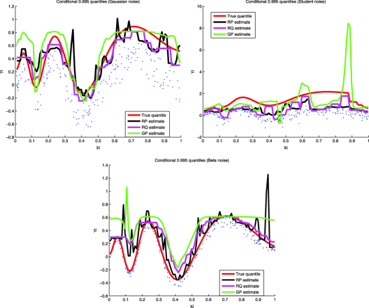
Figure 1: Typical realizations for simulated samples of size $n=200$. From left to right and from top to bottom, $Y|X$ is Gaussian, Student, Beta. The true quantile function $q(\beta_{n}|\cdot)$ in red with $\beta_{n}=1/n$. Its estimators $\hat{q}_{n}(\beta_{n}|\cdot)$ in magenta, $\tilde{q}^{\mathrm{RP},1}_{n}(\beta_{n}|\cdot)\equiv\tilde{q}^{\mathrm{RP},2}_{n}(\beta_{n}|\cdot)$ in black with $r=1/J$ and $J=3$, and $\hat{q}^{\mathrm{GP}}_{n}(\beta_{n}|\cdot)$ in green. The observations $(X_{i},Y_{i})$ are depicted as blue points.

4.3 Data-driven rules for selecting the parameters $h$ and $\alpha_{n}$

The use of the ‘RQ’ estimator $\hat{q}_{n}(\beta_{n}|x)\equiv\hat{q}_{n}(\beta_{n}|x;h)$, which relies on the inversion of $\hat{\bar{F}}_{n}(\cdot|\cdot)$, requires only the choice of the bandwidth $h$ in an interval $\mathcal{H}$ of lower and upper bounds given, respectively, by, say, $h_{\mathrm{min}}:=\max_{1\leq i<n}(X_{(i+1)}-X_{(i)})$ and $h_{\mathrm{max}}:=(X_{(n)}-X_{(1)})/4$. One way to select this parameter is by employing the cross-validation criterion as in [7] to obtain

$$h_{\mathrm{cv}}=\mathop{\arg\min}_{h\in\mathcal{H}}\sum_{i=1}^{n}\sum_{j=1}^{n}\bigl{\{}\mathbb{I}(Y_{i}\geq Y_{j})-\hat{\bar{F}}_{n,-i}(Y_{j}|X_{i})\bigr{\}}^{2},$$

where $\hat{\bar{F}}_{n,-i}(\cdot|\cdot)$ is the estimator $\hat{\bar{F}}_{n}(\cdot|\cdot)$ computed from the sample $\{(X_{j},Y_{j}),1\leq j\leq n,j\not=i\}$. The empirical procedure of [33] could be used to get the alternative data-driven global bandwidth

$$h_{yj}=h_{\mathrm{cv}}\biggl{(}\frac{\beta_{n}(1-\beta_{n})}{\phi(\Phi^{-1}(\beta_{n}))^{2}}\biggr{)}^{1/5},$$

where $\phi$ and $\Phi$ stand, respectively, for the standard normal density and distribution functions. However, the use of the ‘RP’ estimators $\tilde{q}^{\mathrm{RP},i}_{n}(\beta_{n}|x)$ and $\hat{\gamma}^{\mathrm{RP},i}_{n}(x)$, for $i=1,2$, requires in addition the selection of an appropriate order $\alpha_{n}$. To simplify the discussion, we set $\alpha_{n}$ at $k/n^{\star}_{xh}$, where the integer $k$ varies between $1$ and $n^{\star}_{xh}-1$, for each $h\in\mathcal{H}$. We also consider the value $J=3$ for which $\hat{\gamma}^{\mathrm{RP},1}_{n}(x)\equiv\hat{\gamma}^{\mathrm{RP},2}_{n}(x):=\hat{\gamma}^{\mathrm{RP}}_{n}(x;h,k)$ and $\tilde{q}^{\mathrm{RP},1}_{n}(\beta_{n}|x)\equiv\tilde{q}^{\mathrm{RP},2}_{n}(\beta_{n}|x):=\tilde{q}^{\mathrm{RP}}_{n}(\beta_{n}|x;h,k)$, with $r=1/J$. An empirical way to decide what values of $(h,k)$ should one use to compute the estimates in practice could be the automatic ad hoc data driven-rule employed in [6]. The main idea is to evaluate first the estimates, for each $x$ in a chosen grid of values, and then to select the parameters where the variation of the results is the smallest. This can be achieved in two ways:

Selecting $h$ and $k$ separately.

Step 1. Select a data-driven global bandwidth $h$, for example, $h_{\mathrm{cv}}$ or $h_{yj}$.

Step 2. Evaluate $\tilde{q}^{\mathrm{RP}}_{n}(\beta_{n}|x;h,k)$ at $k=1,\ldots,n^{\star}_{xh}-1$. Then compute the standard deviation of the estimates over a ‘window’ of (say $[\sqrt{n^{\star}_{xh}}]$) successive values of $k$. The value of $k$ where this standard deviation is minimal defines the desired parameter.

The same considerations evidently apply to $\hat{\gamma}^{\mathrm{RP}}_{n}(x)$ and to the ‘benchmark’ estimators $\hat{\gamma}^{\mathrm{GP}}_{n}(x):=\hat{\gamma}^{\mathrm{GP}}_{n}(x;h,k)$ and $\hat{q}^{\mathrm{GP}}_{n}(\beta_{n}|x):=\hat{q}^{\mathrm{GP}}_{n}(\beta_{n}|x;h,k)$, defined in Section 4.2, with the covariate dependent threshold being $u_{x}:=Y_{(n^{\star}_{xh}-k)}^{x}$, and $Y_{(1)}^{x}\leq\cdots\leq Y_{(n^{\star}_{xh})}^{x}$ being the sequence of ascending order statistics corresponding to the $Y_{i}$’s such that $|X_{i}-x|\leq h$.

The main difficulty when employing such a separate choice of $h$ and $k$ is that both $\tilde{q}^{\mathrm{RP}}_{n}(\beta_{n}|x;h_{\mathrm{cv}},k)$ and $\hat{q}^{\mathrm{GP}}_{n}(\beta_{n}|x;h_{\mathrm{cv}},k)$, respectively, $\hat{\gamma}^{\mathrm{RP}}_{n}(x;h_{\mathrm{cv}},k)$ and $\hat{\gamma}^{\mathrm{GP}}_{n}(x;h_{\mathrm{cv}},k)$, as functions of $k$ may be so unstable that reasonable values of $k$ (which would correspond to the true value of $q(\beta_{n}|x)$, respectively, $\gamma(x)$) may be hidden in the graphs. In result, the estimators may exhibit considerable volatility as functions of $x$ itself.

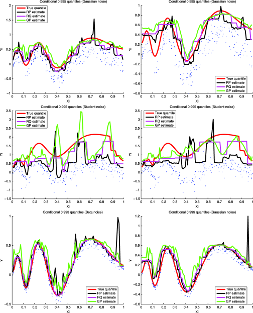
Figure 2: Separate parameters’ selection using the same simulated samples as in Figure 1. From left to right, the used bandwidth is $h_{\mathrm{cv}}$, $h_{yj}$. From top to bottom, $Y|X$ is Gaussian, Student, Beta. The true quantile function $q(\beta_{n}|\cdot)$ in red with $\beta_{n}=1/n$. Its estimators $\hat{q}_{n}(\beta_{n}|\cdot)$ in magenta, $\tilde{q}^{\mathrm{RP},1}_{n}(\beta_{n}|\cdot)\equiv\tilde{q}^{\mathrm{RP},2}_{n}(\beta_{n}|\cdot)$ in black with $r=1/J$ and $J=3$, and $\hat{q}^{\mathrm{GP}}_{n}(\beta_{n}|\cdot)$ in green. The observations $(X_{i},Y_{i})$ are depicted as blue points.

A typical realization is shown in Figure 2 when the bandwidths $h_{\mathrm{cv}}$ (left panels) and $h_{yj}$ (right panels) are used in Step 1. It may be seen that the method affords reasonable estimates in both Gaussian and Beta error models regarding the difficult curvature of the extreme quantile regression and the very small sample size $n=200$. However, it seems that the method fails in the case of Student noise, where the superiority of $\tilde{q}^{\mathrm{RP}}_{n}(\beta_{n}|\cdot)$ over both $\hat{q}^{\mathrm{GP}}_{n}(\beta_{n}|\cdot)$ and $\hat{q}_{n}(\beta_{n}|\cdot)$, demonstrated via the Monte Carlo study, is clearly sacrificed. This failure is probably due to the arbitrary choice $(3,1/3)$ of the parameters $(J,r)$ in $\tilde{q}^{\mathrm{RP}}_{n}(\beta_{n}|\cdot)$. It might also be seen that, apart from the student error model, the three estimators $\tilde{q}^{\mathrm{RP}}_{n}(\beta_{n}|\cdot)$, $\hat{q}_{n}(\beta_{n}|\cdot)$ and $\hat{q}^{\mathrm{GP}}_{n}(\beta_{n}|\cdot)$ point toward similar results.

Selecting $h$ and $k$ simultaneously.

Step 1. For each $h\in\mathcal{H}$, proceed to Step 2 described in the separate parameters’ selection. Set the value of $k$ where the standard deviation is minimal to be $k_{xh}$ and calculate the corresponding estimate $\tilde{q}^{\mathrm{RP}}_{n}(\beta_{n}|x;h,k_{xh})$.

Step 2. Compute the standard deviation of the estimates $\tilde{q}^{\mathrm{RP}}_{n}(\beta_{n}|x;h,k_{xh})$ over a window of (say $10$) successive values of $h$. Select the bandwidth where the standard deviation is minimal and then evaluate the corresponding estimate.

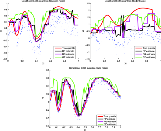
Figure 3: Simultaneous parameters’ selection using the same simulated samples as above. From left to right and from top to bottom, $Y|X$ is Gaussian, Student, Beta. The true quantile function $q(\beta_{n}|\cdot)$ in red with $\beta_{n}=1/n$. Its estimators $\hat{q}_{n}(\beta_{n}|\cdot)=\hat{q}_{n}(\beta_{n}|\cdot,h_{\mathrm{cv}})$ in magenta, $\tilde{q}^{\mathrm{RP},1}_{n}(\beta_{n}|\cdot)\equiv\tilde{q}^{\mathrm{RP},2}_{n}(\beta_{n}|\cdot)$ in black with $(r,J)=(1/3,3)$, and $\hat{q}^{\mathrm{GP}}_{n}(\beta_{n}|\cdot)$ in green. The $(X_{i},Y_{i})$’s are depicted as blue points.

In our simulations, we used a refined grid $\mathcal{H}$ of $50$ points between $\min(h_{\mathrm{cv}},h_{yj}-h_{\mathrm{cv}})$ and $h_{yj}+2h_{\mathrm{cv}}$. Any other limit bounds of $\mathcal{H}$ could of course be chosen near $h_{\mathrm{cv}}$ below and near $h_{yj}$ above. See Figure 3 for a typical realization in each simulated scenario. Here also the method is not without disadvantage as can be seen from the case of Student noise, where good results require a large sample size.

4.4 Concluding remarks

Monte Carlo evidence. The experiments indicate that $\hat{q}_{n}(\beta_{n}|x)$ is efficient relative to the modern smoothing estimator $\hat{q}^{\mathrm{GP}}_{n}(\beta_{n}|x)$ first introduced in [1, 2]. The simulations also indicate that the performance of the alternative estimator $\tilde{q}_{n}^{\mathrm{RP},1}(\beta_{n}|x)$ is quite remarkable in comparison with its analog $\tilde{q}_{n}^{\mathrm{RP},2}(\beta_{n}|x)$, at least in terms of MSE. In comparison with $\hat{q}_{n}(\beta_{n}|x)$ and $\hat{q}^{\mathrm{GP}}_{n}(\beta_{n}|x)$, the variability and the bias of both $\tilde{q}_{n}^{\mathrm{RP},1}(\beta_{n}|x)$ and $\tilde{q}_{n}^{\mathrm{RP},2}(\beta_{n}|x)$ are quite respectable and it seems that the heavier is the conditional tail, the better the estimators $\tilde{q}_{n}^{\mathrm{RP}}(\beta_{n}|x)$ are. It should be also clear that $\tilde{q}_{n}^{\mathrm{RP},1}(\beta_{n}|x)$ and $\tilde{q}_{n}^{\mathrm{RP},2}(\beta_{n}|x)$ can be improved appreciably by tuning the choice of the parameters $J$ and $r$.

Tuning parameters selection in practice. The simulations worked reasonably well for our ‘ad hoc’ selection methods except for the heavy-tailed case, corresponding to generally severe events. A sensible practice would be to verify whether the resulting ‘RP’, ‘GP’ and ‘RQ’ estimators point toward similar conclusions: the hard question of how to pick out the smoothing parameters $(h,k)$ simultaneously in an optimal way might thus become less urgent. In contrast, if the estimators look clearly different, this might diagnose a heavy-tailed conditional distribution with a great variability in severity: thereby our technique might be viewed as an exploratory tool, rather than as a method for final analysis. Doubtlessly, further work to define a concept of selecting appropriate values for the crucial parameters $(J,r)$ in the $\tilde{q}_{n}^{\mathrm{RP}}(\beta_{n}|x)$ estimators will yield new refinements.

The case of multiple covariates. We have discussed the asymptotic distributional properties of both estimators $\hat{q}_{n}(\beta_{n}|x)$ and $\tilde{q}_{n}^{\mathrm{RP}}(\beta_{n}|x)$ in detail in Sections 2 and 3 for multiple regressors $X\in\mathbb{R}^{p}$, but our contributions are probably only of a theoretical value in the case $p>1$. Indeed, as in the ordinary setting where the quantile order does not depend on the sample size, the kernel-smoothing method suffers from the ‘curse of dimensionality’. In our setting of extreme quantile regression, the curse is exacerbated by several degrees of magnitude and drastically increases in higher dimensions. To overcome this vexing defect, one can use dimension reduction techniques such as ADE (Average Derivative Estimator), see for instance [21]. Nevertheless, the theoretical properties of such methods are not yet established in the extreme-value framework.

5 Data example

Data on $123$ American electric utility companies were collected and the aim is to investigate the economic efficiency of these companies (see, e.g., [19]). A possible way to measure this efficiency is by looking at the maximum level of produced goods which is attainable for a given level of inputs-usage. From a statistical point of view, this problem translates into studying the upper boundary of the set of possible inputs $X$ and outputs $Y$, the so-called cost/econometric frontier in production theory. Hendricks and Koenker [22] stated: “In the econometric literature on the estimation of production technologies, there has been considerable interest in estimating so called frontier production models that correspond closely to models for extreme quantiles of a stochastic production surface”. The present paper may be viewed as the first ‘purely’ nonparametric work to actually investigate theoretically the idea of Hendricks and Koenker.

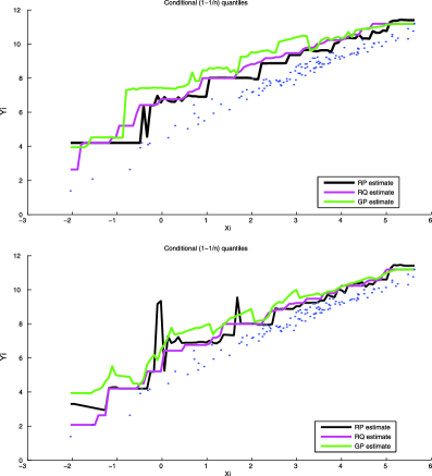
Figure 4: Scatterplot of the American electric utility data (blue points). Results obtained via the simultaneous (top) and separate (bottom) selection methods for $\beta_{n}=1/n$: the estimator $\hat{q}_{n}(\beta_{n}|\cdot)$ is drawn in magenta with $h_{yj}$ (top) and $h_{\mathrm{cv}}$ (bottom), $\hat{q}^{\mathrm{GP}}_{n}(\beta_{n}|\cdot)$ in green and $\tilde{q}^{\mathrm{RP},1}_{n}(\beta_{n}|\cdot)$ in black with $(r,J)=(1/3,3)$.

For our illustration purposes, we used the measurements on the variable $Y=\log(Q)$, with $Q$ being the production output of a firm, and the variable $X=\log(C)$, with $C$ being the total cost involved in the production. Figure 4 shows the $n=123$ observations, together with estimated extreme conditional quantiles $\hat{q}_{n}(\beta_{n}|x)$, $\hat{q}^{\mathrm{GP}}_{n}(\beta_{n}|x)$ and $\tilde{q}_{n}^{\mathrm{RP},1}(\beta_{n}|x)=\tilde{q}_{n}^{\mathrm{RP},2}(\beta_{n}|x)$ at $r=1/J$ with $J=3$. Given the small sample size, it was enough to use $\beta_{n}=1/n$ in describing the conditional distribution tails. For selecting the window width $h$ and the number $k$ of extremes, we maintained the automatic empirical data-driven rules described above. It appears that the extreme conditional quantile estimates are similar for both simultaneous (top) and separate (bottom) selection methods. Following their evolution, it may be seen that the American electric utility data do not correspond to the situation hoped for by the practitioners of a heavily short-tailed production process. Indeed, one may distinguish between two different behaviors of the extreme regression quantiles: They indicate a short-tailed conditional distribution for companies working at (transformed) input-factors larger than, say, $2$. In contrast, the tail distribution for the smallest companies with inputs $X_{i}<2$ seems to be moderately heavy. Therefore, the theoretical economic assumption that producers should operate on the upper boundary of the joint support of $(X,Y)$ rather than on its interior is clearly not fulfilled here, revealing a certain lack of production performance in this sector of activity. The estimated graph of $\tilde{q}_{n}^{\mathrm{RP},1}(\beta_{n}|x)$, $\hat{q}_{n}(\beta_{n}|x)$ or $\hat{q}^{\mathrm{GP}}_{n}(\beta_{n}|x)$ might be interpreted as the set of the most efficient firms. It is then clear that the firms achieve significantly lesser output than that predicted by the extremal quantile frontiers. This indicates a relative economic inefficiency especially in the population of the (sparse) smallest companies in terms of inputs.

Appendix: Proofs

.1 Preliminary results

We begin with a homogeneous property of the quantile function.

Lemma 1

Suppose (A.1) holds. If $\alpha_{n}\to 0$ as $n\to\infty$, then,

$$\lim_{n\to\infty}\frac{q(\xi\alpha_{n}|x)}{q(\alpha_{n}|x)}=\xi^{-(\gamma(x)\vee 0)}$$

for all $\xi>0$.

Proof.

From (4), we have

$$\frac{q(\xi\alpha_{n}|x)}{q(\alpha_{n}|x)}=1+K_{\gamma(x)}(1/\xi)\frac{a(q(\alpha_{n}|x)|x)}{q(\alpha_{n}|x)}\bigl{(}1+\mathrm{o}(1)\bigr{)}$$

and the conclusion follows using (5). ∎

The following lemma states that the convergence in (3) is uniform.

Lemma 2

Under (A.1), if $z_{n}(x)\uparrow y_{F}(x)$ as $n\to\infty$, then for all sequence of functions $t_{n}(x)$ such that $t_{n}(x)\to t_{0}(x)$ as $n\to\infty$ where $t_{0}(x)$ is such that there exists $\eta>0$ for which $1+\gamma(x)t_{0}(x)\geq\eta$ then,

$$\lim_{n\to\infty}\frac{\bar{F}(z_{n}(x)+t_{n}(x)a(z_{n}(x)|x)|x)}{\bar{F}(z_{n}(x)|x)}=\frac{1}{K_{\gamma(x)}^{-1}(t_{0}(x))}.$$

Proof.

Since $t_{n}(x)\to t_{0}(x)$ as $n\to\infty$, for all $\varepsilon_{1}>0$ such that $|\gamma(x)|\varepsilon_{1}<\eta$, there exists $N_{1}\geq 0$ such that for all $n\geq N_{1}$, $t_{0}(x)-\varepsilon_{1}\leq t_{n}(x)\leq t_{0}(x)+\varepsilon_{1}$. Since $a(z_{n}(x)|x)>0$ and $\bar{F}(\cdot|x)$ is a decreasing function, we have:

$$\frac{\bar{F}(z_{n}(x)+(t_{0}(x)+\varepsilon_{1})a(z_{n}(x)|x)|x)}{\bar{F}(z_{n}(x)|x)} \leq \frac{\bar{F}(z_{n}(x)+t_{n}(x)a(z_{n}(x)|x)|x)}{\bar{F}(z_{n}(x)|x)}$$

$$\leq \frac{\bar{F}(z_{n}(x)+(t_{0}(x)-\varepsilon_{1})a(z_{n}(x)|x)|x)}{\bar{F}(z_{n}(x)|x)}.$$

Now, since $|\gamma(x)|\varepsilon_{1}<\eta$, it is easy to check that $1+\gamma(x)(t_{0}(x)+\varepsilon_{1})\wedge 1+\gamma(x)(t_{0}(x)-\varepsilon_{1})>0$. Hence, under (A.1), for all $\varepsilon_{2}>0$, there exists $N_{2}\geq 0$ such that for all $n\geq N_{2}$

$$\frac{1-\varepsilon_{2}}{K_{\gamma(x)}^{-1}(t_{0}(x)+\varepsilon_{1})}\leq\frac{\bar{F}(z_{n}(x)+t_{n}(x)a(z_{n}(x)|x)|x)}{\bar{F}(z_{n}(x)|x)}\leq\frac{1+\varepsilon_{2}}{K_{\gamma(x)}^{-1}(t_{0}(x)-\varepsilon_{1})}.$$

Since $\varepsilon_{1}$ and $\varepsilon_{2}$ can be chosen arbitrarily small, this concludes the proof. ∎

Let us remark that the kernel estimator (1) can be rewritten as $\hat{\bar{F}}_{n}(y|x)=\hat{\psi}_{n}(y,x)/\hat{g}_{n}(x)$ where

$$\hat{\psi}_{n}(y,x)=\frac{1}{n}\sum_{i=1}^{n}K_{h}(x-X_{i})\mathbb{I}\{Y_{i}>y\}$$

is an estimator of $\psi(y,x)=\bar{F}(y|x)g(x)$ and $\hat{g}_{n}(x)$ is the classical kernel estimator of the p.d.f. $g(x)$ defined by:

$$\hat{g}_{n}(x)=\frac{1}{n}\sum_{i=1}^{n}K_{h}(x-X_{i}).$$

Lemma 3 gives standard results on the kernel estimator (see [26] for a proof) whereas Lemma 4 is dedicated to the asymptotic properties of $\hat{\psi}_{n}(y,x)$.

Lemma 3

Suppose (A.2), (A.3) hold. If $nh^{p}\to\infty$, then, for all $x\in\mathbb{R}^{p}$ such that $g(x)>0$, (

• ii)]

• $\mathbb{E}(\hat{g}_{n}(x)-g(x))=\mathrm{O}(h)$,

• $\operatorname{var}(\hat{g}_{n}(x))=\frac{g(x)\|K\|_{2}^{2}}{nh^{p}}(1+\mathrm{o}(1))$.

Therefore, under the assumptions of the above lemma, $\hat{g}_{n}(x)$ converges to $g(x)$ in probability.

Let us introduce some further notation. In the following, $y_{n}(x)$ is a sequence such that $y_{n}(x)\uparrow y_{F}(x)$ and $y_{n,j}(x)=y_{n}(x)+K_{\gamma(x)}(1/\tau_{j})a(y_{n}|x)(1+\mathrm{o}(1))$ for all $j=1,\ldots,K$. Recall that $0<\tau_{J}<\cdots<\tau_{2}<\tau_{1}\leq 1$. Moreover, the oscillations of the c.s.f. are controlled by

$$\omega_{n}(x):=\max_{j=1,\ldots,J}\sup_{x^{\prime}\in B(x,h)}\biggl{|}\frac{\bar{F}(y_{n,j}(x)|x^{\prime})}{\bar{F}(y_{n,j}(x)|x)}-1\biggr{|}.$$

Lemma 4

Suppose (A.1), (A.2) and (A.3) hold and let $x\in\mathbb{R}^{p}$ such that $g(x)>0$. If $\omega_{n}(x)\to 0$ and $nh^{p}\bar{F}(y_{n}(x)|x)\to\infty$ then, (

• ii)]

• $\mathbb{E}(\hat{\psi}_{n}(y_{n,j}(x),x))=\psi(y_{n,j}(x),x)(1+\mathrm{O}(\omega_{n}(x))+\mathrm{O}(h))$, for $j=1,\ldots,J$.

• The random vector

  $$\biggl{\{}\sqrt{nh^{p}\psi\bigl{(}y_{n}(x),x\bigr{)}}\biggl{(}\frac{\hat{\psi}_{n}(y_{n,j}(x),x)-\mathbb{E}(\hat{\psi}_{n}(y_{n,j}(x),x))}{\psi(y_{n,j}(x),x)}\biggr{)}\biggr{\}}_{j=1,\ldots,J}$$

  is asymptotically Gaussian, centered, with covariance matrix $\|K\|_{2}^{2}V$ where $V_{j,j^{\prime}}=\tau^{-1}_{j\wedge j^{\prime}}$ for $(j,j^{\prime})\in\{1,\ldots,J\}^{2}$.

Proof.

(i) Since the $(X_{i},Y_{i})$, $i=1,\ldots,n$ are identically distributed, we have

$$\mathbb{E}\bigl{(}\hat{\psi}_{n}\bigl{(}y_{n,j}(x),x\bigr{)}\bigr{)} = \int_{\mathbb{R}^{p}}K_{h}(x-t)\bar{F}\bigl{(}y_{n,j}(x)|t\bigr{)}g(t)\,\mathrm{d}t$$

$$= \int_{S}K(u)\bar{F}\bigl{(}y_{n,j}(x)|x-hu\bigr{)}g(x-hu)\,\mathrm{d}u,$$

under (A.3). Let us now consider

$$\bigl{|}\mathbb{E}\bigl{(}\hat{\psi}_{n}\bigl{(}y_{n,j}(x),x\bigr{)}\bigr{)}-\psi\bigl{(}y_{n,j}(x),x\bigr{)}\bigr{|}$$

(8)

$$\quad\leq\bar{F}\bigl{(}y_{n,j}(x)|x\bigr{)}\int_{S}K(u)\bigl{|}g(x-hu)-g(x)\bigr{|}\,\mathrm{d}u$$

$$\qquad{}+\bar{F}\bigl{(}y_{n,j}(x)|x\bigr{)}\int_{S}K(u)\biggl{|}\frac{\bar{F}(y_{n,j}(x)|x-hu)}{\bar{F}(y_{n,j}(x)|x)}-1\biggr{|}g(x-hu)\,\mathrm{d}u.$$ (9)

Under (A.2), and since $g(x)>0$, we have

$$(\ref{eq1})\leq\bar{F}\bigl{(}y_{n,j}(x)|x\bigr{)}c_{g}h\int_{S}\,\mathrm{d}(u,0)K(u)\,\mathrm{d}u=\psi\bigl{(}y_{n,j}(x),x\bigr{)}\mathrm{O}(h),$$ (10)

and, in view of (10),

$$(\ref{eq2}) \leq \bar{F}\bigl{(}y_{n,j}(x)|x\bigr{)}\omega_{n}(x)\int_{S}K(u)g(x-hu)\,\mathrm{d}u=\bar{F}\bigl{(}y_{n,j}(x)|x\bigr{)}\omega_{n}(x)g(x)\bigl{(}1+\mathrm{o}(1)\bigr{)}$$

$$= \psi\bigl{(}y_{n,j}(x),x\bigr{)}\omega_{n}(x)\bigl{(}1+\mathrm{o}(1)\bigr{)}.$$

Combining (10) and (.1) concludes the first part of the proof.

(ii) Let $\beta\neq 0$ in $\mathbb{R}^{J}$, $\Lambda_{n}(x)=(nh^{p}\psi(y_{n}(x),x))^{-1/2}$, and consider the random variable

$$\Psi_{n} = \sum_{j=1}^{J}\beta_{j}\biggl{(}\frac{\hat{\psi}_{n}(y_{n,j}(x),x)-\mathbb{E}(\hat{\psi}_{n}(y_{n,j}(x),x))}{\Lambda_{n}(x)\psi(y_{n,j}(x),x)}\biggr{)}$$

$$= \sum_{i=1}^{n}\frac{1}{n\Lambda_{n}(x)}\Biggl{\{}\sum_{j=1}^{J}\frac{\beta_{j}K_{h}(x-X_{i})\mathbb{I}\{Y_{i}\geq y_{n,j}(x)\}}{\psi(y_{n,j}(x),x)}$$

$$\hskip 46.0pt\quad{}-\mathbb{E}\Biggl{(}\sum_{j=1}^{J}\frac{\beta_{j}K_{h}(x-X_{i})\mathbb{I}\{Y_{i}\geq y_{n,j}(x)\}}{\psi(y_{n,j}(x),x)}\Biggr{)}\Biggr{\}}$$

$$:= \sum_{i=1}^{n}Z_{i,n}.$$

Clearly, $\{Z_{i,n},i=1,\ldots,n\}$ is a set of centered, independent and identically distributed random variables with variance

$$\operatorname{var}(Z_{i,n})=\frac{1}{n^{2}h^{2p}\Lambda_{n}^{2}(x)}\operatorname{var}\Biggl{(}\sum_{j=1}^{J}\beta_{j}K\biggl{(}\frac{x-X_{i}}{h}\biggr{)}\frac{\mathbb{I}\{Y_{i}\geq y_{n,j}(x)\}}{\psi(y_{n,j}(x),x)}\Biggr{)}=\frac{1}{n^{2}h^{p}\Lambda_{n}^{2}(x)}\beta^{t}B\beta,$$

where $B$ is the $J\times J$ covariance matrix with coefficients defined for $(j,j^{\prime})\in\{1,\ldots,J\}^{2}$ by

$$B_{j,j^{\prime}} = \frac{A_{j,j^{\prime}}}{\psi(y_{n,j}(x),x)\psi(y_{n,j^{\prime}}(x),x)},$$

$$A_{j,j^{\prime}} = \frac{1}{h^{p}}\operatorname{cov}\biggl{(}K\biggl{(}\frac{x-X}{h}\biggr{)}\mathbb{I}\bigl{\{}Y\geq y_{n,j}(x)\bigr{\}},K\biggl{(}\frac{x-X}{h}\biggr{)}\mathbb{I}\bigl{\{}Y\geq y_{n,j^{\prime}}(x)\bigr{\}}\biggr{)}$$

$$= \|K\|_{2}^{2}\mathbb{E}\biggl{(}\frac{1}{h^{p}}Q\biggl{(}\frac{x-X}{h}\biggr{)}\mathbb{I}\bigl{\{}Y\geq y_{n,j}(x)\vee y_{n,j^{\prime}}(x)\bigr{\}}\biggr{)}$$

$${}-h^{p}\mathbb{E}\bigl{(}K_{h}(x-X)\mathbb{I}\bigl{\{}Y\geq y_{n,j}(x)\bigr{\}}\bigr{)}\mathbb{E}\bigl{(}K_{h}(x-X)\mathbb{I}\bigl{\{}Y\geq y_{n,j^{\prime}}(x)\bigr{\}}\bigr{)},$$

with $Q(\cdot):=K^{2}(\cdot)/\|K\|^{2}_{2}$ also satisfying assumption (A.3). As a consequence, the three above expectations are of the same nature. Thus, remarking that, for $n$ large enough, $y_{n,j}(x)\vee y_{n,j^{\prime}}(x)=y_{n,j\vee j^{\prime}}(x)$, part (i) of the proof implies

$$A_{j,j^{\prime}} = \|K\|^{2}_{2}\psi\bigl{(}y_{n,j\vee j^{\prime}}(x),x\bigr{)}\bigl{(}1+\mathrm{O}\bigl{(}\omega_{n}(x)\bigr{)}+\mathrm{O}(h)\bigr{)}$$

$${}-h^{p}\psi\bigl{(}y_{n,j}(x),x\bigr{)}\psi\bigl{(}y_{n,j^{\prime}}(x),x\bigr{)}\bigl{(}1+\mathrm{O}\bigl{(}\omega_{n}(x)\bigr{)}+\mathrm{O}(h)\bigr{)}$$

leading to

$$B_{j,j^{\prime}} = \frac{\|K\|^{2}_{2}}{\psi(y_{n,j\wedge j^{\prime}}(x),x)}\bigl{(}1+\mathrm{O}\bigl{(}\omega_{n}(x)\bigr{)}+\mathrm{O}(h)\bigr{)}-h^{p}\bigl{(}1+\mathrm{O}\bigl{(}\omega_{n}(x)\bigr{)}+\mathrm{O}(h)\bigr{)}$$

$$= \frac{\|K\|^{2}_{2}}{\psi(y_{n,j\wedge j^{\prime}}(x),x)}\bigl{(}1+\mathrm{o}(1)\bigr{)},$$

since $\psi(y_{n,j\wedge j^{\prime}}(x),x)\to 0$ as $n\to\infty$. Now, from Lemma 2,

$$\lim_{n\to\infty}\frac{\psi(y_{n,j\wedge j^{\prime}}(x),x)}{\psi(y_{n}(x),x)}=\frac{1}{K_{\gamma(x)}^{-1}(K_{\gamma(x)}(1/\tau_{j\wedge j^{\prime}}))}=\tau_{j\wedge j^{\prime}}$$

entailing

$$B_{j,j^{\prime}}=\frac{\|K\|^{2}_{2}V_{j,j^{\prime}}}{\psi(y_{n}(x),x)}\bigl{(}1+\mathrm{o}(1)\bigr{)},$$

and therefore, $\operatorname{var}(Z_{i,n})\sim\|K\|^{2}_{2}\beta^{t}V\beta/n,$ for all $i=1,\ldots,n$. As a preliminary conclusion, the variance of $\Psi_{n}$ converges to $\|K\|^{2}_{2}\beta^{t}V\beta$. Consequently, Lyapounov criteria for the asymptotic normality of sums of triangular arrays reduces to $\sum_{i=1}^{n}\mathbb{E}|Z_{i,n}|^{3}=n\mathbb{E}|Z_{1,n}|^{3}\rightarrow 0.$ Remark that $Z_{1,n}$ is a bounded random variable:

$$|Z_{1,n}| \leq \frac{2\|K\|_{\infty}\sum_{j=1}^{J}|\beta_{j}|}{n\Lambda_{n}(x)h^{p}\psi(y_{n,J},x)}$$

$$= \frac{2}{\tau_{J}}\|K\|_{\infty}\sum_{j=1}^{J}|\beta_{j}|\Lambda_{n}(x)\bigl{(}1+\mathrm{o}(1)\bigr{)}$$

and thus,

$$n\mathbb{E}|Z_{1,n}|^{3} \leq \frac{2}{\tau_{J}}\|K\|_{\infty}\sum_{j=1}^{J}n|\beta_{j}|\Lambda_{n}(x){\operatorname{var}}(Z_{1,n})\bigl{(}1+\mathrm{o}(1)\bigr{)}$$

$$= \frac{2}{\tau_{J}}\|K\|_{\infty}\|K\|^{2}_{2}\sum_{j=1}^{J}|\beta_{j}|\beta^{t}V\beta\Lambda_{n}(x)\bigl{(}1+\mathrm{o}(1)\bigr{)}\to 0$$

as $n\to\infty$. As a conclusion, $\Psi_{n}$ converges in distribution to a centered Gaussian random variable with variance $\|K\|^{2}_{2}\beta^{t}V\beta$ for all $\beta\neq 0$ in $\mathbb{R}^{p}$. The result is proved. ∎

Let us now focus on the estimation of small tail probabilities $\bar{F}(y_{n}(x)|x)$ when $y_{n}(x)\uparrow y_{F}(x)$ as $n\to\infty$. The following result provides sufficient conditions for the asymptotic normality of $\hat{\bar{F}}_{n}(y_{n}(x)|x)$.

Proposition 0

Suppose (A.1), (A.2) and (A.3) hold and let $x\in\mathbb{R}^{p}$ such that $g(x)>0$. If $nh^{p}\bar{F}(y_{n}(x)|x)\to\infty$ and $nh^{p}\bar{F}(y_{n}(x)|x)(h\vee\omega_{n}(x))^{2}\to 0$, then, the random vector

$$\biggl{\{}\sqrt{nh^{p}\bar{F}\bigl{(}y_{n}(x)|x\bigr{)}}\biggl{(}\frac{\hat{\bar{F}}_{n}(y_{n,j}(x)|x)}{\bar{F}(y_{n,j}(x)|x)}-1\biggr{)}\biggr{\}}_{j=1,\ldots,J}$$

is asymptotically Gaussian, centered, with covariance matrix $\|K\|_{2}^{2}/g(x)V$ where $V_{j,j^{\prime}}=\tau^{-1}_{j\wedge j^{\prime}}$ for $(j,j^{\prime})\in\{1,\ldots,J\}^{2}$.

Proof.

Keeping in mind the notation of Lemma 4, the following expansion holds

$$\Lambda_{n}^{-1}(x)\sum_{j=1}^{J}\beta_{j}\biggl{(}\frac{\hat{\bar{F}}_{n}(y_{n,j}(x)|x)}{\bar{F}(y_{n,j}(x)|x)}-1\biggr{)}=\frac{T_{1,n}+T_{2,n}-T_{3,n}}{\hat{g}_{n}(x)},$$ (12)

where

$$T_{1,n} = g(x)\Lambda_{n}^{-1}(x)\sum_{j=1}^{J}\beta_{j}\biggl{(}\frac{\hat{\psi}_{n}(y_{n,j}(x),x)-\mathbb{E}(\hat{\psi}_{n}(y_{n,j}(x),x))}{\psi(y_{n,j}(x),x)}\biggr{)},$$

$$T_{2,n} = g(x)\Lambda_{n}^{-1}(x)\sum_{j=1}^{J}\beta_{j}\biggl{(}\frac{\mathbb{E}(\hat{\psi}_{n}(y_{n,j}(x),x))-\psi(y_{n,j}(x),x)}{\psi(y_{n,j}(x),x)}\biggr{)},$$

$$T_{3,n} = \Biggl{(}\sum_{j=1}^{J}\beta_{j}\Biggr{)}\Lambda_{n}^{-1}(x)\bigl{(}\hat{g}_{n}(x)-g(x)\bigr{)}.$$

Let us highlight that assumptions $nh^{p}\bar{F}(y_{n}(x)|x)\omega_{n}^{2}(x)\to 0$ and $nh^{p}\bar{F}(y_{n}(x)|x)\to\infty$ imply that $\omega_{n}(x)\to 0$ as $n\to\infty$. Thus, from Lemma 4(ii), the random term $T_{1,n}$ can be rewritten as

$$T_{1,n}=g(x)\|K\|_{2}\sqrt{\beta^{t}V\beta}\xi_{n},$$ (13)

where $\xi_{n}$ converges to a standard Gaussian random variable. The nonrandom term $T_{2,n}$ is controlled with Lemma 4(i):

$$T_{2,n}=\mathrm{O}(\Lambda_{n}^{-1}(x)\bigl{(}h+\Delta\bigl{(}y_{n}(x),x\bigr{)}\bigr{)}=\mathrm{O}\bigl{(}\bigl{(}nh^{p}\bar{F}\bigl{(}y_{n}(x)|x\bigr{)}\bigr{)}^{1/2}\bigl{(}h\vee\omega_{n}(x)\bigr{)}\bigr{)}=\mathrm{o}(1).$$ (14)

Finally, $T_{3,n}$ is a classical term in kernel density estimation, which can be bounded by Lemma 3:

$$T_{3,n} = \mathrm{O}\bigl{(}h\Lambda_{n}^{-1}(x)\bigr{)}+\mathrm{O}_{P}\bigl{(}\Lambda_{n}^{-1}(x)\bigl{(}nh^{p}\bigr{)}^{-1/2}\bigr{)}$$

$$= \mathrm{O}\bigl{(}nh^{p+2}\bar{F}\bigl{(}y_{n}(x)|x\bigr{)}\bigr{)}^{1/2}+\mathrm{O}_{P}\bigl{(}\bar{F}\bigl{(}y_{n}(x)|x\bigr{)}\bigr{)}^{1/2}=\mathrm{o}_{P}(1).$$

Collecting (12)–(.1), it follows that

$$\hat{g}_{n}(x)\Lambda_{n}^{-1}(x)\sum_{j=1}^{J}\beta_{j}\biggl{(}\frac{\hat{\bar{F}}_{n}(y_{n,j}(x)|x)}{\bar{F}(y_{n,j}(x)|x)}-1\biggr{)}=g(x)\|K\|_{2}\sqrt{\beta^{t}V\beta}\xi_{n}+\mathrm{o}_{P}(1).$$

Finally, $\hat{g}_{n}(x)\stackrel{{\scriptstyle P}}{{\longrightarrow}}g(x)$ yields

$$\sqrt{nh^{p}\bar{F}\bigl{(}y_{n}(x)|x\bigr{)}}\sum_{j=1}^{J}\beta_{j}\biggl{(}\frac{\hat{\bar{F}}_{n}(y_{n,j}(x)|x)}{\bar{F}(y_{n,j}(x)|x)}-1\biggr{)}$$

$$\quad=\|K\|_{2}\sqrt{\frac{\beta^{t}V\beta}{g(x)}}\xi_{n}+\mathrm{o}_{P}(1)$$

and the result is proved. ∎

The last lemma establishes that $K_{\hat{\gamma}_{n}(x)}(r_{n})$ inherits from the convergence properties of $\hat{\gamma}_{n}(x)$.

Lemma 5

Suppose $\xi_{n}^{(\gamma)}(x):=\Lambda_{n}^{-1}(\hat{\gamma}_{n}(x)-\gamma(x))=\mathrm{O}_{\mathbb{P}}(1)$, where $\Lambda_{n}\to 0$. Let $r_{n}\geq 1$ or $r_{n}\leq 1$ such that $\Lambda_{n}\log(r_{n})\to 0$. Then,

$$\Lambda_{n}^{-1}\biggl{(}\frac{K_{\hat{\gamma}_{n}(x)}(r_{n})-K_{\gamma(x)}(r_{n})}{K^{\prime}_{\gamma(x)}(r_{n})}\biggr{)}=\xi_{n}^{(\gamma)}(x)\bigl{(}1+\mathrm{o}_{\mathbb{P}}(1)\bigr{)}.$$

Proof.

Since $\hat{\gamma}_{n}(x)\stackrel{{\scriptstyle P}}{{\longrightarrow}}\gamma(x)$, a first order Taylor expansion yields

$$K_{\hat{\gamma}_{n}(x)}(r_{n})=K_{\gamma(x)}(r_{n})+\Lambda_{n}\xi_{n}^{(\gamma)}(x)K^{\prime}_{\tilde{\gamma}_{n}(x)}(r_{n}),$$

where $\tilde{\gamma}_{n}(x)=\gamma(x)+\Theta_{n}\Lambda_{n}\xi_{n}^{(\gamma)}(x)$ with $\Theta_{n}\in(0,1)$. As a consequence

$$\Lambda_{n}^{-1}\biggl{(}\frac{K_{\hat{\gamma}_{n}(x)}(r_{n})-K_{\gamma(x)}(r_{n})}{K^{\prime}_{\gamma(x)}(r_{n})}\biggr{)} = \xi_{n}^{(\gamma)}(x)\frac{K^{\prime}_{\tilde{\gamma}_{n}(x)}(r_{n})}{K^{\prime}_{\gamma(x)}(r_{n})}$$

$$= \xi_{n}^{(\gamma)}(x)\biggl{(}1+\frac{\int_{1}^{r_{n}}(s^{\tilde{\gamma}_{n}(x)-\gamma(x)}-1)s^{\gamma(x)-1}\log(s)\,\mathrm{d}s}{\int_{1}^{r_{n}}s^{\gamma(x)-1}\log(s)\,\mathrm{d}s}\biggr{)}.$$

Suppose for instance $r_{n}\geq 1$. The assumptions yield $(\log r_{n})(\tilde{\gamma}_{n}(x)-\gamma(x))\stackrel{{\scriptstyle P}}{{\longrightarrow}}0$ and thus, for $n$ large enough, with high probability,

$$\sup_{s\in[1,r_{n}]}\bigl{|}\bigl{(}s^{\tilde{\gamma}_{n}(x)-\gamma(x)}-1\bigr{)}\bigr{|}\leq 2(\log r_{n})\bigl{|}\tilde{\gamma}_{n}(x)-\gamma(x)\bigr{|}=\mathrm{o}_{\mathbb{P}}(1).$$

As a conclusion,

$$\Lambda_{n}^{-1}\biggl{(}\frac{K_{\hat{\gamma}_{n}(x)}(r_{n})-K_{\gamma(x)}(r_{n})}{K^{\prime}_{\gamma(x)}(r_{n})}\biggr{)}=\xi^{(\gamma)}(x)\bigl{(}1+\mathrm{o}_{\mathbb{P}}(1)\bigr{)}$$

and the result is proved. The case $r_{n}\leq 1$ is easily deduced since $K_{\gamma(x)}(1/r_{n})=-K_{-\gamma(x)}(r_{n})$ and $K^{\prime}_{\gamma(x)}(1/r_{n})=K^{\prime}_{-\gamma(x)}(r_{n})$. ∎

.2 Proofs of main results

Proof of Theorem 1 Let us introduce $v_{n}=(nh^{p}\alpha_{n}^{-1})^{1/2}$, $\sigma_{n}(x)=(v_{n}f(q(\alpha_{n}|x)|x))^{-1}$ and, for all $j=1,\ldots,J$,

$$W_{n,j}(x) = v_{n}\bigl{(}\hat{\bar{F}}_{n}\bigl{(}q(\tau_{j}\alpha_{n}|x)+\sigma_{n}(x)z_{j}|x\bigr{)}-\bar{F}\bigl{(}q(\tau_{j}\alpha_{n}|x)+\sigma_{n}(x)z_{j}|x\bigr{)}\bigr{)},$$

$$a_{n,j}(x) = v_{n}\bigl{(}\tau_{j}\alpha_{n}-\bar{F}\bigl{(}q(\alpha_{n,j}|x)+\sigma_{n}(x)z_{j}|x\bigr{)}\bigr{)}$$

and $z_{j}\in\mathbb{R}$. We examine the asymptotic behavior of $J$-variate function defined by

$$\Phi_{n}(z_{1},\ldots,z_{J}) = \mathbb{P}\Biggl{(}\bigcap_{j=1}^{J}\bigl{\{}\sigma_{n}^{-1}(x)\bigl{(}\hat{q}_{n}(\tau_{j}\alpha_{n}|x)-q(\tau_{j}\alpha_{n}|x)\bigr{)}\leq z_{j}\bigr{\}}\Biggr{)}$$

$$= \mathbb{P}\Biggl{(}\bigcap_{j=1}^{J}\bigl{\{}W_{n,j}(x)\leq a_{n,j}(x)\bigr{\}}\Biggr{)}.$$

Let us first focus on the nonrandom term $a_{n,j}(x)$. For each $j\in\{1,\ldots,J\}$ there exists $\theta_{n,j}\in(0,1)$ such that

$$a_{n,j}(x)=v_{n}\sigma_{n}(x)z_{j}f\bigl{(}q_{n,j}(x)|x\bigr{)}=z_{j}\frac{f(q_{n,j}(x)|x)}{f(q(\alpha_{n}|x)|x)},$$

where

$$q_{n,j}(x) = q(\tau_{j}\alpha_{n}|x)+\theta_{n,j}\sigma_{n}(x)z_{j}$$

$$= q(\tau_{j}\alpha_{n}|x)+\theta_{n,j}\frac{z_{j}}{\tau_{j}}\bigl{(}nh^{p}\alpha_{n}\bigr{)}^{-1/2}\frac{\tau_{j}\alpha_{n}}{f(q(\tau_{j}\alpha_{n}|x)|x)}\frac{f(q(\tau_{j}\alpha_{n}|x)|x)}{f(q(\alpha_{n}|x)|x)}$$

$$= q(\tau_{j}\alpha_{n}|x)+\theta_{n,j}z_{j}\tau_{j}^{\gamma(x)}\bigl{(}nh^{p}\alpha_{n}\bigr{)}^{-1/2}\frac{\tau_{j}\alpha_{n}}{f(q(\tau_{j}\alpha_{n}|x)|x)}\bigl{(}1+\mathrm{o}(1)\bigr{)},$$

since $y\mapsto f(q(y|x)|x)$ is regularly varying at 0 with index $\gamma(x)+1$, see [10], Corollary 1.1.10, equation (1.1.33). Now, in view of [10], Theorem 1.2.6 and [10], Remark 1.2.7, a possible choice of the auxiliary function is

$$a(t|x)=\frac{\bar{F}(t|x)}{f(t|x)}\bigl{(}1+\mathrm{o}(1)\bigr{)},$$ (16)

leading to

$$q_{n,j}(x)=q(\tau_{j}\alpha_{n}|x)+\theta_{n,j}z_{j}\tau_{j}^{\gamma(x)}\bigl{(}nh^{p}\alpha_{n}\bigr{)}^{-1/2}a\bigl{(}q(\tau_{j}\alpha_{n}|x)|x\bigr{)}\bigl{(}1+\mathrm{o}(1)\bigr{)}.$$

Applying Lemma 2 with $z_{n}(x)=q(\tau_{j}\alpha_{n}|x)$, $t_{n}(x)=\theta_{n,j}z_{j}\tau_{j}^{\gamma(x)}(nh^{p}\alpha_{n})^{-1/2}(1+\mathrm{o}(1))$ and $t_{0}(x)=0$ yields

$$\frac{\bar{F}(q_{n,j}(x)|x)}{\tau_{j}\alpha_{n}}\to K_{\gamma(x)}^{-1}(0)=1$$

as $n\to\infty$. Recalling that $y\mapsto f(q(y|x)|x)$ is regularly varying, we have

$$\frac{f(q_{n,j}(x)|x)}{f(q(\alpha_{n}|x)|x)}\to\tau_{j}^{\gamma(x)+1}$$

as $n\to\infty$ and therefore

$$a_{n,j}(x)=z_{j}\tau_{j}^{\gamma(x)+1}\bigl{(}1+\mathrm{o}(1)\bigr{)},\qquad j=1,\ldots,J.$$ (17)

Let us now turn to the random term $W_{n,j}(x)$. Let us define $z_{n,j}(x)=q(\tau_{j}\alpha_{n}|x)+\sigma_{n}(x)z_{j}$ for $j=1,\ldots,J$, $y_{n}(x)=q(\alpha_{n}|x)$, and consider the expansion

$$\frac{z_{n,j}(x)-y_{n}(x)}{a(y_{n}(x)|x)}=\frac{q(\tau_{j}\alpha_{n}|x)-q(\alpha_{n}|x)}{a(q(\alpha_{n}|x)|x)}+\frac{\sigma_{n}(x)z_{j}}{a(q(\alpha_{n}|x)|x)}.$$

From (4), we have

$$\lim_{n\to\infty}\frac{q(\tau_{j}\alpha_{n}|x)-q(\alpha_{n}|x)}{a(q(\alpha_{n}|x)|x)}=K_{\gamma(x)}(1/\tau_{j}),$$

and

$$\lim_{n\to\infty}\frac{\sigma_{n}(x)z_{j}}{a(q(\alpha_{n}|x)|x)}=0,$$

leading to $z_{n,j}(x)=y_{n}(x)+K_{\gamma(x)}(1/\tau_{j})a(y_{n}(x)|x)(1+\mathrm{o}(1))$. Introducing $\beta_{n,j}(x)=\bar{F}(y_{n,j}(x)|x)$, the oscillation $\omega_{n}(x)$ can be rewritten as

$$\omega_{n}(x)=\max_{j=1,\ldots,J}\sup_{x^{\prime}\in B(x,h)}\biggl{|}\frac{\bar{F}(q(\beta_{n,j}(x)|x)|x^{\prime})}{\beta_{n,j}(x)}-1\biggr{|}.$$

For all $\kappa\in(0,\tau_{J})$ and $j=1,\ldots,J$, we eventually have $z_{n,j}(x)\in[y_{n}(x),z_{n}(x)]$ where $z_{n}(x):=y_{n}(x)+K_{\gamma(x)}(2/\kappa)a(y_{n}(x)|x)$ and thus $\beta_{n,j}(x)\in[\bar{F}(z_{n}(x)|x),\alpha_{n}]$ eventually. Now, Lemma 2 implies that $\bar{F}(z_{n}(x)|x)/\alpha_{n}\to\kappa/2$ as $n\to\infty$ and thus, for $n$ large enough, $\beta_{n,j}(x)\in[\kappa\alpha_{n},\alpha_{n}]$. Consequently, $\omega_{n}(x)\leq\Delta_{\kappa}(\alpha_{n},x)$. Applying Proposition 1 and Lemma 2 yields

$$W_{n,j}(x)=\frac{\bar{F}(z_{n,j}(x)|x)}{\alpha_{n}}\xi_{n,j}={\tau_{j}}\xi_{n,j}\bigl{(}1+\mathrm{o}(1)\bigr{)},$$

where $\xi_{n}=(\xi_{n,1},\ldots,\xi_{n,j})^{t}$ converges to a centered Gaussian random vector with covariance matrix $\|K\|_{2}^{2}/g(x)V$. Taking into account of (17), the results follows.

Proof of Corollary 1 Let us remark that, from (16),

$$\Bigl{\{}f\bigl{(}q(\alpha_{n}|x)|x\bigr{)}\sqrt{nh^{p}\alpha_{n}^{-1}}\bigl{(}\hat{q}_{n}(\tau_{j}\alpha_{n}|x)-q(\tau_{j}\alpha_{n}|x)\bigr{)}\Bigr{\}}_{j=1,\ldots,J}$$

$$\quad=\biggl{\{}q(\alpha_{n}|x)\frac{f(q(\alpha_{n}|x)|x)}{\alpha_{n}}\frac{q(\tau_{j}\alpha_{n}|x)}{q(\alpha_{n}|x)}\sqrt{nh^{p}\alpha_{n}}\biggl{(}\frac{\hat{q}_{n}(\tau_{j}\alpha_{n}|x)}{q(\tau_{j}\alpha_{n}|x)}-1\biggr{)}\biggr{\}}_{j=1,\ldots,J}$$

$$\quad=\biggl{\{}\frac{q(\alpha_{n}|x)}{a(q(\alpha_{n}|x)|x)}\frac{q(\tau_{j}\alpha_{n}|x)}{q(\alpha_{n}|x)}\sqrt{nh^{p}\alpha_{n}}\biggl{(}\frac{\hat{q}_{n}(\tau_{j}\alpha_{n}|x)}{q(\tau_{j}\alpha_{n}|x)}-1\biggr{)}\biggr{\}}_{j=1,\ldots,J}\bigl{(}1+\mathrm{o}(1)\bigr{)}$$

$$\quad=\biggl{\{}\frac{q(\alpha_{n}|x)}{a(q(\alpha_{n}|x)|x)}\tau_{j}^{-(\gamma(x)\vee 0)}\sqrt{nh^{p}\alpha_{n}}\biggl{(}\frac{\hat{q}_{n}(\tau_{j}\alpha_{n}|x)}{q(\tau_{j}\alpha_{n}|x)}-1\biggr{)}\biggr{\}}_{j=1,\ldots,J}\bigl{(}1+\mathrm{o}(1)\bigr{)},$$

in view of Lemma 1. The result follows from Theorem 1.

Proof of Theorem 2 By definition,

$$q_{n}(\beta_{n}|x)=q_{n}(\alpha_{n}|x)+\bigl{(}K_{\gamma(x)}(\alpha_{n}/\beta_{n})+b(\beta_{n}/\alpha_{n},\alpha_{n})\bigr{)}a\bigl{(}q(\alpha_{n}|x)|x\bigr{)}$$

and thus, the following expansion can be easily established:

$$\Lambda_{n}^{-1}\biggl{(}\frac{\tilde{q}_{n}(\beta_{n}|x)-q(\beta_{n}|x)}{a(q(\alpha_{n}|x)|x)K^{\prime}_{\gamma(x)}(\alpha_{n}/\beta_{n})}\biggr{)}$$

$$\quad=\Lambda_{n}^{-1}\biggl{(}\frac{\hat{q}_{n}(\alpha_{n}|x)-q(\alpha_{n}|x)}{a(q(\alpha_{n}|x)|x)K^{\prime}_{\gamma(x)}(\alpha_{n}/\beta_{n})}\biggr{)}$$

$$\qquad{}+\Lambda_{n}^{-1}\biggl{(}\frac{K_{\hat{\gamma}_{n}(x)}(\alpha_{n}/\beta_{n})-K_{\gamma(x)}(\alpha_{n}/\beta_{n})}{K^{\prime}_{\gamma(x)}(\alpha_{n}/\beta_{n})}\biggr{)}\frac{\hat{a}_{n}(x)}{a(q(\alpha_{n}|x)|x)}$$

$$\qquad{}+\Lambda_{n}^{-1}\frac{K_{\gamma(x)}(\alpha_{n}/\beta_{n})}{K^{\prime}_{\gamma(x)}(\alpha_{n}/\beta_{n})}\biggl{(}\frac{\hat{a}_{n}(x)}{a(q(\alpha_{n}|x)|x)}-1\biggr{)}$$

$$\qquad{}+\Lambda_{n}^{-1}\frac{b(\beta_{n}/\alpha_{n},\alpha_{n})}{K^{\prime}_{\gamma(x)}(\alpha_{n}/\beta_{n})}$$

$$\quad=:T_{n,1}+T_{n,2}+T_{n,3}+T_{n,4}.$$

Introducing

$$\bigl{(}\xi_{n}^{(\gamma)}(x),\xi_{n}^{(a)}(x),\xi_{n}^{(q)}(x)\bigr{)}:=\Lambda_{n}^{-1}\biggl{(}\hat{\gamma}_{n}(x)-\gamma(x),\frac{\hat{a}_{n}(x)}{a(q(\alpha_{n}|x)|x)}-1,\frac{\hat{q}_{n}(\alpha_{n}|x)-q(\alpha_{n}|x)}{a(q(\alpha_{n}|x)|x)}\biggr{)},$$

from and remarking that, when $u\to\infty$,

$$K^{\prime}_{z}(u)=\bigl{(}1+\mathrm{o}(1)\bigr{)}\cases{\displaystyle\frac{1}{z^{2}},&\quad$\mbox{if }z<0,$\vspace*{2pt}\cr\displaystyle\frac{\log^{2}(u)}{2},&\quad$\mbox{if }z=0,$\vspace*{2pt}\cr\displaystyle\frac{u^{z}\log(u)}{z},&\quad$\mbox{if }z>0,$}$$ (18)

the first term can be rewritten as

$$T_{n,1}=\frac{\xi_{n}^{(q)}(x)}{K^{\prime}_{\gamma(x)}(\alpha_{n}/\beta_{n})}=\bigl{(}\gamma(x)\wedge 0\bigr{)}^{2}\xi_{n}^{(q)}(x)\bigl{(}1+\mathrm{o}_{\mathbb{P}}(1)\bigr{)}.$$ (19)

Second, $\Lambda_{n}\to 0$ and (7) entail ${\hat{a}_{n}(x)}/{a(q(\alpha_{n}|x)|x)}\stackrel{{\scriptstyle P}}{{\longrightarrow}}1$ and thus

$$T_{n,2}=\Lambda_{n}^{-1}\biggl{(}\frac{K_{\hat{\gamma}_{n}(x)}(\alpha_{n}/\beta_{n})-K_{\gamma(x)}(\alpha_{n}/\beta_{n})}{K^{\prime}_{\gamma(x)}(\alpha_{n}/\beta_{n})}\biggr{)}\bigl{(}1+\mathrm{o}_{\mathbb{P}}(1)\bigr{)}=\xi_{n}^{(\gamma)}(x)\bigl{(}1+\mathrm{o}_{\mathbb{P}}(1)\bigr{)},$$ (20)

from Lemma 5. From (7), (18), and in view of

$$K_{z}(u)=\bigl{(}1+\mathrm{o}(1)\bigr{)}\cases{\displaystyle-\frac{1}{z},&\quad$\mbox{if }z<0,$\vspace*{2pt}\cr\log(u),&\quad$\mbox{if }z=0,$\vspace*{2pt}\cr\displaystyle\frac{u^{z}}{z},&\quad$\mbox{if }z>0.$}$$

The third term can be rewritten as

$$T_{n,3}=\xi_{n}^{(a)}(x)\frac{K_{\gamma(x)}(\alpha_{n}/\beta_{n})}{K^{\prime}_{\gamma(x)}(\alpha_{n}/\beta_{n})}=-\bigl{(}\gamma(x)\wedge 0\bigr{)}\xi_{n}^{(a)}(x)\bigl{(}1+\mathrm{o}_{\mathbb{P}}(1)\bigr{)}.$$ (21)

Finally, $T_{n,4}=\mathrm{o}_{\mathbb{P}}(1)$ by assumption and the conclusion follows from (7), (19), (20) and (21).

Proof of Theorem 3 The proof consists in deriving asymptotic expansions for the three considered random variables. (i) Let us first introduce

$$\gamma_{n,j}(x)=\frac{1}{\log r}\log\biggl{(}\frac{\hat{q}_{n}(\tau_{j}\alpha_{n}|x)-\hat{q}_{n}(\tau_{j+1}\alpha_{n}|x)}{\hat{q}_{n}(\tau_{j+1}\alpha_{n}|x)-\hat{q}_{n}(\tau_{j+2}\alpha_{n}|x)}\biggr{)}$$ (22)

such that $\hat{\gamma}_{n}^{\mathrm{RP}}(x)=\sum_{j=1}^{J-2}\pi_{j}\gamma_{n,j}(x)$. From Theorem 1 and in view of (4), we have, for all $j=1,\ldots,J$,

$$\hat{q}_{n}(\tau_{j}\alpha_{n}|x)=q(\alpha_{n}|x)+a\bigl{(}q(\alpha_{n}|x)|x\bigr{)}\bigl{(}K_{\gamma(x)}(1/\tau_{j})+b(\tau_{j},\alpha_{n}|x)\bigr{)}+\sigma_{n}(x)\xi_{j,n},$$

with $\sigma_{n}^{-1}(x)=f(q(\alpha_{n}|x)|x)\sqrt{nh^{p}\alpha_{n}^{-1}}$ and where the random vector $\xi_{n}=(\xi_{j,n})_{j=1,\ldots,J}$ is asymptotically Gaussian, centered, with covariance matrix $\|K\|_{2}^{2}/g(x)\Sigma(x)$. Introducing

$$\eta_{n}(x) := \max_{j=1,\ldots,J}\bigl{|}b(\tau_{j},\alpha_{n}|x)\bigr{|},$$

$$\varepsilon_{n} := \sigma_{n}(x)/a\bigl{(}q(\alpha_{n}|x)|x\bigr{)}=\bigl{(}nh^{p}\alpha_{n}\bigr{)}^{-1/2}\bigl{(}1+\mathrm{o}(1)\bigr{)},$$

see [10], it follows that

$$\frac{\hat{q}_{n}(\tau_{j}\alpha_{n}|x)-\hat{q}_{n}(\tau_{j+1}\alpha_{n}|x)}{a(q(\alpha_{n}|x)|x)}$$

$$\quad=\varepsilon_{n}(\xi_{j,n}-\xi_{j+1,n})$$

(23)

$$\qquad{}+K_{\gamma(x)}(1/\tau_{j})-K_{\gamma(x)}(1/\tau_{j+1})+b(\tau_{j},\alpha_{n}|x)-b(\tau_{j+1},\alpha_{n}|x)$$

$$\quad=\varepsilon_{n}(\xi_{j,n}-\xi_{j+1,n})+K_{\gamma(x)}(r)r^{-\gamma(x)j}+\mathrm{O}\bigl{(}\eta_{n}(x)\bigr{)}.$$

Replacing in (22), we obtain

$$(\log r)\gamma_{n,j}(x)=\log\biggl{(}\frac{\varepsilon_{n}(\xi_{j,n}-\xi_{j+1,n})+K_{\gamma(x)}(r)r^{-\gamma(x)j}+\mathrm{O}(\eta_{n}(x))}{\varepsilon_{n}(\xi_{j+1,n}-\xi_{j+2,n})+K_{\gamma(x)}(r)r^{-\gamma(x)(j+1)}+\mathrm{O}(\eta_{n}(x))}\biggr{)},$$

or equivalently,

$$(\log r)\bigl{(}\gamma_{n,j}(x)-\gamma(x)\bigr{)} = \log\biggl{(}1+\frac{\varepsilon_{n}(\xi_{j,n}-\xi_{j+1,n})r^{\gamma(x)j}}{K_{\gamma(x)}(r)}+\mathrm{O}\bigl{(}\eta_{n}(x)\bigr{)}\biggr{)}$$

$${}-\log\biggl{(}1+\frac{\varepsilon_{n}(\xi_{j+1,n}-\xi_{j+2,n})r^{\gamma(x)(j+1)}}{K_{\gamma(x)}(r)}+\mathrm{O}\bigl{(}\eta_{n}(x)\bigr{)}\biggr{)}.$$

A first order Taylor expansion yields

$$(\log r)\varepsilon_{n}^{-1}\bigl{(}\gamma_{n,j}(x)-\gamma(x)\bigr{)}$$

$$\quad=\frac{r^{\gamma(x)j}}{K_{\gamma(x)}(r)}\bigl{(}\xi_{j,n}-\bigl{(}1+r^{\gamma(x)}\bigr{)}\xi_{j+1,n}+r^{\gamma(x)}\xi_{j+2,n}\bigr{)}+\mathrm{O}\bigl{(}\varepsilon_{n}^{-1}\eta_{n}(x)\bigr{)}+\mathrm{o}_{\mathbb{P}}(1)$$

and thus, under the assumption $(nh^{p}\alpha_{n})^{1/2}\eta_{n}(x)\to 0$ as $n\to\infty$,

$$\sqrt{nh^{p}\alpha_{n}}\bigl{(}\hat{\gamma}_{n}^{\mathrm{RP}}(x)-\gamma(x)\bigr{)}$$

$$\quad=\frac{1}{(\log r)K_{\gamma(x)}(r)}\sum_{j=1}^{J-2}\pi_{j}r^{\gamma(x)j}\bigl{(}\xi_{j,n}-\bigl{(}1+r^{\gamma(x)}\bigr{)}\xi_{j+1,n}+r^{\gamma(x)}\xi_{j+2,n}\bigr{)}+\mathrm{o}_{\mathbb{P}}(1).$$

Defining for the sake of simplicity $\pi_{-1}=\pi_{0}=\pi_{J-1}=\pi_{J}=0$, $\beta_{0}^{(\gamma)}=\frac{1}{\log r}$, $\beta_{1}^{(\gamma)}=-\frac{1+r^{-\gamma(x)}}{\log(r)}$ and $\beta_{2}^{(\gamma)}=\frac{r^{-\gamma(x)}}{\log(r)}$, we end up with

$$\xi_{n}^{(\gamma)}(x) := \sqrt{nh^{p}\alpha_{n}}\bigl{(}\hat{\gamma}_{n}^{\mathrm{RP}}(x)-\gamma(x)\bigr{)}$$

$$= \frac{1}{K_{\gamma(x)}(r)}\sum_{j=1}^{J}r^{\gamma(x)j}\bigl{(}\beta_{0}^{(\gamma)}\pi_{j}+\beta_{1}^{(\gamma)}\pi_{j-1}+\beta_{2}^{(\gamma)}\pi_{j-2}\bigr{)}\xi_{j,n}+\mathrm{o}_{\mathbb{P}}(1).$$

(ii) Second, let us now consider

$$a_{n,j}(x)=\frac{r^{\hat{\gamma}_{n}^{\mathrm{RP}}(x)j}(\hat{q}_{n}(\tau_{j}\alpha_{n}|x)-\hat{q}_{n}(\tau_{j+1}\alpha_{n}|x))}{K_{\hat{\gamma}_{n}^{\mathrm{RP}}(x)}(r)}$$

such that $\hat{a}_{n}(x)=\sum_{j=1}^{J-2}\pi_{j}a_{n,j}(x)$. From (.2), it follows that, for all $j=1,\ldots,J$,

$$\frac{a_{n,j}(x)}{a(q(\alpha_{n}|x)|x)}=\frac{r^{\hat{\gamma}_{n}^{\mathrm{RP}}(x)j}}{K_{\hat{\gamma}_{n}^{\mathrm{RP}}(x)}(r)}\bigl{(}\varepsilon_{n}(\xi_{j,n}-\xi_{j+1,n})+K_{\gamma(x)}(r)r^{-\gamma(x)j}+\mathrm{O}\bigl{(}\eta_{n}(x)\bigr{)}\bigr{)}.$$

Remarking that $\hat{\gamma}_{n}^{\mathrm{RP}}(x)=\gamma(x)+(nh^{p}\alpha_{n})^{-1/2}\xi_{n}^{(\gamma)}(x)$, Lemma 5 yields

$$\frac{a_{n,j}(x)}{a(q(\alpha_{n}|x)|x)} = \frac{1+({r^{\gamma(x)j}}/{K_{\gamma(x)}(r)})\varepsilon_{n}(\xi_{j,n}-\xi_{j+1,n})+\mathrm{O}(\eta_{n}(x))}{1+({K^{\prime}_{\gamma(x)}(r)}/{K_{\gamma(x)}(r)})(nh^{p}\alpha_{n})^{-1/2}\xi_{n}^{(\gamma)}(x)(1+\mathrm{o}_{\mathbb{P}}(1))}$$

$${}\times\exp\bigl{(}\xi_{n}^{(\gamma)}(x)j\log(r)\bigl{(}nh^{p}\alpha_{n}\bigr{)}^{-1/2}\bigr{)}.$$

A first order Taylor expansion thus gives

$$\sqrt{nh^{p}\alpha_{n}}\biggl{(}\frac{a_{n,j}(x)}{a(q(\alpha_{n}|x)|x)}-1\biggr{)} = \xi_{n}^{(\gamma)}(x)\biggl{(}j\log(r)-\frac{K^{\prime}_{\gamma(x)}(r)}{K_{\gamma(x)}(r)}\biggr{)}+\frac{r^{\gamma(x)j}}{K_{\gamma(x)}(r)}(\xi_{j,n}-\xi_{j+1,n})$$

$${}+\mathrm{O}\bigl{(}\sqrt{nh^{p}\alpha_{n}}\eta_{n}(x)\bigr{)}+\mathrm{o}_{\mathbb{P}}(1).$$

Recalling that $\pi_{-1}=\pi_{0}=\pi_{J-1}=\pi_{J}=0$ and introducing

$$\mathbb{E}(\pi) = \sum_{j=1}^{J}j\pi_{j},\qquad\beta_{1}^{(a)}=-r^{-\gamma(x)}-\bigl{(}r^{-\gamma(x)}+1\bigr{)}\biggl{(}\mathbb{E}(\pi)-\frac{K^{\prime}_{\gamma(x)}(r)}{\log(r)K_{\gamma(x)}(r)}\biggr{)},$$

$$\beta_{0}^{(a)} = 1+\mathbb{E}(\pi)-\frac{K^{\prime}_{\gamma(x)}(r)}{\log(r)K_{\gamma(x)}(r)},\qquad\beta_{2}^{(a)}=r^{-\gamma(x)}\biggl{(}\mathbb{E}(\pi)-\frac{K^{\prime}_{\gamma(x)}(r)}{\log(r)K_{\gamma(x)}(r)}\biggr{)}$$

it follows that

$$\xi_{n}^{(a)}(x) := \sqrt{nh^{p}\alpha_{n}}\biggl{(}\frac{a_{n}(x)}{a(q(\alpha_{n}|x)|x)}-1\biggr{)}$$

$$= \biggl{(}\mathbb{E}(\pi)\log(r)-\frac{K^{\prime}_{\gamma(x)}(r)}{K_{\gamma(x)}(r)}\biggr{)}\xi_{n}^{(\gamma)(x)}$$

$${}+\frac{1}{K_{\gamma(x)}(r)}\sum_{j=1}^{J}r^{\gamma(x)j}\bigl{(}\pi_{j}-r^{-\gamma(x)}\pi_{j-1}\bigr{)}\xi_{j,n}+\mathrm{o}_{\mathbb{P}}(1)$$

$$= \frac{1}{K_{\gamma(x)}(r)}\sum_{j=1}^{J}r^{\gamma(x)j}\bigl{(}\beta_{0}^{(a)}\pi_{j}+\beta_{1}^{(a)}\pi_{j-1}+\beta_{2}^{(a)}\pi_{j-2}\bigr{)}\xi_{j,n}+\mathrm{o}_{\mathbb{P}}(1)$$

in view of (.2). (iii) Third, Corollary 1 states that

$$\xi_{1,n}=\frac{\sqrt{nh^{p}\alpha_{n}}}{a(q(\alpha_{n}|x)|x)}\bigl{(}\hat{q}_{n}(\alpha_{n}|x)-q(\alpha_{n}|x)\bigr{)}$$ (26)

is asymptotically Gaussian. Finally, collecting (.2), (.2) and (26),

$$\bigl{(}\xi_{n}^{(\gamma)}(x),\xi_{n}^{(a)}(x),\xi_{1,n}\bigr{)}^{t}=\frac{1}{K_{\gamma(x)}(r)}A(x)\xi_{n}+\mathrm{o}_{\mathbb{P}}(1),$$

where $A(x)$ is the $3\times J$ matrix defined by

$$A_{1,j}(x) = r^{\gamma(x)j}\bigl{(}\beta_{0}^{(\gamma)}\pi_{j}+\beta_{1}^{(\gamma)}\pi_{j-1}+\beta_{2}^{(\gamma)}\pi_{j-2}\bigr{)}$$

$$A_{2,j}(x) = r^{\gamma(x)j}\bigl{(}\beta_{0}^{(a)}\pi_{j}+\beta_{1}^{(a)}\pi_{j-1}+\beta_{2}^{(a)}\pi_{j-2}\bigr{)}$$

$$A_{3,j}(x) = K_{\gamma(x)}(r)\mathbb{I}\{j=1\}$$

for all $j=1,\ldots,J$. It is thus clear that the random vector $(\xi_{n}^{(\gamma)}(x),\xi_{n}^{(a)}(x),\xi_{1,n})^{t}$ converges in distribution to a centered Gaussian random vector with covariance matrix

$$\frac{\|K\|_{2}^{2}}{g(x)K^{2}_{\gamma(x)}(r)}A(x)\Sigma(x)A^{t}(x)=:S(x).$$ (27)

References

- [1] {barticle}[mr] \bauthor\bsnmBeirlant, \bfnmJan\binitsJ. &\bauthor\bsnmGoegebeur, \bfnmYuri\binitsY. (\byear2004). \btitleLocal polynomial maximum likelihood estimation for Pareto-type distributions. \bjournalJ. Multivariate Anal. \bvolume89 \bpages97–118. \biddoi=10.1016/S0047-259X(03)00125-8, issn=0047-259X, mr=2041211 \bptokimsref \endbibitem
- [2] {bbook}[mr] \bauthor\bsnmBeirlant, \bfnmJan\binitsJ., \bauthor\bsnmGoegebeur, \bfnmYuri\binitsY., \bauthor\bsnmSegers, \bfnmJohan\binitsJ. &\bauthor\bsnmTeugels, \bfnmJozef\binitsJ. (\byear2004). \btitleStatistics of Extremes: Theory and Applications. \baddressChichester: \bpublisherWiley. \biddoi=10.1002/0470012382, mr=2108013 \bptokimsref \endbibitem
- [3] {barticle}[mr] \bauthor\bsnmBerlinet, \bfnmAlain\binitsA., \bauthor\bsnmGannoun, \bfnmAli\binitsA. &\bauthor\bsnmMatzner-Løber, \bfnmEric\binitsE. (\byear2001). \btitleAsymptotic normality of convergent estimates of conditional quantiles. \bjournalStatistics \bvolume35 \bpages139–169. \biddoi=10.1080/02331880108802728, issn=0233-1888, mr=1820681 \bptokimsref \endbibitem
- [4] {barticle}[mr] \bauthor\bsnmChavez-Demoulin, \bfnmV.\binitsV. &\bauthor\bsnmDavison, \bfnmA. C.\binitsA.C. (\byear2005). \btitleGeneralized additive modelling of sample extremes. \bjournalJ. Roy. Statist. Soc. Ser. C \bvolume54 \bpages207–222. \biddoi=10.1111/j.1467-9876.2005.00479.x, issn=0035-9254, mr=2134607 \bptokimsref \endbibitem
- [5] {barticle}[mr] \bauthor\bsnmChernozhukov, \bfnmVictor\binitsV. (\byear2005). \btitleExtremal quantile regression. \bjournalAnn. Statist. \bvolume33 \bpages806–839. \biddoi=10.1214/009053604000001165, issn=0090-5364, mr=2163160 \bptokimsref \endbibitem
- [6] {barticle}[mr] \bauthor\bsnmDaouia, \bfnmAbdelaati\binitsA., \bauthor\bsnmFlorens, \bfnmJean-Pierre\binitsJ.P. &\bauthor\bsnmSimar, \bfnmLéopold\binitsL. (\byear2010). \btitleFrontier estimation and extreme value theory. \bjournalBernoulli \bvolume16 \bpages1039–1063. \biddoi=10.3150/10-BEJ256, issn=1350-7265, mr=2759168 \bptokimsref \endbibitem
- [7] {barticle}[mr] \bauthor\bsnmDaouia, \bfnmAbdelaati\binitsA., \bauthor\bsnmGardes, \bfnmLaurent\binitsL., \bauthor\bsnmGirard, \bfnmStéphane\binitsS. &\bauthor\bsnmLekina, \bfnmAlexandre\binitsA. (\byear2011). \btitleKernel estimators of extreme level curves. \bjournalTEST \bvolume20 \bpages311–333. \biddoi=10.1007/s11749-010-0196-0, issn=1133-0686, mr=2834049 \bptokimsref \endbibitem
- [8] {barticle}[mr] \bauthor\bsnmDavison, \bfnmA. C.\binitsA.C. &\bauthor\bsnmRamesh, \bfnmN. I.\binitsN.I. (\byear2000). \btitleLocal likelihood smoothing of sample extremes. \bjournalJ. R. Stat. Soc. Ser. B Stat. Methodol. \bvolume62 \bpages191–208. \biddoi=10.1111/1467-9868.00228, issn=1369-7412, mr=1747404 \bptokimsref \endbibitem
- [9] {barticle}[mr] \bauthor\bsnmDavison, \bfnmA. C.\binitsA.C. &\bauthor\bsnmSmith, \bfnmR. L.\binitsR.L. (\byear1990). \btitleModels for exceedances over high thresholds. \bjournalJ. Roy. Statist. Soc. Ser. B \bvolume52 \bpages393–442. \bidissn=0035-9246, mr=1086795 \bptnotecheck related\bptokimsref \endbibitem
- [10] {bbook}[mr] \bauthor\bparticlede \bsnmHaan, \bfnmLaurens\binitsL. &\bauthor\bsnmFerreira, \bfnmAna\binitsA. (\byear2006). \btitleExtreme Value Theory: An Introduction. \baddressNew York: \bpublisherSpringer. \bidmr=2234156 \bptokimsref \endbibitem
- [11] {barticle}[mr] \bauthor\bsnmDrees, \bfnmHolger\binitsH. (\byear1995). \btitleRefined Pickands estimators of the extreme value index. \bjournalAnn. Statist. \bvolume23 \bpages2059–2080. \biddoi=10.1214/aos/1034713647, issn=0090-5364, mr=1389865 \bptokimsref \endbibitem
- [12] {barticle}[mr] \bauthor\bsnmFeigin, \bfnmPaul D.\binitsP.D. &\bauthor\bsnmResnick, \bfnmSidney I.\binitsS.I. (\byear1997). \btitleLinear programming estimators and bootstrapping for heavy tailed phenomena. \bjournalAdv. in Appl. Probab. \bvolume29 \bpages759–805. \biddoi=10.2307/1428085, issn=0001-8678, mr=1462487 \bptokimsref \endbibitem
- [13] {barticle}[auto:STB—2012/09/25—13:49:33] \bauthor\bsnmGannoun, \bfnmA.\binitsA. (\byear1990). \btitleEstimation non paramétrique de la médiane conditionnelle, médianogramme et méthode du noyau. \bjournalPublications de l’Institut de Statistique de l’Université de Paris \bvolumeXXXXVI \bpages11–22. \bptokimsref \endbibitem
- [14] {barticle}[mr] \bauthor\bsnmGardes, \bfnmLaurent\binitsL. &\bauthor\bsnmGirard, \bfnmStéphane\binitsS. (\byear2008). \btitleA moving window approach for nonparametric estimation of the conditional tail index. \bjournalJ. Multivariate Anal. \bvolume99 \bpages2368–2388. \biddoi=10.1016/j.jmva.2008.02.023, issn=0047-259X, mr=2463396 \bptokimsref \endbibitem
- [15] {barticle}[mr] \bauthor\bsnmGardes, \bfnmLaurent\binitsL. &\bauthor\bsnmGirard, \bfnmStéphane\binitsS. (\byear2010). \btitleConditional extremes from heavy-tailed distributions: An application to the estimation of extreme rainfall return levels. \bjournalExtremes \bvolume13 \bpages177–204. \biddoi=10.1007/s10687-010-0100-z, issn=1386-1999, mr=2643556 \bptokimsref \endbibitem
- [16] {barticle}[mr] \bauthor\bsnmGardes, \bfnmLaurent\binitsL., \bauthor\bsnmGirard, \bfnmStéphane\binitsS. &\bauthor\bsnmLekina, \bfnmAlexandre\binitsA. (\byear2010). \btitleFunctional nonparametric estimation of conditional extreme quantiles. \bjournalJ. Multivariate Anal. \bvolume101 \bpages419–433. \biddoi=10.1016/j.jmva.2009.06.007, issn=0047-259X, mr=2564351 \bptokimsref \endbibitem
- [17] {barticle}[mr] \bauthor\bsnmGirard, \bfnmStéphane\binitsS. &\bauthor\bsnmJacob, \bfnmPierre\binitsP. (\byear2008). \btitleFrontier estimation via kernel regression on high power-transformed data. \bjournalJ. Multivariate Anal. \bvolume99 \bpages403–420. \biddoi=10.1016/j.jmva.2006.11.006, issn=0047-259X, mr=2396971 \bptokimsref \endbibitem
- [18] {barticle}[mr] \bauthor\bsnmGirard, \bfnmStéphane\binitsS. &\bauthor\bsnmMenneteau, \bfnmLudovic\binitsL. (\byear2005). \btitleCentral limit theorems for smoothed extreme value estimates of Poisson point processes boundaries. \bjournalJ. Statist. Plann. Inference \bvolume135 \bpages433–460. \biddoi=10.1016/j.jspi.2004.04.020, issn=0378-3758, mr=2200479 \bptokimsref \endbibitem
- [19] {barticle}[mr] \bauthor\bsnmGreene, \bfnmWilliam H.\binitsW.H. (\byear1990). \btitleA gamma-distributed stochastic frontier model. \bjournalJ. Econometrics \bvolume46 \bpages141–163. \biddoi=10.1016/0304-4076(90)90052-U, issn=0304-4076, mr=1080869 \bptokimsref \endbibitem
- [20] {barticle}[mr] \bauthor\bsnmHall, \bfnmPeter\binitsP. &\bauthor\bsnmTajvidi, \bfnmNader\binitsN. (\byear2000). \btitleNonparametric analysis of temporal trend when fitting parametric models to extreme-value data. \bjournalStatist. Sci. \bvolume15 \bpages153–167. \biddoi=10.1214/ss/1009212755, issn=0883-4237, mr=1788730 \bptokimsref \endbibitem
- [21] {barticle}[mr] \bauthor\bsnmHärdle, \bfnmWolfgang\binitsW. &\bauthor\bsnmStoker, \bfnmThomas M.\binitsT.M. (\byear1989). \btitleInvestigating smooth multiple regression by the method of average derivatives. \bjournalJ. Amer. Statist. Assoc. \bvolume84 \bpages986–995. \bidissn=0162-1459, mr=1134488 \bptnotecheck year\bptokimsref \endbibitem
- [22] {barticle}[auto:STB—2012/09/25—13:49:33] \bauthor\bsnmHendricks, \bfnmW.\binitsW. &\bauthor\bsnmKoenker, \bfnmR.\binitsR. (\byear1992). \btitleHierarchical spline models for conditional quantiles and the demand for electricity. \bjournalJ. Amer. Statist. Assoc. \bvolume87 \bpages58–68. \bptokimsref \endbibitem
- [23] {barticle}[mr] \bauthor\bsnmJurečková, \bfnmJana\binitsJ. (\byear2007). \btitleRemark on extreme regression quantile. \bjournalSankhyā \bvolume69 \bpages87–100. \bidissn=0972-7671, mr=2385279 \bptokimsref \endbibitem
- [24] {barticle}[mr] \bauthor\bsnmKoenker, \bfnmRoger\binitsR. &\bauthor\bsnmGeling, \bfnmOlga\binitsO. (\byear2001). \btitleReappraising medfly longevity: A quantile regression survival analysis. \bjournalJ. Amer. Statist. Assoc. \bvolume96 \bpages458–468. \biddoi=10.1198/016214501753168172, issn=0162-1459, mr=1939348 \bptokimsref \endbibitem
- [25] {barticle}[mr] \bauthor\bsnmPark, \bfnmByeong U.\binitsB.U. (\byear2001). \btitleOn nonparametric estimation of data edges. \bjournalJ. Korean Statist. Soc. \bvolume30 \bpages265–280. \bidissn=1226-3192, mr=1892209 \bptokimsref \endbibitem
- [26] {barticle}[mr] \bauthor\bsnmParzen, \bfnmEmanuel\binitsE. (\byear1962). \btitleOn estimation of a probability density function and mode. \bjournalAnn. Math. Statist. \bvolume33 \bpages1065–1076. \bidissn=0003-4851, mr=0143282 \bptokimsref \endbibitem
- [27] {bbook}[mr] \bauthor\bsnmRuppert, \bfnmDavid\binitsD., \bauthor\bsnmWand, \bfnmM. P.\binitsM.P. &\bauthor\bsnmCarroll, \bfnmR. J.\binitsR.J. (\byear2003). \btitleSemiparametric Regression. \bseriesCambridge Series in Statistical and Probabilistic Mathematics \bvolume12. \baddressCambridge: \bpublisherCambridge Univ. Press. \biddoi=10.1017/CBO9780511755453, mr=1998720 \bptokimsref \endbibitem
- [28] {barticle}[mr] \bauthor\bsnmSamanta, \bfnmM.\binitsM. (\byear1989). \btitleNonparametric estimation of conditional quantiles. \bjournalStatist. Probab. Lett. \bvolume7 \bpages407–412. \biddoi=10.1016/0167-7152(89)90095-3, issn=0167-7152, mr=1001144 \bptokimsref \endbibitem
- [29] {barticle}[mr] \bauthor\bsnmSmith, \bfnmRichard L.\binitsR.L. (\byear1989). \btitleExtreme value analysis of environmental time series: An application to trend detection in ground-level ozone. \bjournalStatist. Sci. \bvolume4 \bpages367–393. \bidissn=0883-4237, mr=1041763 \bptnotecheck related\bptokimsref \endbibitem
- [30] {barticle}[mr] \bauthor\bsnmStone, \bfnmCharles J.\binitsC.J. (\byear1977). \btitleConsistent nonparametric regression. \bjournalAnn. Statist. \bvolume5 \bpages595–645. \bidissn=0090-5364, mr=0443204 \bptnotecheck related\bptokimsref \endbibitem
- [31] {barticle}[mr] \bauthor\bsnmStute, \bfnmWinfried\binitsW. (\byear1986). \btitleConditional empirical processes. \bjournalAnn. Statist. \bvolume14 \bpages638–647. \biddoi=10.1214/aos/1176349943, issn=0090-5364, mr=0840519 \bptokimsref \endbibitem
- [32] {bbook}[mr] \bauthor\bsnmTsay, \bfnmRuey S.\binitsR.S. (\byear2002). \btitleAnalysis of Financial Time Series. \baddressHoboken, NJ: \bpublisherWiley. \biddoi=10.1002/9780470644560, mr=2778591 \bptokimsref \endbibitem
- [33] {barticle}[mr] \bauthor\bsnmYu, \bfnmKeming\binitsK. &\bauthor\bsnmJones, \bfnmM. C.\binitsM.C. (\byear1998). \btitleLocal linear quantile regression. \bjournalJ. Amer. Statist. Assoc. \bvolume93 \bpages228–237. \biddoi=10.2307/2669619, issn=0162-1459, mr=1614628 \bptokimsref \endbibitem