Low latency search for Gravitational waves from BH-NS binaries in coincidence with Short Gamma Ray Bursts

Abstract

We propose a procedure to be used in the search for gravitational waves from black hole-neutron star coalescing binaries, in coincidence with short gamma-ray bursts. It is based on two recently proposed semi-analytic fits, one reproducing the mass of the remnant disk surrounding the black hole which forms after the merging as a function of some binary parameters, the second relating the neutron star compactness, i.e. the ratio of mass and radius, with its tidal deformability. Using a Fisher matrix analysis and the two fits, we assign a probability that the emitted gravitational signal is associated to the formation of an accreting disk massive enough to supply the energy needed to power a short gamma ray burst. This information can be used in low-latency data analysis to restrict the parameter space searching for gravitational wave signals in coincidence with short gamma-ray bursts, and to gain information on the dynamics of the coalescing system and on the internal structure of the components. In addition, when the binary parameters will be measured with high accuracy, it will be possible to use this information to trigger the search for off-axis gamma-ray bursts afterglows.

Introduction.— The advanced gravitational wave detectors LIGO and Virgo (to hereafter AdvLIGO/Virgo) are expected to detect signals emitted by coalescencing compact binaries, formed by neutron stars (NS) and/or black holes (BH) LIGOVirgo . These catastrophic events have an electromagnetic counterpart. For instance, the coalescence of NS-NS and BH-NS binaries has been proposed as a candidate for the central engine of short Gamma Ray Bursts (SGRB), provided the stellar-mass BH which forms after merging is surrounded by a hot and sufficiently massive accreting disk, but this model needs to be validated (see for instance LR07 and references therein). Since the electromagnetic emission is produced at large distance from the central engine, it does not give strong information on the source. In addition, the emission is beamed, and consequently these events may not be detected if one is looking in the wrong direction. Conversely, the gravitational wave (GW) emission is not beamed, and exhibits a characteristic waveform (the chirp) which should allow a non ambiguous identification of the source. GRBs are characterized by a prompt emission, which lasts a few seconds, and an afterglow, whose duration ranges from hours to days.

Thus, gravitational wave detection may be used to trigger the afterglow search of GRBs which have not been detected by the on-axis prompt observation, and to validate the “jet-model” of SGRB. Or, in alternative, the observation of a SGRB may be used as a trigger to search for a coincident GW signal. Indeed, this kind of search has already been done in the data of LIGO and Virgo Abadieb ; Abadiec .

Since not all coalescences of compact bodies produce a black hole with an accreting disk sufficiently massive to power a SGRB, we need to devise a strategy to extract those having the largest probability to produce a SGRB. This is one of the purposes of this paper. In a recent paper of the LIGO-Virgo collaboration LIGOVirgoplan a plausible observing schedule has been indicated, according to which within this decade the advanced detectors, operating under appropriate conditions, will be able to determine the sky location of a source within $5$ and $20$ deg². Given the cost of spanning this quite large region of sky to search for a coincident SGRB with electromagnetic detectors, indications on whether a detected signal is likely to be associated with a SGRB is a valuable information.

The procedure we propose has several applications. It can be used in the data analysis of future detectors i) to gain information on the range of parameters which is more useful to span in the low latency search for GWs emitted by BH-NS sources Abadiea , ii) for an externally triggered search for GW coalescence signals, following GRB observations Abadieb ; Abadiec , and iii) when the binary parameters will be measured with sufficient accuracy and in a sufficiently short time to allow for an electromagnetic follow-up, to search for off-axis GRB afterglows. Although our method is devised for BH-NS coalescing binaries, it will also be applicable to NS-NS binaries, when a reliable and suitable fit for the mass of the accretion disk which forms around the black hole produced in the coalescence will be provided by numerical studies of such systems (see below).

A large number of numerical studies of BH-NS coalescence, have allowed to derive two interesting fits. The first F12 gives the mass of the accretion disk, $M_{\textnormal{rem}}$, as a function of the the NS compactness ${\cal C}=M_{\textnormal{NS}}/R_{\textnormal{NS}}$, where $M_{\textnormal{NS}}$ and $R_{\textnormal{NS}}$ are the NS mass and radius, the dimensionless BH spin, $\chi_{\textnormal{BH}}\in[-1,1]$, and the mass ratio $q=M_{\textnormal{BH}}/M_{\textnormal{NS}}$:

$$\frac{M_{\textnormal{rem}}}{M_{\textnormal{NS}}^{b}}=K_{1}(3q)^{1/3}(1-2{\cal C})-K_{2}q\ {\cal C}\ R_{\textnormal{ISCO}}\ .$$ (1)

Here $M^{\textnormal{b}}_{\textnormal{NS}}$ is the NS baryonic mass which, following GPRTL13 , we assume to be 10% larger than the NS gravitational mass; $R_{\textnormal{ISCO}}$ is the radius of the innermost, stable circular orbit for a Kerr black hole:

$$\frac{R_{\textnormal{ISCO}}}{M_{\textnormal{BH}}}=3+Z_{2}-\textnormal{sign}(\chi_{\textnormal{BH}})\sqrt{(3-Z_{1})(3+Z_{1}+2Z_{2})}\ ,$$ (2)

where $Z_{1}=1+(1-\chi_{\textnormal{BH}}^{2})^{1/3}\left[(1+\chi_{\textnormal{BH}})^{1/3}+(1-\chi_{\textnormal{BH}})^{1/3}\right]$ and $Z_{2}=(3\chi_{\textnormal{BH}}+Z_{1}^{2})^{1/2}$ BPT72 . The two coefficients $K_{1}=0.288\pm 0.011$ and $K_{2}=0.1248\pm 0.007$ have been derived F12 through a least-square fit of the results of fully relativistic numerical simulations KOST11 ; ELSB09 ; FDKSST12 ; FDKT11 .

$M_{\textnormal{rem}}$ is a key parameter in our study. Neutrino-antineutrino annihilation processes extract energy from the disk Piran04 , and several studies have shown that this process could supply the energy required to ignite a short gamma-ray burst, if $M_{\textnormal{rem}}\in(0.01\div 0.03)M_{\odot}$ SRJ04 ; MPN02 ; PWF98 . In the following we shall assume as a threshold for SGRB formation $M_{\textnormal{rem}}=0.01~{}M_{\odot}$. The results we will show do not change if we choose $M_{\textnormal{rem}}=0.03~{}M_{\odot}$.

The second fit MCFGP13 is a universal relation between the NS compactness ${\cal C}$ and the tidal deformability $\lambda_{2}=-Q_{ij}/C_{ij}$, where $Q_{ij}$ is the star traceless quadrupole tensor, and $C_{ij}=e^{\alpha}_{(0)}e^{\beta}_{(i)}e^{\gamma}_{(0)}e^{\delta}_{(j)}R_{\alpha\beta\gamma\delta}$ is the tidal tensor, i.e. the Riemann tensor projected onto the parallel transported tetrad attached to the star $e^{\alpha}_{(\mu)}$:

$${\cal C}=0.371-3.9\times 10^{-2}\ln\bar{\lambda}+1.056\times 10^{-3}(\ln\bar{\lambda})^{2}\ ,$$ (3)

where $\bar{\lambda}=\lambda_{2}/M_{\textnormal{NS}}^{5}$. This fit is found to reproduce the values of the star compactness with accuracy greater 3%, for a large class of equations of state (EoS). Hereafter, we shall denote by ${\cal C}_{\lambda}$ the NS compactness obtained from this fit.

Let us now assume that the gravitational wave signal emitted in a BH-NS coalescence is detected; a suitable data analysis allows to find the values of the symmetric mass-ratio $\nu=(M_{\textnormal{NS}}M_{\textnormal{BH}})/(M_{\textnormal{NS}}+M_{\textnormal{BH}})^{2}$ and of the chirp mass ${\cal M}=\nu^{3/5}(M_{\textnormal{NS}}+M_{\textnormal{BH}})$, from which the mass ratio $q$ can be derived, and of the black hole spin $\chi_{\textnormal{BH}}$, with the corresponding errors. Knowing $q\pm\sigma_{q}$ and $\chi_{\textnormal{BH}}\pm\sigma_{\chi_{\textnormal{BH}}}$, using the fit (1) we can trace the plot of Fig. 1 in the $q-{\cal C}$ plane, for an assigned disk mass threshold, say $M_{\textnormal{rem}}=0.01M_{\odot}$. This plot allows to identify the parameter region where a SGRB may occur, i.e. the region $M_{\textnormal{rem}}\gtrsim 0.01M_{\odot}$ (below the fit curve in the figure), and the forbidden region above the fit ($M_{\textnormal{rem}}\lesssim 0.01M_{\odot}$). In addition, we identify four points ${\cal X}_{1},\ldots{\cal X}_{4}$, which are the intersection between the contour lines for $\chi_{\textnormal{BH}}\pm\sigma_{\chi_{\textnormal{BH}}}$ and the horizontal lines $q\pm\sigma_{q}$. Let us indicate as ${\cal C}_{1},\ldots,{\cal C}_{4}$ the corresponding values of the neutron star compactness. Since the fit (1) is monotonically decreasing, ${\cal C}_{1}<{\cal C}_{2}<{\cal C}_{3}<{\cal C}_{4}$. At this stage we still cannot say whether the detected binary falls in the region allowed for the formation of a SGRB or not.

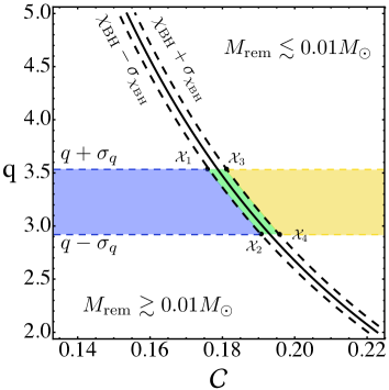
Figure 1: Contour plot of the fit (1) in the $q$-${\cal C}$ plane, for $M_{\textnormal{NS}}=1.2M_{\odot}$, $\chi_{\textnormal{BH}}=0.5$ and $M_{\textnormal{rem}}=0.01M_{\odot}$. The fit separates the region allowed for SGRB ignition (below the fit curve) from the forbidden region (above the fit). Given the measured values of $q\pm\sigma_{q}$ and $\chi_{\textnormal{BH}}\pm\sigma_{\chi_{\textnormal{BH}}}$, a detected signal can correspond to a NS with compactness ${\cal C}$ which falls in the blue, green or yellow region. Since ${\cal C}$ also comes with an error $\sigma_{\cal C}$, in order to infer if it can be associated with a SGRB, we need to evaluate the probability $\textnormal{P}({\cal C}\leq{\cal C}_{4})$ and $\textnormal{P}({\cal C}\leq{\cal C}_{1})$ (see text).

In order to get this information, we need to evaluate ${\cal C}$. As discussed in DNV12 ; DABV13 ; MGF13 ; RMSUCF09 ; Retal13 ; PROR11 , Advanced LIGO/Virgo are expected to measure the gravitational wave phase with an accuracy sufficient to estimate the NS tidal deformability $\lambda_{2}$. Thus, using the fit (3), the NS compactness ${\cal C}_{\lambda}$ and the corresponding uncertainty

$$\sigma_{{\cal C}_{\lambda}}^{2}=\sigma^{2}_{\textnormal{fit}}+\sum_{i,j}\frac{\partial{\cal C}_{\lambda}}{\partial p_{i}}\frac{\partial{\cal C}_{\lambda}}{\partial p_{j}}\textnormal{Cov}(p_{i},p_{j})$$ (4)

can be inferred. In (4) $p_{i}=\{\lambda_{2},M_{\textnormal{NS}}\}$, and $\textnormal{Cov}(p_{i},p_{j})$ is their covariance. As shown in MCFGP13 , $\sigma_{\textnormal{fit}}=0.03\,{\cal C}$ is the largest relative discrepancy between the value of ${\cal C}$ obtained from the fit and the value computed solving the equations of stellar perturbations, for a set of EoS covering a large range of stiffness.

Knowing the parameters and their uncertainties, the probability that a SGRB is associated to the detected coalescence can now be evaluated.

We assume that $(q,\cal{C}_{\lambda},\chi_{\textnormal{{BH}}})$ are described by a multivariate Gaussian distribution:

$${\cal P}(q,{\cal C}_{\lambda},\chi_{\textnormal{BH}})=\frac{1}{(2\pi)^{3/2}|\Sigma|^{1/2}}\textnormal{exp}\left[-\frac{1}{2}\Delta^{\textnormal{T}}\Sigma^{-1}\Delta\right]\ ,$$ (5)

where $\Delta=(\vec{x}-\vec{\mu})$,   $\vec{\mu}=(q,{\cal C}_{\lambda},\chi_{\textnormal{BH}})$,   $\Sigma$ is the covariance matrix. Then, we define the maximum and minimum probability that the binary coalescence produces an accretion disk with mass over the threshold, $\bar{M}_{\textnormal{rem}}$, as

$$\textnormal{P}_{\textnormal{MAX}}(M_{\textnormal{rem}}\gtrsim\bar{M}_{\textnormal{rem}}) \equiv \textnormal{P}({\cal C}_{\lambda}\leq{\cal C}_{4})\ ,$$ (6)

$$\textnormal{P}_{\textnormal{MIN}}(M_{\textnormal{rem}}\gtrsim\bar{M}_{\textnormal{rem}}) \equiv \textnormal{P}({\cal C}_{\lambda}\leq{\cal C}_{1})\ ,$$

where $\textnormal{P}({\cal C}_{\lambda}\leq{\cal C}_{i})$ is the cumulative distribution of Eq. (5), which gives the probability that the measured compactness ${\cal C}_{\lambda}$, estimated through the fit (3), is smaller than an assigned value ${\cal C}_{i}$.

As an illustrative example, we now evaluate the probability that a given BH-NS coalescing binary produces a SGRB, assuming a set of equations of state for the NS matter and evaluating the uncertainties on the relevant parameters using a Fisher matrix approach.

Evaluation of the uncertainties on the binary parameters.—The accuracy with which future interferometers will measure a set of binary parameters $\boldsymbol{\theta}$, is estimated by comparing the gravity-wave data-stream with a set of theoretical templates. For strong enough signals, $\boldsymbol{\theta}$ are expected to have a Gaussian distribution centered around the true values, with covariance matrix

$$\textnormal{Cov}^{ab}=(\Gamma^{-1})^{ab}\qquad\ ,\qquad\Gamma^{ab}=\left(\frac{\partial h}{\partial\theta^{a}}\Bigg{|}\frac{\partial h}{\partial\theta^{b}}\right)\ .$$ (7)

being $\Gamma$ the Fisher information matrix PW95 . $(\cdot|\cdot)$ is the inner product between two GW templates $\tilde{h}(f)$ and $\tilde{g}(f)$:

$$(h|g)=2\int_{f_{\textnormal{min}}}^{f_{\textnormal{max}}}\frac{\tilde{h}(f)\tilde{g}^{\star}(f)+\tilde{h}^{\star}(f)\tilde{g}(f)}{S_{n}(f)}df\ ,$$ (8)

^⋆ denotes complex-conjugation, and $S_{n}(f)$ is the noise spectral density of the considered detector. To model the waveform we use the TaylorF2 approximant in the frequency domain, assuming the stationary phase approximation DIS00 :

$$h(f)={\cal A}(f)e^{i\psi(f)}=\sqrt{\frac{5}{24}}\frac{{\cal M}^{5/6}}{\pi^{2/3}d}f^{-7/6}e^{i\psi(f)}\ .$$ (9)

where $d$ is the source distance. The post-Newtonian expansion of the phase includes spin-orbit and tidal corrections. It can be written as $\psi(f)=\psi_{\textnormal{PP}}+\psi_{\textnormal{T}}$, where the point-particle term is

$$\psi_{\textnormal{PP}}(f)=2\pi t_{c}-\phi_{c}-\frac{\pi}{4}+\frac{3}{128}({\cal M}\pi f)^{-5/3}\sum_{i=0}^{7}e_{i}(m\pi f)^{i/3}\ ,$$ (10)

and $t_{c}$ and $\phi_{c}$ are the time and the phase at coalescence. The coefficient $e_{i}$ are listed in BFIJ02 ; BDE04 . The tidal contribution $\psi_{\textnormal{T}}$ is given by VFH11 ; DNV12

$$\psi_{\textnormal{T}}(f)=- \frac{117\Lambda}{8\nu m^{5}}x^{5/2}\Bigg{[}1+\frac{3115}{1248}x-\pi x^{3/2}\ +$$

$$+\left(\frac{23073805}{3302208}+\frac{20}{81}6\right)x^{2}-\frac{4283}{1092}\pi x^{5/2}\Bigg{]}\ ,$$ (11)

where $x=(m\pi f)^{5/3}$ and $\Lambda$ is the averaged tidal deformability, which for BH-NS binaries reads FH08 : $\Lambda=\lambda_{2}\frac{\left(1+12q\right)}{26}$.

We consider non rotating NSs, as this is believed to be a reliable approximation of real astrophysical systems BC92 ; K92 . The GW waveform is therefore described in terms of the following set of parameters, $\boldsymbol{\theta}=(\ln{\cal A},t_{c},\phi_{c},\ln{\cal M},\ln\nu,\Lambda,\beta)$, where $\beta$ is the 2 PN spin-orbit contribution in $\psi_{\textnormal{PP}}$:

$$\beta=\frac{\chi_{\textnormal{BH}}}{12}\left[113\frac{M_{\textnormal{BH}}^{2}}{m^{2}}+75\nu\right]\hat{\textbf{L}}\cdot\hat{\textbf{S}}_{\textnormal{BH}}\ ,$$ (12)

where $\hat{\textbf{L}}$, $\hat{\textbf{S}}_{\textnormal{NH}}$ are the unit vectors in the direction of the orbital angular momentum and of the spin, respectively. We choose the BH spin aligned with the orbital angular momentum. Moreover, since ${\chi}_{\textnormal{BH}}\leq|1|$, $\beta\lesssim 9.4$; therefore we consider the following prior probability distribution on $\beta$: $p^{(0)}(\beta)\propto\textnormal{exp}\left[-\frac{1}{2}\left(\beta/9.4\right)^{2}\right]\ .$

Thus, we need to compute a $7\times 7$ Fisher matrix. However, since $\ln{\cal A}$ is uncorrelated with the other variables, we perform derivatives only with respect to the remaining six parameters $\boldsymbol{\theta}=(t_{c},\phi_{c},\ln{\cal M},\ln\nu,\Lambda,\beta)$. In our analysis we consider both second (AdvLIGO/Virgo) and third generation (Einstein Telescope, ET, ET1 ) detectors. For AdvLIGO/Virgo we use the ZERO_DET_high_P noise spectral density of AdvLIGO zerodet , in the frequency ranges $[20\ \textnormal{Hz},f_{\textnormal{ISCO}}]$; for the Einstein Telescope we use the analytic fit of the sensitivity curve provided in ET2 , in the range $[10\ \textnormal{Hz},f_{\textnormal{ISCO}}]$. $f_{\textnormal{ISCO}}$ is the frequency of the Kerr ISCO including corrections due to NS self-force Fav11 :

$$f_{\textnormal{ISCO}}=\frac{M_{\textnormal{BH}}}{m\pi}\Omega(\chi_{\textnormal{BH}})\left[1+\nu c^{\textnormal{GSF}}(\chi_{\textnormal{BH}})\right]\ ,$$ (13)

with $\Omega(\chi_{\textnormal{BH}})=\textnormal{sign}(\chi_{\textnormal{BH}})M_{\textnormal{BH}}^{1/2}/(r_{\textnormal{ISCO}}^{3/2}+\chi_{\textnormal{BH}})$.

We model the NS structure by means of piecewise polytropes, RMSUCF09 . The core EoS changes with an overall pressure shift $p_{1}$, specified at the density $\rho_{1}=5.0119\times 10^{14}$g cm^-3. Once the adiabatic index $\Gamma_{\textnormal{core}}$ is fixed, increasing $p_{1}$ produces a family of neutron stars with growing radius for a given mass. Choosing $\Gamma_{\textnormal{core}}=3$ and $p_{1}=(10^{13.95},10^{13.55},10^{13.45},10^{13.35})$ g/cm³ we obtain four EoS, 2H,H, HB and B, which denote very stiff, stiff, moderately stiff and soft EoS, respectively. The stellar parameters for $M_{\textnormal{NS}}=(1.2,1.35)M_{\odot}$, are shown in Table 1.

EoS	$M_{\textnormal{NS}}(M_{\odot})$	${\cal C}$	$\lambda_{\textnormal{2}}$ (km5)	$M_{\textnormal{NS}}(M_{\odot})$	${\cal C}$	$\lambda_{\textnormal{2}}$ (km5)
2H	1.2	0.117	75991	1.35	0.131	72536
H	1.2	0.145	21232	1.35	0.163	18964
HB	1.2	0.153	15090	1.35	0.172	13161
B	1.2	0.162	10627	1.35	0.182	8974

Table 1: For each EoS we show the NS mass, the compactness ${\cal C}=M_{\textnormal{NS}}/R_{\textnormal{NS}}$, and the tidal deformability $\lambda_{2}$.

Numerical results.—Following the strategy previously outlined, we compute the minimum and maximum probabilities (6) that the coalescence of a BH-NS system produces a remnant disk with mass above a threshold $\bar{M}_{\textnormal{rem}}$, for the NS models listed in Table 1 and different values of the mass ratio $q$. The results are given in Table 2, for $q=3$ and $q=7$, black hole spin $\chi_{\textnormal{BH}}=(0.2,0.5,0.9)$, $M_{\textnormal{NS}}=(1.2,1.35)~{}M_{\odot}$, and disk mass thresholds $\bar{M}_{\textnormal{rem}}=0.01M_{\odot}$.

For AdvLIGO/Virgo we put the source at a distance of $100$ Mpc. For ET the binary is at $1$ Gpc. In this case the signal must be suitably redshifted CF94 ; MGF13 , and we have assumed that $z$ is known with a fiducial error of the order of 10% MR12 .

		$q=3$	$d=100$ Mpc	AdV	$q=3$	$d=1$ Gpc	ET	$q=7$	$d=100$ Mpc	AdV	$q=7$	$d=1$ Gpc	ET
	$M_{\textnormal{NS}}=1.2M_{\odot}$		$\chi_{\textnormal{BH}}$			$\chi_{\textnormal{BH}}$			$\chi_{\textnormal{BH}}$			$\chi_{\textnormal{BH}}$
EOS	${\cal C}_{\lambda}$	$0.2$	$0.5$	$0.9$	$0.2$	$0.5$	$0.9$	$0.2$	$0.5$	$0.9$	$0.2$	$0.5$	$0.9$
2H	0.118	1	1	1	1	1	1	0.4	[0.8-0.9]	1	[0.3-0.4]	[0.7-0.8]	1
H	0.147	[0.6-0.9]	1	1	[0.9-1]	1	1	0.4	0.4	[0.8-0.9]	0.3	[0.3-0.4]	1
HB	0.155	[0.5-0.7]	[0.9-1]	1	[0.7-0.8]	1	1	0.4	0.4	[0.7-0.8]	0.3	0.3	0.9
B	0.164	[0.4-0.6]	[0.7-0.8]	1	[0.5-0.6]	1	1	0.4	0.4	[0.6-0.7]	0.3	0.3	[0.7,0.8]
	$M_{\textnormal{NS}}=1.35M_{\odot}$
2H	0.132	1	1	1	1	1	1	0.3	[0.4-0.5]	1	0.2	[0.4,0.5]	1
H	0.164	[0.4-0.6]	[0.8-0.9]	1	[0.4-0.6]	1	1	0.4	0.4	0.7	0.3	0.3	0.8
HB	0.173	[0.4-0.5]	[0.6-0.8]	1	[0.3-0.4]	0.8	1	0.4	0.4	0.6	[0.3-0.4]	[0.3-0.4]	0.6
B	0.184	[0.4-0.5]	[0.5-0.6]	1	[0.3-0.4]	0.6	1	0.4	0.4	0.5	0.4	0.4	[0.5-0.6]

Table 2: We show the probability range [P${}_{\textnormal{MIN}}$,P${}_{\textnormal{MAX}}$] that the coalescence of a BH-NS binary produces a disk mass larger than $\bar{M}_{\textnormal{rem}}=0.01M_{\odot}$ for AdLIGO/Virgo (AdV) and for the Einstein telescope (ET), for binaries with $q=3$ and $q=7$, NS masses (1.2,1.35)$M_{\odot}$, and BH spin $\chi_{\textnormal{BH}}=(0.2,0.5,0.9)$. Sources are assumed to be at $d=100$ Mpc for advanced detectors, and $d=1$ Gpc for the Einstein Telescope. The star compactness ${\cal C}_{\lambda}$ is estimated throughout the universal relation (3).

The first clear result is that as the BH spin approaches the highest value we consider, $\chi_{\textnormal{BH}}=0.9$, and for low mass ratio $q=3$, the probability that a BH-NS coalescence produces a disk with mass above the threshold is insensitive to the NS internal composition, and it approaches unity for all considered configurations. These would be good candidates for GRB production. For the highest mass ratio we consider, $q=7$, the probability to form a sufficiently massive disk depends on the NS mass and EoS, and on the detector. In particular, it decreases as the EoS softens, and as the NS mass increases. This is a general trend, observed also for smaller values of $\chi_{\textnormal{BH}}$. However, when $\chi_{\textnormal{BH}}=0.9$ the probability that the coalescence is associated to a SGRB is always $\gtrsim 50\%$ .

Let us now consider the results for $\chi_{\textnormal{BH}}=0.2$. If the NS mass is $1.2~{}M_{\odot}$ the probability that a detected GW signal from a BH-NS coalescence is associated to the formation of a black hole with a disk of mass above threshold is $\gtrsim 50\%$ for both AdvLIGO/Virgo and ET, provided $q=3$. For larger NS mass, this remains true only if the NS equation of state is stiff (2H or H). High values of $q$ are disfavoured.

When the black hole spin has an intermediate value, say $\chi_{\textnormal{BH}}=0.5$, Table 2 shows that, the NS compactness plays a key role in the identification of good candidates for GRB production, for both detectors. Again large values of the mass ratio yield small probabilities.

The range of compactness shown in Table 2 includes neutron stars with radius ranging within $\sim[10,15]$ km. From the table it is also clear that if we choose a compactness smaller than the minimum value, the probability of generating a SGBR increases, and the inverse is true if we consider compactness larger than our maximum.

Concluding remarks.—

The method developed in this paper can be used in several different ways. In the future, gravitational wave detectors are expected to reach a sensitivity sufficient to extract the parameters on which our analysis is based, i.e. chirp mass, mass ratio, source distance, spin and tidal deformability. We can also expect that the steady improvement of the efficiency of computational facilities experienced in recent years will continue, reducing the time needed to obtain these parameters from a detected signal. Moreover, the higher sensitivity will allow to detect sources in a much larger volume space, thus increasing the detection rates. In this perspective, the method we envisage in this paper will be useful to trigger the electromagnetic follow-up of a GW detection, searching for the afterglow emission of a SGRBs.

Waiting for the future, the method we propose can be used in the data analysis of advanced detectors as follows:

• Table II indicates the systems which are more likely to produce accretion disks sufficiently massive to generate a SGRB. The table can be enriched including more NS equations of state or more binary parameters; however, it already contains a clear information on which is the range of parameters to be used in the GW data analysis, if the goal is to search for BH-NS signals which may be associated to a GRB. For instance, Table II suggests that searching for mass ratio smaller than, or equal to, 3-4, and values of the black hole angular momentum larger than 0.5-0.6 would allow to save time and computational resources in low latency search. In addition, it would allow to gain sensitivity in externally triggered searches performed in time coincidence with short GRBs observed by gamma-ray satellites.

• If a SGRB is observed sufficiently close to us in the electromagnetic waveband, the parameters of the GW signal detected in coincidence would allow to set a threshold on the mass of the accretion disk. If the GW signal comes, say, from a system with a BH with spin $\chi_{\textnormal{BH}}=0.5$, mass ratio $q=7$, and neutron star mass $M_{\textnormal{NS}}=1.2M_{\odot}$, from Table 2, equations of state softer than the EoS 2H would be disfavoured. Thus, we would be able to shed light on the dynamics of the binary system, on its parameters and on the internal structure of its components. We would enter into the realm of gravitational wave astronomy.

Finally, it is worth stressing that as soon as the fit (1) will be extended to NS-NS coalescing binaries, this information will be easily implemented in our approach. Being the rate of NS-NS coalescence higher than that of BH-NS, our approach will acquire more significance, and will be a very useful tool to study these systems.

Acknowledgements.—We would like to thank M. Branchesi for her comments on the paper, which helped us to clarify several issues. We would like to thank L. Pagano, R. Amato and M. Muccino for useful discussions and comments. A. M. is supported by a ”Virgo EGO Scientific Forum” (VESF) grant. Partial support comes from the CompStar network, COST Action MP1304.

References

- (1) http://www.ligo.caltech.edu, http://www.ego-gw.it.
- (2) William H. Lee and Enrico Ramirez-Ruiz, New J. Phys. 9, 17 (2007).
- (3) J. Abadie et al. [LIGO Scientific Collaboration], Astrophys. J. 755 (2012) 2.
- (4) J. Abadie et al. [LIGO Scientific Collaboration], Astrophys. J. 760 (2012) 12.
- (5) J. Aasi et al., arXiv:1304.0670 (2013).
- (6) J. Abadie et al. [LIGO Scientific Collaboration], A&A 541 A155 (2012).
- (7) Francois Foucart, Phys. Rev. D 86, 124007 (2012).
- (8) B. Giacomazzo, R. Perna, L. Rezzolla, E. Troja and D. Lazzati, The Astrophysical Journal Letters, 762:L18, (2013).
- (9) J. M. Bardeem, W. H. Press and S. A. Teukolsky, Astrophys. J. 178, 347 (1972).
- (10) K. Kyutoku, H. Okawa, M. Shibata, K. Taniguchi, Phys. Rev. D 84, 064018 (2011).
- (11) Z.B. Etienne, Y.T. Liu, S.L. Shapiro and T.W. Baumgarte, Phys. Rev. D 79, 044024 (2009).
- (12) F. Foucart, M.D. Duez, L.E. Kidder, M.A.Scheel, B. Szilagyi, S.A. Teukolsky, Phys. Rev. D 85, 044015 (2012).
- (13) F. Foucart, M.D. Duez, L.E. Kidder, S.A. Teukolsky, Phys. Rev. D 83, 024005 (2011).
- (14) T. Piran, Rev. Mod. Phys. 76, 1143 (2004).
- (15) S. Setiawan, M. Ruffert and H. -T. Janka, Mon. Not. Roy. Astron. Soc. 352, 753 (2004).
- (16) T. D. Matteo, R. Perna and R. Narayan, Astrophys. J. 579, 706 (2002).
- (17) R. Popham, S. E. Woosley and C. Fryer, Astrophys. J. 518, 356 (1999).
- (18) A. Maselli, V. Cardoso, V. Ferrari, L. Gualtieri and P. Pani, Phys. Rev. D 88, 023007 (2013).
- (19) W. Del Pozzo, T. G. F. Li, M. Agathos, C. V. D. Broeck and S. Vitale, Phys. Rev. Lett. 111, 071101 (2013).
- (20) T. Damour, A. Nagar, L. Villain, Phys. Rev. D 85, 123007 (2012).
- (21) J. Read, et al., Phys. Rev. D 88, 044042 (2013).
- (22) F. Pannarale, L. Rezzolla, F. Ohme, J. S. Read, Phys. Rev. D 84, 104017 (2011).
- (23) A. Maselli, L. Gualtieri, V.Ferrari, Phys. Rev. D 88, 104040 (2013).
- (24) J. Read, et al., Phys. Rev. D 79, 124033 (2009).
- (25) E. Poisson and C. M. Will, Phys. Rev. D 52, 2 (1995).
- (26) T. Damour, B. Iyer, B. Sathyaprakash, Phys. Rev. D 62 084036 (2000).
- (27) L. Blanchet, G. Faye, B. R. Iyer and B. Jouget, Phys. Rev. D 65, 061501 (2004).
- (28) L. Blanchet, T. Damour, G. Esposito Farese and B. R. Iyer, Phys. Rev. Lett. 93, 091011 (2004).
- (29) J. Vines, E.E. Flanagan, T. Hinderer, Phys. Rev. D 83, 084051 (2011).
- (30) E.E. Flanagan, T. Hinderer, Phys. Rev. D 77, 021502 (2008).
- (31) L. Bildsten and C. Cutler, Astroph. J 400, 175 (1992).
- (32) C. S. Kochanek, Astroph. J 398, 234 (1992).
- (33) http://www.et-gw.eu
-
(34)
D. Shoemaker, https://dcc.ligo.org/cgi-bin/DocDB/
ShowDocument?docid=2974. - (35) B.S. Sathyaprakash and B.F. Schultz, Living Rev. Relativity 12, 2 (2009).
- (36) Marc Favata, Phys. Rev. D 83, 024028 (2011).
- (37) C. Cutler and E. E. Flanagan, Phys. Rev. D 49 (1994) 2658.
- (38) C. Messenger and J. Read, Phys. Rev. Lett. 108 (2012) 09110.