Abstract

We derive the complete factorization formula for the leading power contribution in wide angle Compton scattering. It consists of the soft- and hard-spectator contributions. The hard-spectator contribution is well known and defined in the form of the convolution of a hard kernel with the nucleon distribution amplitudes. The soft-spectator contribution describes the scattering which involves the soft modes. We use the soft collinear effective theory in order to define this term in a field theoretical approach. Using the SCET framework we provide the proof of the factorization formula. We also compute the next-to-leading QCD corrections to the hard coefficient function of the soft spectator contribution and perform a phenomenological analysis of existing experimental data within the developed formalism.

Introduction

The Wide Angle Compton scattering (WACS) provides an excellent possibility to study the complicated hadronic dynamics in hard exclusive processes. The asymptotic behavior of the cross section for this process at large energy and momentum transfer $s\sim-t\sim-u\gg\Lambda$, where $\Lambda$ is the typical hadronic scale, was predicted long time ago using the QCD power counting arguments [1, 2]. It was suggested that

$$\frac{d\sigma^{\gamma p\rightarrow\gamma p}}{dt}\sim\frac{1}{s^{6}}f(\theta),$$ (1)

where $\theta$ denotes the scattering angle in the center-of-mass frame. Later the QCD factorization approach was developed in order to compute the function $f(\theta)$, see e.g. Refs.[3, 4] . The asymptotic expression for this function is dominated by the hard two-gluon exchange diagrams. The non-perturbative dynamics in this case is described by the so-called nucleon distribution amplitude (DA) which is related with the three-quark Fock component of the nucleon wave function in the light-cone formalism [5].

The first measurements of the differential cross section were carried out in a Cornell experiment [6]. It was found that the cross section displays a scaling behavior which is in a reasonable agreement with pQCD predictions (1). However theoretical estimates show that the absolute value of the cross section computed within the QCD factorization framework is much smaller than the corresponding experimental values [7, 8, 9, 10]. The new experiments carried out at JLab for large angle scattering provided more precise data for the cross section for the different energies [11]. The new data have much better accuracy and allow one to carry a more detailed comparison with the theoretical predictions for the cross section. Moreover, for the first time the longitudinal and transverse components of the recoil proton polarization were also measured [12]. These measurements provided that the value of the longitudinal asymmetry $K_{\text{LL}}$ is qualitatively different from the one that can be obtained in the hard-spectator (hard two-gluon exchange) factorization picture described above.

All these observations indicate that the existing data are still far away from the asymptotic region where the formula (1) based on the hard two-gluon exchange is dominant. Therefore in order to explain the confrontation of the theory with the data one has to implement a different picture of the scattering which describes also the dominant preasymptotic effects. To this extent, promising results have been obtained within the hand-bag model approach [13, 14, 15, 16]. The main idea of this model is that the dominant contribution in the relevant kinematical region is provided by the soft-overlap contribution which is also known as the Feynman mechanism. In this model both photons interact with a single quark which couples to the soft spectators through the generalized parton distributions (GPDs). The GPDs describe the nonperturbative soft-overlap mechanism at small momentum transfer $-t\sim\Lambda^{2}$ and their models can be constrained by using their relations to the form factors and usual parton distributions, see e.g. [17, 18, 19] and references therein. The extension of the GPD formalism for the description of the region with large $-t\gg\Lambda$ is the key assumption of the handbag model. There is also an alternative approach based on the constituent quark model [20]. All these models provide a satisfactory description of the cross section data and asymmetry $K_{\text{LL}}$ that demonstrates a strong support for the crucial role played by the soft-spectator scattering in WACS and possibly in other hard reactions.

The further and more accurate experimental studies of the WACS cross sections and asymmetries can be performed at JLab after the 12 GeV Upgrade [21]. This provides a strong motivation to develop a systematic theoretical approach which accommodates consistently both hard- and soft-spectator reaction mechanisms and allows one to reduce the model dependence in the data analysis.

Some steps in this direction were made in the framework of the GPD handbag model in Refs.[18, 22]. However in the latter framework one is faced with the problem how to consistently perform the matching between the hard and the soft regions: it is not clear how to map systematically the infrared poles arising from the partonic diagrams with the ultraviolet structure of the GPD-based matrix elements. This difficulty does not allow to formulate a consistent theoretical approach.

The importance of the soft modes and their specific role for the description of hard processes with nucleons has already been observed a long time ago in Refs. [23, 24]. A substantial progress in the theoretical description of such configurations has been achieved during past decade in the framework of the soft collinear effective theory (SCET) [25, 26, 27, 28, 29, 30]. An application of this technique for the description of the soft-overlap contribution in different hadronic hard exclusive reactions including WACS has recently been studied in Refs.[34, 35, 36, 37]. The attractive feature of this approach is the possibility to formulate the factorization of the hard- and the soft-spectator contributions consistently using a field theory technique. This can be done because of the presence of the collinear and soft modes in the effective Lagrangian. This allows one to establish a systematic power counting rule for all contributions which can be relevant for a given process, and to include the hard- and soft-spectator configurations on the same footing .

The soft modes in the SCET approach describe particles with the momenta $k_{s}^{\mu}\sim\Lambda$. The presence of such modes unavoidably introduces the additional intermediate scale of order $\Lambda Q$ which is known as a hard-collinear scale. Such intermediate virtualities naturally arises due to the interactions between the collinear and soft particles. In such case the factorization of an amplitude can be described in terms of the two following steps. In a first step one integrates out the hard modes describing the particles with momenta $p_{h}^{\mu}\sim Q$. The remaining relevant degrees of freedom are then described by the hard-collinear, collinear and soft particles. If the value of the hard scale $Q$ is quite large so that the hard-collinear scale $\mu_{hc}\sim\sqrt{\Lambda Q}$ is also quite large, then one can proceed further and to integrate over the hard-collinear modes. After that the unknown nonperturbative dynamics is described by matrix elements of the operators constructed only from collinear or soft fields. In case the hard-collinear scale is not large, for instance $\mu_{hc}\lesssim 1$GeV then only the first step factorization can be performed. Notice that such a framework provides a clear theoretical understanding of the intermediate region of $Q^{2}$. Namely, this region can be associated with the values of $Q^{2}$ for which the hard-collinear scale is not large enough and the full two-step factorization description can not provide an accurate description. It seems that this situation is relevant in the description of many hard exclusive processes including also WACS which is the subject of this paper.

The complete QCD factorization formula which includes the hard- and soft-spectator contributions for WACS has been suggested in Ref.[36]. It was shown there that the soft-spectator configuration in WACS and elastic electron-proton scattering is described by the same matrix element and this allows to constrain a particular contribution entering the two-photon exchange amplitudes. However in Ref.[36] the factorization for Compton scattering was not discussed in detail. In the current publication we provide the details of this formalism. We provide the proof of the factorization formula within the SCET framework and also compute the next-to-leading hard corrections to coefficient functions in front of the SCET operator which describe the soft-spectator contribution. Then we use the obtained results in the phenomenological analysis of existing data.

Our paper is organized as follows. In Section 1 we discuss the general properties of the WACS. We specify notations and kinematics, discuss the amplitude and cross section. In the Section 2 we discuss the QCD factorization of the WACS amplitudes within the SCET framework. We prove that the complete factorization formula consists of two contributions associated with the soft- and hard-spectator scattering and provide their theoretical description. Section 3 is devoted to the calculation of the next-to-leading order coefficient functions for the soft-spectator contribution. In Section 4 we use the obtained expressions for the analysis of existing experimental data. In Appendix we present more details about the next-to-leading calculations.

1 Wide angle Compton scattering: general remarks

The kinematics of the real Compton scattering $\gamma(q)+N(p)\rightarrow\gamma(q^{\prime})+N(p^{\prime})$ is described by the Mandelstam variables

$$s=(p+q)^{2},\quad t=(p^{\prime}-p)^{2}<0,\quad u=(p-q^{\prime})^{2}<0,\quad s+t+u=2m^{2}.$$ (2)

In the center-of-mass frame $\vec{p}+\vec{q}=0$ the particle momenta read

$$p=E_{cm}\left(\sqrt{1+\frac{m^{2}}{E_{cm}^{2}}},0,0,-1\right),~{}\ q=E_{cm}(1,0,0,1),$$ (3)

$$p^{\prime}=E_{cm}\left(\sqrt{1+\frac{m^{2}}{E^{2}}},-\sin\theta,0,-\cos\theta\right),~{}\ q^{\prime}=E_{cm}(1,\sin\theta,0,\cos\theta),$$ (4)

where $m$ denotes the nucleon mass and $\theta$ is the scattering angle in the center-of-mass frame.

In what follows, we will also use the auxiliary light-cone vectors $n,\ \bar{n}$ such that

$$n=(1,0,0,-1),~{}\bar{n}=(1,0,0,1),~{}\ (n\cdot\bar{n})=2.$$ (5)

In order to write the light-cone expansions of the particle momenta we choose a frame where $z$-axis is directed along the incoming and outgoing nucleons. For large-angle kinematics $s\sim-t\sim-u\gg m^{2}\sim\Lambda^{2}$ one obtains

$$p = \sqrt{-t}\frac{\bar{n}}{2}+\frac{m^{2}}{\sqrt{-t}}\frac{n}{2}\simeq\sqrt{-t}\frac{\bar{n}}{2},\quad p^{\prime}=\frac{m^{2}}{\sqrt{-t}}\frac{\bar{n}}{2}+\sqrt{-t}\frac{n}{2}\simeq\sqrt{-t}\frac{n}{2},,$$ (6)

$$q \simeq \frac{u}{t}\ p-\frac{s}{t}\ p^{\prime}+q_{\bot},~{}\ q^{\prime}\simeq-\frac{s}{t}\ p+\frac{u}{t}\ p^{\prime}+q_{\bot},$$ (7)

where we neglected the power corrections $m/Q$ and assume $-t\simeq\frac{1}{2}s(1-\cos\theta)$, $-u\simeq\frac{1}{2}s(1+\cos\theta)$.

In order to describe the amplitude of the Compton scattering it is convenient to introduce the following notations [38]

$$P=\frac{1}{2}(p+p^{\prime}),~{}K=\frac{1}{2}(q+q^{\prime}),~{}P^{\prime}=P-K\frac{(P\cdot K)}{K^{2}},$$ (8)

$$N_{\mu}=\varepsilon_{\mu\alpha\beta\gamma}P^{\alpha}\frac{1}{2}(p-p^{\prime})^{\beta}K^{\gamma},~{}\ \varepsilon_{0123}=+1,$$ (9)

Then the real Compton amplitude on the proton can be described in terms of six scalar amplitudes $T_{i}(s,t)$

$$\langle p^{\prime},q^{\prime};out|S-1|in;p,q\rangle=i(2\pi)^{4}\delta(p^{\prime}+q^{\prime}-p-q)M^{\gamma p\rightarrow\gamma p}.$$ (10)

with

$$M^{\gamma p\rightarrow\gamma p} = -e^{2}\,\varepsilon^{\ast\mu}(q^{\prime})\varepsilon^{\nu}(q)\bar{N}(p^{\prime})\left\{-\mathcal{T}_{12}^{\mu\nu}\left(T_{1}+K\hskip-7.0pt/~{}T_{2}\right)-\mathcal{T}_{34}^{\mu\nu}\left(T_{3}+K\hskip-7.0pt/~{}T_{4}\right)\right.$$ (11)

$$\left.\phantom{\varepsilon^{\ast\mu}(q^{\prime})\varepsilon^{\nu}(q)\bar{N}(p^{\prime})\{-\mathcal{T}_{12}}+\mathcal{T}_{5}^{\mu\nu}i\gamma_{5}~{}T_{5}+\mathcal{T}_{6}^{\mu\nu}~{}i\gamma_{5}K\hskip-7.0pt/~{}T_{6}\right\}N(p),$$

where $e$ denotes the electromagnetic charge of the proton. In Eq.(11) we introduced the following tensor structures

$$\mathcal{T}_{12}^{\mu\nu}=-\frac{P^{\prime\mu}P^{\prime\nu}}{P^{\prime 2}},\quad\mathcal{T}_{34}^{\mu\nu}=\frac{N^{\mu}N^{\nu}}{N^{2}},\quad\mathcal{T}_{5}^{\mu\nu}=\frac{P^{\prime\mu}N^{\nu}-P^{\prime\nu}N^{\mu}}{P^{\prime 2}K^{2}},\quad\mathcal{T}_{6}^{\mu\nu}=\frac{P^{\prime\mu}N^{\nu}+P^{\prime\nu}N^{\mu}}{P^{\prime 2}K^{2}}.$$ (12)

One can easily see that the tensor $\mathcal{T}_{j\ \mu\nu}$ are gauge invariant and orthogonal

$$q^{\nu}\mathcal{T}_{j\ \mu\nu}=q^{\prime\mu}\mathcal{T}_{j\ \mu\nu}=0,\quad\mathcal{T}_{i}^{\mu\nu}\mathcal{T}_{j\ \mu\nu}=0,\quad i\neq j,$$ (13)

$$\mathcal{T}_{12}^{\mu\nu}\mathcal{T}_{12\mu\nu}=\mathcal{T}_{34}^{\mu\nu}\mathcal{T}_{34\mu\nu}=1,\quad\mathcal{T}_{5}^{\mu\nu}\mathcal{T}_{5\mu\nu}=\mathcal{T}_{6}^{\mu\nu}\mathcal{T}_{6\mu\nu}=2.$$ (14)

This allows one to compute the contribution to a given amplitude using appropriate contractions.

The unpolarized differential cross section describing real Compton scattering reads [38]

$$\frac{d\sigma}{dt} = \frac{\pi\alpha^{2}}{(s-m^{2})^{2}}\left\{(s-m^{2})(m^{2}-u)\frac{1}{2}(|T_{2}|^{2}+|T_{4}|^{2})+(m^{4}-su)|T_{6}|^{2}\right.$$ (15)

$$\left.+m(s-u)\operatorname{Re}\left[T_{1}T_{2}^{\ast}+T_{3}T_{4}^{\ast}\right]+\frac{1}{2}(4m^{2}-t)(|T_{1}|^{2}+|T_{3}|^{2})-t|T_{5}|^{2}\right\},$$

where the fine structure coupling $\alpha=e^{2}/4\pi\simeq 1/137$. The explicit expressions for the observables including the longitudinal polarization $K_{\text{LL}}$ can also be found in Ref.[38] and we will not rewrite it here.

2 QCD factorization for wide angle Compton scattering within the SCET framework

2.1 SCET: preliminary remarks

In this section we consider in detail the leading power factorization of the WACS amplitudes using the SCET approach developed in Refs.[25, 26, 27, 28, 29, 30]. Below we assume that the relevant dominant regions are described by particles which have hard $p_{h}$, hard-collinear $p_{hc}$, collinear $p_{c}$ and soft $p_{s}$ momenta. The light-cone components $\left(p\cdot n,p\cdot\bar{n},p_{\bot}\right)\equiv(p_{+},p_{-},p_{\bot})$ of the corresponding momenta scale as

$$p_{h}\sim Q\left(1,1,1\right),~{}p_{h}^{2}\sim Q^{2},$$ (16)

$$p_{hc}\sim Q\left(1,\lambda^{2},\lambda\right)\text{ or }p_{hc}^{\prime}\sim Q\left(\lambda^{2},1,\lambda\right),~{}p_{hc}^{2}\sim Q^{2}\lambda^{2}\ \sim Q\Lambda,$$ (17)

$$p_{c}\sim Q\left(1,\lambda^{4},\lambda^{2}\right)\text{ or ~{}}p_{c}^{\prime}\sim Q\left(\lambda^{4},1,\lambda^{2}\right),~{}\ p_{c}^{2}\sim Q^{2}\lambda^{4}\sim\Lambda^{2},$$ (18)

$$p_{s}\sim Q\left(\lambda^{2},\lambda^{2},\lambda^{2}\right),~{}\ p_{s}^{2}\sim Q^{2}\lambda^{4}\sim\Lambda^{2}.$$ (19)

The scales $Q$ and $\Lambda$ denote the generic large and soft scales, respectively. The small dimensionless parameter $\lambda$ is set to be $\lambda\sim\sqrt{\Lambda/Q}$. Let us assume that there are no other relevant modes required for the factorization of the leading power amplitudes. In this case the factorization can be described in two steps: first, we integrate out the hard modes and reduce the full QCD to the effective theory. The corresponding effective Lagrangian is constructed from the hard-collinear and soft particles. This effective theory is denoted as SCET-I. If the hard scale $Q$ is so large that the hard collinear scale $\mu_{hc}\sim\sqrt{Q\Lambda}$ is a good parameter for the perturbative expansion then one can perform the second matching step and to integrate out the hard-collinear modes. Then the resulting effective Lagrangian is constructed only from the collinear and soft fields and the corresponding effective theory is denoted as SCET-II.

For the SCET fields we use the following notations. The fields $\xi_{n}^{C},$ $A_{\mu C}^{(n)}$ and $\xi_{\bar{n}}^{C},~{}A_{\mu C}^{(\bar{n})}~{}$ denote the hard-collinear ($C=hc$) or collinear ($C=c$) quark and gluon fields associated with momentum $p^{\prime}$ and $p$, respectively, see Eq.(6). As usually, the hard-collinear and collinear quark fields satisfy

$$n\hskip-5.5pt/\xi_{n}^{C}=0,~{}~{}\bar{n}\hskip-5.5pt/\xi_{\bar{n}}^{C}=0.$$ (20)

The fields $q$ and $A_{\mu}^{(s)}$ denote the soft quarks and gluons with the soft momenta as in Eq.(19) which also enter in the SCET Lagrangian.

In the wide-angle kinematics we have the energetic particles propagating with large energies in four directions. Therefore it is useful to introduce two more auxiliary light-cone vectors associated with the photon momenta $q$ and $q^{\prime}$

$$\bar{v}^{\mu}=\frac{2q^{\mu}}{\sqrt{-t}},~{}\ v^{\mu}=\frac{2q^{\prime\mu}}{\sqrt{-t}},~{}(\bar{v}\cdot v)=2.$$ (21)

Using the vectors $\bar{v},v$ we also introduce the hard-collinear quark and gluon fields in the similar way as before just changing $(n,\bar{n})\rightarrow\left(v,\bar{v}\right)$.

The explicit expression for the SCET-I  Largangian in position space was derived in Refs.[29, 30]. This Lagrangian can be represented in the form of expansion with respect to the small parameter $\lambda$

$$\mathcal{L}_{\text{SCET}}^{(n)}=\mathcal{L}_{\xi\xi}^{(0,n)}+\mathcal{L}_{\xi\xi}^{(1,n)}+\mathcal{L}_{\xi q}^{(1,n)}+\mathcal{O}(\lambda^{2}),$$ (22)

where $\mathcal{L}^{(\lambda,n)}\sim\mathcal{O}(\lambda)$. The explicit expressions for the simplest terms read

$$\mathcal{L}_{\xi\xi}^{(0,n)}=\bar{\xi}_{n}^{hc}(x)\left(i~{}n\cdot D+gn\cdot A^{(s)}(x_{-})+iD\hskip-7.0pt/_{\bot}\frac{1}{i\bar{n}\cdot D}iD\hskip-7.0pt/_{\bot}\right)\frac{\bar{n}}{2}\xi_{n}^{hc}(x),$$ (23)

$$\mathcal{L}_{\xi q}^{(1,n)}=\bar{\xi}_{n}^{hc}(x)iD\hskip-7.0pt/_{\bot}W_{n}~{}q(x_{-})+\bar{q}(x_{-})W_{n}^{{\dagger}}iD\hskip-7.0pt/_{\bot}\xi_{n}^{hc}(x).$$ (24)

The expression for the subleading term $\mathcal{L}_{\xi\xi}^{(1,n)}$ is a bit lengthy and we will not rewrite it here. The similar expressions are also valid for the other collinear sectors associated with the directions $\bar{n},v,\bar{v}$. In the above formulas we used $iD_{\mu}=i\partial_{\mu}+gA_{\mu hc}^{(n)}$, $x_{-}=\frac{1}{2}(x\cdot\bar{n})n$ and the hard-collinear Wilson lines

$$W_{n}(z)=\text{P}\exp\left\{ig\int_{-\infty}^{0}ds~{}\bar{n}\cdot A_{hc}^{(n)}(z+s\bar{n})\right\}.$$ (25)

The matching from SCET-I to SCET-II can be performed by integration over the hard-collinear fields. Technically this can be done via the substitutions $\xi_{n}^{hc}\rightarrow\xi_{n}^{c}+\xi_{n}^{hc}$ and $A_{hc}^{(n)}\rightarrow A_{c}^{(n)}+A_{hc}^{(n)}$ in the Lagrangian (22) and the external SCET-I operators and integration over the hard-collinear fields. Following this way one has to deal with the intermediate theory which includes the hard-collinear, collinear and soft fields. A more detailed description of this step can be found in Refs.[31, 32] in the hybrid formulation and in Ref.[33] in the position space formulation.

The power counting rules can be fixed using the power counting of the SCET fields. These rules for the SCET fields can be obtained from the corresponding propagators in momentum space and read (see, for instance, Ref.[29])

$$\xi_{n}^{hc}\sim\lambda,~{}\ \bar{n}\cdot A_{hc}^{(n)}\sim 1,~{}A_{\bot hc}^{(n)}\sim\lambda~{}\ ,n\cdot A_{hc}^{(n)}\sim\lambda^{2},$$ (26)

$$\xi_{n}^{c}\sim\lambda^{2},~{}\ \bar{n}\cdot A_{c}^{(n)}\sim 1,~{}A_{\bot c}^{(n)}\sim\lambda^{2}~{}\ ,n\cdot A_{c}^{(n)}\sim\lambda^{4},$$ (27)

$$A_{s}^{\mu}\sim\lambda^{2},~{}\ q\sim\lambda^{3}.$$ (28)

Performing the matching from QCD to SCET-I one has to consider different operators built from the SCET-I fields. It is convenient to construct such operators using the following gauge invariant combinations

$$\chi_{n}^{hc}(\lambda\bar{n})\equiv~{}W_{n}^{{\dagger}}(\lambda\bar{n})\xi_{n}^{hc}(\lambda\bar{n}),~{}\ \bar{\chi}_{n}^{hc}(\lambda\bar{n})\equiv\bar{\xi}_{n}^{hc}(\lambda\bar{n})W_{n}(\lambda\bar{n}),$$ (29)

$$\mathcal{A}_{\mu\ hc}^{(n)}(\lambda\bar{n})\equiv\left[W_{n}^{{\dagger}}(\lambda\bar{n})D_{\mu}W_{n}(\lambda\bar{n})\right],$$ (30)

where the covariant derivative $D_{\mu}$ is applied only inside the brackets. For collinear operators one can use similar expressions.

2.2 Factorization for the WACS amplitudes

The factorization formula for the WACS amplitudes can be written as a sum of two contributions describing the soft- and the hard-spectator scattering. The hard-spectator scattering contribution dominates at asymptotically large values of $Q\rightarrow\infty$. But for the moderate values of $Q$, where the hard-collinear virtualities $Q\Lambda\lesssim m^{2}$ are not large, one has to take into account the soft-overlap contribution which, in general, is described by the matrix elements of the all appropriate SCET-I operators.

Below we show that the complete leading power factorization formula can be written as

$$T_{i}(s,t)=C_{i}(s,t)\mathcal{F}_{1}(t)+\mathbf{\Psi}\ast H_{i}(s,t)\ast\ \mathbf{\Psi},\quad i=2,3,4.$$ (31)

Here the first term describes the soft-spectator contribution while the second term corresponds to the well known hard-spectator mechanism. For illustration, in Fig.1 we show the different contributions in Eq.(31) as appropriate reduced diagrams. In the large $Q$ limit both contributions in Eq.(31) behave as $Q^{-4}$ up to logarithmic corrections and give

$$T_{2,4,6}(s,t)\sim Q^{-4},\quad Q\rightarrow\infty.$$ (32)

For large values of $Q$ the soft-spectator scattering is strongly suppressed due to the so-called Sudakov logarithms and therefore the hard-spectator contribution becomes dominant. But for moderate values of $Q$ the effect of the Sudakov suppression is still weak, see e.g. discussion in Ref.[35], therefore the soft-spectator contribution is quite large or even dominant.

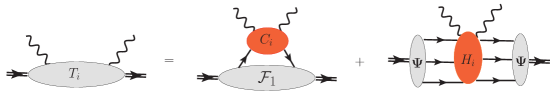
Figure 1: The reduced diagrams describing the factorization formula in Eq.(31).

The expression in Eq.(31) does not include the amplitudes $T_{1,3,5}$. These amplitudes describe the scattering when the helicity of nucleon is not conserved. These amplitudes are suppressed as $\mathcal{O}(1/Q^{5})$ and their factorization is described by the subleading operators in SCET. Therefore we postpone the study of these contributions to future publications.

The asterisks in Eq.(31) denote the convolution with respect to the collinear quark fractions. The non-perturbative dynamics in the hard-spectator contributions is described by nucleon distribution amplitudes $\mathbf{\Psi}$ which are defined by the following matrix elements

$$~{}4\left\langle 0\left|[\chi_{\bar{n}}^{c}]^{i}_{\alpha}(\lambda_{1}n)~{}[\chi_{\bar{n}}^{c}]^{j}_{\beta}(\lambda_{2}n)~{}[\chi_{\bar{n}}^{c}]^{k}_{\sigma}(\lambda_{3}n)\right|p\right\rangle=\frac{\varepsilon^{ijk}}{3!}\int Dx_{i}~{}e^{-ip_{+}\left(\sum x_{i}\lambda_{i}\right)}\mathbf{\Psi}(x_{i}),$$ (33)

where $p_{+}\equiv(p\cdot n)$,

$$[\chi_{\bar{n}}^{c}]^{i}_{\alpha}(z)\equiv\text{P}\exp\left\{ig\int_{-\infty}^{0}dt~{}(n\cdot A_{c})(z+tn)\right\}\left[\xi_{\bar{n}}^{c}\right]_{\alpha}^{i}(z).$$ (34)

Here the indices $i$ and $\alpha$ describe the color and Dirac indices, respectively. The measure in Eq.(33) reads $Dx_{i}=dx_{1}dx_{2}dx_{3}\delta(1-x_{1}-x_{2}-x_{3}).$ The function $\mathbf{\Psi}(x_{i})$ can be rewritten in terms of the three scalar amplitudes $V,A$ and $T$ [4]

$$\mathbf{\Psi}(x_{i}) =V(x_{i})p_{+}\left[\frac{1}{2}\bar{n}\hskip-5.0pt/C\right]_{\alpha\beta}\left[\gamma_{5}N_{\bar{n}}\right]_{\sigma}+A(x_{i})p_{+}\left[{\frac{1}{2}}\bar{n}\hskip-5.0pt/\gamma_{5}C\right]_{\alpha\beta}\left[N_{\bar{n}}\right]_{\sigma}+T(x_{i})p_{+}\left[\frac{1}{2}\bar{n}\hskip-5.0pt/\gamma_{\bot}~{}C\right]_{\alpha\beta}\left[\gamma^{\bot}\gamma_{5}N_{\bar{n}}\right]_{\sigma},$$ (35)

Here the large component $N_{\bar{n}}$ of the nucleon spinor is defined as

$$N_{\bar{n}}=\frac{\bar{n}\hskip-5.0pt/n\hskip-5.0pt/}{4}N(p),$$ (36)

and $C$ is charge conjugation matrix. For simplicity we do not show in Eq.(33) the flavor indices.

The hard coefficient functions $H_{i}(s,t)$ in Eq.(31) define the full dependence of the hard-spectator contribution on the Mandelstam variables. The leading-order approximation for these functions are defined by the two-gluon exchange diagrams and therefore they are of order $\alpha^{2}_{s}(Q^{2})$.

The non-perturbative dynamics in the soft-spectator contribution in Eq.(31) is described by the SCET form factor (FF) $\mathcal{F}_{1}(t)$. In the SCET framework it is defined as

$$\left\langle p^{\prime}\right|O^{\sigma}\left|p\right\rangle_{\text{{\tiny SCET}}}=\bar{N}_{n}\gamma_{\bot}^{\sigma}N_{\bar{n}}~{}\mathcal{F}_{1}(t),$$ (37)

with the operator

$$O^{\sigma}=\sum e_{q}^{2}\left\{\bar{\chi}_{n}^{hc}\gamma_{\bot}^{\sigma}\chi_{\bar{n}}^{hc}-\bar{\chi}_{\bar{n}}^{hc}\gamma_{\bot}^{\sigma}\chi_{n}^{hc}\right\},$$ (38)

where the hard-collinear quark fields in the brackets $\{...\}$ have an appropriate flavor. This SCET FF depends only from the large momentum transfer $t$. However this dependence is associated only with the hard-collinear modes which can not be factorized for small values of the hard-collinear scale. One can see from Eq.(31) that the energy ($s$) dependence is completely defined by the hard coefficient function $C_{i}$ and therefore can be computed in the perturbation theory.

The factorization formula in Eq.(31) does not include the contribution of the gluon SCET operator which is of the same order $\mathcal{O}(\lambda^{2})$ as the quark operator $O^{\sigma}$. In the next section we provide a more detailed explanation of this fact.

The FF $\mathcal{F}_{1}(t)$ and the hard coefficient functions $C_{i}$ also depend on the factorization scale $\mu_{F}$ which is not shown for simplicity. This scale defines the separation between the hard and hard-collinear regions. This scale dependence can be computed from the renormalization of the operator $O^{\sigma}$ (38) in SCET. This provides a possibility for systematic calculations of the higher order corrections associated with the hard region.

Performing the further factorization at very large $Q$ one can show that the SCET FF $\mathcal{F}_{1}(t)$ decreases with the same power as the hard spectator contribution [34]

$$\mathcal{F}_{1}(t)\sim(-t)^{-2}.$$ (39)

However there is one more subtlety which is hidden in the formal definitions and related to the separation of the hard and soft contributions in Eq.(31). Usually it is accepted that the DA defined in Eq.(33) has an appropriate end-point behavior which provides the convergence of the collinear convolution integrals in the hard-spectator contribution in Eq.(31). But a careful analysis of the collinear and soft regions in the Feynman diagrams allows one to conclude that the end-point behavior is more complicated and the corresponding collinear integrals must be IR-singular in the end-point region. This IR-singularity must cancel with the UV-singularity in the soft contribution so that only the whole sum in Eq.(31) is well defined. The UV-divergency of the FF $\mathcal{F}_{1}(t)$ can be clearly observed after factorization of the hard-collinear modes and transition to the SCET-II [35]. This singularity is a consequence of the overlap between the soft and collinear regions. Therefore in order to define the hard and soft contribution in Eq.(31) unambiguously one has to imply an additional, rapidity regularization which leads to an additional scale dependence. This point is crucial for the correct definition and calculation of the hard-spectator term in Eq.(31). Below we propose how to avoid this problem using the physical subtraction scheme suggested to resolve the similar situation in the description of $B$-decays in Refs.[39, 40].

As a last remark let us have a closer look at the structure of the operator $O^{\sigma}$ defined in Eq.(38). It is described by two terms which can be interpreted as contribution of the quark $q$ and antiquark $\bar{q}$

$$\mathcal{F}^{q}_{1} = \left\langle p^{\prime}\right|\bar{\chi}_{n}^{hc}\gamma_{\bot}^{\sigma}\chi_{\bar{n}}^{hc}\left|p\right\rangle_{\text{{\tiny SCET}}},$$ (40)

$$\mathcal{F}^{\bar{q}}_{1} = \left\langle p^{\prime}\right|\bar{\chi}_{\bar{n}}^{hc}\gamma_{\bot}^{\sigma}\chi_{n}^{hc}\left|p\right\rangle_{\text{{\tiny SCET}}}.$$ (41)

It turns out that in the large $Q$ limit the contribution of the antiquark FF is more suppressed than the quark one because the leading twist DA consists only of quark fields. This can be seen explicitly in the matching from SCET-I to SCET-II. However the corresponding operators have the same hard coefficient functions and in the region where the hard-collinear scale is still relatively small (the moderate values of $Q^{2}$) we do not have strong arguments which lead to the conclusion that the antiquark contribution is small. Therefore we included this term on the same footing as the quark contribution. However let us notice that the soft-collinear overlap discussed above is associated only with the quark form factors in $\mathcal{F}^{q}_{1}$.

2.3 Proof of the structure of the leading power contribution in SCET

The factorization of the hard modes can be described as a matching of the T-product of the electromagnetic currents onto SCET operators. To the leading power accuracy the operator describing the Eq.(31) can be written as

$$T\left\{J_{\text{em}}^{\mu},J_{\text{em}}^{\nu}\right\}=C^{\mu\nu\sigma}O^{\sigma}+O_{n}^{(6)}\ast H^{\mu\nu}\ast O_{\bar{n}}^{(6)}+\mathcal{O}(\lambda^{13}).$$ (42)

The SCET-I operator $O^{\sigma}$ is defined in Eq.(38). The collinear operators $O_{n,\bar{n}}^{(6)}$ in Eq. (42) are built from the three collinear quark fields (33) or schematically

$$O_{n}^{(6)}=\bar{\chi}_{n}^{c}\bar{\chi}_{n}^{c}\bar{\chi}_{n}^{c},~{}\ O_{\bar{n}}^{(6)}=\chi_{\bar{n}}^{c}\chi_{\bar{n}}^{c}\chi_{\bar{n}}^{c},$$ (43)

where we do not write explicitly the color and spinor indices and do not show the arguments of the fields for reasons of simplicity. The matrix element of the each collinear operator is described by the nucleon distribution amplitudes as in Eq.(33). The asterisks in Eq.(42) denote the collinear convolutions. It is easy to see from Eqs.(18) that the collinear operator $O_{n}^{(6)}O_{\bar{n}}^{(6)}$ is of order $\lambda^{12}$.

The first term on the rhs of Eq.(42) describes the same soft-spectator scattering. We assume that the SCET-I operator $O^{\sigma}\sim\mathcal{O}(\lambda^{2})$ is built from the hard-collinear fields. In order to establish the behavior of this contribution at large $Q$ one has to perform the matching of this operator onto SCET-II operators with appropriate structure. Such SCET-II operator is constructed from the collinear and soft fields. The operators built from the collinear fields describe the overlap with the hadronic states as in the hard-spectator case. The soft operator describes the interactions of the soft fields and can be associated with the soft spectators. One can not exclude that such complicated configuration can have the same scaling behavior of order $\lambda^{12}$ as the hard-spectator contribution associated with the collinear operator $O_{n}^{(6)}O_{\bar{n}}^{(6)}$. Moreover due to the overlap of the soft and collinear sectors the hard- and the soft-spectator contributions can overlap, leading to the end-point divergencies in the both terms. We suggest that in this case the soft-spectator configuration must be included into the factorization scheme on the same footing as the hard-spectator term.

In what follows we study the contributions of the different SCET-I operators describing the soft-overlap configuration and show that only the operator defined in Eq.(38) provides the SCET-II operator of order $\lambda^{12}$. In order to establish this we need to consider all possible SCET-I operators and estimate the SCET-II operators which can be obtained from them.

Suppose that we want study the contribution of the SCET-I operator $O^{(k)}$. The integration over the hard-collinear particles is equivalent to the calculation of the different $T$-products of the operator $O^{(k)}$ in the intermediate SCET-I theory after substitution

$$\xi^{hc}\rightarrow\xi^{hc}+\xi^{c},\ A_{\mu}^{hc}\rightarrow A_{\mu}^{hc}+A_{\mu}^{c},,$$ (44)

in all relevant collinear sectors [31, 32, 33]. The interaction vertices constructed from the hard-collinear, collinear and soft fields are generated by the operator $O^{(k)}$ and SCET-I Lagrangian taking into account the substitution (44). Computing $T$-products one contracts the hard-collinear fields and obtains the SCET-II operator

$$T\left\{O^{(k)},\mathcal{L}_{\text{int}}^{(l_{1},n)},\mathcal{L}_{\text{int}}^{(m_{1},\bar{n})},...\right\}=O_{n}^{(\lambda_{2})}\ast J_{n}\ast O_{S}\ast J_{\bar{n}}\ast O_{\bar{n}}^{(\lambda_{1})}\sim\mathcal{O}(\lambda^{k+l_{1}+m_{1}+\dots}).$$ (45)

Here $\mathcal{L}_{\text{int}}^{(l_{1},n)}$ and $\mathcal{L}_{\text{int}}^{(m_{1},\bar{n})}$ denote the interaction vertices of order $\lambda^{l_{1}}$ and $\lambda^{m_{1}}$ associated with the $n$- and $\bar{n}$-collinear sectors, respectively. The functions $J_{n}$ and $J_{\bar{n}}$ denote the so-called jet-functions which describe the contractions of the hard-collinear fields, the asterisks in Eq.(45) denote the integral convolutions. The collinear operators $O_{\bar{n}}^{(\lambda_{1})}$ and $O_{n}^{(\lambda_{2})}$ in Eq.(45) describe the overlap with the initial and final hadronic states respectively. As before, the indices $\lambda_{1,2}$ denote the order of each operator. The soft operator $O_{S}$ is built from the soft quark and/or gluon fields. Let us refer to the operator on the rhs of Eq.(45) as soft-collinear operator.

The presence of the soft fields in the soft-collinear operator allows one to associate this operator with the soft-overlap contribution. In particular, the configuration in Eq.(45) can be interpreted as the soft-overlap of the initial and final hadronic states. One can also introduce SCET-I operators which can be associated with the soft-overlap with the photon states. Such operators have a more complicated structure and will also be considered below.

We are interested to find all contributions (45) which provide the soft-collinear operators of order $\lambda^{12}$ or smaller. It is natural to expect that such contributions include the leading-order collinear operators with $\lambda_{1}=\lambda_{2}=6$. The soft fields on rhs Eq.(45) increase the power of $\lambda$ but behavior of the jet-functions can compensate this effect and therefore we can obtain the contribution which has the same behavior as the hard-spectator one.

Our task is to demonstrate that the SCET-I operator $O^{\sigma}$ in Eq.(42) is the only possible operator which describes the soft-overlap contribution at the leading power accuracy. For that purpose we are going to study the $T$-products of all possible operators $O^{(k)}$ constructed from the hard-collinear and collinear fields and with $k<12$.

This analysis is simpler if one takes into account that the contractions of the hard-collinear fields in each collinear sector can be performed independently. Assuming that the SCET-I operator $O^{(k)}$ in Eq.(45) is built from the hard-collinear fields associated with the $n$- and $\bar{n}$-sectors we rewrite it as a product

$$O^{(k)}=O^{(k_{1},n)}O^{(k_{2},\bar{n})}.$$ (46)

Then the calculation of the $T$-product in Eq.(45) can be carried out independently in each collinear sector considering the soft and collinear fields as external

$$T\left\{O^{(k)},\mathcal{L}_{\text{int}}^{(l_{1},n)},\mathcal{L}_{\text{int}}^{(m_{1},\bar{n})},...\right\}=T\left\{O^{(k_{1},n)},\mathcal{L}_{\text{int}}^{(l_{1},n)},...\right\}T\left\{O^{(k_{2},\bar{n})},\mathcal{L}_{\text{int}}^{(m_{1},\bar{n})},...\right\}.$$ (47)

Therefore we can perform the analysis of the $T$-products in each sector and then combine them into the complete soft-collinear operator as in Eq.(45). The analysis in the each collinear sector is quite similar because the incoming and outgoing nucleon states have the same quantum numbers. Therefore one can consider only the one collinear sector. To be specific we consider the sector associated with the outgoing nucleon. The corresponding $T$-product in Eq.(47) must have the following structure

$$T\left\{O^{(k_{1},n)},\mathcal{L}_{\text{int}}^{(l_{1},n)},...,\mathcal{L}_{\text{int}}^{(l_{i},n)}\right\}=O_{n}^{(6)}\ast J_{n}\ast O^{out}_{S}\sim\mathcal{O}(\lambda^{6}),$$ (48)

where we suppose that the leading-order contribution includes the leading collinear operator $O_{n}^{(6)}$ and has the order $\mathcal{O}(\lambda^{6})$. Such picture is true if we assume that the $T$-product (48) can not have the behavior of order $\lambda^{k}$ with $k<6$. Indeed, from an analysis given below we will see that this assumption is correct.

The full soft operator $O_{S}$ in Eq.(45) is given by the product of the soft operators originating in each collinear sector

$$O_{S}=O^{out}_{S}O^{in}_{S}.$$ (49)

where the indices $in$ and $out$ denotes the appropriate soft part, see Eq. (48). This operator must have the nonzero matrix element $\langle 0|O_{S}|0\rangle$ in order to describe the nontrivial soft-overlap configuration.

From Eq.(48) it follows that the order of the operator $O^{(k_{1},n)}$ is restricted by values $k_{1}<6$. However one can show that it is enough to consider the operators with $k_{1}<4$. In order to see this consider the contribution of the operator $O^{(4,n)}$. The number of the different insertions $\mathcal{L}_{\text{int}}^{(l_{i},n)}$ in Eq.(48) is restricted in general case by the requirement

$$k_{1}+l_{1}+...+l_{i}\leq 6.$$ (50)

Therefore the relevant contribution of any operator $O^{(4,n)}$ can be described by the following $T$-products

$$T\left\{O^{(4,n)},\mathcal{L}_{\text{int}}^{(1,n)}\right\},\ T\left\{O^{(4,n)},\mathcal{L}_{\text{int}}^{(1,n)},\mathcal{L}_{\text{int}}^{(1,n)}\right\},\ T\left\{O^{(4,n)},\mathcal{L}_{\text{int}}^{(2,n)}\right\}.$$ (51)

In order to match the structure in Eq.(48) we always need to obtain at least three collinear quarks. It is easy to see that the operator $O^{(4,n)}$ can include only one collinear quark field because two collinear fields behave as  $\bar{\xi}_{n}^{c}\bar{\xi}_{n}^{c}\sim\mathcal{O}(\lambda^{4})$. However the operator $O^{(4,n)}$ must have at least one hard-collinear field. In order to obtain the remaining two collinear fields $\bar{\xi}_{n}^{c}$ one needs the insertion of the interaction vertices generated by the effective Lagrangian. The simplest vertex which allows this can be generated from the leading order contribution (23) $\mathcal{L}_{\xi\xi}^{(0,n)}\rightarrow\mathcal{L}_{\text{int}}^{(1,n)}[\bar{\xi}^{c}\xi]$ with the help of the substitution (44) and therefore has at least the dimension one $\mathcal{L}_{\text{int}}^{(1,n)}$. Hence we need at least two such insertions

$$T\left\{O^{(4,n)},\mathcal{L}_{\text{int}}^{(1,n)}[\bar{\xi}^{c}\xi],\mathcal{L}_{\text{int}}^{(1,n)}[\bar{\xi}^{c}\xi]\right\}\sim\mathcal{O}(\lambda^{6}),$$ (52)

which already provides the contribution of order $\lambda^{6}$. The other two $T$-products in Eq.(51) can not provide the required collinear structure. However the insertions in Eq.(52) do not include the soft fields and therefore do not match (48). In order to generate the nontrivial soft operator $O_{S}^{out}$ one needs at least one insertion with the soft quark or soft transverse gluon field. A contribution with the soft quark can be generated by the insertion of one of the following vertices

$$\mathcal{L}_{\text{int}}^{(1,n)}[\bar{\xi}A_{\bot}q]\simeq\int d^{4}x~{}\bar{\xi}_{n}A\hskip-5.0pt/_{\bot}q,$$ (53)

$$\mathcal{L}_{\text{int}}^{(2,n)}[\bar{\xi}^{c}A_{\bot}q]\simeq\int d^{4}x~{}\bar{\xi}_{n}^{c}A\hskip-5.0pt/_{\bot}q.~{}~{}\$$ (54)

The lowest order insertion with the soft gluon can be obtained from the vertex

$$\mathcal{L}_{\text{int}}^{(1,n)}[\bar{\xi}A_{\bot}A^{s}_{\bot}\xi]\simeq\int d^{4}x~{}\bar{\xi}_{n}A\hskip-5.0pt/_{\bot}(\bar{n}\cdot\partial)^{-1}A\hskip-5.0pt/_{\bot}^{s}\xi_{n}.$$ (55)

where we use $\xi^{hc}\equiv\xi$ and $A^{hc}\equiv A$ for the hard-collinear quark and gluon fields for simplicity of notation. We also show a simplified structure of the interaction vertices neglecting the Wilson lines.

One can see that inserting at least one vertex with the soft field in the $T$-product in Eq.(52) costs at least one more factor $\lambda$ and will give the subleading result of order $\lambda^{7}$ or higher. Therefore we conclude that the operators $O^{(4,n)}$ cannot provide the relevant contribution as in Eq.(48).

A similar argument allows one to exclude the operator $O^{(5,n)}$. The relevant $\mathcal{O}(\lambda^{6})$ contribution is given by

$$T\left\{O^{(5,n)},\mathcal{L}_{\text{int}}^{(1,n)}\right\}.$$ (56)

One can easily see that the required structure (48) can be described only by the insertion of the vertex (53) but this gives already a subleading contribution.

In order to perform the analysis of the operators $O^{(k_{1},n)}$ with $k_{1}<4$ we need their explicit expressions. The set of the relevant SCET operators associated with the $n$-collinear sector can be constructed from the gauge invariant combinations of the hard-collinear and collinear fields as given in Eqs.(29)-(30). In what follows we do not write for simplicity the index $hc$ for the hard-collinear fields assuming $\bar{\chi}_{n}^{hc}\equiv\bar{\chi}_{n}$ and the same for the gluons. The collinear fields can be described only by the quark fields $\bar{\chi}_{n}^{c}$ in order to match the structure (48). Let us describe the set of appropriate operators in the following way

$$O^{(1,n)}=\left\{\bar{\chi}_{n},~{}\mathcal{A}_{\bot}^{n}\right\}\sim\mathcal{O}(\lambda),$$ (57)

$$O^{(2,n)}=\left\{\bar{\chi}_{n}\mathcal{A}_{\bot}^{n},~{}\bar{\chi}_{n}\bar{\chi}_{n}\right\}\sim\mathcal{O}(\lambda^{2}),$$ (58)

$$O^{(3,n)}=\left\{\bar{\chi}_{n}^{c}\bar{\chi}_{n},~{}\bar{\chi}_{n}^{c}\mathcal{A}_{\bot}^{n},~{}\bar{\chi}_{n}\left(n\cdot\mathcal{A}^{n}\right),~{}\bar{\chi}_{n}\mathcal{A}_{\bot}^{n}\mathcal{A}_{\bot}^{n},~{}\bar{\chi}_{n}\bar{\chi}_{n}\mathcal{A}_{\bot}^{n},\bar{\chi}_{n}\bar{\chi}_{n}\bar{\chi}_{n}\right\}\sim\mathcal{O}(\lambda^{3}).$$ (59)

For simplicity, we do not show the indices and the arguments of the fields.

Let us first consider the operators $O^{(3,n)}$ listed in (59). In this case the $T$-products of order $\mathcal{O}(\lambda^{6})$ can be constructed in the following way

$$T\left\{O^{(3,n)},\mathcal{L}_{\text{int}}^{(3,n)}\right\},$$ (60)

$$T\left\{O^{(3,n)},\mathcal{L}_{\text{int}}^{(2,n)},\mathcal{L}_{\text{int}}^{(1,n)}\right\},$$ (61)

$$T\left\{O^{(3,n)},\mathcal{L}_{\text{int}}^{(1,n)},\mathcal{L}_{\text{int}}^{(1,n)},\mathcal{L}_{\text{int}}^{(1,n)}\right\},$$ (62)

Let us for the moment postpone the consideration of the $T$-products which are less suppressed than $\lambda^{6}$. In Eqs.(60)-(62) we assume that one can also insert the vertices generated by the leading order Lagrangian $\mathcal{L}^{(0,n)}$ which do not change the scaling behavior. It follows from Eq.(48) that all these $T$-products must include at least one soft field (quark or gluon) and three collinear quark fields. For brevity each operator in the list (59) is denoted as $O_{i}^{(3,n)}$ where the index $i$ corresponds to the place of the operator in the list (59) and $i=1,...,6$.

The operators $O_{i}^{(3,n)}$ with $i\geq 3$ consist only of hard-collinear fields. Hence in order to produce three collinear quarks one has to insert at least three vertices $\mathcal{L}_{\text{int}}^{(1,n)}[\bar{\xi}^{c}\xi]$. This already yields the contribution of order $\lambda^{6}$ but without the soft spectator fields. Therefore one has to insert at least one time the vertex $\mathcal{L}_{\text{int}}^{(2,n)}[\bar{\xi}^{c}A_{\bot}q]$ instead of $\mathcal{L}_{\text{int}}^{(1,n)}[\bar{\xi}^{c}\xi]$ in order to get a soft spectator. But such substitution yields the contribution of order $\lambda^{7}$.

The other possibility is to insert the vertex $\mathcal{L}_{\text{int}}^{(3,n)}$ as in Eq.(60) which includes all required collinear and soft fields. However one can easily find that the required vertex can not have such small order. This vertex must include $\bar{\xi}_{n}^{c}\bar{\xi}_{n}^{c}\bar{\xi}_{n}^{c}q\dots\sim\mathcal{O}(\lambda^{9+\dots})$ where dots denote the contribution of the hard-collinear fields. Taking into account the scaling of the hard-collinear measure $d^{4}x\sim\mathcal{O}(\lambda^{-4})$ one obtains that such vertex is already of order $\mathcal{O}(\lambda^{5+\dots})$. Hence the operators $O_{i}^{(3,n)}$ with $i\geq 3$ can be omitted.

Hence we reduce the list (59) to the two operators with $i=1,2$ which include the collinear quark field. The $T$-product of these operators with $\mathcal{L}^{(3,n)}$ as in Eq.(60) can again be excluded by the same arguments as before. The inserted vertex must include two collinear quark fields, soft field and at least one hard-collinear field. Therefore such vertex is of order $\lambda^{4}$ or higher.

The interaction vertices in the $T$-product in Eq.(62) must include two collinear fields and at least one soft field. We find the following combination

$$T\left\{\bar{\chi}_{n}^{c}\bar{\chi}_{n},\mathcal{L}_{\text{int}}^{(1,n)}[\bar{\xi}^{c}\xi],\mathcal{L}_{\text{int}}^{(1,n)}[\bar{\xi}^{c}\xi],\mathcal{L}_{\text{int}}^{(1,n)}[\bar{\xi}A_{\bot}q]\right\},$$ (63)

where the vertices $\mathcal{L}_{\text{int}}^{(1,n)}[\bar{\xi}^{c}\xi]$ are obtained from the leading SCET-I Lagrangian $\mathcal{L}_{\bar{\xi}\xi}^{(0,n)}$ using substitution (44). These vertices have the following structure:

$$\mathcal{L}_{\text{int}}^{(1,n)}[\bar{\xi}^{c}\xi]=\mathcal{L}_{\text{int}}^{(1,n)}[\bar{\xi}^{c}(A\cdot n)\xi]=\int dx~{}\bar{\xi}_{n}^{c}(A_{n}\cdot n)\xi_{n},$$ (64)

or

$$\mathcal{L}_{\text{int}}^{(1,n)}[\bar{\xi}^{c}\xi]=\mathcal{L}_{\text{int}}^{(1,n)}[\bar{\xi}^{c}A_{\bot}A_{\bot}\xi]=\int dx~{}\bar{\xi}_{n}^{c}A\hskip-5.0pt/_{\bot}(\bar{n}\cdot\partial)^{-1}A\hskip-5.0pt/_{\bot}\xi_{n}.$$ (65)

The structure of $\mathcal{L}_{\text{int}}^{(1,n)}[\bar{\xi}A_{\bot}q]$ is described in Eq.(53). The $T$-product in Eq.(63) has always the odd number of the transverse hard-collinear gluon fields $A_{\bot}$. In order to contract them one has to insert in Eq.(63) the leading order three gluon vertex $\mathcal{L}_{\text{int}}^{(0,n)}\sim\partial_{\bot}A_{\bot}A_{\bot}A_{\bot}$. Such configuration provides higher order loop diagrams. However the single insertion of the three gluon vertex introduces the linear transverse hard-collinear momentum ($\partial_{\bot}\rightarrow p_{hc\bot}$) in the numerator of the loop diagrams which can not be contracted and therefore such integrals vanish due to the rotational invariance. Therefore the $T$-product in (62) can not provide the contributions of order $\lambda^{6}$.

We next discuss possibility provided by the $T$-product of Eq.(61). The configurations which matches the structure (48) read

$$T\left\{\bar{\chi}_{n}^{c}\bar{\chi}_{n},\mathcal{L}_{\text{int}}^{(2,n)}[\bar{\xi}^{c}A_{\bot}q],\mathcal{L}_{\text{int}}^{(1,n)}[\bar{\xi}^{c}A_{\bot}A_{\bot}\xi]\right\},$$ (66)

where $\mathcal{L}_{\text{int}}^{(2,n)}[...]$ is given in Eq.(54). In this case one must again insert $\mathcal{L}_{\text{int}}^{(0,n)}\sim\partial_{\bot}A_{\bot}A_{\bot}A_{\bot}$ in order to contract the gluon hard-collinear fields. However the resulting loop integral is again trivial due to the rotational invariance as in the previous case.

Above consideration also holds for the $T$-products which have the order $\lambda^{5}$ or smaller because in this case the number of the possible insertions $\mathcal{L}_{\text{int}}$ are even smaller and as a result it is not possible to obtain the required structure (48).

Therefore we demonstrated that the operators $O^{(3)}$ in Eq.(59) provide only the subleading contributions of order $\mathcal{O}(\lambda^{7})$ or higher and therefore can be neglected.

For the $T$-products with the operators $O^{(2,n)}$ listed in Eq.(58) one can consider at order $\mathcal{O}(\lambda^{6})$ the following expressions:

$$T\left\{O^{(2,n)},\mathcal{L}_{\text{int}}^{(4,n)}\right\},$$ (67)

$$T\left\{O^{(2,n)},\mathcal{L}_{\text{int}}^{(3,n)},\mathcal{L}_{\text{int}}^{(1,n)}\right\},$$ (68)

$$T\left\{O^{(2,n)},\mathcal{L}_{\text{int}}^{(2,n)},\mathcal{L}_{\text{int}}^{(2,n)}\right\},$$ (69)

$$T\left\{O^{(2,n)},\mathcal{L}_{\text{int}}^{(2,n)},\mathcal{L}_{\text{int}}^{(1,n)},\mathcal{L}_{\text{int}}^{(1,n)}\right\},$$ (70)

$$T\left\{O^{(2,n)},\mathcal{L}_{\text{int}}^{(1,n)},\mathcal{L}_{\text{int}}^{(1,n)},\mathcal{L}_{\text{int}}^{(1,n)},\mathcal{L}_{\text{int}}^{(1,n)}\right\}.$$ (71)

We again skip the $T$-products which are less suppressed because they are stronger restricted.

In order to obtain the structure (48) the vertex $\mathcal{L}^{(4,n)}$ in Eq.(67) must include the three collinear quark fields, one soft fields and two hard-collinear fields because the operators $O^{(2,n)}$ are built only from the hard-collinear fields. However the vertex with such field content is suppressed at least as $\mathcal{O}(\lambda^{7})$. Therefore the $T$-product (67) can not provide the required structure and can be excluded.

The $T$-product in Eq.(68) can also be excluded using the similar counting arguments. Consider, for instance, the following $T$-product

$$T\left\{O^{(2,n)},\mathcal{L}_{\text{int}}^{(3,n)},\mathcal{L}_{\text{int}}^{(1,n)}[\bar{\xi}^{c}\xi]\right\}.$$ (72)

In order to obtain the required structure the interaction $\mathcal{L}^{(3,n)}_{\text{int}}$ must include two collinear quark fields, soft field, and two hard-collinear fields. Hence such vertex is at least of order $\mathcal{O}(\lambda^{4})$. The similar arguments allows one to exclude other similar combinations. Therefore the $T$-product (68) can be also neglected.

The expression in Eq.(69) can not describe the structure (48) because the different interactions $\mathcal{L}^{(2,n)}$ can include only one collinear quark field. Therefore one needs the insertion at least one more vertex with collinear quark field in $T$-product (69) that yields already the higher order contribution.

The analysis of the expressions in (70) and (71) is quite similar to the analysis of the analogous operators $O_{1,2}^{(3,n)}$. One can consider the operators $O_{1,2}^{(2,n)}$ as the similar operators which contribute to the same matrix elements at higher orders in the effective theory. Using the same arguments as in the case of $O_{1,2}^{(3,n)}$ one finds that in case of (70) only the following $T$-product is consistent with the structure (48)

$$T\left\{\bar{\chi}_{n}\bar{\chi}_{n},\mathcal{L}_{\text{int}}^{(2,n)}[\bar{\xi}^{c}A_{\bot}q],\mathcal{L}_{\text{int}}^{(1,n)}[\bar{\xi}^{c}\xi],\mathcal{L}_{\text{int}}^{(1,n)}[\bar{\xi}^{c}\xi],\mathcal{L}_{\text{int}}^{(0,n)}\right\},$$ (73)

where $\mathcal{L}_{\text{int}}^{(2,n)}[...]$ is given in Eq.(54). In Eq.(73) we again added the vertex $\mathcal{L}_{\text{int}}^{(0,n)}\sim\partial_{\bot}A_{\bot}A_{\bot}A_{\bot}$ in order to contract the hard-collinear gluon fields $A_{\perp}^{n}$. However the this vertex generate the hard-collinear transverse momentum in the numerator and the corresponding integrals vanish due to the rotation invariance. The same conclusion is also valid for the $T$-product (71). Hence the operators $O_{1,2}^{(3,n)}$ in Eq.(58) can not provide the contributions of order $\mathcal{O}(\lambda^{6})$ and can be neglected. This is also true for the $T$-products with the smaller number of insertions $\mathcal{L}_{\text{int}}$ which have the order $\mathcal{O}(\lambda^{p})$ with $p<6$.

We reduced the set of the SCET operators describing the soft-overlap contribution to the operators $O^{(1,n)}$ in Eq.(57). Let us consider the quark operator. For our purpose it is enough to demonstrate that there is at least one $T$-product which provides the soft-collinear operator as in Eq.(48). We suggest to consider the following $T$-product

$$T\{\bar{\chi}_{n},\mathcal{L}_{\text{int}}^{(2,n)}[\bar{\xi}^{c}A_{\bot}q],\mathcal{L}_{\text{int}}^{(2,n)}[\bar{\xi}^{c}A_{\bot}(\bar{n}\cdot A)q],\mathcal{L}_{\text{int}}^{(1,n)}[\bar{\xi}^{c}A_{\bot}A_{\bot}\xi],$$ (74)

where $\mathcal{L}_{\text{int}}^{(2,n)}[\dots]$ is given in Eq.(54), $\mathcal{L}_{\text{int}}^{(1,n)}[\bar{\xi}^{c}A_{\bot}A_{\bot}\xi]$ in Eq.(65). The hard-collinear gluon field $(\bar{n}\cdot A)$ in the argument of $\mathcal{L}_{\text{int}}^{(2,n)}[\dots]$ appears from the hard-collinear Wilson line. Notice that configuration described in Eq(74) includes the two soft quark fields and therefore can be associated with the two soft spectators. The complete operator describing the soft-overlap contribution in Eq.(42) can be constructed from the two hard-collinear operators as

$$O^{\sigma}=\bar{\chi}_{n}\gamma^{\sigma}_{\bot}\chi_{\bar{n}},$$ (75)

where we took into account the helicity conservation in the hard subprocess. A more detailed study of this soft-spectator contribution was carried out in Refs.[34, 35] .

The contribution of the gluon operator $\mathcal{A}_{\bot}^{n}$ is suppressed. In order to describe the structure (48) one has to convert the hard-collinear gluon into hard-collinear or collinear quarks. Such a conversion can be done by insertion of the vertex with the soft quark field $\sim\bar{\xi}_{n}A_{\perp}q$ that provides the extra factor $\lambda$ comparing to the hard-collinear quark operator $\bar{\chi}_{n}$. Nevertheless taking into account that this suppression is associated only with the hard-collinear dynamics one can expect that the gluon matrix element can provide a sizeble numerical effect in the region where the hard-collinear scale is not large. However the complete gluon operator has two transverse indices and therefore the corresponding matrix element can be parametrized only in terms of the chiral-odd combinations:

$$\left\langle p^{\prime}\right|\mathcal{A}_{\bot\alpha}^{n}\mathcal{A}_{\bot\beta}^{\bar{n}}\left|p\right\rangle_{\text{{\footnotesize SCET}}}=g_{\alpha\beta}^{\bot}~{}\bar{N}_{n}N_{\bar{n}}~{}\mathcal{F}^{g}(t)+\epsilon_{\alpha\beta}^{\bot}~{}\bar{N}_{n}\gamma_{5}N_{\bar{n}}~{}\mathcal{\tilde{F}}^{g}(t).$$ (76)

Probably this operators can contribute only to the helicity flip amplitudes which we do not consider in the present publication.

Therefore we demonstrated that the soft-overlap contribution arising in the $T$-product of the two electromagnetic current and overlapping with the leading power hard-spectator contribution is described by the single SCET operator constructed from two quark fields $O^{\sigma}=\bar{\chi}_{n}\gamma_{\bot}^{\sigma}\bar{\chi}_{n}$.

There are also soft-overlap contributions involving the photon states. However these contributions can not describe the soft-overlap contribution which can mix with the hard hard-spectator interaction in Eq.(42). The consideration of the corresponding SCET operators are presented in Appendix A. We obtained that these configurations are also power suppressed.

3 Calculation of the hard coefficient functions for the soft spectator contribution

In order to compute the coefficient functions $C_{i}$ in Eq. (31) we consider the auxiliary process $\gamma q\rightarrow\gamma q$ in the wide angle kinematics. Taking the matrix elements in Eq.(42) gives

$$\int dx~{}e^{i(q^{\prime}x)}\left\langle q(p^{\prime})\right|T\left\{J^{\mu}(x)J^{\nu}(0)\right\}\left|q(p)\right\rangle=C^{\mu\nu\sigma}(s,t)\left\langle q(p^{\prime})\right|O^{\sigma}\left|q(p)\right\rangle_{\text{\tiny SCET}},$$ (77)

where the quark momenta $p,\ p^{\prime}$ are given by the massless approximation in Eq.(6). The hard coefficient function $C^{\mu\nu\sigma}$ can be presented as a series in the strong coupling $\alpha_{s}$

$$C^{\mu\nu\sigma}(s,t)=C_{\text{\tiny LO}}^{\mu\nu\sigma}(s,t)+\frac{\alpha_{s}}{\pi}C_{\text{\tiny NLO}}^{\mu\nu\sigma}(s,t)+\mathcal{O}(\alpha^{2}_{s}).$$ (78)

The scalar coefficients $C_{i}$ in Eq.(31) can be computed from $C^{\mu\nu\sigma}$ with the help of Eqs.(13)-(14). The hard coefficient functions $C_{i}$ are functions of the Mandelstam variables describing the quark scattering. They can also be represented as functions of the scattering angle $\theta$ and energy $s$. Below we present the expressions for $C_{i}$ in terms of the variables $s,t$ and $u$ assuming that these are massless or partonic variables which satisfy the massless relations

$$t=-\frac{s}{2}(1-\cos\theta),~{}u=-\frac{s}{2}(1+\cos\theta),~{}s+u+t=0.$$ (79)

For simplicity we will not introduce for them special partonic notations assuming that this feature is clear and does not lead to any confusion.

The matrix element in the rhs of Eq.(77) can be parametrized as

$$\left\langle q(p^{\prime})\right|O^{\sigma}\left|q(p)\right\rangle_{\text{\tiny SCET}}=\bar{u}(p^{\prime})\frac{\bar{n}\hskip-5.0pt/n\hskip-5.0pt/}{4}\gamma^{\sigma}_{\perp}\frac{\bar{n}\hskip-5.0pt/n\hskip-5.0pt/}{4}u(p)\ e^{2}_{q}\ \hat{\mathcal{F}}^{q}(t)\equiv\bar{u}_{n}\gamma^{\sigma}_{\perp}u_{\bar{n}}\ e^{2}_{q}\ \hat{\mathcal{F}}^{q}(t),$$ (80)

where $u(p)$, $\bar{u}(p^{\prime})$ denote the quark wave functions, $e^{2}_{q}$ is the charge of the quark (we consider one flavor for simplicity). The quark SCET FF $\hat{\mathcal{F}}^{q}$ can be computed in SCET-I order by order in perturbation theory. Therefore it can be presented as

$$\hat{\mathcal{F}}^{q}(t)=\hat{\mathcal{F}}^{q}_{LO}(t)+\frac{\alpha_{s}}{\pi}\hat{\mathcal{F}}^{q}_{NLO}(t)+\mathcal{O}(\alpha^{2}_{s}).$$ (81)

The leading-order contribution is given by the tree level vertex diagram and reads

$$\hat{\mathcal{F}}^{q}_{LO}=1.$$ (82)

In order to compute the next-to-leading contribution in Eq.(81) one has to consider the one-loop diagrams shown in Fig.2.

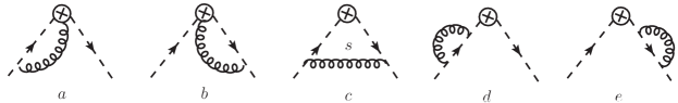
Figure 2: The next-to-leading SCET diagrams describing the contribution $\hat{\mathcal{F}}_{\text{NLO}}^{q}$ in SCET-I.

The vertex of the operator is shown by the crossed circle. The dashed lines denote the hard-collinear quarks, the gluon lines in diagrams $(a,b,d,e)$ are also hard-collinear. The soft gluon line in diagram $(c)$ is indicated by index $s$.

The QCD perturbative expansion on the lhs of Eq.(77) is given by the QCD diagrams describing the Compton scattering on a quark $\gamma q\rightarrow\gamma q$. The leading order contribution is given by the tree diagrams with massless quarks. Computing these diagrams and comparing with the rhs of Eq.(77) one obtains the expression for the leading-order coefficient functions

$$C_{2}^{\text{{\tiny LO}}}(s,t) =-C_{4}^{\text{{\tiny LO}}}(s,t)=\frac{s-u}{su}=-\frac{1}{s}\frac{1+\cos^{2}\theta/2}{\sin^{2}\theta/2},$$ (83)

$$C_{6}^{\text{{\tiny LO}}}(s,t) =\frac{t}{su}=\frac{1}{s}\frac{\cos^{2}\theta/2}{\sin^{2}\theta/2}.$$ (84)

In order to obtain the $C_{\text{\tiny NLO}}^{\mu\nu\sigma}$ in Eq.(78) one has to compute the one-loop corrections to the matrix elements in Eq.(77). The QCD one-loop diagrams for the $T$-product of the electromagnetic currents are shown in Fig.3.

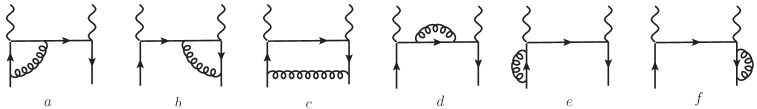
Figure 3: Next-to-leading order QCD diagrams required for the calculation of the $C^{\mu\nu\sigma}_{NLO}$. The crossed diagrams are not shown for simplicity.

As we already explained the leading order tree diagrams can be considered with the on-shell massless quarks. However beyond the tree level the situation is more complicated due to the IR- and UV-divergencies which must be regularized. The most convenient technique is to use the dimensional regularization (DR) with $D=4-2\varepsilon$ in order to treat all singularities which appear in the diagrams. We will use DR and the $\overline{\text{MS}}$-scheme in order to perform UV-renormalization of the matrix element $\langle O^{\sigma}\rangle$ on rhs of Eq.(77). The sum of the QCD diagrams in Fig.3 is UV-finite because of the non-renormalization theorem for the electromagnetic current. However UV-divergencies are presented in the individual vertex ($a,b$) and self-energy ($d,e,f$) diagrams in Fig.3 . We also use DR in order to evaluate corresponding UV-divergent integrals.

In order to treat IR-divergencies in the QCD diagrams in Fig.3 we consider the off-shell momenta for the outgoing quarks. The corresponding IR-singularities are logarithmic and therefore we consider the small off-shell momenta only in the denominators of the propagators and use the on-shell momenta in the numerators of the integrands. The nice feature of such approach is that UV-divergent integrals are IR-finite (because corresponding integrals are logarithmic) and they can be easily singled out. Therefore the IR-divergent contributions are UV-finite and can be computed in $D=4$ which allows one to easily perform the required manipulations with the Dirac algebra. Following this way we avoid a discussion about consistent representation of the matrix $\gamma_{5}$ in $D$ dimensions and possible mixing with the so-called evanescent operators. On the other hand such IR-regularization introduces more complicated integrals giving the IR-logarithms.

The sum of the QCD diagrams in Fig.3 can be interpreted as radiative corrections to the hard coefficient function and to the SCET-I matrix element

$$\sum_{i}D_{i}^{\mu\nu}=C_{\text{{\tiny NLO}}}^{\mu\nu\sigma}\ (s,t;\mu_{F}^{2})~{}\bar{u}_{n}\gamma^{\sigma}_{\perp}u_{\bar{n}}\ e^{2}_{q}\hat{\mathcal{F}}_{LO}^{q}+C_{\text{{\tiny LO}}}^{\mu\nu\sigma}(s,t)~{}\bar{u}_{n}\gamma^{\sigma}_{\perp}u_{\bar{n}}\ e^{2}_{q}\hat{\mathcal{F}}_{NLO}^{q}(t;\mu_{F}^{2},p^{2},p^{\prime 2}).$$ (85)

Here $D_{i}^{\mu\nu}$ denotes the contribution of each diagram in Fig.3 (up to the simple factor $\alpha_{s}/\pi$). In Eq.(85) we show explicitly the dependence on the factorization scale $\mu_{F}$ and on the IR-regulators $p^{2}$ and $p^{\prime 2}$. In order to obtain $C_{\text{{\tiny NLO}}}^{\mu\nu\sigma}$ we need to compute the following difference

$$C_{\text{{\tiny NLO}}}^{\mu\nu\sigma}(s,t;\mu_{F}^{2})\ e^{2}_{q}\bar{\xi}_{n}\gamma_{\bot}^{\sigma}\xi_{\bar{n}}=\sum_{i}D_{i}^{\mu\nu}-\bar{u}_{n}\gamma^{\sigma}_{\perp}u_{\bar{n}}\ C_{\text{{\tiny LO}}}^{\mu\nu\sigma}(s,t)\ e^{2}_{q}\hat{\mathcal{F}}_{NLO}^{q}(t;\mu_{F}^{2},p^{2},p^{\prime 2}).$$ (86)

The sum of the QCD diagrams $D_{i}^{\mu\nu}$ depends on the soft scales $p^{2}$ and $p^{\prime 2}$ but does not depend on the factorization scale $\mu_{F}$. However the soft scales must cancel on the rhs of Eq.(86). This cancellation provides a powerful check of the derived factorization theorem. It is clear that the dependence on the factorization scale of the $C_{\text{{\footnotesize NLO}}}^{\mu\nu\sigma}$ is related with the renormalization properties of the SCET-I operator $O^{\sigma}$. The renormalization of $O^{\sigma}$ was already studied in the literature. A more detailed discussion can be found, for instance, in Ref.[43]. This operator is multiplicatively renormalizable and using the independence of the physical amplitude from the factorization scale $\mu_{F}\equiv\mu$ one can derive the RG-equation for the coefficient function

$$\mu\frac{d}{d\mu}C^{\mu\nu\sigma}(s,t;\mu^{2})=\frac{\alpha_{s}}{4\pi}C_{F}\left\{\ 4\ln[-t/\mu^{2}]-6+\mathcal{O}(\alpha_{s})\right\}C^{\mu\nu\sigma}(s,t;\mu^{2}),$$ (87)

where as usually $C_{F}=(N^{2}_{c}-1)/2N_{c}$. The expression in the figured brackets on the rhs of Eq.(87) is the leading-order anomalous dimension of the operator $O^{\sigma}$ [43].

A detailed discussion of the calculation of the rhs in Eq.(86) is presented in the Appendix B. Here we provide only the main results for the scalar coefficient functions $C_{i}$ defined in Eq.(31). Let us define their perturbative expansion as

$$C_{i}(s,t;\mu^{2})=C_{i}^{\text{{\tiny LO}}}(s,t)+\frac{\alpha_{s}}{4\pi}C_{F}~{}C_{i}^{\text{{\tiny NLO}}}(s,t;\mu^{2})+\mathcal{O}(\alpha_{s}^{2}).$$ (88)

The leading-order coefficients $C_{i}^{\text{{\tiny LO}}}$ are presented in Eqs.(83)-(84). At the next-to-leading order we obtained the following expressions

$$C_{2}^{\text{{\tiny NLO}}}(s,t;\mu^{2}) =C_{2}^{\text{{\tiny LO}}}(s,t)\left\{-\ln^{2}[-t/{\mu}^{2}]+3\ln[-t/{\mu}^{2}]\right\}+\frac{t^{2}-su}{s^{2}u^{2}}\left(u\ln^{2}\left[\frac{u}{t}\right]-s\ln^{2}\left[\frac{s}{t}\right]\right)$$

$$-\left(\frac{3}{s}+\frac{2}{u}\right)\ln\left[\frac{s}{t}\right]+\left(\frac{3}{u}+\frac{2}{s}\right)\ln\left[\frac{u}{t}\right]-5\frac{s-u}{su}-\pi^{2}\frac{s-u}{su}\left(\frac{t^{2}}{su}-\frac{7}{6}\right),$$ (89)

$$C_{4}^{\text{\tiny NLO}}(s,t;\mu^{2}) =C_{4}^{\text{{\tiny LO}}}\left\{-\ln^{2}[-t/{\mu}^{2}]+3\ln[-t/{\mu}^{2}]\right\}-\frac{t^{2}-su}{s^{2}u^{2}}\left(u\ln^{2}\left[\frac{u}{t}\right]-s\ln^{2}\left[\frac{s}{t}\right]\right)$$

$$+\left(\frac{3}{s}+\frac{2}{u}\right)\ln\left[\frac{s}{t}\right]-\left(\frac{3}{u}+\frac{2}{s}\right)\ln\left[\frac{u}{t}\right]+9\frac{s-u}{su}+\pi^{2}\frac{s-u}{su}\left(\frac{t^{2}}{su}-\frac{7}{6}\right),$$ (90)

$$C_{6}^{\text{\tiny NLO}}(s,t;\mu^{2}) =C_{6}^{\text{{\tiny LO}}}\left\{-\ln^{2}[-t/{\mu}^{2}]+3\ln[-t/{\mu}^{2}]\right\}-\frac{t^{2}+su}{s^{2}u^{2}}\left(s\ln^{2}\left[\frac{s}{t}\right]+u\ln^{2}\left[\frac{u}{t}\right]\right)$$

$$-\left(\frac{3}{s}+\frac{2}{u}\right)\ln\left[\frac{s}{t}\right]-\left(\frac{3}{u}+\frac{2}{s}\right)\ln\left[\frac{u}{t}\right]-7\frac{t}{su}+\pi^{2}\frac{t}{su}\left(\frac{t^{2}}{su}+\frac{7}{6}\right).$$ (91)

One sees that the soft scales $p^{2}$ and $p^{\prime 2}$ are not present in Eqs.(89)-(91) because they cancel as it is required by the factorization. One can also easily check that the scale dependence in the obtained $C_{i}^{\text{\tiny NLO}}$ is in agreement with the RG-equation (87). The leading-order coefficients $C_{i}^{\text{\tiny LO}}$ are real but the next-to-leading expressions in Eqs.(89-91) have the nontrivial imaginary part which appears due to the logarithm $\ln[s/t]\equiv\ln[-s/|t|-i0]$. One can also observe that the expressions for the coefficients $C_{2,4}^{\text{\tiny NLO}}$ differ from their counterparts in the leading-order approximation not only by the relative sign, but also by the simple rational term

$$C_{2}^{\text{\tiny NLO}}+C_{4}^{\text{\tiny NLO}}=4\frac{s-u}{su}.$$ (92)

4 Phenomenology

In order to apply the factorization formula Eq.(31) in a phenomenological analysis one must define the unknown nonperturbative form factor $\mathcal{F}_{1}$. But there is one more difficulty hidden in the factorization expression (31). This problem is related to the careful separation of the soft and collinear region and in developing a technique for a systematic resummation of the large rapidity logarithms. Let us recall that the FF $\mathcal{F}_{1}$ implicitly depends on the specific rapidity regularization which helps to separate the soft and collinear regions. At present such a full description still remains a challenge. Meanwhile a useful phenomenological consideration can be carried out. This is possible due to the universality of the definition of the SCET FF $\mathcal{F}_{1}$ in the factorization approach and due to its specific properties. This one unknown quantity describes the three independent amplitudes $T_{2,4,6}$. Therefore the idea is to re-express this quantity in terms of any one amplitude and then use this expression for the remaining two amplitudes. This allows one to establish the relation between the three amplitudes up to well defined hard-spectator corrections.

In order to be specific let us use Eq.(31) and write for $\mathcal{F}_{1}$ the following expression

$$\mathcal{F}_{1}(t)=\mathcal{R}(s,t)-\mathbf{\Psi}\ast H_{2}(s,t)\ast\mathbf{\Psi}/C_{2}(s,t).$$ (93)

Here we define the ratio

$$\mathcal{R}(s,t)=\frac{T_{2}(s,t)}{C_{2}(s,t,{\mu}^{2}=-t)}.$$ (94)

Note that the rhs of Eq.(93) does not depend on the total energy $s$. Substituting this equation in the expressions for the amplitudes $T_{4,6}$ (31) we obtain

$$T_{i}(s^{\prime},t)=C_{i}(s^{\prime},t)\mathcal{R}(s,t)+\mathbf{\Psi}\ast\left\{H_{i}(s^{\prime},t)-C_{i}(s^{\prime},t)\frac{H_{2}(s,t)}{C_{2}(s,t)}\right\}\ast\ \mathbf{\Psi.}$$ (95)

On the left side of this equation we have a well defined physical amplitude therefore the right side must also be well defined. This means that the potential end-point singularities in the hard-spectator corrections must cancel in the difference on the rhs of Eq.(95). We assume that all the hard coefficient functions in Eq.(95) are defined at ${\mu}^{2}=-t$. We also used the different values of the total energy $s^{\prime}$ in Eq.(95) in order to stress that the substitution (93) does not depend on the energy $s$.

If the values of the hard-spectator contributions in Eq.(95) are small, then such terms can be neglected and we obtain

$$T_{i}(s^{\prime},t)\simeq C_{i}(s^{\prime},t)\mathcal{R}(s,t)\Leftrightarrow\frac{T_{i}(s^{\prime},t)}{C_{i}(s^{\prime},t)}\simeq\mathcal{R}(s,t).$$ (96)

Notice that this formula is valid to all orders in $\alpha_{s}$ for the coefficient $C_{i}$ but at order $\alpha_{s}^{2}$ one has to take into account the hard-spectator corrections.

Obviously the choice of the amplitude $T_{i}$ for the definition of the ratio $\mathcal{R}$ in (94) does not play any essential role. In the definition (94) we also used a freedom to fix the factorization scale and chose $\mu^{2}=-t$ as simplest realization.

If the bulk contribution to the amplitudes $T_{i}(s,t)$ is provided by the soft-overlap term then one expects that the ratio $\mathcal{R}$ depends only very weakly on the energy $s$

$$\frac{d}{ds}\mathcal{R}(s,t)\simeq\mathcal{O}(\alpha_{s}^{2}),$$ (97)

where the higher order corrections $\sim\mathcal{O}(\alpha_{s}^{2})$ are again given by the hard-spectator contributions and assumed to be relatively small. This picture can be verified when comparing with the data.

Consider the formula (15) for the cross section. Using expressions (96) for the amplitudes $T_{2,4,6}$ and neglecting the helicity flip amplitudes $T_{1,3,5}\simeq 0$ and power suppressed terms $\sim m/Q$ we obtain

$$\ \frac{d\sigma}{dt}=\frac{\pi\alpha^{2}}{s^{2}}~{}|\mathcal{R}(s,t)|^{2}(-su)\left(\frac{1}{2}|C_{2}(s,t)|^{2}+\frac{1}{2}|C_{4}(s,t)|^{2}+|C_{6}(s,t)|^{2}\right).$$ (98)

If the ratio $\mathcal{R}(s,t)$ depends mostly on the momentum transfer $t$ then the energy dependence of the cross section in Eq.(98) is defined only by the hard coefficient functions. To the leading-order accuracy using Eqs.(83),(84) one obtains

$$\ \frac{d\sigma}{dt}\simeq\left.\frac{2\pi\alpha^{2}}{s^{2}}~{}|\mathcal{R}(s,t)|^{2}\left(\frac{s}{-u}+\frac{-u}{s}\right)\right|_{m=0}=\frac{d\sigma_{0}^{\text{KN}}}{dt}|\mathcal{R}(s,t)|^{2}.$$ (99)

Here only the the ratio $\mathcal{R}$ provides the difference from the point-like Klein-Nishina cross section $d\sigma_{0}^{\text{KN}}$ due to the nucleon structure. This simple leading-order formula is modified by the corrections from the QCD hard subprocess. To the next-to-leading accuracy one finds

$$\ \frac{d\sigma}{dt}\simeq\frac{d\sigma_{0}^{\text{KN}}}{dt}|\mathcal{R}(s,t)|^{2}\left(1+\frac{\alpha_{s}}{4\pi}C_{F}\frac{C_{2}^{\text{\tiny LO}}\text{Re}\left[C_{2}^{\text{\tiny NLO}}-C_{4}^{\text{\tiny NLO}}\right]+C_{6}^{\text{\tiny LO}}\text{Re}\left[C_{6}^{\text{\tiny NLO}}\right]}{|C_{2}^{\text{\tiny LO}}|^{2}+|C_{6}^{\text{\tiny LO}}|^{2}}\right),$$ (100)

where we used that the leading order coefficient functions are real and $\left|C_{2}^{\text{\tiny LO}}\right|=\left|C_{4}^{\text{\tiny LO}}\right|$.

This result allows one to extract the absolute value $|R(s,t)|$ and check the equation Eq.(97) using the experimental data for the cross section. Using Eq.(100) one easily obtains

$$|\mathcal{R}(s,t)|\approx\sqrt{\frac{d\sigma^{\text{exp}}/dt}{d\sigma_{0}^{\text{KN}}/dt}}\left(1-\frac{1}{2}\frac{\alpha_{s}}{4\pi}C_{F}\frac{C_{2}^{\text{\tiny LO}}\text{Re}\left[C_{2}^{\text{\tiny NLO}}-C_{4}^{\text{\tiny NLO}}\right]+C_{6}^{\text{\tiny LO}}\text{Re}\left[C_{6}^{\text{\tiny NLO}}\right]}{|C_{2}^{\text{\tiny LO}}|^{2}+|C_{6}^{\text{\tiny LO}}|^{2}}\right).$$ (101)

In obtaining this formula we neglected by the all power corrections suppressed as $\mathcal{O}(1/Q)$. Nevertheless the mass of the nucleon is not too small as compared to the values of the energy $s$ and momentum transfer $-t$ and therefore the power corrections may still provide a sizeble numerical effect. In order to estimate their size we suggest to include in our considerations at least the so-called kinematical power corrections. We define them in the following way. We again neglect the helicity flip amplitudes $T_{1,3,5}\simeq 0$ but use the exact kinematical coefficients with the nucleon mass $m$ in Eq.(15). In this case we obtain

$$\frac{d\sigma}{dt} = \frac{\pi\alpha^{2}}{(s-m^{2})^{2}}|\mathcal{R}|^{2}\left\{(s-m^{2})(m^{2}-u)\frac{1}{2}(|\bar{C}_{2}|^{2}+|\bar{C}_{4}|^{2})+(m^{4}-su)|\bar{C}_{6}|^{2}\right\}.$$ (102)

The coefficient functions $\bar{C}_{i}$ in the expression (102) are the functions of $s$ and $t$ which are defined in the exact kinematics with $m\neq 0$ and therefore they include the powers of $m/s$. We define these functions from the massless expressions $C_{i}(s,\cos\theta)$ computed above in the following way:

$$\bar{C}_{i}(s,t)=C_{i}\left(s,\cos\theta=1+\frac{2ts}{(s-m^{2})^{2}}\right)=\left.C_{i}(s,\cos\theta)\right|_{m=0}+\mathcal{O}(m/s).$$ (103)

In other words, in the massless kinematics in the expressions for $\left.C_{i}(s,\theta)\right|_{m=0}$ we identify the massless variables with the exact energy $s$ and scattering angle $\theta$ substituting $\cos\theta=1+\frac{2ts}{(s-m^{2})^{2}}$. In what follow we denote the absolute value $|\mathcal{R}|$ which is obtained using Eq.(102) as $|\bar{\mathcal{R}}|$

$$|\bar{\mathcal{R}}|=\sqrt{\frac{d\sigma^{\text{exp}}}{dt}}:\sqrt{\frac{\pi\alpha^{2}}{(s-m^{2})^{2}}\left((s-m^{2})(m^{2}-u)\frac{1}{2}(|\bar{C}_{2}|^{2}+|\bar{C}_{4}|^{2})+(m^{4}-su)|\bar{C}_{6}|^{2}\right)}.$$ (104)

In the numerical calculations we expanded the rhs of Eq.(104) with respect to $\alpha_{s}$.

The data points for the cross section $d\sigma^{\text{exp}}$ at large $s$, $-t$ and $-u$ were published in Ref.[11]. In our analysis we use only the data for which $|u|,|t|\geq 2.5$ GeV². In computing the next-to-leading contribution we use the running coupling $\alpha_{s}(\mu^{2}=1.5$ GeV${}^{2})=0.360$ with $n_{f}=4$ and define the scale for the running coupling as $\mu^{2}=\min\{-t,-u\}$.

Our numerical results for the $|\mathcal{R}|$ and $|\bar{\mathcal{R}}|$ are shown in Fig.4 and Fig.5, respectively.

Figure 4: The extracted values of $|\mathcal{R}|$ as a functions of the momentum transfer in the leading-order (open squares) and next-to-leading order (color circles) approximations for the hard coefficient functions $C_{i}$ . The solid line demonstrates the fit of the NLO $|\mathcal{R}|$ using the power behavior as in Eq.(105). The shaded area shows the $99\%$ confidence bands.

The absolute value of the NLO corrections do not exceed $6\%$ in the accessible interval of $-t=2.5-6.5$ GeV². For the small values of the momentum transfer the RCs are negative but they change the sign around $-t=3.5-4$ GeV² and became positive. The largest effect from the radiative corrections is observed for the boundary values $-t=2.5$ GeV² and $-t=6.46$ GeV². In this case the NLO contributions for massless case reduce the value of $|\mathcal{R}|$ by $5\%$ for $s=10.9$ GeV². This leads to a bit larger sensitivity of the $|\mathcal{R}|_{NLO}$ to the variable $s$ at $t=-2.5$ GeV² comparing to $|\mathcal{R}|_{LO}$. The effect from the RCs for the $\bar{\mathcal{R}}$ is quite similar. Taking into account that the hard-spectator contribution provides of about $10\%$ of the cross section [7, 8, 9, 10] we can conclude that computed NLO corrections provide a comparable numerical effect.

The inclusion of the power corrections as described above reduce the absolute value of $\bar{\mathcal{R}}$ in the interval $0-13\%$ for the different values of $-t$. One can also observe that the extracted values $\bar{\mathcal{R}}$ are less sensitive to the value of $s$ than ${\mathcal{R}}$. This may indicate that the more sensitive to $s$ behavior of ${\mathcal{R}}$ can be associated with the power corrections.

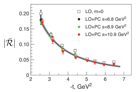
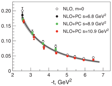
Figure 5: The extracted values of $|\bar{\mathcal{R}}|$ as a function of the momentum transfer obtained using the leading-order (left plot) and next-to-leading (right plot) order approximations for the hard coefficient functions $\bar{C_{i}}$. The open squares (rhombs) show the LO (NLO) values extracted with $m=0$ using Eq.(101). The solid lines show the fit of the $|\bar{\mathcal{R}}|$ with the formula in Eq.(105). The shaded area shows the $99\%$ confidence bands.

In the figures describing the ratio ${\mathcal{R}}$ we show the empirical fit of the extracted points (solid line) together with the 99% confidence bands (gray shaded area). For the empirical fit we used a simple power function

$$|\mathcal{R}(s,t)|=\left(\frac{\Lambda^{2}}{-t}\right)^{\alpha}.$$ (105)

where $\alpha$ and $\Lambda$ are unknown fitting parameters. The results of the fit for different cases are shown in Table 1. One can see there that $\chi^{2}$/d.o.f is much better for $\bar{\mathcal{R}}$ extracted with the kinematical power corrections. This is the consequence of the less sensitive behavior of the extracted points for $\bar{\mathcal{R}}$ with respect to energy $s$ as we discussed above.

Table 1: Results for the parameters $\Lambda$ and $\alpha$ defining the behavior (105) for the ratios $|\mathcal{R}|$ in Fig.4 and $|\bar{\mathcal{R}}|$ in Fig.5

	$\Lambda$, GeV	$\alpha$	$\chi^{2}$/d.o.f
$|\mathcal{R}|$, NLO	$0.95\pm 0.02$	$1.67\pm 0.05$	$2.7$
$|\bar{\mathcal{R}}|$, LO	$1.0\pm 0.02$	$1.88\pm 0.05$	$1.1$
$|\bar{\mathcal{R}}|$, NLO	$0.98\pm 0.02$	$1.80\pm 0.05$	$1.25$

It is also interesting to note that obtained results for the exponent $\alpha$ are somewhat smaller than the expected asymptotic power behavior obtained from the SCET analysis: $|\mathcal{R}(s,t)|\sim{(-t)}^{-2}$. But for the discussed values of the momentum transfer $-t\simeq 2.5-7$GeV² the hard-collinear scale $\mu_{hc}\simeq\sqrt{\Lambda Q}$ is still quite small. Therefore we expect that these empirical values of $\alpha$ can be a result of the oversimplified choice of the fit formula in Eq.(105). The measurements of the cross section for the higher values of $-t$ can help to clarify this situation. In Fig.6 we show the ratio $\bar{\mathcal{R}}$ as a function of energy $s$ at fixed values of $t$ and compare with the obtained fit.

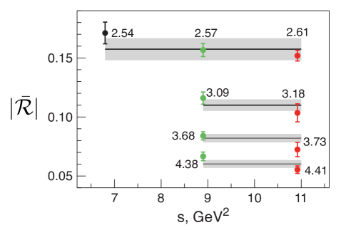
Figure 6: The ratio $\bar{\mathcal{R}}$ as a function of energy $s$ at fixed values of $t$. The fit and bounds are the same as on the right plot in Fig.5.

The other measured observables which are very helpful in order to clarify the underlying partonic dynamics are given by the recoil polarizations $K_{\text{LL}}$ and $K_{\text{LS}}$. They can be constructed for the circular polarized photon ($R,L$) and longitudinal ($\|$) or transverse ($\bot$) polarization of the recoiling proton. In the current work we consider only the longitudinal polarization $K_{\text{LL}}$ because it does not depend on the helicity flip amplitudes in the leading power approximation. Its definition reads

$$K_{\text{LL}}=\frac{\sigma_{\|}^{R}-\sigma_{\|}^{L}}{\sigma_{\|}^{R}+\sigma_{\|}^{L}}.$$ (106)

Computing this asymmetry with the help of the approximation Eq.(96) we obtain that the unknown factor $|R|$ cancels in the ratio and the asymmetry is defined only by the perturbative coefficients $C_{i}$.

Neglecting all power corrections and using the next-to-leading expressions we obtain

$$K_{\text{LL}} =\frac{s^{2}-u^{2}}{s^{2}+u^{2}}-\frac{\alpha_{s}}{\pi}C_{F}\frac{1}{\left(s^{2}+u^{2}\right)^{2}}\left\{~{}(t-s)u^{3}\ln^{2}\left[|u|/|t|\right]-(t-u)s^{3}\ln^{2}\left[s/|t|\right]\right.$$

$$\left.+su^{2}(2t-s)\ln\left[|u|/|t|\right]-us^{2}(2t-u)\ln\left[s/|t|\right]-\pi^{2}(s-t)u^{3}~{}\right\}+\mathcal{O}(\alpha_{s}^{2}),$$ (107)

The leading-order contribution in this expression reproduces the well-known expression for the Klein-Nishina asymmetry which describes the scattering on the point-like massless particles. Obviously, this term does not depend on energy $s$ if we rewrite $u$ in terms of $s$ and scattering angle $\theta$ in the massless approximation. The weak logarithmic $s$-dependence is introduced by the QCD radiative correction through the definition of the scale for the running coupling $\alpha_{s}$.

In Fig.7 (left plot) we show the numerical results for the asymmetry $K_{\text{LL}}$ as a functions of the scattering angle $\theta$. The solid red line corresponds to the leading-order approximation in Eq.(107) (massless Klein-Nishina asymmetry). The dashed (blue) and dotted (black) lines show the numerical results for the complete NLO expression (107) for the energies $s=6.9$ GeV² and $s=20$ GeV², respectively. The data point corresponds to $s=6.9$ GeV² [12]. We see that the energy dependence of the NLO expression remains quite weak. The estimates which are obtained are larger than the experimental data point. However for this energy and angle $\theta=121.6^{o}$ the value of the $-u=1.14$ GeV² is still quite small. For clarity we show with the help of the solid thick (blue) line the values of $K_{\text{LL}}$ in the kinematical interval where $-t\geq 2.5$ GeV² and $-u\geq 2.5$ GeV² for $s=6.9$ GeV². Keeping in mind the estimates of the cross section one can expect that the power corrections for this kinematical region can still provide a sizeble numerical effect.

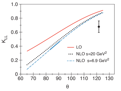
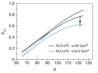
Figure 7: The longitudinal asymmetry $K_{\text{LL}}$ as a function of scattering angle $\theta$. Left plot: comparison of the LO (red solid) and NLO results computed with $s=6.9,20$ GeV², (dashed and dotted lines, respectively). The kinematical power corrections (PC) are neglected $m=0$. Right plot: comparison of the NLO results computed with (solid black and blue lines) and without kinematical power corrections. The curves for the massless approximation are the same as on the left plot.

Therefore in order to estimate the possible effect from the power suppressed contributions we include into consideration the kinematical power corrections in the same way as we did for the cross section before. The numerical results are presented in Fig.7 (right plot). One can observe that the computed power corrections provide a sizeble effect for large angles ($\theta>90^{o}$) and quite small for the $\theta\leq 90^{o}$. We see that their effect for energy $s=6.9$ GeV² is quite large and negative bringing the curve in agreement with the data point. One can also observe that their effect for large energy $s=20$ GeV² and large angle $\theta=120^{o}$ ($-u=4.5$ GeV²) is approximately a factor of three smaller but is still quite sizeble numerically.

5 Discussion

We provided a detailed consideration of the QCD factorization for the WACS process. Using the SCET framework we proved that the leading-power or dominant contribution is described by the soft- and hard-spectator scattering. For asymptotically large values of the Mandelstam variables the soft-spectator contribution is strongly suppressed by the Sudakov logarithms but not by powers of a generic large scale $Q$. In the region of moderate values of $Q^{2}$ where the hard-collinear scale $\mu_{hc}\sim\sqrt{Q\Lambda}$ is still quite small this logarithmic suppression is weak and therefore one must include the soft-spectator contribution on the same footing as the hard one. We provided the factorization formulas for the three amplitudes describing the scattering when the nucleon helicity is conserved. The amplitudes corresponding to the helicity flip scattering are suppressed as $1/Q$ relative to the helicity conserving ones. In the present work, we did not include these subleading amplitudes in the current analysis.

In the SCET framework the soft-spectator contribution is described only by one SCET-I form factor $\mathcal{F}_{1}$ which must be considered as a non-perturbative function in the region of moderate values of $Q^{2}$. This form factor depends only on the momentum transfer $t$ due to the underlying hard-collinear scattering. This feature allows one to define the $s$-behavior of the amplitudes computing the hard coefficient functions. The tree level hard coefficient functions to the soft-spectator part have been computed in Ref.[36]. Here we also presented the next-to-leading QCD corrections to these quantities. This calculation provide a direct check of the factorization for the soft-spectator part beyond the tree approximation.

Unfortunately the SCET-I form factor $\mathcal{F}_{1}$ is sensitive to the overlap between the soft and collinear regions. This can be seen explicitly when one performs the factorization of the hard-collinear modes. The same feature also leads to the end-point singularities in the hard-spectator contribution, see e.g. [35]. Hence one has to imply a certain rapidity regularization in order to unambiguously define the soft- and hard-spectator contributions. Then the form factor $\mathcal{F}_{1}$ and the hard-spectator contribution also depend on the factorization scale associated with the rapidity regularization. In order to avoid this difficulty we used the physical subtraction scheme and excluded the form factor $\mathcal{F}_{1}$ rewriting it in terms of one physical amplitude. This allows us to obtain the well defined relations Eq.(95) between all three dominant amplitudes. The unknown nonperturbative dynamics describing the soft-overlap configuration is included in the ratio $\mathcal{R}(s,t)$ defined in Eq.(94). This quantity can be extracted from the analysis of existing data.

In the phenomenological analysis these relations can be further simplified if the hard-spectator contribution is quite small in the region of moderate values of $Q^{2}$ and therefore can be neglected. Such an assumption looks to be reliable because the hard-spectator coefficient functions are suppressed as $\mathcal{O}(\alpha^{2}_{s})$. In addition, the existing calculations demonstrate that the hard-spectator mechanism predicts cross section which are one order of magnitude smaller than the experimental data [7, 8, 9, 10].

The dominance of the soft-spectator configuration can be checked through the $s$-dependence of the ratio $\mathcal{R}(s,t)$. If the contribution of the hard-spectator mechanism is relatively small then the bulk of this dependence is described by the hard-coefficient function in the soft-spectator term and must cancel according to Eq.(94). We extracted the value of the ratio $\mathcal{R}(s,t)$ using the existing data for different values of $s$ and $t$. We performed the leading order and the next-to-leading order analysis and also investigated the effect of the kinematical power corrections. The main qualitative conclusion is that for the region where $|t|,|u|\geq 2.5$ GeV² a weak $s$-dependence is observed. In Fig.4 one can see that the data for the same $t$ and different $s$ differ by $15-20\%$. However, the existing data cover the region of relatively small values of $s$ and $t$. They can however still be affected from power corrections. In order to estimate their effect we included the kinematical power corrections which describe the simple powers of $m/Q$ arising from the exact hadronic kinematics in the expression for the cross section. In this case the ratio $\mathcal{R}(s,t)$ is less sensitive to the energy $s$ as one can see in Fig.5. The difference between the extracted values of $\mathcal{R}(s_{i},t)$ are around $11-13\%$. These results allow us to conclude that existing data are in a good agreement with the assumption about the dominance of the soft-spectator contribution.

Further measurements of the cross section for higher values of the Mandelstam variables can be very helpful in order to continue to study and to constrain the ratio $\mathcal{R}(s,t)$. The higher values $s$, $t$ and $u$ will allow one to reduce the effect of the power corrections and to investigate much better the role of the different logarithmic QCD corrections. We suppose that the hard-spectator corrections which can provide the effect of order $10\%$ must also be included in the phenomenological analysis.

The factorization framework allows one to use the extracted ratio $\mathcal{R}$ for the analysis of the other processes. In Ref.[36] it was shown that this function also describes the soft-spectator contribution in the two-photon exchange (TPE) correction in the elastic lepton proton scattering. The future experiments will allow to measure the elastic cross section up to $Q^{2}=17$ GeV². Therefore in order to reduce the ambiguity in the extraction of the electromagnetic form factors one need to reduce the ambiguity from TPE correction. Therefore we suppose that the WACS provide us the best possibility to obtain the required information about this nonperturbative function.

The different WACS asymmetries can also provide an effective way to study the detailed underlying hadron dynamics. We demonstrated that in case of the dominance of the soft-spectator contribution the longitudinal polarization $K_{\text{LL}}$ can be computed in terms of the hard coefficient functions. Unfortunately the existing data point corresponds to a very low value of $-u=1.14$ GeV². The inclusion of the kinematical power corrections allows us to describe the asymmetry $K_{\text{LL}}$, although the present treatment of power corrections is mainly meant to indicate the sensitivity of the present data to such effects. We think that new data for $K_{\text{LL}}$ at higher values of energy and momentum transfer will be very useful in order to clarify unambiguously the role of the soft-overlap mechanism. From the theoretical side it is also important to clarify the contribution of the helicity flip amplitudes which are required in order to describe the transverse polarization $K_{\text{LS}}$ and in order to reduce the corresponding ambiguity in other observables.

Appendix A

Here we discuss the soft-overlap contributions involving the photon states. The set of the corresponding operators must consist at least from the three different collinear fields associated with the light-cone vectors $n,\bar{n}$ (nucleon sectors) and $v,\bar{v}$ (photon sectors). Therefore the simplest set of the operators reads

$$\tilde{O}^{(3)}=\left\{\bar{\chi}_{v}\mathcal{A}_{\bot}^{\bar{n}}\chi_{n},~{}...\right\},$$ (108)

where dots describe the analogous operators but with the different hard-collinear fields. The factorization of the amplitude in this case can be described by the diagrams in Fig.8.

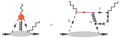
Figure 8: The diagrams describing the configuration with the three-particle soft-overlap described by the SCET operator in Eq.(109). The hard blob is shown by red color. The indices near the hard-collinear lines show the collinear sector. The soft quarks are shown by solid lines with the crosses.

This configuration describes the soft-overlap between the nucleons and outgoing photon state. One soft quark is attached to the photon vertex. For simplicity, the soft-overlap part associated with the nucleon sector is shown by the gray blob. In this case the hard-collinear dynamics is described by the following SCET matrix element

$$\left\langle p^{\prime},q^{\prime}\right|\tilde{O}_{1}^{(3)}\left|p\right\rangle_{\text{\tiny SCET}}.$$ (109)

We need to compare the contribution of this matrix element to the contribution of the matrix element in Eq.(37). In order to perform this comparison we proceed in the following way

$$\left\langle p^{\prime},q^{\prime}\right|\tilde{O}_{1}^{(3)}\left|p\right\rangle_{\text{\tiny SCET}}=\left\langle p^{\prime},q^{\prime}\right|T\{\tilde{O}_{1}^{(3)},\mathcal{L}_{\text{int}}^{(2,v)}[\bar{q}B^{c}_{\bot}\xi],\mathcal{L}_{\text{int}}^{(1,n)}[\bar{\xi}A_{\bot}q]\}\left|p\right\rangle_{\text{\tiny SCET}}$$ (110)

$$=iee_{q}\varepsilon^{*}_{\mu}\left\langle p^{\prime}\right|\int d^{4}x\ e^{i(q^{\prime}x)}T\{\tilde{O}_{1}^{(3)},\ \bar{q}(x_{-})\gamma^{\mu}\xi_{v}(x),\mathcal{L}_{\text{int}}^{(1,n)}[\bar{\xi}A_{\bot}q]\}\left|p\right\rangle_{\text{\tiny SCET}}.$$ (111)

Here the interaction vertex $\mathcal{L}^{(2,v)}_{\text{int}}[\dots]$ describes the interaction of the collinear photon (field $B^{c}_{\bot}$) with hard-collinear and soft quarks. The interaction $\mathcal{L}_{\text{int}}^{(1,n)}[\dots]$ is given in Eq.(53). Computing the contractions in Eq.(111) one obtains the diagram shown on the rhs in Fig.8. In order to perform the complete matching to SCET-II one must add additional vertices in Eq.(111) which are required for description of the hard-collinear interactions associated with the $n$ and $\bar{n}$ collinear sectors. These insertions can be constructed in the same way as in $T$-product in Eq.(74) in the each collinear sector. After that one obtains the following result, (using the same notations as in Eq.(45):

$$\int d^{4}x\ e^{i(q^{\prime}x)}T\{\tilde{O}_{1}^{(3)},\ \bar{q}(x_{-})\gamma^{\mu}\xi_{v}(x),\dots\}\simeq J_{v}^{\gamma}\ast O_{n}^{(6)}\ast J_{n}\ast\tilde{O}_{S}\ast J_{\bar{n}}\ast O_{\bar{n}}^{(6)},$$ (112)

where the jet -function $J_{v}^{\gamma}$ describes the hard-collinear fluctuations associated with the outgoing photon.

The relative order of the matrix elements (37) and (109) can be obtained from the estimate of the operator in the matrix element (111). For that operator one obtains

$$\int d^{4}x\ e^{i(q^{\prime}x)}T\{\tilde{O}_{1}^{(3)},\ \bar{q}(x_{-})\gamma^{\mu}\xi_{v}(x),\mathcal{L}_{\text{int}}^{(1,n)}[\bar{\xi}A_{\bot}q]\}\sim\mathcal{O}(\lambda^{4}).$$ (113)

Hence we can conclude that the contribution (109) is suppressed as $\mathcal{O}(\lambda^{2})$ compared to Eq.(37) and therefore can be neglected.

The one more possibility is provided by the soft-overlap of the all external states. In this case the factorization of the hard modes provides the four-quark operator (for simplicity we do not show the indices of the fields):

$$\tilde{O}^{(4)}=\bar{\chi}_{n}\chi_{\bar{n}}~{}\bar{\chi}_{\bar{v}}\chi_{v}~{}.$$ (114)

Such operator arises from the diagram with the hard gluon exchange as shown in Fig.9.

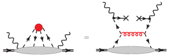
Figure 9: An example of the diagram desribing the soft-overlap contribution with the operator $\tilde{O}^{(4)}$ Eq.(114). For simplicity the gray blob on rhs denotes the hard-collinear and soft particles which describe the collinear sectors associated with the nucleon states. The red gluon line denotes the hard gluon exchange. The interactions of the photons with quarks are described by the SCET vertices $\mathcal{L}_{\text{int}}^{(2,v)}[\bar{\xi}B^{c}_{\bot}q]$ and $\mathcal{L}_{\text{int}}^{(2,\bar{v})}[\dots]$ with the collinear photon fields.

In order to compare this contribution with the soft-overlap described by FF $\mathcal{F}_{1}$ we have to compare the matrix elements (37) with

$$\left\langle p^{\prime},q^{\prime}\right|\tilde{O}^{(4)}\left|p,q\right\rangle_{\text{\tiny SCET}}=-e^{2}e^{2}_{q}\varepsilon_{\nu}\varepsilon^{*}_{\mu}$$

$$\phantom{-e^{2}e^{2}_{q}\varepsilon_{\nu}\varepsilon^{*}_{\mu}}\times\left\langle p^{\prime}\right|\int d^{4}x\int d^{4}y\ e^{i(q^{\prime}x)-i(qy)}T\{\tilde{O}^{(4)},\ \bar{\xi}_{v}(x)\gamma^{\mu}q,\bar{q}\gamma^{\nu}\xi_{\bar{v}}(y)\}\left|p\right\rangle_{\text{\tiny SCET}},$$ (115)

where we again do not show the interactions associated with the nucleon states. The calculation of the $T$-product in Eq.(115) can be illustrated by the diagram on rhs in Fig.9. The complete matching of the operator (9) onto SCET-II can be represented as

$$\int d^{4}x\int d^{4}y\ e^{i(q^{\prime}x)-i(qy)}T\left\{\bar{\chi}_{n}\chi_{\bar{n}}~{}\bar{\chi}_{\bar{v}}\chi_{v},\mathcal{L}_{\text{int}}^{(2,v)}[\bar{\xi}B^{c}_{\bot}q],\mathcal{L}_{\text{int}}^{(2,\bar{v})}[\bar{q}B^{c}_{\bot}\xi],...\right\}$$

$$\phantom{emptyspace}\simeq\left(J_{v}^{\gamma}\ast J_{\bar{v}}^{\gamma}\right)\ast O_{n}^{(6)}\ast J_{n}\ast\tilde{O}_{S}\ast J_{\bar{n}}\ast O_{\bar{n}}^{(6)},$$ (116)

where dots denote the insertions from the hard-collinear sectors associated with the nucleon states. Taking into account that

$$\int d^{4}x\int d^{4}y\ e^{i(q^{\prime}x)-i(qy)}T\{\tilde{O}^{(4)},\ \bar{\xi}_{v}(x)\gamma^{\mu}q(x),\bar{q}(y)\gamma^{\nu}\xi_{\bar{v}}(y)\}\sim\mathcal{O}(\lambda^{4}),$$ (117)

we can conclude that the matrix element in Eq.(115) is suppressed as $\mathcal{O}(\lambda^{2})$ comparing to the matrix element (37).

One more possibility is obtained when one of the photons is considered as a nonperturbative particle, like a hadron. The corresponding situation is described by the operator constructed from the hard-collinear and collinear fields, for instance

$$O^{(6)}_{\gamma}=\bar{\chi}_{n}\chi_{\bar{n}}~{}\bar{\chi}_{\nu}^{c}\chi_{\nu}^{c},$$ (118)

where we do not show the indices and the Dirac structures for simplicity. This operator arises after factorization of the hard modes in the diagram shown in Fig.10.

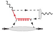
Figure 10: The diagram describing the factorization to the four-quark operator $O_{\gamma}$ defined in Eq.(118).

The collinear fields $\bar{\chi}_{\nu}^{c}\chi_{\nu}^{c}$ describe the nonperturbative overlap of the quarks with the external photon state. The corresponding matrix element is known as a photon distribution amplitude [41, 42]. However one can easily see that the photon matrix element introduces extra suppression factor $\lambda^{2}$

$$~{}\left\langle p^{\prime},q^{\prime}\right|\bar{\chi}_{n}\chi_{\bar{n}}~{}\bar{\chi}_{\nu}^{c}\chi_{\nu}^{c}\left|p\right\rangle_{\text{\tiny SCET}}\simeq\left\langle p^{\prime}\right|\bar{\chi}_{n}\chi_{\bar{n}}\left|p\right\rangle_{\text{\tiny SCET}}\left\langle q^{\prime}\right|\bar{\chi}_{\nu}^{c}\chi_{\nu}^{c}\left|0\right\rangle_{\text{\tiny SCET}}\sim\lambda^{2}\left\langle p^{\prime}\right|\bar{\chi}_{n}\chi_{\bar{n}}\left|p\right\rangle_{\text{\tiny SCET}}\text{.}$$ (119)

Hence this configuration is also subleading.

Appendix B

In this section we provide a detailed discussion of the calculation of the rhs of Eq.(86). The off-shell prescription which is used for the regularizations of IR-divergencies introduces the soft scale explicitly and this feature complicates the computation of the integrals for the matrix elements. One can simplify the straightforward calculation of required integrals using that only the difference on the rhs in Eq.(86) is needed. It is clear that if the factorization theorem is valid then the soft scales must cancel in the difference. One can observe this cancellation already at the level of the regularized integrals using the technique known as expansion by regions, see e.g. Refs.[44, 45].

In this approach the required integrals can be represented as a sum of the contributions associated with the hard, collinear and soft regions. The hard integrals does not depend on the soft scales because we need only the leading power contribution. Hence only the collinear and soft contributions can depend on the soft scales $p^{2}$ and $p^{\prime 2}$. The contribution from the soft region arises only in the box diagram $D^{\mu\nu}_{c}$ in Fig.3 and in the crossed box $\bar{D}^{\mu\nu}_{c}$. The contributions from the collinear regions are provided by the box diagram $D^{\mu\nu}_{c}$, vertex diagrams $D^{\mu\nu}_{a,b}$ and the crossed analogs $\bar{D}^{\mu\nu}_{a,b,c}$. The self-energy contributions $D^{\mu\nu}_{d},\bar{D}^{\mu\nu}_{d}$ have UV-divergencies and can be easily computed within the standard technique. Computing the quark wave function renormalizations we always apply the on-shell subtractions. We verified that on the rhs of Eq.(86) the soft contribution from the box diagram cancel with appropriate contribution from the unrenormalized diagram $(c)$ in Fig.2. Similarly, the collinear contributions associated with the quark momenta $p$ and $p^{\prime}$ cancel with the unrenormalized contributions provided by the diagrams $(a,b)$ in Fig.2.

In order to be specific let us present the contribution of the each QCD diagrams in Fig.3 as the following expression

$$\frac{\alpha_{s}}{\pi}D_{i}^{\mu\nu}=\bar{u}_{n}\gamma_{\bot}^{\sigma}u_{\bar{n}}\ e_{q}^{2}\frac{\alpha_{s}}{\pi}\sum_{k}N_{k}^{\mu\nu\sigma}(p,p^{\prime},q)J_{k}.$$ (120)

We imply that the expressions for each diagram $D^{\mu\nu}_{i}$ can be reduced to a set of the scalar integrals $J_{k}$ with the coefficients $N_{k}^{\mu\nu\sigma}(p,p^{\prime},q)$ depending only from the external momenta. This reduction is carried out in $D=4$ for the UV-finite expressions. The UV-divergent integrals in the vertex diagrams and the self-energy correction $D^{\mu\nu}_{d}$ are IR-finite and the reduction to the expressions in Eq.(120) must be carried out in dimensional regularization (DR). The corresponding UV-divergent integrals $J_{k}$ can also be easily computed. Computing the contributions of the diagrams $D^{\mu\nu}_{e,f}$ in Fig.3 we also used DR and subtract the finite piece as required by the on-shell renormalization prescription.

The most complicated integrals are given by the UV-finite and IR-divergent $J_{k}$ which are regularized by the off-shell momenta. These integrals arise from the box and vertex diagrams $D^{\mu\nu}_{a,b,c}$. The dominant regions of integration are described by the hard $(h)$, hard-collinear or collinear $(c)$ and soft $(s)$ momenta. Each scalar integral can be presented as a sum of the regularized integrals

$$J_{k}=J^{(h)}_{k}+J^{(c)}_{k}+J^{(s)}_{k}$$ (121)

where each integral on the rhs is divergent and must be regularized with the help of DR. Here we assume that collinear regions include the directions associated with all external momenta $p,p^{\prime},q,q^{\prime}$. However we expect that collinear contributions associated with the photon momenta must cancel as required by the factorization.

Using (120) we rewrite Eq.(86) in the following form

$$C^{\mu\nu\sigma}_{\text{{\tiny NLO}}}=\sum\left(J_{\text{reg}}^{\mu\nu\sigma}+J_{(h)}^{\mu\nu\sigma}+J_{(n)}^{\mu\nu\sigma}+J_{(\bar{n})}^{\mu\nu\sigma}+J_{(v)}^{\mu\nu\sigma}+J_{(\bar{v})}^{\mu\nu\sigma}+J_{(s)}^{\mu\nu\sigma}\right)-\ C_{\text{{\tiny LO}}}^{\mu\nu\sigma}\hat{\mathcal{F}}_{NLO}^{q}.$$ (122)

Here the sum denotes the summation over the all diagrams $D_{i}$ and also over the integrals $N_{k}^{\mu\nu\sigma}J_{k}\equiv J^{\mu\nu\sigma}$ which have been expanded according to (121). The indices $h,n,\bar{n},v,\bar{v},s$ denotes the integrals representing the hard, collinear to $p^{\prime}$,$p,q^{\prime},q$ and soft regions, respectively. The term $J^{\mu\nu\sigma}_{\text{reg}}$ denotes the contributions which is obtained from the sum of the UV-divergent but IR-finite integrals. Because the UV-poles cancel this contribution is finite ( or regular).

Let us consider the SCET matrix element describing the quark form factor $\hat{\mathcal{F}}^{q}$. We rewrite it as multiplicatively renormalized bare form factor

$$~{}\hat{\mathcal{F}}^{q} =Z^{-1}_{O}(Z^{\text{\tiny OS}}_{p})^{1/2}(Z^{\text{\tiny OS}}_{p^{\prime}})^{1/2}\left(\hat{\mathcal{F}}^{q}\right)_{B},$$ (123)

where the subscript $B$ denotes the unrenormalized or bare form factor, the factors $Z^{\text{\tiny OS}}_{q}$ denote the renormalization constant of the quark field in the on-shell scheme, the factor $Z^{-1}_{O}$ describe the $\overline{MS}$ counterterms for the operator vertex. Remind that the unrenormalized form factor is given by the diagrams in Fig.2. Let us write

$$Z^{-1}_{O}=1-\frac{\alpha_{s}}{\pi}Z^{NLO}_{O}+\dots,$$ (124)

where dots denote the higher order contributions. The bare form factor is given by the sum of the diagrams in Fig.2. We write the contribution of each diagram as

$$D_{i}=\bar{u}_{n}\gamma_{\bot}^{\sigma}u_{\bar{n}}\ e_{q}^{2}\frac{\alpha_{s}}{\pi}\mathcal{D}_{i}$$ (125)

Now Eq.(123) can be presented in the following form

$$\hat{\mathcal{F}}^{q}_{NLO} =\mathcal{D}_{a}+\mathcal{D}_{b}+\mathcal{D}_{c}-Z^{NLO}_{O}\hat{\mathcal{F}}^{q}_{LO}.$$ (126)

The contributions of the self-energy diagrams $\mathcal{D}_{d,e}$ cancel with the NLO terms from $Z^{\text{\tiny OS}}_{q}$. Substituting (126) into Eq.(122) (remind that $\hat{\mathcal{F}}^{q}_{LO}=1$) yields

$$C^{\mu\nu\sigma}_{\text{{\tiny NLO}}} = \sum J_{\text{reg}}^{\mu\nu\sigma}+\sum J_{(h)}^{\mu\nu\sigma}-C_{\text{{\tiny LO}}}^{\mu\nu\sigma}Z^{NLO}_{O}$$ (127)

$$+\sum\left(J_{(v)}^{\mu\nu\sigma}+J_{(\bar{v})}^{\mu\nu\sigma}\right)$$

$$+\sum\left(J_{(n)}^{\mu\nu\sigma}+J_{(\bar{n})}^{\mu\nu\sigma}\right)-C_{\text{{\tiny LO}}}^{\mu\nu\sigma}(\mathcal{D}_{a}+\mathcal{D}_{b})$$

$$+\sum J_{(s)}^{\mu\nu\sigma}-C_{\text{{\tiny LO}}}^{\mu\nu\sigma}\mathcal{D}_{c}$$

In the last two lines of this equation we grouped the contributions which depend on the soft scales $p^{2}$ or $p^{\prime 2}$. These lines include the soft and collinear contributions. Performing the comparison of the corresponding integrands one can observe a lot of cancellations without the explicit computation of the corresponding integrals. In general case these differences can provide simple scale independent terms. In the present the various terms in Eq.(127) cancel exactly:

$$\sum\left(J_{(n)}^{\mu\nu\sigma}+J_{(\bar{n})}^{\mu\nu\sigma}\right)-C_{\text{{\tiny LO}}}^{\mu\nu\sigma}(\mathcal{D}_{a}+\mathcal{D}_{b})=0,$$ (128)

$$\sum J_{(s)}^{\mu\nu\sigma}-C_{\text{{\tiny LO}}}^{\mu\nu\sigma}\mathcal{D}_{c}=0.$$ (129)

The contributions associated with the collinear to $v$ and $\bar{v}$ regions must also cancel otherwise they violate the factorization theorem. Therefore using this we obtain

$$C^{\mu\nu\sigma}_{\text{{\tiny NLO}}}=\sum J_{\text{reg}}^{\mu\nu\sigma}+\sum J_{(h)}^{\mu\nu\sigma}-Z^{NLO}_{O}C_{\text{{\tiny LO}}}^{\mu\nu\sigma}.$$ (130)

The expression for the $Z^{NLO}_{O}$ reads

$$\frac{\alpha_{s}}{\pi}Z^{NLO}_{O}=-\frac{\alpha_{s}}{4\pi}C_{F}\left(\frac{2}{\varepsilon^{2}}-\frac{2}{\varepsilon}\ln[-t/\mu^{2}]+\frac{4}{\varepsilon}\right).$$ (131)

These poles cancel the UV-divergencies in the diagrams $\mathcal{D}_{a,b,c}$ in Fig.2. In Eq.(130) the poles $Z^{NLO}_{O}$ can be compensated only by the IR-poles from the hard integrals $J_{(h)}$. This balance provides a powerful check of the factorization theorem. Let us also remind that the hard integrals $J_{(h)}^{\mu\nu\sigma}$ originate from the QCD diagrams $D^{\mu\nu}_{a,b,c}$ in Fig.3. Performing the evaluation of the rhs in Eq.(130) we also checked the validity of the electromagnetic gauge invariance: $q_{\nu}C^{\mu\nu\sigma}_{\text{{\tiny NLO}}}=q^{\prime}_{\mu}C^{\mu\nu\sigma}_{\text{{\tiny NLO}}}=0.$ The results for the scalar coefficients $C_{2,4,6}^{\text{{\tiny NLO}}}$ given in Eqs.(89 -91) were obtained from the Eq.(130) performing the projections on the scalar amplitudes $T_{2,4,6}$ with the help of the tensor structures (12)

$$-T_{12}^{\mu\nu}\sum\frac{\alpha_{s}}{\pi}(J_{\text{reg}}^{\mu\nu\sigma}+J_{(h)}^{\mu\nu\sigma}-Z^{NLO}_{O}C_{\text{{\tiny LO}}}^{\mu\nu\sigma})=q^{\sigma}_{\bot}\frac{\alpha_{s}}{4\pi}C_{F}C_{2}^{\text{{\tiny NLO}}}(s,t;\mu^{2}),$$ (132)

$$-T_{34}^{\mu\nu}\sum\frac{\alpha_{s}}{\pi}(J_{\text{reg}}^{\mu\nu\sigma}+J_{(h)}^{\mu\nu\sigma}-Z^{NLO}_{O}C_{\text{{\tiny LO}}}^{\mu\nu\sigma})=q^{\sigma}_{\bot}\frac{\alpha_{s}}{4\pi}C_{F}C_{4}^{\text{{\tiny NLO}}}(s,t;\mu^{2}),$$ (133)

$$\frac{1}{2}T_{6}^{\mu\nu}\sum\frac{\alpha_{s}}{\pi}(J_{\text{reg}}^{\mu\nu\sigma}+J_{(h)}^{\mu\nu\sigma}-Z^{NLO}_{O}C_{\text{{\tiny LO}}}^{\mu\nu\sigma})=q^{\sigma}_{\bot}\frac{\alpha_{s}}{4\pi}C_{F}C_{6}^{\text{{\tiny NLO}}}(s,t;\mu^{2}).$$ (134)

Computing $C_{i}^{\text{{\tiny NLO}}}$ we obtained that the $1/\varepsilon$ poles on the lhs of Eqs.(132-134) cancel as it is required by factorization. The $\mu$-dependence of the coefficient functions $C_{2,4,6}^{\text{{\tiny NLO}}}$ can be also checked with the help of the RG-equation as discussed in the Sec.3.

References

- [1] S. J. Brodsky and G. R. Farrar, Phys. Rev. Lett. 31 (1973) 1153.
- [2] V. A. Matveev, R. M. Muradyan and A. N. Tavkhelidze, Lett. Nuovo Cim. 5S2 (1972) 907 [Lett. Nuovo Cim. 5 (1972) 907].
- [3] G. P. Lepage and S. J. Brodsky, Phys. Rev. D 22 (1980) 2157.
- [4] V. L. Chernyak and A. R. Zhitnitsky, Phys. Rept. 112 (1984) 173.
- [5] S. J. Brodsky and G. P. Lepage, Adv. Ser. Direct. High Energy Phys. 5 (1989) 93.
- [6] M. A. Shupe, R. H. Milburn, D. J. Quinn, J. P. Rutherfoord, A. R. Stottlemyer, S. S. Hertzbach, R. RKofler and F. D. Lomanno et al., Phys. Rev. D 19 (1979) 1921.
- [7] A. S. Kronfeld and B. Nizic, Phys. Rev. D 44 (1991) 3445 [Erratum-ibid. D 46 (1992) 2272].
- [8] M. Vanderhaeghen, P. A. M. Guichon and J. Van de Wiele, Nucl. Phys. A 622 (1997) 144C.
- [9] T. C. Brooks and L. J. Dixon, Phys. Rev. D 62 (2000) 114021 [hep-ph/0004143].
- [10] R. Thomson, A. Pang and C. -R. Ji, Phys. Rev. D 73 (2006) 054023 [hep-ph/0602164].
- [11] A. Danagoulian et al. [Hall A Collaboration], Phys. Rev. Lett. 98 (2007) 152001 [nucl-ex/0701068 [NUCL-EX]].
- [12] D. J. Hamilton et al. [Jefferson Lab Hall A Collaboration], Phys. Rev. Lett. 94 (2005) 242001 [nucl-ex/0410001].
- [13] A. V. Radyushkin, Phys. Rev. D 58 (1998) 114008 [hep-ph/9803316].
- [14] M. Diehl, T. Feldmann, R. Jakob and P. Kroll, Eur. Phys. J. C 8 (1999) 409 [hep-ph/9811253].
- [15] M. Diehl, T. Feldmann, R. Jakob and P. Kroll, Phys. Lett. B 460 (1999) 204 [hep-ph/9903268].
- [16] M. Diehl, T. Feldmann, H. W. Huang and P. Kroll, Phys. Rev. D 67 (2003) 037502 [hep-ph/0212138].
- [17] K. Goeke, M. V. Polyakov and M. Vanderhaeghen, Prog. Part. Nucl. Phys. 47 (2001) 401 [hep-ph/0106012].
- [18] M. Diehl, T. Feldmann, R. Jakob and P. Kroll, Eur. Phys. J. C 39 (2005) 1 [hep-ph/0408173].
- [19] A. V. Belitsky and A. V. Radyushkin, Phys. Rept. 418 (2005) 1 [hep-ph/0504030].
- [20] G. A. Miller, Phys. Rev. C 69 (2004) 052201 [nucl-th/0402092].
- [21] B. Wojtsekhowski (spokesperson-contact), [Jefferson Lab Hall C Collaboration], proposal PR12-13-009, “Wide-angle Compton scattering at 8 and 10 GeV photon energies”.
- [22] H. W. Huang, P. Kroll and T. Morii, Eur. Phys. J. C 23 (2002) 301 [Erratum-ibid. C 31 (2003) 279] [hep-ph/0110208].
- [23] A. Duncan and A. H. Mueller, Phys. Rev. D 21 (1980) 1636.
- [24] A. Duncan and A. H. Mueller, Phys. Lett. B 90 (1980) 159.
- [25] C. W. Bauer, S. Fleming and M. E. Luke, Phys. Rev. D 63, 014006 (2000).
- [26] C. W. Bauer, S. Fleming, D. Pirjol and I. W. Stewart, Phys. Rev. D 63, 114020 (2001).
- [27] C. W. Bauer and I. W. Stewart, Phys. Lett. B 516, 134 (2001).
- [28] C. W. Bauer, D. Pirjol and I. W. Stewart, Phys. Rev. D 65, 054022 (2002).
- [29] M. Beneke, A. P. Chapovsky, M. Diehl and T. Feldmann, Nucl. Phys. B 643, 431 (2002).
- [30] M. Beneke and T. Feldmann, Phys. Lett. B 553, 267 (2003).
- [31] C. W. Bauer, S. Fleming, D. Pirjol, I. Z. Rothstein and I. W. Stewart, Phys. Rev. D 66 (2002) 014017 [hep-ph/0202088].
- [32] C. W. Bauer, D. Pirjol and I. W. Stewart, Phys. Rev. D 68 (2003) 034021 [hep-ph/0303156].
- [33] M. Beneke and T. Feldmann, Nucl. Phys. B 685 (2004) 249 [hep-ph/0311335].
- [34] N. Kivel and M. Vanderhaeghen, Phys. Rev. D 83 (2011) 093005 [arXiv:1010.5314 [hep-ph]].
- [35] N. Kivel, Eur. Phys. J. A 48 (2012) 156 [arXiv:1202.4944 [hep-ph]].
- [36] N. Kivel and M. Vanderhaeghen, JHEP 1304 (2013) 029 [arXiv:1212.0683 [hep-ph]].
- [37] N. Kivel, arXiv:1307.0394 [hep-ph].
- [38] D. Babusci, G. Giordano, A. I. L’vov, G. Matone and A. M. Nathan, Phys. Rev. C 58 (1998) 1013 [hep-ph/9803347].
- [39] M. Beneke, G. Buchalla, M. Neubert and C. T. Sachrajda, Nucl. Phys. B 591 (2000) 313 [arXiv:hep-ph/0006124].
- [40] M. Beneke and T. Feldmann, Nucl. Phys. B 592 (2001) 3 [arXiv:hep-ph/0008255].
- [41] Y. Y. Balitsky, V. M. Braun and A. V. Kolesnichenko, Sov. J. Nucl. Phys. 48 (1988) 348 [Yad. Fiz. 48 (1988) 547];
- [42] I. I. Balitsky, V. M. Braun and A. V. Kolesnichenko, Nucl. Phys. B 312 (1989) 509.
- [43] A. V. Manohar, Phys. Rev. D 68 (2003) 114019 [hep-ph/0309176].
- [44] M. Beneke and V. A. Smirnov, Nucl. Phys. B 522 (1998) 321 [hep-ph/9711391].
- [45] V. A. Smirnov, Springer Tracts Mod. Phys. 177 (2002) 1.