Relaxations for inference in restricted Boltzmann machines

Abstract

We propose a randomized relax-and-round inference algorithm that samples near-MAP configurations of a binary pairwise Markov random field. We experiment on MAP inference tasks in several restricted Boltzmann machines. We also use our underlying sampler to estimate the log-partition function of restricted Boltzmann machines and compare against other sampling-based methods.

1 Background and setup

A binary pairwise Markov random field (MRF) over $n$ variables $x\in\{0,1\}^{n}$ models a probability distribution $p_{\tilde{A}}(x)\propto\exp(x^{\mathsf{T}}\tilde{A}x)$. The non-diagonal entries of the matrix $\tilde{A}\in\mathbb{R}^{n\times n}$ encode pairwise potentials between variables while its diagonal entries encode unary potentials. The exponentiated linear term $x^{\mathsf{T}}\tilde{A}x$ is the negative energy or simply the score of the MRF. A restricted Boltzmann machine (RBM) is a particular MRF whose variables are split into two classes, visible and hidden, and in which intra-class pairwise potentials are disallowed.

Notation

We write $\operatorname{Sym}_{n}$ for the set of symmetric $n\times n$ real matrices, and $\mathcal{S}^{k}$ to denote the unit sphere $\{x\in\mathbb{R}^{k}:\|x\|_{2}=1\}$. All vectors are columns unless stated otherwise.

1.1 Integer quadratic programming

Finding the maximum a posteriori (MAP) value of a discrete pairwise MRF can be cast as an integer quadratic program (IQP) given by

$$\begin{array}[]{cl}\underset{x\in\{-1,1\}^{n}}{\max}&{x^{\mathsf{T}}Ax}\end{array}$$ (2)

Note that we have the domain constraint $x\in\{-1,1\}^{n}$ rather than $\{0,1\}^{n}$. We relate the two in Section 2.3.

2 Relaxations

Solving (2) is NP-hard in general. In fact, the MAX-CUT problem is a special case. Even the cases where $A$ encodes an RBM are NP-hard in general (Alon & Naor, 2006). We can trade off exactness for efficiency and instead optimize a relaxed (indefinite) quadratic program:

$$\begin{array}[]{cl}\underset{x\in[-1,1]^{n}}{\max}&{x^{\mathsf{T}}Ax}\end{array}$$ (4)

Such a relaxation is tight for positive semidefinite $A$: global optima of the QP and the IQP have equal objective values. Therefore (4) is just hard in general as (2), even though it affords optimization by gradient-based methods in place of combinatorial search.

The following semidefinite program (SDP) is a looser relaxation of (2) obtained by extending $x$ to higher ambient dimension:

$$\begin{array}[]{cl}\underset{S\in\operatorname{Sym}_{n}}{\max}&{\operatorname{tr}(AS)}\\ \text{subject to}&S\succeq 0,\;\;\operatorname{diag}(S)\leq\mathbf{1}\end{array}$$ (7)

This relaxation dates back at least to Goemans & Williamson (1995), who use it to give the first better-than-$\frac{1}{2}$ approximation of MAX-CUT.

Note that, from the problem constraints, if $S$ is feasible for (7) then it must also have a factorization $S=XX^{\mathsf{T}}$ where $X\in\mathbb{R}^{n\times n}$ and the rows of $X$ have Euclidean norm at most 1. Indeed, (7) is a relaxation: we can rewrite the objective as $\operatorname{tr}(AXX^{\mathsf{T}})=\operatorname{tr}(X^{\mathsf{T}}AX)$, then notice that (2) corresponds to a special case where the first column of $X$ is in $\{-1,1\}^{n}$ and all other entries of $X$ are zero.

2.1 Rounding

Given such $S=XX^{\mathsf{T}}$, we round it to a point $x$ feasible for the original IQP (2) by drawing a vector $g$ uniformly at random from the unit sphere, projecting the rows of $X$ onto $g$, and rounding entrywise. Formally, we let $x_{i}=\operatorname{sign}(X_{i}^{\mathsf{T}}g)$ for $i\in\{1,\ldots,n\}$. Prior theoretical work (Briët et al., 2010; Nesterov, 1998) shows that when $A$ is positive semidefinite this rounding is not too lossy in expectation. Namely, we have $\mathbf{E}[x^{\mathsf{T}}Ax]\geq\frac{2}{\pi}\operatorname{tr}(X^{\mathsf{T}}AX)$.

2.2 Low-rank relaxations

The SDP relaxation (7) is appealing primarily because it is a convex optimization problem. Convexity, however, comes at the cost of a loose relaxion, and with it a rounding error that may still be too lossy in practice. What’s more, though convexity begets computational ease in a theoretical sense, the number of variables in the SDP is quadratic in $n$, whereas in the QP relaxation (4) it is linear. Even in simple benchmark applications such as modeling the MNIST dataset with an RBM ($n\approx 1.3$K), solving a semidefinite program of such size takes hours on modern hardware.

We hence interpolate between the QP and SDP relaxations with a sequence of optimization problems of intermediate size:

Definition 2.1.

Let $k\in\{1,\ldots,n\}$. Denote by $\mathsf{LRP}_{k}$ the optimization problem:

$$\begin{array}[]{cl}\underset{X\in\mathbb{R}^{n\times k}}{\max}&{\operatorname{tr}(X^{\mathsf{T}}AX)}\\ \text{subject to}&\|X_{i}\|_{2}\leq 1,\;i=1,\ldots,n\end{array}.$$ (10)

We call $k$ the width of this optimization problem.

Note that $\mathsf{LRP}_{1}$ is equivalent to the QP (4), and that $\mathsf{LRP}_{n}$ corresponds to the SDP (7) subject to reparameterization by $S=XX^{\mathsf{T}}$. The $\mathsf{LRP}_{k}$ objective is generally non-convex; in experiments we typically seek a stationary (locally optimal) point by projected gradient descent. Extensive properties of $\mathsf{LRP}_{k}$ are studied in Burer & Monteiro (2005).

2.3 Hypercube constraint reductions

Much of the existing literature considers RBMs over the domain $x\in\{0,1\}^{n}$ instead of $x\in\{-1,1\}^{n}$ (Hinton, 2010; Salakhutdinov & Murray, 2008). The two are essentially equivalent under a linear change of variables. Given an IQP as in (2) with objective $x^{\mathsf{T}}Ax$ over $x\in\{0,1\}^{n}$, we can equivalently optimize $[\frac{1}{2}(\tilde{x}+1)]^{\mathsf{T}}A[\frac{1}{2}(\tilde{x}+1)]$ over $\tilde{x}\in\{-1,1\}^{n}$. Conversely, in place of the objective $\tilde{x}^{\mathsf{T}}A\tilde{x}$ over $\tilde{x}\in\{-1,1\}^{n}$, we can optimize $(2x-1)^{\mathsf{T}}A(2x-1)$ for $x\in\{0,1\}^{n}$.

These reductions introduce cross-terms — a linear term (of the form $b^{\mathsf{T}}x$ for $b\in\mathbb{R}^{n}$) and a constant term (of the form $c\in\mathbb{R}$). For instance, when going from the $\{0,1\}$ domain to the $\{-1,1\}$ domain, we collect terms:

$$b =\frac{1}{4}(\mathbf{1}^{\mathsf{T}}A+A\mathbf{1})$$ (11)

$$c =\frac{1}{4}\mathbf{1}^{\mathsf{T}}A\mathbf{1}$$ (12)

We may ignore $c$ as it is an additive constant that does not affect optimization. When optimizing over $x\in\{0,1\}^{n}$, $b$ can be folded into $A$ in a new matrix

$$A+\operatorname{diag}(b).$$ (13)

When optimizing over $x\in\{-1,1\}^{n}$, we can similarly fold $b$ into $A$ by introducing a single auxiliary variable and augmenting $A$ to

$$\begin{bmatrix}0&\frac{1}{2}b^{\mathsf{T}}\\ \frac{1}{2}b&A\end{bmatrix}.$$ (14)

A caveat of these reductions is that the objective cross terms (11) that they introduce behave as unary coefficients proportional to the sum of rows and columns of $A$. Empirically, we found that these terms, when large in magnitude, can dominate the objective and reduce the quality of rounded solutions to the original (unreduced) problem.

3 Sampling

For a single relaxed solution $X$, many samples can be produced by randomized rounding. This yields the randomized relax-and-round (rrr-MAP) algorithm, summarized in Algorithm 1. Given the solution $X$ whose rows are $X_{i}$, we have a rounding distribution $p_{X}(x)$ over the corners of the hypercube $x\in\{-1,1\}^{n}$ with a geometric interpretation as follows. Every vector $X_{i}$ implicitly defines a halfspace (points $z$ such that $X_{i}^{\mathsf{T}}z\geq 0$). A sign vector $x\in\{-1,1\}^{n}$ describes a volume of points lying within (if $x_{i}=1$) or without (if $x_{i}=-1$) each halfspace, and $p_{X}(x)$ is the proportion of the unit sphere boundary that intersects this volume. Formally,

$$p_{X}(x)=\operatorname{Vol}(\{z\in\mathcal{S}^{k}:x\circ Xz\geq 0\})/\operatorname{Vol}(\mathcal{S}^{k}).$$ (15)

where $\circ$ denotes Hadamard (entrywise) product.

As shown in Figure 1, this sampler produces lower-energy samples than a mixed Gibbs sampler in both the MNIST and random parameter settings.

Input :

Binary pairwise MRF parameters $A$

Output :

Samples $\{x^{(t)}\}_{t=1}^{T}$ such that $p_{A}(x^{(t)})$ is near $\max_{x}p_{A}(x)$

Take $X$ by optimizing $\mathsf{LRP}_{k}$ under $A$  for $t\leftarrow 1$ to $T$ do

       $g\leftarrow$ random vector from unit sphere $\mathcal{S}^{k}$  $x^{(t)}\leftarrow\operatorname{sign}(Xg)$ 

end for

Algorithm 1 Randomized relax-and-round MAP sampler (rrr-MAP).

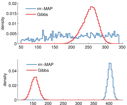
Figure 1: Empirical densities obtained by the rrr-MAP sampler (Algorithm 1) and Gibbs sampling from two different RBMs. In both cases, 10,000 samples are drawn. Top: the MNIST-trained RBM of Salakhutdinov & Murray (2008). Bottom: a random RBM, with parameters sampled independently from a standard Gaussian.

4 Experiments

Although our techniques are intended for general use with MRFs, we focus entirely on RBMs in experiments. Doing so is motivated by special interest (largely owed to uses in feature learning) and for sake of comparison with other sampling-based inference techniques. The bipartite architecture of RBMs also nicely accommodates Gibbs-based samplers. Indeed, the RBM setting proves to be challenging for relaxation and rounding to do better than Gibbs variants.

An RBM with visible variables $v\in\{-1,1\}^{m}$ and hidden variables $h\in\{-1,1\}^{p}$ fits into the above MRF framework by taking $n=m+p$ and $x=(v,h)\in\{-1,1\}^{n}$. Suppose the RBM score is

$$v^{\mathsf{T}}Wh+a^{\mathsf{T}}v+b^{\mathsf{T}}h.$$ (16)

In MRF notation, we would add a single auxiliary variable and take the augmented parameter matrix $A$ as per (14):

$$A=\frac{1}{2}\begin{bmatrix}0&a^{\mathsf{T}}&b^{\mathsf{T}}\\ a&0&W^{\mathsf{T}}\\ b&W&0\end{bmatrix}.$$ (17)

Our experiments focus on two inference scenarios: (a) approximately and efficiently computing the MAP, and (b) estimating the log-partition function $\log\sum_{v,h}p_{A}(v,h)$. The latter is discussed and motivated by Salakhutdinov & Murray (2008), and is generally interesting as it captures the essential theoretical hardness of RBM inference (Long & Servedio, 2010).

4.1 MAP inference

In these benchmarks we attempt to find a low-energy configuration $x$. We run Algorithm 1 to obtain many samples and output the best among them. We compare to an annealed Gibbs sampling procedure and to an off-the-shelf IQP solver (Gurobi) that directly optimizes (2).

We compare techniques across the following three RBM instances. Results appear in Table 1, and Figure 2 illustrates convergence.

• MNIST. We downloaded the weights for an RBM over the $\{0,1\}^{n}$ domain, trained by Salakhutdinov & Murray (2008) to model the MNIST dataset distribution. The original model has $W\in\mathbb{R}^{784\times 500}$ and we reduced it to an RBM over the $\{-1,1\}^{n}$ domain as per Section 2.3.

• Random. We populate $W\in\mathbb{R}^{784\times 500}$, $a$, and $b$ with independently random entries sampled from a standard Gaussian.

• Hard. We begin with the same type of random instance, then randomly select three pairs of variables, each of the form $(v_{i},h_{j})$ — i.e. one visible and one hidden. We modify $W_{i,j}$ to be very large (namely, 5000) and take $a_{i}$ and $b_{j}$ to be an order of magnitude smaller (i.e. 500). This construction is intended to impede a Gibbs sampler by introducing local energy minima. If we initialize such a pair at $v_{i}=h_{j}=-1$, then a Gibbs procedure is discouraged from ever flipping the value of either $v_{i}$ or $h_{j}$ conditioned on the other being $-1$.

	rrr	AG	rrr-AG	Gu
MNIST	340.29	377.47	377.39	319.34
Random	22309	22175	23358	12939
Hard	40037	36236	41016	23347

Table 1: RBM scores found by different methods: rrr is the rrr-MAP sampler (Algorithm 1); AG is an annealed Gibbs procedure with a linear temperature schedule; rrr-AG is the annealed Gibbs procedure initialized at samples obtained from rrr-MAP; Gu is the Gurobi IQP solver. Executions of rrr-MAP use $\mathsf{LRP}_{2}$ as the initial relaxation (i.e. width $k=2$). Gurobi is given an execution time limit that is 10x that of rrr.

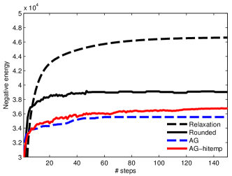
Figure 2: RBM score measured across procedure steps. The steps are qualitatively comparable: Gibbs requires a matrix-vector multiplication at every step, and $\mathsf{LRP}_{k}$ requires a gradient update (dominated by matrix-vector multiplication) and projection onto the $L_{2}$ ball (i.e. vector normalization). Black curves show the relaxed objective and the value of the best rounded sample out of a thousand. Blue and red curves show annealed Gibbs, where red is annealing starting from a 10x higher temperature.

	True	AIS	rrr-low	rrr-IS
MNIST	-	436.37	436.69	438.40
Random-S	5127.6	5127.5	5095.7	5092.4
Random-L	-	9750.5	9547.7	9606.7

Table 2: Estimates of the RBM log-partition function $\log Z(A)$: True is the true value, when available; AIS is estimation by annealed importance sampling; rrr-low is a lower bound provided by the log-sum-exp of the energy of 10K configurations obtained by the rrr-MAP sampler; rrr-IS is estimation by importance sampling using the rrr-MAP sampler as a proposal distribution. Random-S indicates small $W\in\mathbb{R}^{784\times 15}$. Random-L indicates $W$ of the same size as MNIST ($784\times 500$). In these trials, AIS was run for just under twice the amount of time as rrr-low.

4.2 Estimating the log-partition function

The goal of these trials is to estimate

$$\log Z(A)=\log\sum_{v,h}\exp(v^{\mathsf{T}}Wh+a^{\mathsf{T}}v+b^{\mathsf{T}}h).$$ (18)

The true log-partition function of large RBM instances (e.g. MNIST) is typically unknown, so we also compare results across small instances, where the true value of $\log Z(A)$ can be computed via exhaustive enumeration.

Throughout these benchmarks, we take advantage of the bipartite property of RBMs to perform an analytic summation over one class of variables. For instance, for a fixed $v$, we can analytically sum out $h$ in linear time:

$$Z(A)=\sum_{v}\exp(a^{\mathsf{T}}v)\prod_{i}\left(1+\exp(v^{\mathsf{T}}W_{i}+b_{i})\right).$$ (19)

We compare the following three estimation techniques. Results are shown in Table 2.

• Annealed importance sampling. The procedure of Salakhutdinov & Murray (2008).

• rrr-MAP sampling. 10,000 rrr-MAP samples $\{x^{(t)}\}$ are taken, and the value $\log(\sum_{t}\exp({x^{(t)}}^{\mathsf{T}}Ax^{(t)}))$ is reported. This is a lower bound on the true value of $\log Z(A)$.

• rrr-MAP importance sampling. Importance sampling using rrr-MAP sampler as a proposal distribution. 10,000 rrr-MAP samples are taken and weighted by $1/p_{X}(x)$ (as in (15)) to approximate $Z$. That is, we compute

  $$Z(A)\approx\mathbf{E}_{x\sim p_{X}}\left[\frac{\exp(x^{\mathsf{T}}Ax)}{p_{X}(x)}\right]$$ (20)

  by estimating the right hand side with an empirical mean. Note that (20) is indeed a rough approximation as $p_{X}$ has support that, for smaller $k$, is very sparse in $\{-1,1\}^{n}$. Using $k=2$, $p_{X}(x)$ can be computed in time $O(n)$ after a single $O(n\log n)$ preprocessing step.

It is expected that sampling near the MAP (as in rrr-MAP) would help in this estimation task whenever $\log Z(A)$ is dominated by a few near-MAP samples. As results show, this is perhaps a poor assumption, and further research is needed to make rrr-MAP sampling useful to this end. The method does, however, remain simple to implement, relatively efficient, and overall still comparable in estimation quality.

5 Conclusion

We described an approximate MRF inference technique based on relaxation and randomized rounding, and showed that in the RBM setting it fares comparably to more common sampling-based methods. When seeking approximate MAP configurations, it succeeds in settings where annealed Gibbs is impeded by local optima. We showed that rrr-MAP solutions can be used to initialize local search algorithms to yield better results than either technique finds alone.

The rrr-MAP algorithm is just as applicable more generally in MRFs, where Gibbs sampling is less efficient than it is in the bipartite (RBM) case. This general setting and its surrounding theory are examined in ongoing work.

References

- Alon & Naor (2006) Alon, N. and Naor, A. Approximating the cut-norm via grothendieck’s inequality. SIAM Journal on Computing, 35(4):787–803, 2006.
- Briët et al. (2010) Briët, J., de Oliveira Filho, F. M., and Vallentin, F. The positive semidefinite grothendieck problem with rank constraint. In Automata, Languages and Programming, pp. 31–42. Springer, 2010.
- Burer & Monteiro (2005) Burer, S. and Monteiro, R. Local minima and convergence in low-rank semidefinite programming. Mathematical Programming, 103(3):427–444, 2005.
- Goemans & Williamson (1995) Goemans, M. and Williamson, D. Improved approximation algorithms for maximum cut and satisfiability problems using semidefinite programming. Journal of the ACM (JACM), 42(6):1115–1145, 1995.
- Hinton (2010) Hinton, G. A practical guide to training restricted boltzmann machines. Technical report, University of Toronto, 2010.
- Long & Servedio (2010) Long, P. and Servedio, R. Restricted boltzmann machines are hard to approximately evaluate or simulate. In Proceedings of the 27th International Conference on Machine Learning, pp. 703–710, 2010.
- Nesterov (1998) Nesterov, Y. Semidefinite relaxation and nonconvex quadratic optimization. Optimization methods and software, 9(1-3):141–160, 1998.
- Ravikumar & Lafferty (2006) Ravikumar, P. and Lafferty, J. Quadratic programming relaxations for metric labeling and markov random field map estimation. In Proceedings of the 23rd international conference on Machine learning, pp. 737–744, 2006.
- Salakhutdinov & Murray (2008) Salakhutdinov, R. and Murray, I. On the quantitative analysis of deep belief networks. In Proceedings of the 25th international conference on Machine learning, pp. 872–879, 2008.