Equivalence of two Bochkov-Kuzovlev equalities in quantum two-level systems

Abstract

We present two kinds of Bochkov-Kuzovlev work equalities in a two-level system that is described by a quantum Markovian master equation. One is based on multiple time correlation functions and the other is based on the quantum trajectory viewpoint. We show that these two equalities are indeed equivalent. Importantly, this equivalence provides us a way to calculate the probability density function of the quantum work by solving the evolution equation for its characteristic function. We use a numerical model to verify these results.

Introduction. In the past decade, extending classical fluctuation relations Evans93 ; Gallavotti95 ; Kurchan98 ; Lebowitz99 ; Bochkov77 ; JarzynskiPRL97 ; Crooks99 ; HatanoSasa01 ; Maes03 ; SeifertPRL05 ; Speck05 ; Kawai07 ; EspositoPRL10 into nonequilibrium quantum regime is attracting intensive interest Bochkov77 ; Kurchanquantum ; Tasaki00 ; Yukawa00 ; PiechocinskaPRA00 ; MukamelPRL03 ; DeRoeck04 ; TalknerJPA07 ; TalknerPRE07 ; AndrieuxPrl08 ; Crooks08 ; Esposito09 ; Deffer11 ; Campisi11 ; CampisiPTRS11 ; Hekking13 ; Horowitz12 ; Leggio13 ; Mazzola13 ; Dorner13 . In the literature, the quantum measurement Kurchanquantum ; Tasaki00 ; TalknerJPA07 ; TalknerPRE07 ; Campisi11 and the quantum trajectory in Hilbert space Carmichael93 ; Breuer02 ; Wiseman10 ; Plenio98 ; Esposito09 ; DeRoeck04 ; Horowitz12 ; Hekking13 ; Leggio13 are two widely used fundamental concepts. As an alternative to those two concepts, very recently, Chetrite and Mallick Chetrite12 , and we LiuFPRE12 showed that, in the isolated Hamiltonian system and some quantum Markovian master equations (QMME) Breuer02 ; Carmichael02 , the quantum work equalities Bochkov77 ; JarzynskiPRL97 can be derived based on the time-reversal and quantum Feynman-Kac formulas. In contrast with the conventional work equalities written as statistical average of exponential functions Esposito09 ; DeRoeck04 ; Horowitz12 ; Hekking13 ; Leggio13 , which we name them the c-number equalities, the newly obtained equalities that are named the q-number equalities are remarkable analogies with their classical counterparts LiuFPRE12 ; Chetrite12 . Even so, in the case of the QMMEs, the exact relationship of the q-number and c-number equalities, and whether the q-number equalities are useful besides their forms have not been seriously considered. In this Rapid communication, we use a driven quantum two-level system (TLS) with dissipation to prove that, the q-number and the c-number Bochkov-Kuzovlev equalities (BKE) are indeed equivalent for a specific class of QMMEs. An important consequence of this investigation is that we find an efficient way to calculate the probability density function (pdf) of the quantum work for these systems without doing the quantum jump simulation Breuer02 ; Wiseman10 .

Driven quantum two-level system. The TLS has a free Hamiltonian $H_{0}$$=$$\hbar\omega\sigma_{z}/2$. Initially, the system is in the thermal state $\rho_{0}$$=$$\exp(-\beta H_{0})/{\rm Tr}[\exp(-\beta H_{0})]$ and $\beta$ is the inverse temperature of the surrounding heat reservoir. After time 0, a driving field is applied on the system up to the final time $T$. During the whole process, we assume that the evolution equation of the reduced density matrix of the system $\rho(t)$ is

$$\partial_{t}\rho(t)=L_{t}\rho(t)=-\frac{i}{\hbar}[H_{0}+H_{1}(t),\rho(t)]+D[\rho(t)],$$ (1)

where $H_{1}(t)$ is the interaction energy of the system and the driving field and we do not need to specify its concrete expression now. The time-independent term $D$ represents the dissipation due to the interaction between the TLS and the heat bath, which is

$$D[\rho(t)]=\gamma_{\downarrow}(\sigma_{-}\rho\sigma_{+}-\frac{1}{2}\{\rho,\sigma_{+}\sigma_{-}\})+\gamma_{\uparrow}(\sigma_{+}\rho\sigma_{-}-\frac{1}{2}\{\rho,\sigma_{-}\sigma_{+}\}),$$ (2)

where the two damping rates satisfy the detailed balance condition Breuer02 ,

$$\gamma_{\uparrow}=\gamma_{\downarrow}\exp(-\beta\hbar\omega).$$ (3)

This condition ensures that the system relaxes to the thermal state $\rho_{0}$ if we switch off $H_{1}(t)$. Equation (1) represents a class of QMMEs, in which the coupling of the driving field to the system and the bath is weak Bloch56 ; Redfield57 ; Geva ; Breuer97 ; Breuer04 ; Szczygielski ; Slichter ; Carmichael02 . We must point out that, the model is distinct from those in previous work DeRoeck04 ; Esposito09 ; Chetrite12 ; Horowitz12 : if one fixes the driving field at some value, the TLS may relax to some steady state but generally not to the thermal state $\propto\exp[-\beta(H_{0}+H_{1})]$. The superoperator $D$ possesses an important property Spohn78 :

$$D[A\rho_{0}]=D^{\star}[A]\rho_{0},$$ (4)

where the dual of $D$ is

$$D^{\star}[A]=\gamma_{\downarrow}(\sigma_{+}A\sigma_{-}-\frac{1}{2}\{A,\sigma_{+}\sigma_{-}\})+\gamma_{\uparrow}(\sigma_{-}A\sigma_{+}-\frac{1}{2}\{A,\sigma_{-}\sigma_{+}\}).$$ (5)

Q-number BKE. Following the spirit of establishing the classical work equalities LiuFJPA10 ; LiuFPRE09 ; Chetrite08 , we first introduce the time-reversed process $\tilde{\rho}(s)$ of Eq. (1). Its master equation is

$$\partial_{s}\tilde{\rho}(s)=\tilde{L}_{s}\tilde{\rho}(s)=-\frac{i}{\hbar}[H_{0}+\tilde{H}_{1}(s),\tilde{\rho}(s)]+D[\tilde{\rho}(s)],$$ (6)

where $H_{0}$ is time-reversible, $\tilde{H}_{1}(s)$$=$$\Theta H_{1}(t^{\prime})\Theta^{-1}$ with $t^{\prime}$=$T$$-$$s$, and $\Theta$ is time-reversal operator. We specifically set up the initial condition of the reversed process to be $\rho_{0}$. The next step is to obtain a solution for the operator $R(t^{\prime},T)$ which is defined as

$$\tilde{\rho}(s)=\Theta R(t^{\prime},T)\rho_{0}\Theta^{-1}.$$ (7)

$R(t^{\prime},T)$ indicates the deviation of the perturbed system from the equilibrium state $\rho_{0}$. Obviously, $R$$(T,T)$ is the identity operator $I$. Substituting Eq. (7) into Eq. (6) and using the relationship (4), we obtain an equation of motion for $R(t^{\prime},T)$ with respect to $t^{\prime}$:

$$\partial_{t^{\prime}}R(t^{\prime},T) = -L^{\star}_{t^{\prime}}R(t^{\prime},T)-R(t^{\prime},T)\hskip 2.84544pt\frac{i}{\hbar}[H_{1}(t^{\prime}),\hskip 2.84544pt\rho_{0}]{\rho_{0}}^{-1}$$ (8)

$$= -L^{\star}_{t^{\prime}}R(t^{\prime},T)-{\cal W}_{t^{\prime}}R(t^{\prime},T),$$ (9)

where $L_{t^{\prime}}^{\star}$ is the dual of $L_{t^{\prime}}$ Breuer02 . We also introduced the superoperator ${\cal W}_{t}$. Its action on an operator is a multiplication from the right-hand side of the operator. Using the celebrated Dyson series, Eq. (8) has the following formal solution LiuFarxiv12 ; Chetrite12 :

$$R(t^{\prime},T)=[G^{\star}(t^{\prime},T)+\sum_{n=1}^{\infty}\int_{t^{\prime}}^{T}dt_{1}\cdots\int_{t_{n-1}}^{T}dt_{n}\prod_{i=1}^{n}G^{\star}(t_{i-1},t_{i}){\cal W}_{t_{i}}G^{\star}(t_{n},T)]R(T,T),$$ (10)

where $G^{\star}(t_{1},t_{2})$$=$${\cal T}_{+}\exp[\int_{t_{1}}^{t_{2}}d\tau L^{*}_{\tau}$] $(t_{1}$$<$$t_{2})$ is the adjoint propagator of the system, and ${\cal T}_{+}$ denotes the antichronological time-ordering operator. Notice that $G^{\star}(t_{1},t_{2})(I)$$=$$I$ Breuer02 .

Equation (7) has a trivial property, i.e., the traces of its both sides being 1. Hence, substituting Eq. (10) and letting $t^{\prime}$$=$$0$, we obtain the q-number BKE:

$$1 = {\rm Tr}[R(0,T)\rho_{0}]=1+\int_{0}^{T}dt_{1}{\rm Tr}[(\frac{i}{\hbar}[H_{1}(t_{1}),\rho_{0}]\rho_{0}^{-1})G(t_{1},0)(\rho_{0})]$$

$$+\int_{0}^{T}dt_{1}\int_{t_{1}}^{T}dt_{2}{\rm Tr}[(\frac{i}{\hbar}[H_{1}(t_{2}),\rho_{0}]\rho_{0}^{-1})G(t_{2},t_{1})(\frac{i}{\hbar}[H_{1}(t_{1}),\rho_{0}]\rho_{0}^{-1}G(t_{1},0)(\rho_{0}))]+\cdots$$ (11)

$$= 1+\int_{0}^{T}dt_{1}\langle(\frac{i}{\hbar}[H_{1}(t_{1}),\rho_{0}]\rho_{0}^{-1})\rangle+\int_{0}^{T}dt_{1}\int_{t_{1}}^{T}dt_{2}\langle(\frac{i}{\hbar}[H_{1}(t_{2}),\rho_{0}]\rho_{0}^{-1})(\frac{i}{\hbar}[H_{1}(t_{1}),\rho_{0}]\rho_{0}^{-1})\rangle+\cdots$$

$$= \langle\hskip 2.84544pt{\cal T}_{+}\exp(\int_{0}^{T}d\tau\frac{i}{\hbar}[H_{1}(\tau),\rho_{0}]\rho_{0}^{-1})\hskip 2.84544pt\rangle,$$

where $G(t_{2},t_{1})$$=$${\cal T}_{-}\exp[\int_{t_{1}}^{t_{2}}d\tau L_{\tau}]$ is the system’s propagator from time $t_{1}$ to $t_{2}$, and ${\cal T}_{-}$ denotes the chronological time-ordering operator. We have used the property ${\rm Tr}[G^{\star}(t_{1},t_{2})(A)B]={\rm Tr}[AG(t_{2},t_{1})(B)]$ Breuer02 . We denote the form of the right-hand side of Eq. (Equivalence of two Bochkov-Kuzovlev equalities in quantum two-level systems) the quantum Feynman-Kac formula Chetrite12 ; LiuFPRE12 . We must remind the reader that the notation $\langle$$\cdots$$\rangle$ or the “average” above is a shorthand of the multi-time correlation functions of the operators Breuer02 . In the absence of the dissipation term $D$, Eq (Equivalence of two Bochkov-Kuzovlev equalities in quantum two-level systems) reduces into the quantum BKE for the isolated Hamiltonian system CampisiPTRS11 ; LiuFPRE12 . Moreover, if we interpret $-i[\cdots]/\hbar$ as Poisson bracket, the density matrixes as distribution functions, and the propagators under classical meaning, Eq. (Equivalence of two Bochkov-Kuzovlev equalities in quantum two-level systems) then becomes the classical BK equality Bochkov77 ; Jarzynskicmp ; LiuFJPA10 ; HorowitzJSM07 . It is worthy emphasizing that the concrete formulas of $H_{0}$ and $D$ are not involved in the above discussion.

C-number BKE. On the basis of the theory of quantum jump trajectory, we may obtain an alternative quantum BK equality comment1 . Since the basic idea and techniques have been given previously Esposito09 ; Hekking13 ; DeRoeck04 ; Crooks08 , here we only present the essential ingredients. According to the theory Carmichael93 ; Plenio98 ; Wiseman10 ; Breuer02 , the state vector $\psi(t)$ of the reduced TLS system evolves in its Hilbert space by deterministic continuous evolution and stochastic jumps alternatively. The deterministic equation is

$$\partial_{t}\psi(t) = -\frac{i}{\hbar}\hat{H}(t)\psi(t)=-\frac{i}{\hbar}[H_{0}+H_{1}(t)-\frac{i}{2}\hbar(\gamma_{\downarrow}\sigma_{+}\sigma_{-}+\gamma_{\uparrow}\sigma_{-}\sigma_{+})]\psi(t).$$ (12)

The equation has a formal solution, $\psi(t)$$=$$U(t,t_{1})\psi(t_{1})/\|\psi(t_{1})\|^{2}$, where the non-unitary time evolution operator $U(t,t_{1})$ is ${\cal T}_{-}\exp[-\frac{i}{\hbar}\int_{t_{1}}^{t}d\tau\hat{H}(\tau)].$ Occasionally, this evolution is interrupted by a stochastic jump to one of the states: $\sigma_{+}\psi(t)/\|\sigma_{+}\psi(t)\|^{2}$ and $\sigma_{-}\psi(t)/\|\sigma_{-}\psi(t)\|^{2}$. For the TLS these are the excited state $|e\rangle$ and ground state $|g\rangle$, respectively. In the quantum optics, these jumps appear an absorbtion or emission of a photon Carmichael93 ; Wiseman10 ; Breuer02 ; Plenio98 . Hence, the corresponding energy could be physically interpreted as heat absorbed or released by the system from or to the heat bath Hekking13 ; Horowitz12 ; DeRoeck04 ; Crooks08 ; Esposito09 . By measuring the energy of the TLS at the beginning time ($\epsilon_{n}$) and ending time ($\epsilon_{m}$) while recording the number $N_{+}$ ($N_{-}$) of the jumps to $|e\rangle$ ($|g\rangle$) along a quantum trajectory, we define the work done by the driving field on the TLS as

$$W=\epsilon_{n}-\epsilon_{m}-\omega\hbar\int_{0}^{T}dN_{+}+\omega\hbar\int_{0}^{T}dN_{-},$$ (13)

where $dN_{+}$ and $dN_{-}$ are the increments of these two types of jumps. We remind the reader that the first two terms are the energy eigenvalues of the free Hamiltonian $H_{0}$ instead of the total Hamiltonian. With the above notations, we give the c-number BKE for the quantum work (13):

$$1 = \sum_{m,n}p_{m}(0)\sum_{N=0}^{\infty}\int_{0}^{T}\cdots\int_{t_{N-1}}^{T}\prod_{1}^{N}dt_{i}\sum_{\gamma_{1}}\cdots\sum_{\gamma_{N}}[\hskip 2.84544pt\prod_{1}^{N}\gamma_{i}\left|\langle n|{\cal L}_{N}|m\rangle\right|^{2}\hskip 2.84544pt]\hskip 5.69046pte^{-\beta W}=E[e^{-\beta W}],$$ (14)

where $p_{m}(0)$ $=$ $\exp(-\beta\epsilon_{m})/{\rm Tr}[\exp(-\beta H_{0})]$ is the initial probability of the TLS at the eigenstate with the energy $\varepsilon_{m}$, the whole term inside the square brackets of the first equation is the probability density of observing a quantum trajectory that starts from the eigenstate $|m\rangle$, occurs jump at time $t_{i}$ with type $P_{i}$ that equals $\sigma_{+}$ or $\sigma_{-}$ with the jump rate $\gamma_{i}$=$\gamma_{\uparrow}$ or $\gamma_{\downarrow}$ ($i$$=$$1$,$\cdots$,$N$), and ends in the eigenstate $|n\rangle$ at the final time $T$, and

$${\cal L}_{N}=U(T,t_{N})P_{N}\cdots U(t_{2},t_{1})P_{1}U(t_{1},0)$$ (15)

is the time evolution operator of the whole trajectory Breuer02 . We specifically use the notation $E[\cdots]$ to denote the average in the c-number equality. Proof of the equality will be seen shortly.

Equivalence of the two BKEs. Although we name Eq. (Equivalence of two Bochkov-Kuzovlev equalities in quantum two-level systems) the BKE, its physical relevance is not obvious. We do not see from the abstract equality what the work is and whether the second law of thermodynamics is implied. It is quite different from the c-number BKE (14). At first glance, these two equalities appear so distinct. However, we will show that it is only superficial. Before the summation over $m$, Eq. (14) can be rewritten as

$$p_{m}(0)\sum_{n}\sum_{N=0}^{\infty}\int_{0}^{T}\cdots\int_{t_{N-1}}^{T}\prod_{1}^{N}dt_{i}\sum_{\gamma_{1}}\cdots\sum_{\gamma_{N}}[\hskip 2.84544pt\prod_{1}^{N}\tilde{\gamma_{i}}\left|\langle m|{\hskip 2.84544pt}{\cal L}_{N}^{\dagger}|n\rangle\right|^{2}\hskip 2.84544pt]\hskip 5.69046pte^{-\beta W}e^{-\beta(\hbar\omega N_{+}-\hbar\omega N_{-})}$$ (16)

$$= \langle m|\hskip 1.42271pt\Theta^{-1}\sum_{n}p_{n}(0)\sum_{N=0}^{\infty}\int_{0}^{T}\cdots\int_{s_{N-1}}^{T}\prod_{1}^{N}ds_{i}\sum_{\tilde{\gamma}_{1}}\cdots\sum_{\tilde{\gamma}_{N}}\hskip 2.84544pt\prod_{1}^{N}{\tilde{\gamma}}_{i}\hskip 2.84544pt\tilde{{\cal L}}_{N}\hskip 2.84544pt\Theta|n\rangle\langle n|\Theta^{-1}\hskip 2.84544pt\tilde{{\cal L}}_{N}^{\dagger}\hskip 2.84544pt\Theta|m\rangle$$

$$= \langle m|\Theta^{-1}\tilde{\rho}(T)\hskip 2.84544pt\Theta|m\rangle,$$

where $\tilde{\gamma}_{\downarrow}$$=$$\gamma_{\uparrow}$, $\tilde{\gamma}_{\uparrow}$$=$$\gamma_{\downarrow}$, $s_{i}$$+$$t_{N+1-i}$$=$$T$,

$$\tilde{{\cal L}}_{N}=\tilde{U}(T,s_{N})P_{1}^{\dagger}\cdots\tilde{U}(s_{2},s_{1})P_{N}^{\dagger}\tilde{U}(s_{1},0)$$ (17)

is the time evolution operator of the reversed quantum trajectory, and $\tilde{U}(s,s_{1})$ is analogous to the previous $U(t,t_{1})$ except that the Hamiltonian therein is replaced by $H_{0}$$+$$\tilde{H}_{1}(s)$. The last exponential term in the first line of Eq. (16) is the consequence of the detailed balance condition (4), and the final equation is due to the well-established relationship between the density matrix and the quantum trajectory Breuer02 ; Wiseman10 . Comparing Eq. (7) with Eq. (16), we immediately see that, the whole expression after $p_{m}(0)$ is just $\langle m|R(0,T)|m\rangle$ on the left hand side of the latter equation. Therefore, we prove that the c-number and q-number BKEs are exactly equivalent.

An alternative proof of this equivalence that does not depend on the time-reversal explanation is to do series expansions for these two BKEs in terms of $\beta$. We then compare their respective coefficients of the different orders of $\beta$. For the c-number BKE, the expansion is simply

$$1=1-E[W]\beta+\frac{1}{2}E[W^{2}]\beta^{2}\cdots.$$ (18)

Using the facts that $E[dN_{+}]$$=$$\gamma_{\uparrow}$${\rm Tr}[\sigma_{-}\sigma_{+}\rho(t)]dt$ and $E[dN_{-}]$$=$$\gamma_{\downarrow}$${\rm Tr}[\sigma_{+}\sigma_{-}\rho(t)]dt$ Breuer02 ; Wiseman10 , where $t$ is the time of non-vanishing $dN_{\pm}$, we rewrite the first moment of the work (13) as (see the Supplemental Material)

$$E[W] = \int_{0}^{T}dt_{1}\frac{d}{dt_{1}}\hskip 2.84544pt{\rm Tr}[H_{0}\rho(t_{1})]-\int_{0}^{T}dt_{1}{\rm Tr}[D^{\star}[H_{0}]\rho(t_{1})]=\int_{0}^{T}dt_{1}\langle\frac{i}{\hbar}[H_{1}(t_{1}),H_{0}]\rangle.$$ (19)

Because the left hand side is the average work and the first integration in the first equation represents a change of average energy of the TLS during the whole process, we may interpret the second integration in the same equation as the absorbed average heat from the heat bath. Hence, Eq. (19) is just the first law of thermodynamics. Using the Jensen’s inequality, we surely have the second law of thermodynamics, $E[W]\geq 0$. A more complex case is the second moment. Using the three crucial identities below comment2 ,

$$E[dN_{+}dN^{\prime}_{+}] = \{\gamma_{\uparrow}^{2}\hskip 2.84544pt{\rm Tr}[\sigma_{-}\sigma_{+}G(t,t^{\prime})(\sigma_{+}\rho(t^{\prime})\sigma_{-})]+\delta(t-t^{\prime})\gamma_{\uparrow}{\rm Tr}[\sigma_{-}\sigma_{+}\rho(t)]\}dtdt^{\prime},\hskip 5.69046pt(t\geq t^{\prime}),$$ (20)

$$E[dN_{-}dN^{\prime}_{-}] = \{\gamma_{\downarrow}^{2}\hskip 2.84544pt{\rm Tr}[\sigma_{+}\sigma_{-}G(t,t^{\prime})(\sigma_{-}\rho(t^{\prime})\sigma_{+})]+\delta(t-t^{\prime})\gamma_{\downarrow}{\rm Tr}[\sigma_{+}\sigma_{-}\rho(t)]\}dtdt^{\prime},\hskip 5.69046pt(t\geq t^{\prime}),$$ (21)

$$E[dN_{+}dN^{\prime}_{-}] = \{\gamma_{\downarrow}\gamma_{\uparrow}{\rm Tr}[\sigma_{-}\sigma_{+}G(t,t^{\prime})(\sigma_{-}\rho(t^{\prime})\sigma_{+})]\theta(t-t^{\prime})+\gamma_{\downarrow}\gamma_{\uparrow}{\rm Tr}[\sigma_{+}\sigma_{-}G(t^{\prime},t)(\sigma_{+}\rho(t)\sigma_{-})]\theta(t^{\prime}-t)\}dtdt^{\prime},$$ (22)

where $t$ ($t^{\prime}$) is the time of non-vanishing $dN_{\pm}$ ($dN^{\prime}_{\pm}$), and doing a careful calculation, we obtain

$$\frac{1}{2}E[W^{2}]=\int_{0}^{T}dt_{1}\int_{t_{1}}^{T}dt_{2}\langle(\frac{i}{\hbar}[H_{1}(t_{2}),H_{0}])(\frac{i}{\hbar}[H_{1}(t_{1}),H_{0}])\rangle-\frac{1}{2}\int_{0}^{T}dt_{1}\langle\hskip 2.84544pt[\hskip 2.84544pt\frac{i}{\hbar}[H(t_{1}),H_{0}],H_{0}]\rangle.$$ (23)

When we expand the q-number BKE (Equivalence of two Bochkov-Kuzovlev equalities in quantum two-level systems) accordingly, we find that the coefficients of $\beta$ and $\beta^{2}$ are indeed the right hand sides of Eqs. (19) and (23). Higher orders of $\beta$ can be checked analogously. But the calculation becomes very long and tedious dramatically.

Characteristic function of the work. The preceding argument about the equivalence of Eq. (Equivalence of two Bochkov-Kuzovlev equalities in quantum two-level systems) and Eq. (14) is useful. First, we may apply Eqs. (19) and (23) to calculate the first two moments of the work by analytically or numerically solving the master equations rather than by doing the quantum jump simulation. Compared with the latter, the former is exact and involves no sampling errors. As an illustration, we recalculate these moments for the TLS model in Ref. Hekking13 , where $H_{1}(t)$$=$$\lambda_{0}\sin(\omega t)(\sigma_{+}+\sigma_{-})$; see Fig. (1). The simulation data are also listed for a comparison. Second, the equivalence provides us an interesting method to calculate the pdf of the quantum work (13). Letting the characteristic function Campisi11 of the pdf be $\Phi(u)$, where $u$ is the real number, we easily see that

$$\Phi(u)=E[\hskip 1.42271pte^{iuW}]={\rm Tr}[K(0,T;u)\rho_{0}],$$ (24)

if the newly introduced operator $K(t^{\prime},T;u)$ satisfies the evolution equation given by

$$\left\{\begin{array}[]{ll}\partial_{t^{\prime}}K(t^{\prime},T;u)=-L^{\star}_{t^{\prime}}K(t^{\prime},T;u)-K(t^{\prime},T;u)\hskip 2.84544pt\frac{i}{\hbar}[H_{1}(t^{\prime}),\hskip 2.84544pte^{iuH_{0}}]e^{-iuH_{0}},&\\ K(T,T;u)=I.\end{array}\right.$$ (27)

By numerically solving the above equation and performing an inverse Fourier transform of $\Phi(u)$, the pdf of the work is then obtained. The inset of Fig. (1) is an example. We see that our calculation agrees with the simulation data Hekking13 excellently.

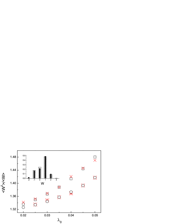
Figure 1: The ratio of the second and first moments of the quantum work (in unit $\hbar\omega$) with respect to different perturbation strength $\lambda_{0}$ (in unit $\hbar\omega$) for the TLS model in Ref. Hekking13 , where $T\omega/2\pi$$=$$10$, $\beta\hbar\omega$$=$$2.0$. The crosses ($\gamma_{\downarrow}$$=$$0.02\omega$) and stars ($\gamma_{\downarrow}$$=$$0.01\omega$) are the data of the quantum jump simulation Hekking13 , while the open squares and circles are the numerical results of Eqs. (19) and (23). The inset shows the pdf of the quantum work. The dashed bars are from the simulation of Ref. Hekking13 , and the solid black bars are obtained by our characteristic function method, where $\beta\hbar\omega$$=$$1.0$, $\gamma_{\downarrow}$$=$$0.05\omega$, $\lambda_{0}$$=$$0.05\hbar\omega$.

Conclusion. In this work, we present two kinds of BKEs in the quantum TLS driven by the field and we prove their equivalence. Moreover, an efficient way of calculating the characteristic function of the quantum work is revealed. So far, our discussions are limited to these specific QMMEs where the driven field is so weak that their dissipations can be treated as time-independent. Extending the current idea into the more general cases, e.g., the master equations with time-dependent dissipations shall be very intriguing. We expect that some of them would be related to the quantum Jarzynski equality. This study is underway.

We appreciate Prof. Hekking for permitting us to use their simulation data in Ref. Hekking13 . We also thank Prof. Jarzynski, Dr. Deffner, and Zhiyue Lu for their useful remarks on the work. This work was supported by the National Science Foundation of China under Grant No. 11174025.

I Derivations of Eqs. (19) and (23)

For Eq. (19), the situation is simple:

$$E[W] = E[\epsilon_{n}]-E[\epsilon_{m}]+\hbar\omega E[N_{+}]-\hbar\omega E[N_{-}]$$ (28)

$$= {\rm Tr}[H_{0}\rho(T)]-{\rm Tr}[H_{0}\rho(0)]+\int_{0}^{T}{\rm Tr}[\hbar\omega(\gamma_{\downarrow}\sigma_{+}\sigma_{-}-\gamma_{\uparrow}\sigma_{-}\sigma_{+})\rho(t_{1})]dt_{1}$$

$$= \int_{0}^{T}dt_{1}\frac{d}{dt_{1}}{\rm Tr}[H_{0}\rho(t_{1})]-\int_{0}^{T}dt_{1}{\rm Tr}[D^{\star}[H_{0}]\rho(t_{1})]$$

$$= \int_{0}^{T}dt_{1}{\rm Tr}[\frac{i}{\hbar}[H_{1}(t_{1}),H_{0}]\rho(t_{1})].$$

For Eq. (23), however, the proof becomes very tricky. First we write down the original definition of the second moment of the quantum work (13),

$$E[W^{2}] = E[\epsilon_{n}^{2}+\epsilon_{m}^{2}-2\epsilon_{n}\epsilon_{m}]+2\hbar\omega E[\epsilon_{n}N_{+}-\epsilon_{n}N_{-}-\epsilon_{m}N_{+}+\epsilon_{m}N_{-}]$$ (29)

$$+(\hbar\omega)^{2}E[N_{+}^{2}-2N_{+}N_{-}+N_{-}^{2}].$$

The first two averages can be rewritten using the density matrix $\rho(t)$ and the propagator $G(t_{2},t_{1})$ as

$${\rm Tr}[H_{0}^{2}\rho(T)]+{\rm Tr}[H_{0}^{2}\rho(0)]-2{\rm Tr}[H_{0}G(T,0)H_{0}\rho(0)]$$ (30)

and

$$\int_{0}^{T}dt_{1}{\rm Tr}[\gamma_{\downarrow}H_{0}G(T,t_{1})\sigma_{-}\rho(t_{1})\sigma_{+}]-\int_{0}^{T}dt_{1}{\rm Tr}[\gamma_{\uparrow}H_{0}G(T,t_{1})\sigma_{+}\rho(t_{1})\sigma_{-}]$$

$$-\int_{0}^{T}dt_{1}{\rm Tr}[\gamma_{\downarrow}\sigma_{+}\sigma_{-}G(t_{1},0)H_{0}\rho(0)]+\int_{0}^{T}dt_{1}{\rm Tr}[\gamma_{\uparrow}\sigma_{-}\sigma_{+}G(t_{1},0)H_{0}\rho(0)],$$ (31)

respectively. For the last average in Eq. (29), we have to resort to Eqs. (20)-(22) and obtain

$$2\int_{0}^{T}dt_{1}\int_{t_{1}}^{T}dt_{2}{\rm Tr}[\gamma_{\downarrow}^{2}\sigma_{+}\sigma_{-}G(t_{2},t_{1})\sigma_{-}\rho(t_{1})\sigma_{+}]+\int_{0}^{T}dt_{1}{\rm Tr}[\gamma_{\downarrow}\sigma_{+}\sigma_{-}\rho(t_{1})]$$

$$-2\int_{0}^{T}dt_{1}\int_{t_{1}}^{T}dt_{2}{\rm Tr}[\gamma_{\uparrow}\gamma_{\downarrow}\sigma_{+}\sigma_{-}G(t_{2},t_{1})\sigma_{+}\rho(t_{1})\sigma_{-}]-2\int_{0}^{T}dt_{1}\int_{t_{1}}^{T}dt_{2}{\rm Tr}[\gamma_{\downarrow}\gamma_{\uparrow}\sigma_{-}\sigma_{+}G(t_{2},t_{1})\sigma_{-}\rho(t_{1})\sigma_{+}]$$

$$+2\int_{0}^{T}dt_{1}\int_{t_{1}}^{T}dt_{2}{\rm Tr}[\gamma_{\uparrow}^{2}\sigma_{-}\sigma_{+}G(t_{2},t_{1})\sigma_{+}\rho(t_{1})\sigma_{-}]+\int_{0}^{T}dt_{1}{\rm Tr}[\gamma_{\uparrow}\sigma_{-}\sigma_{+}\rho(t_{1})].$$ (32)

Substituting Eqs. (30)-(I) into Eq. (29) and doing a rearrangement, we have

$$E[W^{2}]= 2(\hbar\omega)^{2}\int_{0}^{T}dt_{1}\int_{t_{1}}^{T}dt_{2}{\rm Tr}[(\gamma_{\downarrow}\sigma_{+}\sigma_{-}-\gamma_{\uparrow}\sigma_{-}\sigma_{+})G(t_{2},t_{1})(\gamma_{\downarrow}\sigma_{-}\rho(t_{1})\sigma_{+}-\gamma_{\uparrow}\sigma_{+}\rho(t_{1})\sigma_{-})]$$ (33)

$$+2\hbar\omega\int_{0}^{T}dt_{1}{\rm Tr}[H_{0}G(T,t_{1})(\gamma_{\downarrow}\sigma_{-}\rho(t_{1})\sigma_{+}-\gamma_{\uparrow}\sigma_{+}\rho(t_{1})\sigma_{-})]$$

$$-2\hbar\omega\int_{0}^{T}dt_{1}{\rm Tr}[(\gamma_{\downarrow}\sigma_{+}\sigma_{-}-\gamma_{\uparrow}\sigma_{-}\sigma_{+})G(t_{1},0)H_{0}\rho(0)]$$

$$+{\rm Tr}[H_{0}^{2}\rho(T)]+{\rm Tr}[H_{0}^{2}\rho(0)]-2{\rm Tr}[H_{0}G(T,0)H_{0}\rho(0)]$$

$$+(\hbar\omega)^{2}\int_{0}^{T}dt_{1}{\rm Tr}[\gamma_{\downarrow}\sigma_{+}\sigma_{-}\rho(t_{1})]+(\hbar\omega)^{2}\int_{0}^{T}dt_{1}{\rm Tr}[\gamma_{\uparrow}\sigma_{-}\sigma_{+}\rho(t_{1})].$$

At this step, we do not see that Eq. (33) essentially equals to the right hand side of Eq. (23). In order to go head, We need to introduce two additional equations:

$$L_{t}[H_{0}\rho] = H_{0}L_{t}[\rho]-\frac{i}{\hbar}[H_{1}(t),H_{0}]\rho+\hbar\omega(\gamma_{\downarrow}\sigma_{-}\rho\sigma_{+}-\gamma_{\uparrow}\sigma_{+}\rho\sigma_{-}),$$ (34)

$$L_{t}^{\star}[H_{0}H_{0}] = \frac{i}{\hbar}[H_{1}(t),H_{0}]H_{0}+\frac{i}{\hbar}H_{0}[H_{1}(t),H_{0}]+2D^{\star}[H_{0}]H_{0}+(\hbar\omega)^{2}\gamma_{\downarrow}\sigma_{+}\sigma_{-}+(\hbar\omega)^{2}\gamma_{\uparrow}\sigma_{-}\sigma_{+}.$$ (35)

Using the expression of $D^{\star}[H_{0}]$ in Eq. (28), the definition of the adjoint propagator $G^{\star}(t_{1},t_{2})$, the above two equations, and carrying out further calculations we obtain

$$\frac{1}{2}E[W^{2}]= -\int_{0}^{T}dt_{1}\int_{t_{1}}^{T}dt_{2}{\rm Tr}[D^{\star}[H_{0}]G(t_{2},t_{1})\frac{i}{\hbar}[H_{1}(t_{1}),H_{0}]\rho(t_{1})]$$ (36)

$$+\int_{0}^{T}dt_{1}{\rm Tr}[H_{0}G(T,t_{1})\frac{i}{\hbar}[H_{1}(t_{1}),H_{0}]\rho(t_{1})]$$

$$-\frac{1}{2}\int_{0}^{T}dt_{1}{\rm Tr}[\frac{i}{\hbar}[H_{1}(t_{1}),H_{0}]H_{0}\rho(t_{1})]-\frac{1}{2}\int_{0}^{T}dt_{1}{\rm Tr}[H_{0}\frac{i}{\hbar}[H_{1}(t_{1}),H_{0}]\rho(t_{1})].$$

Using the property of $G^{\star}(t_{1},t_{2})$,

$$\partial_{t_{2}}[G^{\star}(t_{1},t_{2})H_{0}]=G^{\star}(t_{1},t_{2})\frac{i}{\hbar}[H_{1}(t_{1}),H_{0}]+G^{\star}(t_{1},t_{2})D^{\star}[H_{0}],$$ (37)

we finally arrive at the right hand side of Eq. (23). Noting that $G^{\star}(t_{1},t_{2})$ is a superoperator that acts on the operator on its right hand side Breuer02 .

II Calculating $K(t^{\prime},T;u)$ for the TSL model

For the simple resonant TSL model in Ref. Hekking13 , we may write the operator $K(t^{\prime},T;u)$ in the Pauli matrixes as

$$K(t^{\prime},T;u)=\frac{1}{2}[k_{0}(t^{\prime})I+k_{x}(t^{\prime})\sigma_{x}++k_{y}(t^{\prime})\sigma_{y}+k_{z}(t^{\prime})\sigma_{z}].$$ (38)

Substituting it into Eq. (25) and doing a simple derivation, we obtain

$$\dot{k_{0}} = \frac{i}{2}e^{-iu}(e^{iu}-1)^{2}\lambda(t^{\prime})k_{x}-\frac{1}{2}e^{-iu}(e^{2iu}-1)\lambda(t^{\prime})k_{y}+(\gamma_{\downarrow}-\gamma_{\uparrow})k_{z},$$ (39)

$$\dot{k_{x}} = \frac{i}{2}e^{-iu}(e^{iu}-1)^{2}\lambda(t^{\prime})k_{0}+\frac{1}{2}(\gamma_{\downarrow}+\gamma_{\uparrow})k_{x}-\omega k_{y}+\frac{i}{2}e^{-iu}(e^{2iu}-1)\lambda(t^{\prime})k_{z},$$ (40)

$$\dot{k_{y}} = \frac{1}{2}e^{-iu}(1-e^{2iu})\lambda(t^{\prime})k_{0}+\omega k_{x}+\frac{1}{2}(\gamma_{\downarrow}+\gamma_{\uparrow})k_{y}-\frac{1}{2}e^{-iu}(1+e^{iu})^{2}\lambda(t^{\prime})k_{z},$$ (41)

$$\dot{k_{z}} = \frac{i}{2}e^{-iu}(1-e^{2iu})\lambda(t^{\prime})k_{x}+\frac{1}{2}e^{-iu}(1+e^{iu})^{2}\lambda(t^{\prime})k_{y}+(\gamma_{\downarrow}+\gamma_{\uparrow})k_{z},$$ (42)

where the dots denote the time derivative $d/d{t^{\prime}}$, $\lambda(t^{\prime})$$=$$\lambda_{0}\omega\sin(\omega t^{\prime})$, and the terminal conditions are $k_{0}(T)$$=$$2$, $k_{x}(T)$$=$$k_{y}(T)$$=$$k_{z}(T)$$=$$0$, respectively. The reader is reminded that all parameters are dimensionless. We clearly see that the operator $K$ is periodic with respect to $u$, i.e. $K(t^{\prime},T;u+2n\pi)$$=$$K(t^{\prime},T;u)$ for arbitrary integer $n$. This feature ensures that the pdf of the quantum work is discrete after we perform the inverse Fourier transform for $\Phi(u)$. These differential equations can be easily solved numerically as a terminal problem, e.g., by using the Mathematica.

III General QMMEs having structure of Eq. (1)

We have mentioned that Eq. (1) is a simplest example of the specific type of QMMEs. The dissipation parts of these QMMEs have the following common structure Breuer02

$$D[\rho]=\sum_{j}\gamma^{j}_{\downarrow}(A^{j}_{-}\rho A^{j}_{+}-\frac{1}{2}\{\rho,A^{j}_{+}A^{j}_{-}\})+\gamma^{j}_{\uparrow}(A^{j}_{+}\rho A^{j}_{-}-\frac{1}{2}\{\rho,A^{j}_{-}A^{j}_{+}\}),$$ (43)

where the Lindblad operators are the eigenoperators of the free Hamiltonian $H_{0}$, i.e., $[H_{0},A^{j}_{\pm}]$$=$$\pm\hbar\omega_{j}A^{j}_{\pm}$, and the damping rates are assumed to satisfy $\gamma^{j}_{\uparrow}$$=$$\gamma^{j}_{\downarrow}\exp(-\beta\hbar\omega_{j})$. Except for the additional summation over all possible coupling channels $j$ of the system with the heat bath, we do not see that there are fundamental differences between the generalized and the simplest QMMEs. Therefore, all general results in the main text could be simply extended into the general situation by changing $\sigma_{\pm}$$\rightarrow$$A^{i}_{\pm}$, $N_{\pm}$$\rightarrow$$N^{i}_{\pm}$, $\omega$$\rightarrow$$\omega_{i}$, $\gamma_{\downarrow\uparrow}$$\rightarrow$$\gamma^{i}_{\downarrow\uparrow}$, and doing appropriate summation over the various channels $j$, e.g., the quantum work for the QMMEs with Eq. (43) is

$$W=\epsilon_{n}-\epsilon_{m}+\sum_{j}\hbar\omega_{j}N^{j}_{+}-\sum_{j}\hbar\omega_{j}N^{j}_{-}.$$ (44)

Noting that the three Eqs. (20)-(22) are not zero only for the same channels.

References

(1) G. N. Bochkov and Yu E. Kuzovlev, Sov.
Phys. JETP 45, 125 (1977).
(2) D. J. Evans, E. G. D. Cohen, and G. P. Morriss,
Phys. Rev. Lett. 71, 2401 (1993).
(3) G. Gallavotti and E. G. D. Cohen, Phys.
Rev. Lett. 74, 2694 (1995).
(4) J. Kurchan, J. Phys. A, 31, 3719
(1998).
(5) J. L. Lebowitz and H. Spohn, J. Stat. Phys.
95, 333 (1999).
(6) C. Jarzynski, Phys. Rev. Lett. 78, 2690 (1997); Phys. Rev. E. 56, 5018 (1997).
(7) G. E. Crooks, Phys. Rev. E 60, 2721
(1999); Phys. Rev. E 61, 2361 (2000).
(8) T. Hatano and S. I. Sasa, Phys. Rev. Lett.
86, 3463 (2001).
(9) C. Maes, Sem. Poincare 2, 29 (2003).
(10) U. Seifert, Phy. Rev. Lett. 95,
040602 (2005).
(11) T. Speck and U. Seifert, J. Phys. A 38,
L581 (2005).
(12) R. Kawai, J. M. R Parrondo, and C. Van den
Broeck, Phys. Rev. Lett. 98, 080602 (2007).
(13) M. Esposito and C. Van den Broeck, Phys. Rev. Lett. 104, 090601 (2010).
(14) B. Piechocinska, Phys. Rev. A 61, 062314 (2000).
(15) J. Kurchan, arXiv: cond-mat/0007360 (2000).
(16) S. Yukawa, J. Phys. Soc. Jpn. 69, 2367
(2000).
(17) H. Tasaki, arXiv:cond-mat/0009244 (2000).
(18) S. Mukamel, Phys. Rev. Lett. 90,
170604 (2003).
(19) W. De Roeck and C. Maes, Phys. Rev. E 69, 026115 (2004).
(20) P. Talkner, E. Lutz, and P. Hänggi,
Phys. Rev. E 75, 050102 (2007).
(21) P. Talkner and P. Hänggi, J.
Phys. A 40, F569 (2007).
(22) D. Andrieux and P. Gaspard, Phys. Rev.
Lett. 100, 230404 (2008).
(23) G. E. Crooks, Phys. Rev. A, 77, 034101
(2008).
(24)M. Esposito, U. Harbola and S. Mukamel, Rev.
Mod. Phys. 81, 1665 (2009).
(25) S. Deffner and E. Lutz, Phys. Rev. Lett. 107,
140404 (2011).
(26) M. Campisi, P. Talkner, and P. Hänggi,
Phil. Trans. R. Soc. A 369, 291 (2011).
(27) M. Campisi, P. Hänggi, and P. Talkner,
Rev. Mod. Phys. 83, 771 (2011).
(28) J. M. Horowitz, Phys. Rev. E 85,
031110 (2012).
(29) B. Leggio, A. Napoli, A. Messina, and H. P.
Breuer, Phys. Rev. A88, 042111 (2013).
(30) F. W. J. Hekking and J. P. Pekola, Phys. Rev.
Lett. 111, 093602 (2013).
(31) L. Mazzola, G. De Chiara, and M. Paternostro, Phys. Rev. Lett. 110, 230602 (2013).
(32) R. Dorner, S. R. Clark, L. Heaney, R. Fazio, J. Goold, and V.
Vedral, Phys. Rev. Lett. 110, 230601 (2013).
(33) H. J. Carmichael, An open systems approach to quantum optics (Springer, Berlin, 1993).
(34) H. P. Breuer and F. Petruccione, The Theory of Open Quantum Systems (London: Oxford University
Press, 2002).
(35) M. B. Plenio and P. L. Knight, Rev. Mod. Phys. 70, 101 (1998).
(36) H. M. Wiseman and G. J. Milburn, Quantum Measurement and Control
(Cambridge Univ. Press, 2010).
(37) R. Chetrite and K. Mallick, J. Stat. Phys. 148, 480 (2012).
(38) F. Liu, Phys. Rev. E 86, 010103(R) (2012).
(39) F. Bloch, Phys. Rev. 102, 104 (1956).
(40) A. G. Redfield, IBM J. 19, 1 (1957).
(41) C. Slichter, Principles of Magnetic Resonance (Springer-Verlag, Berlin,
1990).
(42) E. Geva, R. Kosloff, and J. L. Skinner, J. Chem.
Phys. 102, 8541 (1995).
(43) H. P. Breuer and F. Petruccione, Phys. Rev. A
55, 3101 (1997).
(44) H. P. Breuer, Phys. Rev. A
70, 012106 (2004).
(45) K. Szczygielski, D. Gelbwaser-Klimovsky,
and R. Alicki, Phys. Rev. E 87, 012120 (2013).
(46) H. J. Carmichael, Two-Level Atoms and Spontaneous
Emission (Springer, Berlin, 2002).
(47) H. Spohn and J. L. Lebowitz, Adv. Chem. Phys. 38, 109 (1978).
(48) R. Chetrite and K. Gawedzki, Commun. Math.
Phys. 282, 469 (2008).
(49) F. Liu and Z. C. Ou-Yang, Phys. Rev. E
79, 060107(R) (2009).
(50) F. Liu, H. Tong, R. Ma and Z. C. Ou-Yang, J.
Phys. A: Math. Theor. 43, 495003 (2010).
(51) F. Liu, arXiv: 1210.5798v1 (2012).
(52) C. Jarzynski, C. R. Physique, 8, 495 (2007).
(53) J. Horowitz, C. Jazynski, J. Stat. Mech:
Theory Exp. P11002 (2007).
(54) Hekking and Pekola should first present the
c-number BKE Hekking13 . However, they claimed that they
verified the quantum Jarzynski equality. Compared with the method
developed in this work, Their method is relatively complex.
(55) These equations are the generalizatoins of
Eq. (4.50) in the book of Wiseman and Milburn Wiseman10 .