Broken SU(4) symmetry in a Kondo-correlated carbon nanotube

Abstract

Understanding the interplay between many-body phenomena and non-equilibrium in systems with entangled spin and orbital degrees of freedom is a central objective in nano-electronics. We demonstrate that the combination of Coulomb interaction, spin-orbit coupling and valley mixing results in a particular selection of the inelastic virtual processes contributing to the Kondo resonance in carbon nanotubes at low temperatures. This effect is dictated by conjugation properties of the underlying carbon nanotube spectrum at zero and finite magnetic field. Our measurements on a clean carbon nanotube are complemented by calculations based on a new approach to the non-equilibrium Kondo problem which well reproduces the rich experimental observations in Kondo transport.

I Introduction

The Kondo effect Kondo (1964) is an archetypical manifestation of strong electronic correlations in mesoscopic systems. While first observed in bulk metals with ferromagnetic impurities, it was shown to lead to a distinct zero-bias anomaly in the differential conductance of semiconductor quantum dots with odd electronic occupation Goldhaber-Gordon et al. (1998a, b); Cronenwett et al. (1998). A degeneracy of quantum states required for its occurrence is usually provided by the electronic spin degree of freedom, resulting in the so-called $SU(2)$ Kondo behavior. Remarkably, in the Kondo regime the differential conductance obeys universal scaling as a function of temperature Goldhaber-Gordon et al. (1998b), bias voltage Grobis et al. (2008), and magnetic field Gaass et al. (2011).

Clean carbon nanotubes (CNTs) Cao et al. (2005) provide a unique test-bed for the investigation and manipulation of the quantum dot level structure and its consequences for the Kondo effect Nygård et al. (2000). In CNTs an additional degeneracy in the intrinsic low energy spectrum stems from two (K, K’) graphene Dirac points and enables one to study unconventional correlation phenomena such as the orbital $SU(2)$ as well as spin plus orbital $SU(4)$ Kondo effects both experimentally Jarillo-Herrero et al. (2005); Makarovski et al. (2007) and theoretically Borda et al. (2003); Choi et al. (2005); Lim et al. (2006); Fang et al. (2008a, 2010); Lim et al. (2011); Galpin et al. (2010). Besides revealing the curvature induced spin-orbit interaction Kuemmeth et al. (2008); Del Valle et al. (2011); Steele et al. (2013); Ando (2000), experiments indicate that also the K-K’ degeneracy is frequently lifted with a finite energy $\Delta_{\text{KK'}}$ Kuemmeth et al. (2008); Jespersen et al. (2011); Grove-Rasmussen et al. (2012). While usually attributed to the presence of disorder in damaged or contaminated CNTs, it is observed also in clean carbon nanotubes as a contribution from the CNT’s contact interfaces Marganska et al. (2014).

In the following, we demonstrate how this type of $SU(4)$ symmetry breaking leads to unconventional Kondo transport phenomena. Our results clearly show that the Kondo behavior at zero magnetic field is controlled by time reversal symmetry, which allows to identify two distinct, two-fold degenerate Kramers doublets. The analysis of the breaking of this symmetry in a magnetic field parallel ($B_{\parallel}$) or perpendicular ($B_{\perp}$) to the CNT axis leads to a detailed understanding of the many-body processes contributing to transport in the Kondo regime. It allows to disentangle the role of the conjugation relations and goes significantly beyond earlier studies on Kondo ions Garnier et al. (1997); Reinert et al. (2001); Ernst et al. (2011), where Kondo satellites could be observed but the tunability of the spectrum by a magnetic field was not given.

As discussed below, our studies also significantly advance the understanding of Kondo physics in CNTs in the deeply non perturbative regime. In particular, we elucidate the reasons for the absence of certain many-body transitions expected from previous theoretical works Fang et al. (2008a, 2010); Lim et al. (2011) but not observed in our as well as in previous experiments Quay et al. (2007); Lan et al. (2012); Cleuziou et al. (2013).

II Transport measurements

Electronic transport measurements have been performed on a clean, freely suspended single-wall carbon nanotube (CNT) contacted with rhenium and capacitively coupled to a global back gate at milli-Kelvin temperatures. The carbon nanotube was grown by chemical vapor deposition across pre-defined trenches and electrode structures to minimize damage and contamination mechanisms Kong et al. (1998); Cao et al. (2005).

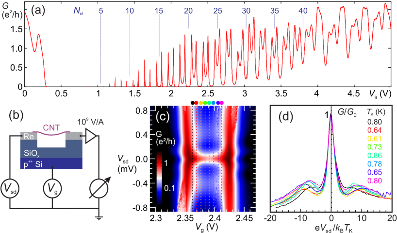
Figure 1: (Color) Measurement of the Kondo effect in transport through an ultra-clean carbon nanotube. (a) Low-bias conductance ($V_{\text{sd}}=0.2{\,\text{mV}}$) through a clean, suspended small band gap carbon nanotube as function of applied gate voltage $V_{\text{g}}$. (b) Device geometry and electronic measurement setup for differential conductance measurement. (c) Differential conductance $G(V_{\text{g}},V_{\text{sd}})={\,\text{d}}I(V_{\text{g}},V_{\text{sd}})/{\,\text{d}}V_{\text{sd}}$ inside and around the gate voltage window with $N_{\text{el}}=21$ ($T=30{\,\text{mK}}$). A sharp Kondo ridge at zero bias voltage $V_{\text{sd}}=0$ and broader satellite ridges at finite bias $V_{\text{sd}}\simeq\pm 0.5{\,\text{mV}}$ are clearly visible. (d) Line traces $G(V_{\text{sd}})$ at constant $V_{\text{g}}$ corresponding to colored dotted lines in (c), with $V_{\text{sd}}$ rescaled by the corresponding Kondo temperature $T_{\text{K}}$ (see text). The central conductance peak at $V_{\text{sd}}=0$ displays the universal Kondo behavior, while the satellite peaks move. A similar plot across different Coulomb oscillations can be found in the Appendix, Fig. 13.

As seen in the low-bias conductance (Fig. 1(a)), a small band gap separates a Fabry-Pérot pattern Liang et al. (2001) in the highly transparent hole regime from sharp Coulomb blockade oscillations in the few electron regime ($N_{\text{el}}<10$). With increasing gate voltage enhanced conductance is observed, leading in particular to a Kondo zero-bias anomaly in the odd electron number valleys. The electronic setup used for the measurements is sketched in Figure 1(b). A dc- and an ac-voltage are superimposed and applied as bias voltage $V_{\text{sd}}=V_{\text{sd}}^{\text{dc}}+V_{\text{sd}}^{\text{ac}}$ to the source contact. The current from the drain contact is converted to a voltage and measured with a lock-in amplifier. The highly positive doped silicon substrate acts as global back gate.

In the following, we focus on the intermediate coupling regime and measure the differential conductance as a function of gate voltage $V_{\text{g}}$ and bias voltage $V_{\text{sd}}$ (Figure 1(c)). Besides the pronounced conductance ridge at zero bias voltage, additional broad satellite peaks appear symmetrically at finite bias voltage $V_{\text{sd}}\simeq\pm 0.5{\,\text{mV}}$, depending only weakly on the gate voltage. In analogy to the case of a broken spin degeneracy in a magnetic field, these satellite peaks at zero magnetic field signal a lifted degeneracy of the ground state, allowing inelastic transport processes to take place. Finite bias conductance peaks together with a zero bias Kondo peak have already been observed in CNT quantum dots with odd shell filling Nygård et al. (2000); Quay et al. (2007); Lan et al. (2012); Cleuziou et al. (2013). In the latter three experiments the evolution of the satellites in perpendicular Quay et al. (2007) and parallel Lan et al. (2012); Cleuziou et al. (2013) magnetic fields have been reported. Because a finite field breaks time reversal symmetry, inelastic transitions between Zeeman splitted or orbitally splitted levels are expected to become visible Jespersen et al. (2011); Fang et al. (2008a). Strikingly, in the three experiments Quay et al. (2007); Lan et al. (2012); Cleuziou et al. (2013) not all of the inelastic transitions expected from (possibly Kondo enhanced) cotunneling Jespersen et al. (2011) or for the non perturbative Kondo regime Fang et al. (2008a) could be seen. In this work we clarify the nature of the transitions contributing to the finite bias peaks.

Non-equilibrium co-tunneling is a threshold effect which can give rise to a step-like cusp in the differential conductance Wegewijs and Nazarov (2001). Kondo correlations treated within lowest order perturbation theory yield a logarithmic enhancement of this cusp which emphasizes further the threshold effect Paaske et al. (2006). This behavior is expected in the perturbative regime $T>T_{\text{K}}$ of temperatures larger than the Kondo temperature. In the strong coupling regime $T<T_{\text{K}}$ a perturbative treatment of Kondo correlations is no longer appropriate. At such low temperatures, and for $k_{\rm B}T_{K}\sim\Delta$, where $\Delta$ is the energy of the inelastic transition associated to valley mixing and spin-orbit coupling, true Kondo peaks at finite bias, rather than co-tunneling cusps, are expected to develop Fang et al. (2008a); Galpin et al. (2010). This is the parameter regime in Quay et al. (2007); Lan et al. (2012); Cleuziou et al. (2013) and, as demonstrated below, also of our experiments. Hence, the conductance traces in Figure 1(d) are a manifestation of the Kondo effect in the strong coupling regime. As we shall show, the interplay of Coulomb interaction and the intrinsic symmetry properties of the CNT-Hamiltonian yields a selective enhancement of virtual processes contributing to the Kondo effect in the non perturbative regime.

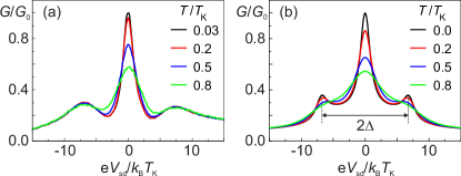
Figure 2: (Color online) Temperature dependence of the main Kondo resonance and its satellites. (a) Measured differential conductance traces $G(V_{\text{sd}})$ at different temperatures, normalized by $G_{0}=G(V_{\text{sd}}=0)$ for the lowest temperature at $V_{\text{g}}=2.39{\,\text{V}}$; the bias voltage is scaled with the Kondo temperature $T_{\text{K}}=0.86{\,\text{K}}$. (b) Differential conductance obtained from our field-theoretical calculation. The distance between the satellite peaks at $T=0$ used in the calculation is $2\Delta=13.8\,k_{\text{B}}T_{\text{K}}$.

III Universality

To unambiguously claim that a zero-bias anomaly observed in experiments has Kondo origin, the characteristic universal scaling behavior with the energy scale determined by the Kondo temperature $T_{\text{K}}$ has to be tested. We record conductance traces $G(V_{\text{sd}})$ at different discrete gate voltage values $V_{\text{g}}$ within the $21^{\text{st}}$ Coulomb diamond. For each such trace, we determine the Kondo temperature $T_{\text{K}}(V_{\text{g}})$ in non-equilibrium from the central peak in the bias voltage trace using the condition $G(k_{\text{B}}T_{\text{K}}/e)\simeq 2G_{0}/3$ and $G_{0}=G(V_{\text{sd}}=0)$ Kretinin et al. (2012); Pletyukhov and Schoeller (2012). We then rescale the bias voltage with the respective Kondo temperature, and normalize the conductance to its maximum value $G_{0}\sim 0.5e^{2}/h$. The collapse of all curves $G(eV_{\text{sd}}/k_{\text{B}}T_{\text{K}})/G_{0}$ around $V_{\text{sd}}=0$ into universal behavior, as illustrated in Fig. 1(d), clearly demonstrates the Kondo origin of the zero-bias feature. This behavior can be compared with the theoretical curves in Fig. 9, where we show that the universal line shape of the central Kondo resonance remains essentially unchanged also in the transition between $SU(2)$ and $SU(4)$.

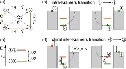
Figure 3: (Color online) Conjugation relations, level spectrum, and selected Kondo transport processes. (a) Energy levels associated with a longitudinal mode of a CNT accounting for spin and valley degrees of freedom. The time-reversal operator $\hat{\mathcal{T}}$ connects the states $(1,2)$ and $(3,4)$. The operators $\hat{\mathcal{C}}$ and $\hat{\mathcal{P}}$ govern chiral and particle-hole conjugation and provide further pairs of conjugated states. Chiral pairs are $(1,3)$ and $(2,4)$; particle-hole pairs are $(1,4)$ and $(2,3)$. (b) Spin-orbit coupling and valley mixing break the four-fold degeneracy but not the time-reversal symmetry. The spectrum splits in two degenerate Kramers doublets $(1,2)$ and $(3,4)$, respectively, separated by the energy difference $\Delta=\sqrt{{\Delta_{\text{KK'}}}^{2}+{\Delta_{\text{SO}}}^{2}}$. (c) The Kondo peak at zero bias is governed by virtual processes within the Kramers pairs $(1,2)$ and $(3,4)$ (intra-Kramers transitions). (d) The satellite peaks at finite bias, $V_{\text{sd}}=\pm\Delta/e$, result from inelastic transitions within the chiral pairs, $(1,3)$ and $(2,4)$ (chiral inter-Kramers transitions).

After the rescaling the position of the satellite peaks varies, i.e., here the universality is apparently lost. This is to be expected since the Kondo temperature $T_{\text{K}}$ varies within the Coulomb valley region but the splitting $\Delta$ between central peak and satellites is gate independent. Complete universality of the differential conductance, i.e., universality in the whole range of voltages, requires the ratio $\Delta/k_{\text{B}}T_{\text{K}}$ to be invariant Yamada et al. (1984). In general one obtains $T_{\text{K}}(\Delta)=T_{\text{K}}(0)f[\Delta/k_{\rm B}T_{\text{K}}(0)]$, where $T_{\text{K}}(0)=T_{\text{K}}^{SU(4)}$ is the Kondo temperature for the $SU(4)$ Kondo effect, and $f(x)$ depends on the strength of the $SU(4)$ symmetry breaking. In our experiment we find $\Delta/k_{\text{B}}T_{\text{K}}\simeq 7$. As shown in Ref. Galpin et al. (2010), this implies that in our experiment the $SU(4)$ symmetry is weakly broken.

Finally, we notice a nonmonotonic dependence of $T_{\text{K}}$ on the gate voltage $V_{\text{g}}$, with a local maximum in the center of the Coulomb blockade region. Such behavior is not expected for the $SU(2)$ Anderson model, which rather predicts a local minimum Schrieffer and Wolff (1966). Hence, the peculiar voltage dependence observed in our experiment may as well be a signature of weakly broken $SU(4)$.

IV Temperature dependence

Figure 2(a) displays the temperature dependence of $G(V_{\text{sd}},T)$ in the center of the same Coulomb diamond ($N_{\text{el}}=21$), where $V_{\text{g}}=2.39\,{\,\text{V}}$. The central peak behaves in a way characteristic for the Kondo effect: it is suppressed and broadened for increasing temperatures. The satellite peaks are increasingly washed out at elevated temperatures. A slight bias asymmetry is observed in the curves, which we attribute to asymmetries in the couplings to the leads. Such asymmetries are also responsible for the reduction of the maximum $G_{0}$ with respect to the unitary limit value $2e^{2}/h$ expected for a fully symmetric set-up.

Figure 2(b) displays the differential conductance obtained from our calculation based on the slave boson Keldysh effective action formalism Altland and Simons (2010) discussed in Sec. VII and in the Appendix. The calculation uses the minimal model Hamiltonian Eq. (3) for a single longitudinal mode of a CNT including spin orbit interaction (with the energy scale $\Delta_{\text{SO}}$) and valley mixing (with characteristic energy scale $\Delta_{\text{KK'}}$). These couplings break the orbital degeneracy of the CNT spectrum (and hence the $SU(4)$ symmetry) but preserve time-reversal symmetry. As a result, the non interacting CNT spectrum displays two degenerate Kramers doublets separated by the spacing $\Delta=\sqrt{{\Delta_{\text{KK'}}}^{2}+{\Delta_{\text{SO}}}^{2}}$. The simulation uses the value of $2\Delta=13.8k_{\rm B}T_{\text{K}}$ obtained from the experiment. For simplicity, and to stress the universal features of the problem, a symmetric coupling to the leads has been used in the simulation, as well as equal coupling of the CNT modes to the leads. Hence, in our calculation the central peak reaches at zero temperature the unitary limit $2e^{2}/h$. To compare with the experiment, the theoretical curves have been normalized by the maximum theoretical value $G_{0}=2e^{2}/h$. Our calculation reproduces well the experimentally observed evolution of peak amplitudes with temperature. The tails at high voltages decay faster than in the experiment. This behavior is due to our approximation scheme for the Keldysh effective action, where only terms quadratic in the slave bosonic fields are retained. Within this approximation, the behavior of the central and inelastic peaks has been proven to be accurately reproduced for the $SU(2)$ Anderson model Smirnov and Grifoni (2013a, b). To improve the description of the tails quartic terms should be included. Such treatment, however, would go beyond the scope of this work.

V Conjugation relations

A quantitative analysis of our experimental results has to combine the properties of the underlying set of single-particle states with the Kondo-correlations. In this section we analyze conjugation relations valid for the single particle spectrum which turn out to have significant impact on the many-body properties of our CNT quantum dot. In the simplest model for a CNT one expects a four-fold degenerate longitudinal level at the energy $\varepsilon_{d}$ Laird et al. (2014). This degeneracy is removed by KK’ valley mixing and spin-orbit interaction with splitting $\Delta$. We denote the four resulting energies associated to the eigenstates $|1\rangle,|2\rangle,|3\rangle,|4\rangle$ by $\varepsilon_{1},\varepsilon_{2},\varepsilon_{3},\varepsilon_{4}$, respectively. At zero magnetic field, the effective CNT-Hamiltonian $\hat{H}^{(0)}_{\text{CNT}}$ (see Eq. (3) in the Appendix) displays time-reversal (TR) symmetry governed by the operator $\hat{\mathcal{T}}$. The ${\mathcal{T}}$-conjugated pairs of states are the Kramers doublets $(1,2)$ and $(3,4)$, with $\varepsilon_{1}=\varepsilon_{2}$, and $\varepsilon_{3}=\varepsilon_{4}=\varepsilon_{1}-\Delta$, see Fig. 3(a). Additional operators $\hat{\mathcal{P}}$ and $\hat{\mathcal{C}}$ can be introduced, which anticommute with $\hat{H}^{(0)}_{\text{CNT}}$ and which allow to connect the states within one quadruplet in the way depicted in Fig. 3(a) (see Appendix A for further details). We call the operations related to $\hat{\mathcal{P}}$ and $\hat{\mathcal{C}}$ particle-hole (PH) Altland and Zirnbauer (1997); foo and chiral (C) conjugation, respectively. The operator $\hat{\mathcal{P}}$ conjugates states from different Kramers doublets; the pairs are $(1,4)$ and $(2,3)$ with $\varepsilon_{1}(\Delta)=\varepsilon_{d}+\Delta/2=\varepsilon_{4}(-\Delta)$, and $\varepsilon_{2}(\Delta)=\varepsilon_{d}+\Delta/2=\varepsilon_{3}(-\Delta)$, as displayed in Fig. 3(b). If TR and PH conjugation hold, so does chiral conjugation, which is represented by the operator $\hat{\mathcal{C}}=\hat{\mathcal{P}}\hat{\mathcal{T}}^{-1}$. The chirally conjugated pairs are $(1,3)$ and $(2,4)$.

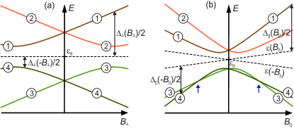
Figure 4: (Color online) Sketch of the evolution of the energy levels in a magnetic field (a) perpendicular and (b) parallel to the CNT axis in the parameter regime ${\Delta_{\text{KK'}}}>{\Delta_{\text{SO}}}$. The energy eigenstates are labeled $1-4$. At $B=0$ there are two energy degenerate Kramers doublets $(1,2)$ and $(3,4)$. At finite fields the degeneracy is lifted and the conjugation relations $\varepsilon_{1}(\vec{B})=\varepsilon_{2}(-\vec{B})$ and $\varepsilon_{3}(\vec{B})=\varepsilon_{4}(-\vec{B})$ hold. (a) In perpendicular field the energy difference within each chiral pair, i.e., $(1,3)$ and $(2,4)$, remains essentially independent of $B_{\perp}$, provided that $B_{\perp}\lesssim{\Delta_{\text{KK'}}}/g_{\text{s}}\mu_{\text{B}}$. Moreover, the particle-hole pairs $(1,4)$ and $(2,3)$ are related by the conjugation relations $\varepsilon_{1}(\Delta_{\perp}(B_{\perp}))=\varepsilon_{d}+\Delta_{\perp}(B_{\perp})/2=\varepsilon_{4}(-\Delta_{\perp}(B_{\perp}))$ and $\varepsilon_{2}(\Delta_{\perp}(-B_{\perp}))=\varepsilon_{d}+\Delta_{\perp}(-B_{\perp})/2=\varepsilon_{3}(-\Delta_{\perp}(-B_{\perp}))$. b) For $B_{\parallel}$ the Aharonov-Bohm effect induces a level crossing of the pair $(3,4)$, as indicated by the blue arrows. Again $\mathcal{P}$-conjugation holds. E.g., for the pair $(1,4)$ we find the relation $\varepsilon_{1}(B_{\parallel},\Delta_{\parallel}(B_{\parallel}))=\varepsilon(B_{\parallel})+\Delta_{\parallel}(B_{\parallel})/2=\varepsilon_{4}(B_{\parallel},-\Delta_{\parallel}(B_{\parallel}))$.

The zero-bias Kondo peak is necessarily induced by transitions between the degenerate states of the time-reversed Kramers pairs $(1,2)$ and $(3,4)$, which we call ’intra-Kramers’ transitions, see Fig. 3(c). A similar reasoning applies for the finite bias Kondo peaks at voltages equal to $\pm\Delta/e$: the inelastic peaks are necessarily induced by transitions between distinct Kramers pairs, called in the following ’inter-Kramers transitions. From Figs.  2(a) and (b) no further information on the nature of the inelastic transitions can be extracted.

Additional insight can be obtained by looking at the evolution of the central peak and of its satellites in finite magnetic fields, as TR is broken and hence Kramers degeneracy is lifted. Figure 4(a) and 4(b) display the dispersion of the four single particle states in a magnetic field perpendicular and parallel to the tube axis. It is clearly visible that in a finite magnetic field, $\vec{B}$, conjugation relations persist that lead to close connections between the single particle energies, e.g. $\hat{\mathcal{T}}|1,\vec{B}\rangle=|2,-\vec{B}\rangle$ leads to $\varepsilon_{1}(\vec{B})=\varepsilon_{2}(-\vec{B})$, and $\hat{\mathcal{P}}|1,\vec{B}\rangle=|4,\vec{B}\rangle$ leads to $\varepsilon_{1}(\vec{B},\Delta(\vec{B}))=\varepsilon_{4}(\vec{B},-\Delta(\vec{B}))$, with $\Delta(\vec{B})$ being a magnetic field dependent level splitting (see Eqs. (25), (26) and (27) of Appendix A).

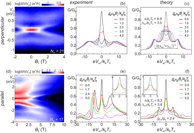
Figure 5: (Color) Kondo differential conductance in a magnetic field. (a) Measured differential conductance $G(B_{\perp},V_{\text{sd}})$ as a function of the bias voltage $V_{\text{sd}}$ and magnetic field $B_{\perp}$ perpendicular to the CNT axis at $V_{\text{g}}=2.39\,{\,\text{V}}$ corresponding to the electron number $N_{\text{el}}=21$. The central peak splits at $B_{\perp}>0.7\,k_{\text{B}}T_{\text{K}}/g_{\text{s}}\mu_{\text{B}}$, while the satellites remain nearly unaffected. (b) Line traces $G(V_{\text{sd}})$ versus bias voltage (rescaled with $T_{\text{K}}=0.86{\,\text{K}}$) from (a) for several values of $B_{\perp}$. (c) Theoretical results for the differential conductance at zero temperature for corresponding values of $g_{\text{s}}\mu_{\text{B}}B_{\perp}/k_{\text{B}}T_{\text{K}}$ showing good agreement with the experiment not . (d) Measurement as in (a) but in parallel alignment of the magnetic field, $G(B_{\parallel},V_{\text{sd}})$, $N_{\text{el}}=17$. (e) Line traces from (d), where $V_{\text{sd}}$ is scaled with the Kondo temperature $T_{\text{K}}=1.12{\,\text{K}}$ and the conductance is scaled using its maximum $G_{0}=G(V_{\text{sd}}=0)$ at $B_{\parallel}=0{\,\text{T}}$. (f) Theoretical results for the differential conductance at zero temperature for different values of $B_{\parallel}$. The insets in (e) and (f) show the evolution of the central peak in the experiment and theory, respectively.

As revealed by the evolution of the satellite peaks in magnetic field shown in the next section, they only involve transitions among the chiral pairs $(1,3)$ and $(2,4)$ [see Fig. 3(d)], while transitions between ${\mathcal{P}}$-conjugated states are absent. Our observations seem to be consistent with other data in the non perturbative regime shown in Quay et al. (2007); Lan et al. (2012); Cleuziou et al. (2013). Also in those experiments no ${\mathcal{P}}$-transitions could be resolved in finite magnetic fields. For example, in the experiment by Cleuziou et al., Ref. Cleuziou et al. (2013), only one of the two expected excitation lines (called $\beta$ and $\delta$ by the authors) could be identified, see Fig. 2(a) in Ref. Cleuziou et al. (2013). Using the parameters given in that paper, we find that the non-observed inelastic transition is $\delta$, corresponding in our terminology to a $\mathcal{P}$-transition.

VI Evolution of the Kondo peaks in magnetic field

The behavior of the Kondo peaks in magnetic field, reported in Figs. 5 and 6, provides a sensitive tool that allows us to discriminate between the different types of Kondo-enhanced transitions. In fact, the positions of the Kondo peaks are related to the energy differences between the two dot states involved in the transition, and these depend very differently on direction and strength of the magnetic field for transitions between ${\mathcal{T}}$, ${\mathcal{C}}$, or ${\mathcal{P}}$ pairs. The central Kondo peak results from intra-Kramers transitions and its splitting reveals the breaking of time reversal symmetry. From the Keldysh effective action theory (see Sec. VII) a splitting of the central Kondo resonance is expected once the energetic separation within a Kramers doublet exceeds a threshold value $\varepsilon_{\text{c}}$, as observed in Figs. 5(a),(b) and 5(d),(e).

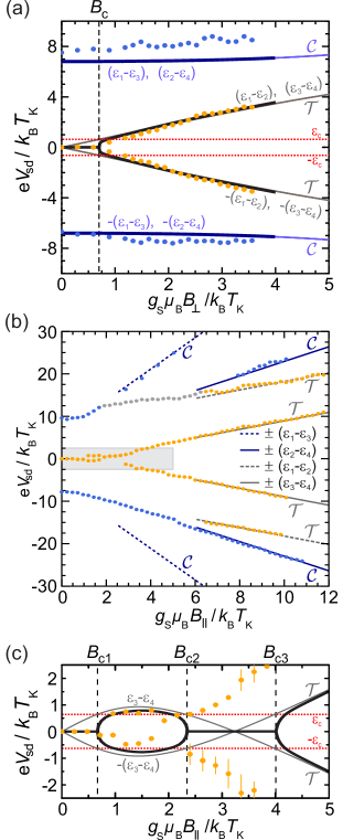
Figure 6: (Color) Magnetic field behavior of the Kondo peaks. (a) Predicted evolution of the Kondo peaks in perpendicular field taking into account many-body effects (thick solid lines) together with single particle energy differences (thin solid lines) and the experimental data (dots). A splitting occurs when the energy difference within the lowest Kramers doublet $|\varepsilon_{3}-\varepsilon_{4}|$ exceeds $\varepsilon_{\text{c}}$. (b) Experimental evolution of the Kondo peaks in parallel magnetic field (dots), compared with single-particle energy differences (solid and dashed lines) evaluated at large fields. The grey rectangle identifies the low field and low bias region analyzed in panel (c). (c) Evolution of the low-bias Kondo peaks in parallel magnetic field. In this case $\delta_{\parallel,1}=|\varepsilon_{3}-\varepsilon_{4}|$ (grey solid line) first grows with increasing field until it exceeds the threshold $\varepsilon_{\text{c}}$ (red dotted line) at the critical field $B_{\text{c1}}$, beyond which the peak starts to split (see dots and thick solid line). The predicted peak splitting vanishes again at $B_{c2}$. Above $B_{c3}$ it grows again, first in a sublinear way and afterwards linearly with the magnetic field.

In perpendicular fields puzzling at first glance is the independence of the positions of the satellite Kondo peaks on the field [Figs. 5(a),(b)]. This is in strong contrast to the co-tunneling regime investigated earlier (see Fig. 3 in Ref. Jespersen et al., 2011), where a splitting of the inelastic co-tunneling line was observed as a result of two possible sets of transitions: within the pair $(4,2)$ or $(4,1)$ for positive, and within pair $(3,1)$ or $(3,2)$ for negative field orientation [cf. Fig. 4(b)]. In our case only the transitions between the ${\mathcal{C}}$-conjugated states, $(4,2)$ and $(3,1)$, are observed while the transitions between the ${\mathcal{P}}$-conjugated states, $(4,1)$ and $(3,2)$, are absent. This observation substantiates the previous experimental report in Quay et al. (2007), and is in nearly perfect agreement with the results of our many-body theory plotted in Fig. 5(c). No Kondo-enhancement of the virtual transitions (4,1) and (3,2) occurs as a consequence of the symmetry constraints imposed onto the Keldysh action discussed in the following Sec. VII. These constraints reduce the allowed number of Kondo peaks expected in a perpendicular magnetic field with respect to earlier theoretical predictions (cf. Refs. Fang et al. (2008a, 2010)).

In magnetic fields parallel to the tube axis the satellite Kondo peaks are expected to move and split because, according to Figs. 4(b),(c), the single particle states 2 and 4 (1 and 3) are mutually tilted by the Aharonov-Bohm effect. Inspection of Figs. 5(d) and 5(e) shows that the Kondo satellites now depend on the magnetic field, in qualitative agreement with our theoretical result displayed in Fig. 5(f). Note that the following parameters of our model Hamiltonian are extracted from the experimental data: the ratio $\Delta/k_{\text{B}}T_{\text{K}}$ (see Fig. 2), and the ratio ${\Delta_{\text{SO}}}/k_{\text{B}}T_{\text{K}}$, which are obtained from the evolution of the splitted central Kondo peaks according to Eqs. (28) and (41), respectively. For the parallel field case only, also the ratio $g_{\text{orb}}/g_{\text{s}}$ of orbital and spin $g$-factor has to be set. The parameters used to generate the theoretical curves in Figs. 5(c) and 5(f) are given in Table 2 of Appendix A.

In order to better identify which transitions contribute to the evolution of the central peaks and of the satellites at finite magnetic fields, we compare the maxima of the $G(V_{\text{sd}})$ traces [orange, blue and grey dots in Fig. 6] with the results of the many body theory and the energy differences of the underlying single particle levels [thick and thin lines in Fig. 6, respectively]. Orange and blue dots correspond to transitions that, according to theory, are of the ${\mathcal{T}}$- and ${\mathcal{C}}$-type, respectively. To the grey dots no clear assignment can be made . Noticeably, only transitions of the ${\mathcal{T}}$- and ${\mathcal{C}}$-type are seen. A careful inspection of the second derivative of the $I(V_{\text{sd}})$ confirms that the lines corresponding to transitions between ${\mathcal{P}}$-conjugated states are indeed absent in the experiment. The absence of a splitting of the satellite peaks in the perpendicular field is very prominent in Fig. 6(a), where the position of the satellite peaks is essentially free of dispersion. On the other hand, the satellite peaks do split in a parallel magnetic field, where the Aharonov-Bohm effect acts differently on the two pairs of ${\mathcal{C}}$-conjugated states as seen in Fig. 6(b). The high field behavior observed here is similar to that in Lan et al. (2012), and confirms the absence of $\mathcal{P}$-transitions reported there. An additional discussion of the evolution of the conductance peaks can be found in Appendix C.

Finally, we focus on the critical behavior of the central Kondo peaks in a magnetic field $\vec{B}$. A single Kondo peak is expected as long as the level separation of the underlying single particle states does not exceed the threshold value $\varepsilon_{\text{c}}$. The threshold value $\varepsilon_{\text{c}}$ (dotted red lines in Fig. 6(a), (c)) defines one critical magnetic field $B_{\text{c}}=0.6\,k_{\text{B}}T_{\text{K}}/g_{\text{s}}\mu_{\text{B}}$ for the perpendicular, and three critical fields $B_{\text{c1}}$ – $B_{\text{c3}}$ for the parallel field direction. This characteristic difference arises from the additional crossing of the single particle levels 3 and 4 near $k_{\text{B}}T_{\text{K}}/g_{\text{s}}\mu_{\text{B}}\simeq 3.3{\,\text{T}}$ in Fig. 4(b), see also Ref. Jespersen et al. (2011). Results of our many-body calculations (thick lines in panels (a) and (c)) well match our experiment in perpendicular and in low parallel magnetic fields. The non-linear dispersion of the positions of the central Kondo peaks reflects the protection of the Kondo state against perturbations on energy scales below $k_{\text{B}}T_{\text{K}}$.

VII Modeling and nonlinear transport theory

To account for the striking findings in magnetic field, we have developed a nonequilibrium field theory based on the slave boson Keldysh effective action formalism Altland and Simons (2010). An $SU(2)$ formulation of this theory has been presented in Refs. Smirnov and Grifoni (2013a, b) and an $SU(4)$ formulation (including a broken $SU(4)$) is presented in this work in Appendix B. The theory is based on the minimal model Hamiltonian $\hat{H}_{\text{CNT}}$ for a single longitudinal mode of a CNT quantum dot in magnetic field as given in Eq. (2) of the Appendix. Accounting for the four eigenstates $\left\{|j\rangle,~{}j=1,2,3,4\right\}$ of $\hat{H}_{\text{CNT}}$, the Coulomb interaction among them, and assuming a tunneling coupling which preserves CNT quantum numbers, the theory provides an approximate analytical expression for the four contributions $\nu_{j}(\varepsilon)$ to the tunneling density of states (TDOS) of the quantum dot. This expression is then used to evaluate the differential conductance as a function of the temperature, bias voltage and magnetic field over the whole energy range relevant for Kondo physics according to the Meir-Wingreen formula Wingreen and Meir (1994), cf. Eq. (59) of the Appendix.

To explicit calculate $\nu_{j}(\varepsilon)$, the interacting CNT Hamiltonian is first expressed in terms of slave bosons and fermions. The fermions in the tube and in the leads are then integrated out, leaving a still exact expression for $\nu_{j}(\varepsilon)$ in terms of the Keldysh effective action, see Eq. (61) and (68), which only depends on the slave boson fields. In the limit of infinite charging energy, they represent fluctuations of the empty state of the dot. The bosonic fields cannot be integrated out exactly as the tunneling term of the Keldysh action, Eq. (62), is nonlinear in them. Crucially though, this tunneling action is constructed in a such a way that for each CNT level $i$ there are two expansion points ($\gamma_{i}$ and $\delta_{i}$ in Eqs. (64), (65), respectively). Upon expanding the action around the expansion points and retaining only quadratic terms, each $\nu_{j}$ is readily obtained by functional integration over the slave bosonic fields.

The essence of the Kondo physics is the enhancement of certain virtual transitions when going towards low energies. In the perturbative regime the enhancement is only logarithmic. Thus one expects that all the transitions (independent of whether they are logarithmically enhanced or not) should be experimentally accessible by inelastic cotunneling spectroscopy (see e.g. Jespersen et al. (2011)). In the low energy non perturbative regime the enhancement is much larger, as it yields resonances on the order of $e^{2}/h$. Thus, it is only in the latter regime that the lack of enhancement of some transitions clearly appears. A commonly used approach to determine which transitions are enhanced is to solve flow equations for the associated coupling constants in an effective Kondo model, see e.g. Refs. Paaske et al. (2006); Lim et al. (2006) for an application to CNTs. As outlined above, in the Keldysh approach one is not solving flow equations for the coupling constants. Rather, the evolution towards low energies is controlled by the expansion points $\gamma_{i}$ and $\delta_{i}$ in the effective Keldysh action. The expansion points $\gamma_{i}$ and $\delta_{i}$ are free parameters of the theory. Their value is fixed $a\ posteriori$ by imposing the proper low energy behavior of the total TDOS as known e.g. from Fermi liquid theory exp . Additionally, they are fixed in such a way that conjugation relations for the single particle spectrum are reflected in analogous conjugation relations among the $\nu_{j}$. Notice that for each $\nu_{j}$ the four complex quantities $E_{i}^{j}=\gamma_{i}^{j}\delta_{i}^{j}$ have to be determined.

For the $SU(2)$ Anderson model at zero magnetic field, time reversal symmetry requires $\nu_{1}=\nu_{2}$ ($j=1,2$ for the two spin degenerate levels). Hence, $E_{i}^{j}=E\;\forall\;i,j=1,2$. Then, the value of the complex quantity $E$ is uniquely fixed by constraints on the tunneling density of states and its derivative at zero temperature and at the Fermi energy known from Fermi liquid theory. A very good agreement of the theory with equilibrium numerical renormalization group results and with out of equilibrium real-time renormalization group predictions was demonstrated over the whole parameter regime Smirnov and Grifoni (2013a). To account for the effects of finite magnetic fields, a spin dependence of the expansion points must be included. In Ref. Smirnov and Grifoni (2013b) the choice was dictated by the observation that a) the flow towards energies requires virtual spin-flip processes (see e.g. Altland and Simons (2010)), and b) conjugation relations among the magnetic field splitted single particle levels should also be reflected at the level of the TDOS, i.e. $\nu_{1}(B)=\nu_{2}(-B)$. According to a) and b), the choice of the expansion points is such that each of the two contributions $\nu_{1}$ and $\nu_{2}$ effectively contains (through the related self-energy) only virtual spin-flip processes. This together with the Fermi liquid conditions on the TDOS at zero field uniquely determines the value of the expansion points. The merit of this choice has to be checked against other theories or experimental findings. As shown in Ref. Smirnov and Grifoni (2013b) (cf. Fig. 3 there), the theory well reproduces the experimentally observed evolution of the split Kondo peaks in a magnetic field seen in Ref. Quay et al. (2007). However, it does not quantitatively describe the tails of the Zeeman split peaks, as some inelastic cotunneling contributions are not retained in the second order expansion of the effective action.

A similar reasoning is applied in this work. Due to the presence of orbital and spin degrees of freedom, the total TDOS is the sum of the four contributions $\nu_{j}(\varepsilon)$, one for each of the four levels. For each $\nu_{j}$, the expansion points of the Keldysh effective action, i.e. the real and imaginary parts of the four $E^{j}_{i}$ are chosen according to the requirement that a) virtual processes that flip the quantum number are crucial for the low energy behavior Choi et al. (2005); Lim et al. (2006), b) the TDOSs should be related by conjugation relations inherited from the single particle spectrum reflecting $\mathcal{T}$- and $\mathcal{P}$-conjugation in finite magnetic field:

$$\nu_{1}(\vec{B})=\nu_{2}(-\vec{B}),\quad\nu_{3}(\vec{B})=\nu_{4}(-\vec{B}),\quad\nu_{1}(\Delta)=\nu_{4}(-\Delta),$$ (1)

where $\Delta(\vec{B})$ is the magnetic field dependent inelastic energy introduced in Sec. V. These requirements, and the $SU(4)$ limit at zero field $\vec{B}$ and zero splitting $\Delta$, $uniquely\ fix$ the expansion points at low energies. One crucial consequence of the combined quantum number flip and conjugations requirement, is that the TDOS $\nu_{j}$ effectively only contains (through its self-energy $\Sigma_{j}$) virtual transitions to the $\mathcal{T}$ and $\mathcal{C}$-conjugated partners of the level $j$, but not to the $\mathcal{P}$-conjugated ones. The explicit form for the $E_{i}^{j}$, $\nu_{j}$, and $\Sigma_{j}$ is given in Eqs. (69), (70), and (72) in the Appendix.

VIII Conclusion

In conclusion, our work provides a systematic experimental and theoretical investigation of the Kondo effect in carbon nanotubes in the presence of both spin-orbit coupling and valley mixing. The wide tunability of the carbon nanotube spectrum by magnetic fields allows to elucidate the role of symmetry and conjugation relations. Despite the symmetry breaking by spin-orbit interaction and valley mixing, the underlying operators still give rise to conjugation relations between certain states that have to be respected by the transport theory. The interplay of electron-electron interactions and conjugation relations lead to the enhancement of selected many-body transitions only. This explains the unexpected absence of several resonances in the nonequilibrium Kondo transport spectrum in the non perturbative regime.

Appendix A Single-particle energies and eigenstates in CNTs: Symmetries and conjugation operations of the effective CNT-Hamiltonian

To understand the nonequilibrium many-particle physics of carbon nanotubes (CNTs), it is essential to first analyze the symmetry properties of the underlying single-particle Hamiltonian. Below the single-particle states of a quantum dot made of a carbon nanotube with the curvature induced spin-orbit interaction and valley mixing are presented.

The principal degrees of freedom characterizing the low energy states in a carbon nanotube are, for given longitudinal mode, the longitudinal momentum $k$, the spin ($\sigma=\pm 1=\ \uparrow,\downarrow$), and the orbital pseudospin ($\tau=\pm 1=K,K^{\prime}$) commonly referred to as valley. The valley labels $K,K^{\prime}$ correspond to the clockwise and counterclockwise motion of the electrons around the CNT. Hence, to a given longitudinal mode a quadruplet of states in the composite spin and pseudospin space is associated.

Carbon nanotubes display several physical effects involving spin and valley degrees of freedom. Very prominent is the curvature induced spin-orbit interaction (SOI) Ando (2000); Huertas-Hernando et al. (2006); Izumida et al. (2009); Del Valle et al. (2011). It breaks the four-fold spin and valley degeneracy and splits the quartet of states into two Kramers doublets, separated in energy by $\Delta_{\text{SO}}$, with parallel and antiparallel alignment of spin and orbital magnetic moment. The SOI defines a preferred quantization axis for the spin (along the axis of the nanotube) and a certain composition in the valley space (pure valley eigenstates). Thus the natural eigenstate basis of an infinite CNT without the magnetic field is provided by the set $\{|K\uparrow\rangle,|K\downarrow\rangle,|K^{\prime}\uparrow\rangle,|K^{\prime}\downarrow\rangle\}$.

In finite CNTs the boundaries can induce a mixing between the two valleys: as the reflection off the boundaries must reverse the axial momentum of the particle, it can enforce a change of valley. The resulting hybridization of different valley eigenstates introduces an energy difference $\Delta_{\text{KK'}}$ between their bonding ($|b\rangle=(-|K\rangle+|K^{\prime}\rangle)/\sqrt{2}$) and antibonding ($|a\rangle=(|K\rangle+|K^{\prime}\rangle)/\sqrt{2}$) combinations Jespersen et al. (2011). The valley-mixing term acts therefore against $\Delta_{\text{SO}}$, which favors pure valley eigenstates. When $\Delta_{\text{KK'}}$ is included, a convenient basis in the valley space becomes that of the mixed valley eigenstates $|b\rangle$ and $|a\rangle$.

In a finite magnetic field $\vec{B}$ the Zeeman effect splits the energies of the spin parallel and antiparallel to the magnetic field by $g_{\text{s}}\mu_{\text{B}}B$, with $B=|\vec{B}|$. Thus it favors the direction of the field as the spin quantization axis. If the field is parallel to the CNT axis, the Zeeman effect cooperates with the SOI in that that the spin still remains a good quantum number. For any other field direction the Zeeman effect and $\Delta_{\text{SO}}$ compete against each other, the former trying to align the spins with the field, the latter with the CNT axis.

If the field has a non-vanishing parallel component $B_{\parallel}$, the Aharonov-Bohm effect is induced by the cylindrical topology of the CNT. This alters the energies of the two valley eigenstates, raising the energy of one and lowering the energy of the other. The energy gap between the two valleys is $2g_{\text{orb}}(B)\mu_{\text{B}}B_{\parallel}$, with $g_{\text{orb}}$ typically larger than $g_{\text{s}}$.

The minimal Hamiltonian of a CNT quadruplet in the presence of a magnetic field of strength $B$, applied at an angle $\varphi$ to the CNT axis, and written in the basis $\{|a\uparrow\rangle,|b\uparrow\rangle,|a\downarrow\rangle,|b\downarrow\rangle\}$ is then Jespersen et al. (2011)

$$\begin{split}\hat{H}_{\text{CNT}}=&\varepsilon_{d}\,\hat{I}_{\sigma}\otimes\hat{I}_{\tau}+\frac{{\Delta_{\text{KK'}}}}{2}\hat{I}_{\sigma}\otimes\hat{\tau}_{z}+\frac{{\Delta_{\text{SO}}}}{2}\hat{\sigma}_{z}\otimes\hat{\tau}_{x}\\ +&\frac{1}{2}g_{\text{s}}\mu_{\text{B}}|\vec{B}|\left(\cos\varphi\,\hat{\sigma}_{z}+\sin\varphi\,\hat{\sigma}_{x}\right)\otimes\hat{I}_{\tau}\\ +&g_{\text{orb}}\mu_{\text{B}}|\vec{B}|\cos\varphi\;\hat{I}_{\sigma}\otimes\hat{\tau}_{x}.\end{split}$$ (2)

The operators $\hat{\tau}_{i}$ and $\hat{\sigma}_{i}$, $i=x,y,z$, act in the valley and spin spaces, respectively. The states $|a\rangle$ and $|b\rangle$ are the eigenstates of $\hat{\tau}_{z}$ corresponding to the eigenvalues $+1$ and $-1$, respectively, while $|\uparrow\rangle$ and $|\downarrow\rangle$ are the eigenstates of $\hat{\sigma}_{z}$ corresponding to its eigenvalues $+1$ and $-1$. The spin and orbital magnetic moments are given by $\frac{1}{2}g_{\text{s}}\mu_{B}$ and $g_{\text{orb}}\mu_{B}$ respectively, and $\varepsilon_{d}$ is a reference energy for the considered longitudinal mode.

This Hamiltonian has eigenstates $\{|1\rangle,|2\rangle,|3\rangle,|4\rangle\}$ of energies $\varepsilon_{i}=\varepsilon_{i}(\vec{B})$, $i=1,2,3,4$. In the following we shall explicitly introduce three operators $\hat{\mathcal{T}}$, $\hat{\mathcal{P}}$, $\hat{\mathcal{C}}$ which enable to conjugate states of the quadruplet pairwise. We shall focus first on the case of zero field and then on the two special physical cases relevant for our experiments, i.e., when the magnetic field is perpendicular to the carbon nanotube axis and when it is parallel to it. A summary of the conjugation considerations is given at the end of Appendix A.

A.1 Zero field

The analysis of the spectrum of the Hamiltonian Eq. (2) at zero magnetic field, $\hat{H}^{(0)}_{\text{CNT}}$, is crucial for the understanding of the implications of valley mixing and spin-orbit coupling on the CNT spectrum. It reads

$$\hat{H}^{(0)}_{\text{CNT}}=\varepsilon_{d}\,\hat{I}_{\sigma}\otimes\hat{I}_{\tau}+\frac{{\Delta_{\text{KK'}}}}{2}\hat{I}_{\sigma}\otimes\hat{\tau}_{z}+\frac{{\Delta_{\text{SO}}}}{2}\hat{\sigma}_{z}\otimes\hat{\tau}_{x}.$$ (3)

The eigenstates $\{|1\rangle,|2\rangle,|3\rangle,|4\rangle\}$ can be easily expressed in terms of the bonding/antibonding states according to

$$\begin{bmatrix}|1\rangle\\ |4\rangle\\ |2\rangle\\ |3\rangle\end{bmatrix}=\begin{bmatrix}\cos\bigl{(}\frac{\theta}{2}\bigl{)}&\sin\bigl{(}\frac{\theta}{2}\bigl{)}&0&0\\ -\sin\bigl{(}\frac{\theta}{2}\bigl{)}&\cos\bigl{(}\frac{\theta}{2}\bigl{)}&0&0\\ 0&0&\cos\bigl{(}\frac{\theta}{2}\bigl{)}&-\sin\bigl{(}\frac{\theta}{2}\bigl{)}\\ 0&0&\sin\bigl{(}\frac{\theta}{2}\bigl{)}&\cos\bigl{(}\frac{\theta}{2}\bigl{)}\\ \end{bmatrix}\begin{bmatrix}|a\uparrow\rangle\\ |b\uparrow\rangle\\ |a\downarrow\rangle\\ |b\downarrow\rangle\end{bmatrix},$$ (4)

where $\tan(\theta)={\Delta_{\text{SO}}}/{\Delta_{\text{KK'}}}$. Due to spin conservation ($[\hat{H}^{(0)}_{\text{CNT}},\hat{\sigma}_{z}]=0$), the unitary matrix connecting the two basis sets is block diagonal and only mixes the valley degrees of freedom. Diagonalization of $\hat{H}^{(0)}_{\text{CNT}}$ yields $\varepsilon_{1}=\varepsilon_{2}$, $\varepsilon_{3}=\varepsilon_{4}$, and $\varepsilon_{1}=\varepsilon_{3}+\Delta$, where $\Delta=\sqrt{{\Delta_{\text{KK'}}}^{2}+{\Delta_{\text{SO}}}^{2}}$.

A.1.1 Time-reversal symmetry

Let us now investigate the action of the anti-unitary time-reversal operator $\hat{\mathcal{T}}$,

$$\hat{\mathcal{T}}=-i\hat{\sigma}_{y}\otimes\hat{\tau}_{z}\kappa,$$ (5)

where $\kappa$ stands for complex conjugation. The operator $\mathcal{T}$ commutes with $\hat{H}^{(0)}_{\text{CNT}}$:

$$\hat{\mathcal{T}}\hat{H}^{(0)}_{\text{CNT}}\hat{\mathcal{T}}^{-1}=\hat{H}^{(0)}_{\text{CNT}},\;\mathrm{or}\;[\hat{\mathcal{T}},\hat{H}^{(0)}_{\text{CNT}}]=0\;,$$ (6)

i.e. the CNT Hamiltonian has time-reversal (TR) symmetry which implies doublets of energy degenerate states (Kramers pairs). The $\hat{\mathcal{T}}$-conjugated pairs of states are easily identified to be $\{|1\rangle,|2\rangle\}\equiv(1,2)_{T}$ and $\{|3\rangle,|4\rangle\}\equiv(3,4)_{T}$ due to

$$\begin{split}\hat{\mathcal{T}}|1\rangle=\kappa|2\rangle,\qquad\hat{\mathcal{T}}|2\rangle=\kappa|1\rangle,\\ \hat{\mathcal{T}}|3\rangle=\kappa|4\rangle,\qquad\hat{\mathcal{T}}|4\rangle=\kappa|3\rangle.\end{split}$$ (7)

Notice that in agreement with the results form the diagonalization of $\hat{H}^{(0)}_{\text{CNT}}$ in Eq. (3), Eq. (7) implies $\varepsilon_{1}=\varepsilon_{2}$, $\varepsilon_{3}=\varepsilon_{4}$. We also identify the level splitting as $\Delta=\varepsilon_{1}-\varepsilon_{3}$.

A.1.2 Particle-hole conjugation

Let us now further proceed by introducing the anti-unitary operator $\hat{\mathcal{P}}$ associated to particle-hole conjugation within a given longitudinal mode:

$$\hat{\mathcal{P}}=\hat{\sigma}_{z}\otimes(-i\hat{\tau}_{y})\kappa.$$ (8)

This operator is constructed such that

$$\hat{\mathcal{P}}(\hat{H}^{(0)}_{\text{CNT}}-\varepsilon_{d}\hat{I}_{\sigma}\otimes\hat{I}_{\tau})\hat{\mathcal{P}}^{-1}=-(\hat{H}^{(0)}_{\text{CNT}}-\varepsilon_{d}\hat{I}_{\sigma}\otimes\hat{I}_{\tau}),\\ \mathrm{or}\;\{\hat{\mathcal{P}},(\hat{H}^{(0)}_{\text{CNT}}-\varepsilon_{d}\hat{I}_{\sigma}\otimes\hat{I}_{\tau})\}=0,$$ (9)

i.e., the operators $\hat{\mathcal{P}}$ and ($\hat{H}^{(0)}_{\text{CNT}}-\varepsilon_{d}\hat{I}_{\sigma}\otimes\hat{I}_{\tau}$) anticommute. The operator $\hat{\mathcal{P}}$ exchanges a state with an energy $\varepsilon$ above a certain reference energy $\varepsilon_{d}$ with the $\hat{\mathcal{P}}$-conjugated state with the energy $-\varepsilon$ below the reference energy. In other words, the eigenenergies of the Hamiltonian (3) are exchanged under this transformation. The corresponding particle-hole conjugated pairs are $\{|1\rangle,|4\rangle\}\equiv(1,4)_{P}$ and $\{|2\rangle,|3\rangle\}\equiv(2,3)_{P}$ as it follows from

$$\begin{split}\hat{\mathcal{P}}|1\rangle=\kappa|4\rangle,\qquad\hat{\mathcal{P}}|2\rangle=-\kappa|3\rangle,\\ \hat{\mathcal{P}}|3\rangle=-\kappa|2\rangle,\qquad\hat{\mathcal{P}}|4\rangle=\kappa|1\rangle.\end{split}$$ (10)

It follows that $\varepsilon_{1}-\varepsilon_{d}=-(\varepsilon_{4}-\varepsilon_{d}),\;\varepsilon_{2}-\varepsilon_{d}=-(\varepsilon_{3}-\varepsilon_{d})$. Moreover, combined with TR symmetry, this also implies $\varepsilon_{1}=\varepsilon_{2}=\varepsilon_{d}+{\Delta}/{2}$, $\varepsilon_{3}=\varepsilon_{4}=\varepsilon_{d}-{\Delta}/{2}$ and hence

$$\varepsilon_{1}(\Delta)=\varepsilon_{4}(-\Delta).$$ (11)

A.1.3 Chiral conjugation

Chiral (C) conjugation is defined as a combination of $\hat{\mathcal{T}}$ and $\hat{\mathcal{P}}$ and given by the unitary operator

$$\hat{\mathcal{C}}=\hat{\mathcal{P}}\hat{\mathcal{T}}^{-1}=\hat{\sigma}_{x}\otimes\hat{\tau}_{x}.$$ (12)

This implies that chiral conjugation holds if the $\hat{\mathcal{T}}$- and $\hat{\mathcal{P}}$-operations do. The corresponding conditions for chiral conjugation read:

$$\hat{\mathcal{C}}(\hat{H}^{(0)}_{\text{CNT}}-\varepsilon_{d}\hat{I}_{\sigma}\otimes\hat{I}_{\tau})\hat{\mathcal{C}}^{-1}=-(\hat{H}^{(0)}_{\text{CNT}}-\varepsilon_{d}\hat{I}_{\sigma}\otimes\hat{I}_{\tau}),\;\mathrm{or}\\ \{\hat{\mathcal{C}},(\hat{H}^{(0)}_{\text{CNT}}-\varepsilon_{d}\hat{I}_{\sigma}\otimes\hat{I}_{\tau})\}=0,$$ (13)

i.e., the operators $\hat{\mathcal{C}}$ and ($\hat{H}^{(0)}_{\text{CNT}}-\varepsilon_{d}\hat{I}_{\sigma}\otimes\hat{I}_{\tau}$) also anticommute. The chiral pairs are $\{|1\rangle,|3\rangle\}\equiv(1,3)_{C}$ and $\{|2\rangle,|4\rangle\}\equiv(2,4)_{C}$, as it follows from

$$\begin{split}\hat{\mathcal{C}}|1\rangle=|3\rangle,\qquad\hat{\mathcal{C}}|2\rangle=|4\rangle,\\ \hat{\mathcal{C}}|3\rangle=|1\rangle,\qquad\hat{\mathcal{C}}|4\rangle=|2\rangle.\end{split}$$ (14)

It then holds $\varepsilon_{1}-\varepsilon_{d}=-(\varepsilon_{3}-\varepsilon_{d})$ and $\varepsilon_{2}-\varepsilon_{d}=-(\varepsilon_{4}-\varepsilon_{d})$.

The behavior of the eigenstates $\{|1\rangle,|2\rangle,|3\rangle,|4\rangle\}$ of $\hat{H}^{(0)}_{\text{CNT}}$ under the action of the operators $\hat{\mathcal{T}},\hat{\mathcal{P}},\hat{\mathcal{C}}$ is summarized in Fig. 3(a). In the following we discuss how an external magnetic field affects these properties.

A.2 Perpendicular magnetic field

Let us start with the case of the perpendicular orientation. The Hamiltonian in this case has the following form:

$$\hat{H}_{\text{CNT}}=\hat{H}^{(0)}_{\text{CNT}}+\hat{H}_{\perp}(B_{\perp})=\hat{H}^{(0)}_{\text{CNT}}+\frac{1}{2}g_{\text{s}}\mu_{\text{B}}B_{\perp}\hat{\sigma}_{x}\otimes\hat{I}_{\tau}.$$ (15)

We now need to study the action of $\hat{\mathcal{T}},\hat{\mathcal{P}}$, and $\hat{\mathcal{C}}$ on the magnetic field-dependent part of $\hat{H}_{\text{CNT}}$, i.e., $\hat{H}_{\perp}(B_{\perp})=\frac{1}{2}g_{\text{s}}\mu_{\text{B}}B_{\perp}\hat{\sigma}_{x}\otimes\hat{I}_{\tau}$.

A.2.1 Conjugation under time-reversal

We obtain:

$$\hat{\mathcal{T}}\,\hat{H}_{\perp}(B_{\perp})\,\hat{\mathcal{T}}^{-1}=-\hat{H}_{\perp}(B_{\perp})=\hat{H}_{\perp}(-B_{\perp}),\;\mathrm{or}\\ \{\hat{\mathcal{T}},\hat{H}_{\perp}(B_{\perp})\}=0\;.$$ (16)

Comparison with Eq. (6) lets us recognize that TR symmetry is now broken and hence the degeneracy within the Kramers pairs $(1,2)_{T}$ and $(3,4)_{T}$ is lifted. The last equality in the first half of Eq. (16) implies that $\hat{\mathcal{T}}|1,B_{\perp}\rangle=\kappa|2,-B_{\perp}\rangle,~{}~{}\hat{\mathcal{T}}|3,B_{\perp}\rangle=\kappa|4,-B_{\perp}\rangle$, if the eigenstates $\{|i,B_{\perp}\rangle,~{}i=1,2,3,4\}$ of $\hat{H}_{\text{CNT}}$ are taken from Eq. (15). Correspondingly, the eigenenergies now obey

$$\varepsilon_{1}(B_{\perp})=\varepsilon_{2}(-B_{\perp}),\qquad\varepsilon_{3}(B_{\perp})=\varepsilon_{4}(-B_{\perp}).$$ (17)

A.2.2 Particle-hole conjugation

In the magnetic field we find that

$$\hat{\mathcal{P}}\,\hat{H}_{\perp}(B_{\perp})\,\hat{\mathcal{P}}^{-1}=-\hat{H}_{\perp}(B_{\perp})=\hat{H}_{\perp}(-B_{\perp}),\;\mathrm{or}\\ \{\hat{\mathcal{P}},\hat{H}_{\perp}(B_{\perp})\}=0\;,$$ (18)

which implies

$$\hat{\mathcal{P}}(\hat{H}_{\text{CNT}}-\varepsilon_{d}\hat{I}_{\sigma}\otimes\hat{I}_{\tau})\hat{\mathcal{P}}^{-1}=-(\hat{H}_{\text{CNT}}-\varepsilon_{d}\hat{I}_{\sigma}\otimes\hat{I}_{\tau}),\;\mathrm{or}\\ \{\hat{\mathcal{P}},(\hat{H}_{\text{CNT}}-\varepsilon_{d}\hat{I}_{\sigma}\otimes\hat{I}_{\tau})\}=0\;.$$ (19)

If we recall Eq. (9) we arrive at the important conclusion that the particle-hole (PH) conjugation remains intact in a perpendicular magnetic field. Thus Eq. (10) still holds and

$$\begin{split}\varepsilon_{1}(B_{\perp})-\varepsilon_{d}=-(\varepsilon_{4}(B_{\perp})-\varepsilon_{d}),\\ \varepsilon_{2}(B_{\perp})-\varepsilon_{d}=-(\varepsilon_{3}(B_{\perp})-\varepsilon_{d}).\end{split}$$ (20)

A.2.3 Chiral conjugation

Finally,

$$\hat{\mathcal{C}}\,\hat{H}_{\perp}(B_{\perp})\,\hat{\mathcal{C}}^{-1}=\hat{H}_{\perp}(B_{\perp})=-\hat{H}_{\perp}(-B_{\perp}),\;\mathrm{or}\\ [\hat{\mathcal{C}},\hat{H}_{\perp}(B_{\perp})]=0\;.$$ (21)

Taking into account Eq. (13) we see that $\hat{\mathcal{C}}$ does no longer anticommute with $\hat{H}_{\text{CNT}}$, and that

$$\begin{split}\varepsilon_{1}(B_{\perp})-\varepsilon_{d}=-(\varepsilon_{3}(-B_{\perp})-\varepsilon_{d}),\\ \varepsilon_{2}(B_{\perp})-\varepsilon_{d}=-(\varepsilon_{4}(-B_{\perp})-\varepsilon_{d}).\end{split}$$ (22)

While the above conjugations (17), (20), (22) are general because they are dictated by the (anti-) commutation relations (16), (18), (21), they can be directly verified upon diagonalization of (15). The eigenstates $\{|i,B_{\perp}\rangle,~{}i=1,2,3,4\}$ are expressed in terms of the bonding/antibonding states as

$$\begin{split}&\begin{bmatrix}|1,B_{\perp}\rangle\\ |4,B_{\perp}\rangle\\ |2,B_{\perp}\rangle\\ |3,B_{\perp}\rangle\end{bmatrix}=A\;\begin{bmatrix}|a\uparrow\rangle+|a\downarrow\rangle\\ |b\uparrow\rangle-|b\downarrow\rangle\\ |a\uparrow\rangle-|a\downarrow\rangle\\ |b\uparrow\rangle+|b\downarrow\rangle\end{bmatrix},\quad\mathrm{where}\\[5.69054pt] &A=\begin{bmatrix}\cos\bigl{(}{\theta^{+}}/{2}\bigl{)}&\sin\bigl{(}{\theta^{+}}/{2}\bigl{)}&0&0\\ -\sin\bigl{(}{\theta^{+}}/{2}\bigl{)}&\cos\bigl{(}{\theta^{+}}/{2}\bigl{)}&0&0\\ 0&0&\cos\bigl{(}{\theta^{-}}/{2}\bigl{)}&\sin\bigl{(}{\theta^{-}}/{2}\bigl{)}\\ 0&0&-\sin\bigl{(}{\theta^{-}}/{2}\bigl{)}&\cos\bigl{(}{\theta^{-}}/{2}\bigl{)}\\ \end{bmatrix},\end{split}$$ (23)

and

$$\tan(\theta^{\pm})=\frac{{\Delta_{\text{SO}}}}{{\Delta_{\text{KK'}}}\pm g_{\text{s}}\mu_{\text{B}}B_{\perp}}.$$ (24)

Equation (23) represents rotations by angles $\theta^{\pm}/2$ in two independent planes, $\theta^{\pm}$-planes, involving the two particle-hole pairs $(1,4)_{P}$ and $(2,3)_{P}$, respectively. The corresponding eigenenergies are

$$\boxed{\begin{split}&\varepsilon_{1,4}(B_{\perp})=\varepsilon_{d}\pm\frac{1}{2}\Delta_{\perp}(B_{\perp}),\\ &\varepsilon_{2,3}(B_{\perp})=\varepsilon_{d}\pm\frac{1}{2}\Delta_{\perp}(-B_{\perp}),\end{split}}$$ (25)

with

$$\Delta_{\perp}(B_{\perp})=\sqrt{{\Delta_{\text{SO}}}^{2}+({\Delta_{\text{KK'}}}+g_{\text{s}}\mu_{\text{B}}B_{\perp})^{2}}.$$ (26)

Notice that Eq. (25) is still PH-symmetric. PH conjugation and the time-reversal equation (17) imply

$$\begin{split}\varepsilon_{1}\left[\Delta_{\perp}(B_{\perp})\right]&=\varepsilon_{4}\left[-\Delta_{\perp}(B_{\perp})\right],\\ \varepsilon_{2}\left[\Delta_{\perp}(-B_{\perp})\right]&=\varepsilon_{3}\left[-\Delta_{\perp}(-B_{\perp})\right].\end{split}$$ (27)

The evolution of the four states in perpendicular field is shown in Fig. 7(a) together with the energy scale $\varepsilon_{d}$. The meaning of $\Delta_{\perp}(B_{\perp})$ and $\Delta_{\perp}(-B_{\perp})$ is visualized in Fig. 4(a).

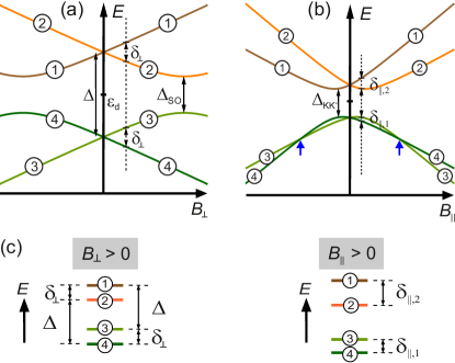
Figure 7: (Color online) Sketch of the evolution of the energy levels in a magnetic field in the case of valley mixing ${\Delta_{\text{KK'}}}$ larger than the spin-orbit coupling ${\Delta_{\text{SO}}}$. (a,b) Single particle spectrum in a magnetic field (a) perpendicular and (b) parallel to the CNT axis. The energy eigenstates are labeled 1-4. At $B=0$ there are two degenerate Kramers pairs separated by $\Delta$. (a) In perpendicular field the energy difference within each chiral pair, i.e., $(1,3)$ and $(2,4)$, remains essentially independent of $B_{\perp}$, provided that $B_{\perp}\lesssim{\Delta_{\text{KK'}}}/g_{\text{s}}\mu_{\text{B}}$. The level splitting within each Kramers doublet is $\delta_{\perp}=g^{\prime}_{s}\mu_{B}B_{\perp}$. An avoided crossing of the particle-hole pair (2,3) occurs when $B_{\perp}\simeq{\Delta_{\text{KK'}}}/g_{\text{s}}\mu_{\text{B}}$. (b) For $B_{\parallel}$ the Aharonov-Bohm effect induces a level crossing of the pair $(3,4)$, as indicated by the blue arrows. (c) Visualization of the level separations from (a) and (b) for values of $B_{\perp}$ and $B_{\parallel}$ corresponding to the dashed lines.

One can easily obtain from Eq. (25) the low and high field asymptotics. The difference $\varepsilon_{1}(B_{\perp})-\varepsilon_{2}(B_{\perp})$ is particularly relevant for our experiments, because at small fields one can extract the effective $g$-factor

$$\begin{split}\delta_{\perp}&=\varepsilon_{1}(B_{\perp})-\varepsilon_{2}(B_{\perp})\simeq g^{\prime}_{\text{s}}\mu_{\text{B}}B_{\perp},\\ g^{\prime}_{\text{s}}&\equiv\frac{g_{\text{s}}}{\sqrt{1+\bigl{(}\Delta_{\text{SO}}/\Delta_{\text{ KK'}}\bigl{)}^{2}}},\end{split}$$ (28)

where $g^{\prime}_{\text{s}}$ is the experimentally measured effective $g$-factor. At large fields, $g_{\text{s}}\mu_{\text{B}}B_{\perp}\gg\sqrt{{\Delta_{\text{KK'}}}^{2}+{\Delta_{\text{SO}}}^{2}}$,

$$\varepsilon_{1}(B_{\perp})-\varepsilon_{2}(B_{\perp})\simeq\Delta_{\text{KK'}}$$ (29)

becomes field independent, providing a direct way to measure $\Delta_{\text{KK'}}$.

A.3 Parallel magnetic field

In the case of the magnetic field oriented along the axis of the carbon nanotube the Hamiltonian takes the form

$$\hat{H}_{\text{CNT}}=\hat{H}^{(0)}_{\text{CNT}}+\hat{H}_{\parallel}(B_{\parallel})=\hat{H}^{(0)}_{\text{CNT}}+g_{\text{orb}}\mu_{\text{B}}B_{\parallel}\hat{I}_{\sigma}\otimes\hat{\tau}_{x}+\\ \frac{1}{2}g_{\text{s}}\mu_{\text{B}}B_{\parallel}\hat{\sigma}_{z}\otimes\hat{I}_{\tau},$$ (30)

where $B_{\parallel}$ is the magnitude of the parallel magnetic field and $g_{\text{orb}}$ is the orbital $g$-factor.

Let us in a similar way address the action of $\hat{\mathcal{T}},\hat{\mathcal{P}}$, and $\hat{\mathcal{C}}$ on the magnetic field dependent part of $\hat{H}_{\text{CNT}}$, i.e., $\hat{H}_{\parallel}(B_{\parallel})=g_{\text{orb}}\mu_{\text{B}}B_{\parallel}\hat{I}_{\sigma}\otimes\hat{\tau}_{x}+\frac{1}{2}g_{\text{s}}\mu_{\text{B}}B_{\parallel}\hat{\sigma}_{z}\otimes\hat{I}_{\tau}$.

A.3.1 Conjugation under time-reversal

In analogy to Eqs. (16), (17) we find

$$\hat{\mathcal{T}}\,\hat{H}_{\parallel}(B_{\parallel})\,\hat{\mathcal{T}}^{-1}=-\hat{H}_{\parallel}(B_{\parallel})=\hat{H}_{\parallel}(-B_{\parallel}),\;\mathrm{or}\\ \{\hat{\mathcal{T}},\hat{H}_{\parallel}(B_{\parallel})\}=0\;,$$ (31)

while the eigenstates $\{|i,B_{\parallel}\rangle,~{}i=1,2,3,4\}$ now obey $\hat{\mathcal{T}}|1,B_{\parallel}\rangle=\kappa|2,-B_{\parallel}\rangle,~{}\hat{\mathcal{T}}|3,B_{\parallel}\rangle=\kappa|4,-B_{\parallel}\rangle$. Correspondingly, the eigenenergies are related through

$$\varepsilon_{1}(B_{\parallel})=\varepsilon_{2}(-B_{\parallel}),\qquad\varepsilon_{3}(B_{\parallel})=\varepsilon_{4}(-B_{\parallel}).$$ (32)

A.3.2 Particle-hole conjugation

If we now look at the action of $\hat{\mathcal{P}}$ we observe

$$\hat{\mathcal{P}}\,\hat{H}_{\parallel}(B_{\parallel})\,\hat{\mathcal{P}}^{-1}=-\hat{H}_{\parallel}(B_{\parallel})=\hat{H}_{\parallel}(-B_{\parallel}),\;\mathrm{or}\\ \{\hat{\mathcal{P}},\hat{H}_{\parallel}(B_{\parallel})\}=0\;,$$ (33)

which implies

$$\begin{split}\hat{\mathcal{P}}(\hat{H}_{\text{CNT}}-\varepsilon_{d}\hat{I}_{\sigma}\otimes\hat{I}_{\tau}-\frac{1}{2}g_{\text{s}}\mu_{\text{B}}B_{\parallel}\hat{\sigma}_{z}\otimes\hat{I}_{\tau})\hat{\mathcal{P}}^{-1}\\ =-(\hat{H}_{\text{CNT}}-\varepsilon_{d}\hat{I}_{\sigma}\otimes\hat{I}_{\tau}-\frac{1}{2}g_{\text{s}}\mu_{\text{B}}B_{\parallel}\hat{\sigma}_{z}\otimes\hat{I}_{\tau}),\quad\\[5.69054pt] \mathrm{or}\quad\{\hat{\mathcal{P}},(\hat{H}_{\text{CNT}}-\varepsilon_{d}\hat{I}_{\sigma}\otimes\hat{I}_{\tau}-\frac{1}{2}g_{\text{s}}\mu_{\text{B}}B_{\parallel}\hat{\sigma}_{z}\otimes\hat{I}_{\tau})\}&=0\;.\end{split}$$ (34)

We see that PH symmetry is still obeyed if we measure the energies with respect to the reference energy $\varepsilon(B_{\parallel})=\varepsilon_{d}+\frac{1}{2}g_{\text{s}}\mu_{\text{B}}B_{\parallel}$, which now depends on $B_{\parallel}$ (cf. Eq. (9)). Furthermore Eq. (10) holds also in parallel magnetic field and hence

$$\begin{split}\varepsilon_{1}(B_{\parallel})-\varepsilon(B_{\parallel})=-\varepsilon_{4}(B_{\parallel})+\varepsilon(B_{\parallel}),\\ \varepsilon_{2}(B_{\parallel})-\varepsilon(-B_{\parallel})=-(\varepsilon_{3}(B_{\parallel})-\varepsilon(-B_{\parallel}))\;.\end{split}$$ (35)

With $\Delta(B_{\parallel})=2(\varepsilon_{1}(B_{\parallel})-\varepsilon(B_{\parallel}))$ one finds:

$$\begin{split}\varepsilon_{1}\left[\varepsilon(B_{\parallel}),\Delta(B_{\parallel})\right]&=\varepsilon_{4}\left[\varepsilon(B_{\parallel}),-\Delta(B_{\parallel})\right],\\ \varepsilon_{2}\left[\varepsilon(-B_{\parallel}),\Delta(-B_{\parallel})\right]&=\varepsilon_{3}\left[\varepsilon(-B_{\parallel}),-\Delta(-B_{\parallel})\right].\end{split}$$ (36)

A.3.3 Chiral conjugation

Regarding chiral conjugation

$$\begin{split}\hat{\mathcal{C}}\,\hat{H}_{\parallel}(B_{\parallel})\,\hat{\mathcal{C}}^{-1}=-\hat{H}_{\parallel}(B_{\parallel})=\hat{H}_{\parallel}(-B_{\parallel}),\;\mathrm{or}\\ [\hat{\mathcal{C}},\hat{H}_{\parallel}(B_{\parallel})]=0\;,\end{split}$$ (37)

we see that $\hat{\mathcal{C}}$ and $\hat{H}_{\parallel}(B_{\parallel})$ commute. Taking into account Eq. (13) it follows that $\hat{\mathcal{C}}$ again does not commute with $\hat{H}_{\text{CNT}}$. The symmetry relations between energies of the $\hat{\cal C}$-conjugated states are analogous to those in Eq. (22). Along similar lines as for the $\hat{\mathcal{P}}$-operation one then finds the relation $\varepsilon_{1}\left[\varepsilon(B_{\parallel}),\Delta_{\parallel}(B_{\parallel})\right]=\varepsilon_{3}\left[\varepsilon(-B_{\parallel}),-\Delta_{\parallel}(-B_{\parallel})\right]$.

The eigenstates $\{|i,B_{\parallel}\rangle,~{}i=1,2,3,4\}$ of the Hamiltonian (30) are easily obtained by taking into account that in parallel field the spin states $\{|\uparrow\rangle,|\downarrow\rangle\}$ are still eigenstates of the total Hamiltonian (30). We find

$$\begin{split}&\begin{bmatrix}|1,B_{\parallel}\rangle\\ |4,B_{\parallel}\rangle\\ |2,B_{\parallel}\rangle\\ |3,B_{\parallel}\rangle\end{bmatrix}=A\begin{bmatrix}|a\uparrow\rangle\\ |b\uparrow\rangle\\ |a\downarrow\rangle\\ |b\downarrow\rangle\end{bmatrix},\quad\mathrm{where}\\[5.69054pt] &A=\begin{bmatrix}\cos\bigl{(}\frac{\Theta^{+}}{2}\bigl{)}&\sin\bigl{(}\frac{\Theta^{+}}{2}\bigl{)}&0&0\\ -\sin\bigl{(}\frac{\Theta^{+}}{2}\bigl{)}&\cos\bigl{(}\frac{\Theta^{+}}{2}\bigl{)}&0&0\\ 0&0&\cos\bigl{(}\frac{\Theta^{-}}{2}\bigl{)}&-\sin\bigl{(}\frac{\Theta^{-}}{2}\bigl{)}\\ 0&0&\sin\bigl{(}\frac{\Theta^{-}}{2}\bigl{)}&\cos\bigl{(}\frac{\Theta^{-}}{2}\bigl{)}\\ \end{bmatrix},\end{split}$$ (38)

and

$$\tan(\Theta^{\pm})=\frac{{\Delta_{\text{SO}}}\pm 2g_{\text{orb}}\mu_{\text{B}}B_{\parallel}}{{\Delta_{\text{KK'}}}}\,.$$ (39)

The corresponding eigenenergies are

$$\boxed{\begin{split}&\varepsilon_{1,4}(B_{\parallel})=\varepsilon(B_{\parallel})\pm\frac{1}{2}\Delta_{\parallel}(B_{\parallel}),\\ &\varepsilon_{2,3}(B_{\parallel})=\varepsilon(-B_{\parallel})\pm\frac{1}{2}\Delta_{\parallel}(-B_{\parallel}),\end{split}}$$ (40)

where $\Delta_{\parallel}(B_{\parallel})=\sqrt{{\Delta_{\text{KK'}}}^{2}+({\Delta_{\text{SO}}}+2g_{\text{orb}}\mu_{\text{B}}B_{\parallel})^{2}}$. Notice the similarity between Eq. (40) and Eq. (25). As in the zero field case, the unitary matrix connecting the two bases, Eq. (38), is block-diagonal in spin space. As in the case of the perpendicular magnetic field, the evolution in the parallel magnetic field represents rotations by angles $\Theta^{\pm}/2$ in two independent two-dimensional planes, $\Theta^{\pm}$-planes, involving the pairs $(1,4)_{P}$ and $(2,3)_{P}$, respectively. The evolution of the energy levels is shown in Fig. 7(b). The relevant energy scales $\varepsilon(B_{\parallel}),\Delta_{\parallel}(B_{\parallel})$ and $\Delta_{\parallel}(-B_{\parallel})$ are illustrated in Fig. 4(b).

As in the case of the perpendicular orientation, one may derive the low and high field asymptotics of Eq. (40). Experimentally relevant quantities at large magnetic fields, $2g_{\text{orb}}\mu_{\text{B}}B_{\parallel}\gg\sqrt{{\Delta_{\text{KK'}}}^{2}+{\Delta_{\text{SO}}}^{2}}$, are the energy differences within a Kramers doublet $\varepsilon_{1}(B_{\parallel})-\varepsilon_{2}(B_{\parallel})$ and $\varepsilon_{3}(B_{\parallel})-\varepsilon_{4}(B_{\parallel})$:

$$\begin{split}&\varepsilon_{1}(B_{\parallel})-\varepsilon_{2}(B_{\parallel})\simeq g_{\text{s}}\mu_{\text{B}}B_{\parallel}+\Delta_{\text{SO}},\\ &\varepsilon_{3}(B_{\parallel})-\varepsilon_{4}(B_{\parallel})\simeq-g_{\text{s}}\mu_{\text{B}}B_{\parallel}+\Delta_{\text{SO}}.\end{split}$$ (41)

Therefore, the relation $[\varepsilon_{1}(B_{\parallel})-\varepsilon_{2}(B_{\parallel})]-[\varepsilon_{4}(B_{\parallel})-\varepsilon_{3}(B_{\parallel})]\simeq 2\Delta_{\text{SO}}$ is valid and provides a direct way to measure the spin-orbit coupling strength $\Delta_{\text{SO}}$. Moreover, the energy difference between chiral pairs is also important. We have

$$\varepsilon_{1}(B_{\parallel})-\varepsilon_{3}(B_{\parallel})\simeq(2g_{\text{orb}}+g_{\text{s}})\mu_{\text{B}}B_{\parallel},$$ (42)

$$\varepsilon_{2}(B_{\parallel})-\varepsilon_{4}(B_{\parallel})\simeq(2g_{\text{orb}}-g_{\text{s}})\mu_{\text{B}}B_{\parallel}.$$ (43)

Thus from the sum $\left[\varepsilon_{1}(B_{\parallel})-\varepsilon_{3}(B_{\parallel})\right]+\left[\varepsilon_{2}(B_{\parallel})-\varepsilon_{4}(B_{\parallel})\right]\simeq 4g_{\text{orb}}\mu_{\text{B}}B_{\parallel}$ the orbital moment can be extracted.

Regarding the low field behavior, we find in leading order in the applied field

$$\begin{split}&\delta_{\parallel,2}=\varepsilon_{1}(B_{\parallel})-\varepsilon_{2}(B_{\parallel})\simeq g^{\prime}_{+}\mu_{\text{B}}B_{\parallel},\\ &\delta_{\parallel,1}=\varepsilon_{3}(B_{\parallel})-\varepsilon_{4}(B_{\parallel})\simeq g^{\prime}_{-}\mu_{\text{B}}B_{\parallel},\\ &g^{\prime}_{\pm}\equiv\frac{2g_{\text{orb}}}{\sqrt{1+\bigl{(}\Delta_{\text{KK'}}/\Delta_{\text{ SO}}\bigl{)}^{2}}}\pm g_{\text{s}},\end{split}$$ (44)

which explicitly shows the difference between the effective $g$-factors of the two Kramers pairs.

A.4 Summary

In Table 1 we compile the (anti-)commutation relations for the different conjugation operations with the different components of $\hat{H}_{\text{CNT}}$, and for $\hat{H}_{\text{CNT}}$ itself.

operation	$\hat{H}^{(0)}_{\text{CNT}}$	$\hat{H}_{\perp}$	$\hat{H}_{\parallel}$	$\hat{H}_{\text{CNT}}$
$\hat{\mathcal{T}}$	commute	anti-comm.	anti-comm.	—
$\hat{\mathcal{P}}$	anti-comm.	anti-comm.	anti-comm.	anti-comm.
$\hat{\mathcal{C}}$	anti-comm.	commute	commute	—

Table 1: (Anti-)commutation rules of the different combinations of operators {$\hat{\mathcal{T}},\hat{\mathcal{P}},\hat{\mathcal{C}}$} and {$\hat{H}^{(0)}_{\text{CNT}},\hat{H}_{\perp},\hat{H}_{\parallel}$} and the resulting (anti-)commutation relations with the total Hamiltonian $\hat{H}_{\text{CNT}}$ in Eq. (2).

The main outcome of our considerations is that both at zero field and for the special cases $B_{\perp},B_{\parallel}$ analyzed in this work the spectrum has to obey the peculiar conjugation relations

$$\boxed{\begin{split}\hat{\mathcal{T}}-\mathrm{conjugation}\,:\\ \;\varepsilon_{1,4}(-\vec{B})=\varepsilon_{2,3}(\vec{B}),\end{split}}$$ (45)

$$\boxed{\begin{split}\hat{\mathcal{P}}-\mathrm{conjugation}\,:\\ \varepsilon_{1}(\vec{B})-\varepsilon(\vec{B})&=\;\varepsilon(\vec{B})-\varepsilon_{4}(\vec{B})={\Delta(\vec{B})}/{2},\\ \varepsilon_{2}(\vec{B})-\varepsilon(-\vec{B})&=\;\varepsilon(-\vec{B})-\varepsilon_{3}(\vec{B})={\Delta(-\vec{B})}/{2},\end{split}}$$ (46)

where $\Delta_{\perp,\parallel}(\vec{B})$ and $\varepsilon(\vec{B})$ depend according to Eqs. (25) and (40) on the modulus and direction of the magnetic field. These conjugation relations are dictated by the effect of the time-reversal operation as well as by a generalized particle-hole operation. All symmetry relations are verified by the diagonalization of $\hat{H}_{\text{CNT}}$. Moreover, it is easy to show using Eq. (2) that Eqs. (45) and (46) hold true also for an arbitrary direction of the magnetic field $\vec{B}$. The conjugation relations impose precise constraints on the form of the Keldysh effective action as we shall discuss below.

Appendix B Many-particle problem and nonequilibrium field theory

The experiments presented address to a large extent the effect of the electron-electron interaction playing an essential role in the behavior of the ultra-clean CNT under investigation. Namely, on top of the nontrivial single-particle spectrum controlled by spin-orbit interaction, valley mixing, and magnetic field, as discussed in the previous section, the strong electronic correlations give rise to a pure many-particle effect, known as the Kondo resonance Hewson (1997), and lead to a new energy scale $k_{\text{B}}T_{\text{K}}$ where $T_{\text{K}}$ is the Kondo temperature. It is this many-particle state which governs the response of the quantum dot to the applied bias voltage $V_{\text{sd}}$. Since in the experiment this voltage can be large, the corresponding energy scale $eV_{\text{sd}}$ can become larger than other energy scales and an appropriate nonequilibrium treatment beyond linear response is required. Therefore, the experiments challenge the theory which must properly take into account the specific single-particle spectrum, in particular, its symmetries, electronic correlations and nonequilibrium. Below we show the basic concepts of our theory which represents an effective field-theoretic approach based on the Keldysh field integral Altland and Simons (2010) capable to comprehensively account for different single-particle spectra, many-particle interactions and nonequilibrium.

B.1 Electron-electron interactions in the quantum dot

Using the states $|i\rangle$, $i=1,2,3,4$, discussed in the previous section the single-particle Hamiltonian, Eq. (2), may be written in the following form

$$\hat{H}_{\text{CNT}}=\sum_{i}\varepsilon_{i}\hat{n}_{i},$$ (47)

where $\hat{n}_{i}=d^{\dagger}_{i}d_{i}$ and $d^{\dagger}_{i}$/$d_{i}$ are the corresponding fermionic creation/annihilation operators. Since the electrons in the quantum dot interact, there is a finite energy cost $U>0$ for two electrons to occupy the same quantum state. The quantum dot Hamiltonian taking into account the effect of interactions is

$$\hat{H}_{\text{d}}=\hat{H}_{\text{CNT}}+\hat{H}_{ee}.$$ (48)

The last term in Eq. (48) describes the electron-electron interactions in the quantum dot. It has the following form:

$$\hat{H}_{ee}=\frac{U}{2}\sum_{i\neq j}\hat{n}_{i}\hat{n}_{j}$$ (49)

and represents one of the key players in the formation of the many-particle Kondo resonance.

Notice that if $\varepsilon_{i}=\varepsilon_{\text{d}}$, $i=1,2,3,4$, the Hamiltonian (48) is invariant under $SU(4)$ transformations,

$$\hat{\mathcal{R}}=\exp\bigl{(}\mathbbmsl{i}\cdot\hat{\mathcal{G}}\bigl{)},$$ (50)

where $\hat{\mathcal{G}}$ is an arbitrary Hermitian traceless operator represented by a four-dimensional matrix in the spin-valley space,

$$\hat{\mathcal{G}}^{\dagger}=\hat{\mathcal{G}},\quad\text{Tr}\bigl{(}\hat{\mathcal{G}}\bigl{)}=0.$$ (51)

In other words, the electron-electron interaction alone cannot break the $SU(4)$ symmetry of the system with ${\Delta_{\text{KK'}}}={\Delta_{\text{SO}}}=0$.

B.2 Tunneling between the quantum dot and contacts

Another essential player responsible for the emergence of the Kondo effect is the tunneling coupling between the quantum dot and the conduction electrons in the contacts. The electrons in the contacts are assumed to be noninteracting. Their Hamiltonian has the form

$$\hat{H}_{\text{C}}=\sum_{xki}\varepsilon_{k}c^{\dagger}_{xki}c_{xki},$$ (52)

where $x$ enumerates the contacts as the left ($x=\text{L}$) and right ($x=\text{R}$) ones, $k$ is the quantum number characterizing the contacts continuum energy spectrum, $\varepsilon_{k}$, assumed to be independent of $i$ and $c^{\dagger}_{xki}$/$c_{xki}$ are the corresponding creation/annihilation operators. The contacts are in equilibrium characterized by chemical potentials $\mu_{\text{L,R}}$ such that $\mu_{\text{R}}-\mu_{\text{L}}=eV_{\text{sd}}$.

The electronic exchange between the quantum dot and the contacts is accounted for through the tunneling Hamiltonian,

$$\hat{H}_{\text{T}}=\sum_{xki}(T_{xk}c^{\dagger}_{xki}d_{i}+T^{*}_{xk}d^{\dagger}_{i}c_{xki}),$$ (53)

where $T_{xk}$ are the tunneling matrix elements. Here we assume that the spin and orbital degrees of freedom labeled via the index $i$ are conserved during the tunneling processes, reflecting the physical situation where the contacts constitute parts of the same CNT and thus might share the same degrees of freedom Choi et al. (2005). The effect of contacts which may mix orbital quantum numbers is thoroughly discussed in Ref. Jespersen et al., 2011. There it is shown that, despite orbital mixing drives the system from the $SU(4)$ Kondo fixed point to the $SU(2)$ Kondo fixed point, still $SU(4)$ Kondo physics governs transport for not too large mixing. Tunneling elements preserving orbital quantum numbers are considered here for simplicity. However, according to Ref. Jespersen et al., 2011, also accounting for a small degree of mixing should not alter the main conclusion of our work.

If $\varepsilon_{i}=\varepsilon_{\text{d}}$, $i=1,2,3,4$, the total Hamiltonian,

$$\hat{H}_{\text{tot}}\equiv\hat{H}_{\text{d}}+\hat{H}_{\text{C}}+\hat{H}_{\text{T}}=\hat{H}_{\text{CNT}}+\hat{H}_{ee}+\hat{H}_{\text{C}}+\hat{H}_{\text{T}},$$ (54)

is still invariant under $SU(4)$ transformations because the tunneling matrix elements are independent of $i$. In this case the model is usually referred to as the $SU(4)$ Anderson model Hewson (1997). Since in our experiments both ${\Delta_{\text{KK'}}}$ and ${\Delta_{\text{SO}}}$ are finite, the $SU(4)$ symmetry is broken.

B.3 Slave-bosonic transformation

The Kondo effect studied in our experiments arises in Coulomb valleys with odd numbers of electrons when the electron-electron interaction $U$ in the quantum dot significantly exceeds the energy $\Gamma$ (see the definition below) characterizing the coupling between the quantum dot and contacts. Therefore, to capture the essence of the Kondo physics it is enough to consider the limit of strong electron-electron interaction, $U\rightarrow\infty$, when the quantum dot can accommodate only one electron. In this case the Hamiltonian (48) can be diagonalized by means of the so-called slave-bosonic transformation Hewson (1997),

$$d_{i}=b^{\dagger}p_{i}\quad d^{\dagger}_{i}=bp^{\dagger}_{i},$$ (55)

where $b^{\dagger}$/$b$ are bosonic, or slave-bosonic, creation/annihilation operators while $p_{i}^{\dagger}$/$p_{i}$ represent new fermionic creation/annihilation operators. Physically Eq. (55) represents a transformation from the electronic states to the states of the quantum dot, empty state ($b^{\dagger}$, $b$) and the state with one electron ($p_{i}^{\dagger}$, $p_{i}$). After the diagonalization $\hat{H}_{\text{d}}$ becomes

$$\hat{H}_{\text{d}}=\sum_{i}\varepsilon_{i}p^{\dagger}_{i}p_{i}.$$ (56)

The contacts Hamiltonian is not affected by this transformation while the tunneling Hamiltonian becomes

$$\hat{H}_{\text{T}}=\sum_{xki}\bigl{(}T_{xk}c^{\dagger}_{xki}b^{\dagger}p_{i}+T^{*}_{xk}bp^{\dagger}_{i}c_{xki}\bigl{)}.$$ (57)

As one can see from Eq. (57), the slave-bosonic transformation simplifying the quantum dot Hamiltonian $\hat{H}_{\text{d}}$ complicates the tunneling Hamiltonian $\hat{H}_{\text{T}}$ which now, instead of products of two second quantized operators, contains products of three second quantized operators. The slave-bosonic and new fermionic operators satisfy the constraint

$$b^{\dagger}b+\sum_{i}p^{\dagger}_{i}p_{i}=\hat{I},$$ (58)

which physically reflects the conservation of the total number of the slave-bosons and new fermions in the quantum dot which can only have zero or one electron.

B.4 Field integral representation for observables

The experimental observable of interest is the differential conductance $G(V_{\text{sd}})=\partial I/\partial V_{\text{sd}}$, which can be obtained by taking the derivative of the current $I$ through the quantum dot with respect to the applied bias voltage $V_{\text{sd}}$. The current through the quantum dot is given by the Meir-Wingreen formula Wingreen and Meir (1994),

$$\begin{split}I&=\frac{e}{\hbar}\sum_{i}\int_{-\infty}^{\infty}\!\!\!\!d\varepsilon[n_{\text{R}}(\varepsilon)-n_{\text{L}}(\varepsilon)]\frac{\Gamma}{4}\frac{W^{2}}{\varepsilon^{2}+W^{2}}\nu_{i}(\varepsilon),\\ n_{\text{L,R}}(\varepsilon)&=\frac{1}{\exp[\beta(\varepsilon-\mu_{0}\pm eV_{\text{sd}}/2)]+1},\end{split}$$ (59)

where $\Gamma\equiv 2\pi\nu_{\text{C}}|\mathfrak{t}|^{2}$ ($\nu_{\text{C}}$ is the contacts density of states, $\mathfrak{t}$ is the value of the tunneling matrix element $T_{xk}$ assumed to be independent of $x$ and $k$), $W$ is the Lorentzian width of the contacts density of states, $\nu_{i}(\varepsilon)$ is the quantum dot tunneling density of states for the state $|i\rangle$, $\beta$ is the inverse temperature and $\mu_{0}$ is the equilibrium chemical potential, $\mu_{\text{L,R}}=\mu_{0}\mp eV_{\text{sd}}/2$.

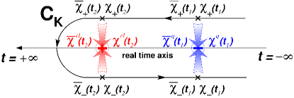
Figure 8: (Color online) The Keldysh contour $C_{\text{K}}$, the basis of our nonequilibrium theory, is shown. It is used to formulate the real time evolution of an interacting nonequilibrium system. Its forward branch goes from $t=-\infty$ to $t=+\infty$, its backward branch from $t=+\infty$ to $t=-\infty$. The slave-bosonic fields $\bar{\chi},\chi$ living on the forward branch are denoted as $\bar{\chi}_{+},\chi_{+}$ while the slave-bosonic fields living on the backward branch are denoted as $\bar{\chi}_{-},\chi_{-}$. The forward and backward branches are mapped onto the real time axis as sums (red arrows at $t_{2}$) or differences (blue arrows at $t_{1}$) turning, respectively, into the classical or quantum slave-bosonic fields via the Keldysh rotation, $\chi^{\text{cl,q}}(t)\equiv(1/\sqrt{2})[\chi_{+}(t)\pm\chi_{-}(t)]$.

Therefore, the problem reduces to the calculation of the quantum dot tunneling density of states,

$$\nu_{j}(\varepsilon)\equiv-\frac{1}{\pi\hbar}\text{Im}[G^{+}_{jj}(\varepsilon)],$$ (60)

where $G^{+}_{jj}(\varepsilon)$ is the quantum dot retarded Green’s function for the eigenstates $|j\rangle$, $j=1,2,3,4$, of the CNT Hamiltonian. To calculate them we develop an effective field theory based on the Keldysh field integral Altland and Simons (2010) where one replaces all the second quantized operators by the corresponding fields. The basic idea of this theory is to use the advantage of the physical clarity provided by the slave-bosonic transformation, introduced in the previous subsection, which allows one to deal directly with the states of the quantum dot. In particular, in the Kondo regime the probability of the empty state of the quantum dot is small and, thus, large fluctuations of the slave-bosonic fields, describing the empty state, are not relevant for the Kondo physics. One can then use a low order expansion in these fields around proper field configurations in order to calculate the quantum dot observables.

The practical implementation of this idea involves a functional integration over all the fermionic, or Grassmann, fields, describing the electrons in contacts and the states of the quantum dot with one electron. After this step one is left with an effective field theory describing the dynamics of the slave-bosonic field. At this stage any quantum dot observable, $\hat{O}=\mathcal{F}(d_{\sigma}^{\dagger}$, $d_{\sigma})$, originally expressed in terms of the second quantized operators, admits a field-theoretic representation based on the Keldysh effective action Smirnov and Grifoni (2011a, b, 2013a):

$$\begin{split}\langle\hat{O}\rangle(t)=\frac{1}{\mathcal{N}_{0}}\underset{\mu\rightarrow\infty}{\text{lim}}e^{\beta\mu}&\int\mathcal{D}[\bar{\chi},\chi]e^{\frac{\mathbbmsl{i}}{\hbar}S_{\text{eff}}[\bar{\chi}^{\text{cl,q}}(\tilde{t});\chi^{\text{cl,q}}(\tilde{t})]}\\ &\times\mathcal{F}[\bar{\chi}^{\text{cl,q}}(t);\chi^{\text{cl,q}}(t)],\\[5.69054pt] S_{\text{eff}}[\bar{\chi}^{\text{cl,q}}(t);\chi^{\text{cl,q}}(t)]=&S_{0}[\bar{\chi}^{\text{cl,q}}(t);\chi^{\text{cl,q}}(t)]\\ &+S_{\text{T}}[\bar{\chi}^{\text{cl,q}}(t);\chi^{\text{cl,q}}(t)],\end{split}$$ (61)

where $\chi^{\text{cl,q}}$ are the classical and quantum Altland and Simons (2010) eigenstates of the bosonic annihilation operator $b$, $\mathcal{N}_{0}$ is a normalization constant Smirnov and Grifoni (2011a) and the limit $\mu\rightarrow\infty$ in Eq. (61) takes into account the constraint in Eq. (58). The Keldysh effective action, $S_{\text{eff}}[\bar{\chi}^{\text{cl,q}}(t);\chi^{\text{cl,q}}(t)]$, in Eq. (61) is the sum of $S_{0}[\bar{\chi}^{\text{cl,q}}(t);\chi^{\text{cl,q}}(t)]$, being the standard free bosonic action Altland and Simons (2010) on the Keldysh contour, Fig. 8, and $S_{\text{T}}[\bar{\chi}^{\text{cl,q}}(t);\chi^{\text{cl,q}}(t)]$, being the tunneling action of the problem.

B.5 Keldysh effective action and tunneling density of states

The tunneling term of the Keldysh effective action,

$$S_{\rm T}[\bar{\chi}^{\rm cl,q}(t);\chi^{\rm cl,q}(t)]=-\mathbbmsl{i}\hbar\,{\rm tr}\ln\bigl{[}-\mathbbmsl{i}G^{(0)-1}-\mathbbmsl{i}\mathcal{T}\bigl{]},$$ (62)

is a highly nonlinear functional of the slave-bosonic fields. Here the matrix $\mathcal{T}$ is off-diagonal in the quantum dot-contacts space,

$$\mathcal{T}=\begin{pmatrix}0&M_{\rm T}^{\dagger}(it|k^{\prime}i^{\prime}t^{\prime})\\ M_{\rm T}(kit|i^{\prime}t^{\prime})&0\end{pmatrix},$$ (63)

$$\begin{split}M_{\rm T}(kit|i^{\prime}t^{\prime})=&\frac{\delta(t-t^{\prime})\delta_{ii^{\prime}}\mathfrak{t}}{\sqrt{2}\hbar}\\ &\times\begin{pmatrix}\bar{\chi}^{\rm cl}(t)-\gamma_{i}\sqrt{2}&\bar{\chi}^{\rm q}(t)\\ \bar{\chi}^{\rm q}(t)&\bar{\chi}^{\rm cl}(t)-\gamma_{i}\sqrt{2}\end{pmatrix},\end{split}$$ (64)

$$\begin{split}M^{\dagger}_{\rm T}(it|k^{\prime}i^{\prime}t^{\prime})=&\frac{\delta(t-t^{\prime})\delta_{ii^{\prime}}\mathfrak{t}^{*}}{\sqrt{2}\hbar}\\ &\times\begin{pmatrix}\chi^{\rm cl}(t)-\delta_{i}\sqrt{2}&\chi^{\rm q}(t)\\ \chi^{\rm q}(t)&\chi^{\rm cl}(t)-\delta_{i}\sqrt{2}\end{pmatrix}.\end{split}$$ (65)

In Eqs. (64) and (65) $\gamma_{i}$ and $\delta_{i}$ ($i=1,2,3,4$) represent the initially arbitrary expansion points or shifts of the classical slave-bosonic fields, $\bar{\chi}^{\text{cl}}$ and $\chi^{\text{cl}}$, respectively, in the slave-bosonic space. As shown below, $\gamma_{i}$ and $\delta_{i}$ can be determined from the symmetries of the Hamiltonian and from the Fermi-liquid behavior at zero temperature and zero bias. Notice, that since the integration variables $\bar{\chi}^{\text{cl,q}}$ and $\chi^{\text{cl,q}}$ are independent of each other, the $\gamma_{i}$ and $\delta_{i}$ are not complex conjugates.

The Green’s function matrix $G^{(0)}$ is block-diagonal in the quantum dot-contacts space. Its quantum dot block $G^{(0)}_{\rm d}$ has the standard $2\times 2$ fermionic Keldysh structure:

$$G^{(0)}_{\rm d}(it|i^{\prime}t^{\prime})=\delta_{ii^{\prime}}\begin{pmatrix}G^{+}_{i}(t-t^{\prime})&G^{\rm K}_{i}(t-t^{\prime})\\ 0&G^{-}_{i}(t-t^{\prime})\end{pmatrix}.$$ (66)

In the frequency domain the components of the above matrix are

$$\begin{split}&G^{+}_{i}(\omega)=\frac{\hbar}{\hbar\omega-(\varepsilon_{i}+\mu)+\mathbbmsl{i}E_{i}},\quad G^{-}_{i}(\omega)=[G^{+}_{i}(\omega)]^{*},\\ &G^{\rm K}_{i}(\omega)=\frac{1}{2}[G^{+}_{i}(\omega)-G^{-}_{i}(\omega)]\sum_{x}\tanh\biggl{[}\frac{\hbar\omega-\mu_{x}}{2k_{\text{B}}T}\biggl{]}.\end{split}$$ (67)

Here $E_{i}\equiv\gamma_{i}\delta_{i}\Gamma/2$.

In the case of the quantum dot tunneling density of states, $\nu_{j}$, for the state $|j\rangle$ the expression for the integrand in Eq. (61) is

$$\begin{split}\mathcal{F}[\bar{\chi}^{\rm cl,q}(t);\chi^{\rm cl,q}(t)]=[\bar{\chi}_{-}(t)\chi_{+}(0)-\bar{\chi}_{+}(t)\chi_{-}(0)]&\times[G^{(0)-1}+\mathcal{T}]^{-1}(jt|j0),\end{split}$$ (68)

where $\bar{\chi}_{\pm}$, $\chi_{\pm}$ are the slave-bosonic fields on the forward and backward branches Altland and Simons (2010) of the Keldysh contour, Fig. 8, and the expansion points, introduced in Eqs. (64) and (65), are labeled by an additional upper index, $\gamma_{i},\delta_{i}\rightarrow\gamma^{j}_{i},\delta^{j}_{i}$ and, as a consequence $E_{i}\rightarrow E^{j}_{i}$.

As mentioned in the previous subsection, to solve this highly nonlinear problem one has to perform an expansion of the tunneling action in powers of the slave-bosonic fields. To get the relevant physics already in the lowest, i.e., in the second order expansion, one must carefully specify the field configurations around which this expansion has to be performed. This can be done with a suitable choice of the expansion points $\gamma^{j}_{i}$ and $\delta^{j}_{i}$. Since the linear terms in the Keldysh effective action do not generate (see Ref. Smirnov and Grifoni, 2013a) any finite contribution to $\nu_{j}(\varepsilon)$, in the second order expansion the expansion points $\gamma^{j}_{i}$ and $\delta^{j}_{i}$ appear only through $E^{j}_{i}$ which determine the form of the propagators in Eq. (67). Therefore, $\gamma^{j}_{i}$ and $\delta^{j}_{i}$ just renormalize the kernel of the quadratic Keldysh effective action.

To properly account for the Kondo correlations specific to CNT quantum dots this renormalization should respect the specific symmetry properties of the energy spectrum. First, since TR symmetry is broken at finite magnetic fields, the Keldysh effective action should also reflect this symmetry breaking together with the $\hat{\mathcal{T}}$-conjugation, Eq. (45). Second, the $\hat{\mathcal{P}}$-conjugation relations, Eq. (46), are valid at any magnetic field and it is natural to construct a Keldysh effective action having these properties as well. It is easy to see that these two requirements lead to a structure of the Keldysh effective action where only two states from different Kramers pairs and from the same particle-hole pair are present in the action.

Finally, to identify which particle-hole pair should be retained in the Keldysh effective action, we recall that the Kondo effect in quantum dots, whose states are characterized by a discrete quantum number $i$, arises from virtual transitions between the electronic states $|i\rangle$ and $|i^{\prime}\rangle$. Even though both flip $i\neq i^{\prime}$ and non flip terms $i=i^{\prime}$ are important for the Kondo resonance, non flip processes alone cannot give rise to the Kondo effect, as seen for example from the analysis of the renormalization group flow equations for the $SU(4)$ Kondo effect in carbon nanotubes Choi et al. (2005). This is similar to the $SU(2)$ Anderson model, where the spin-$1/2$ Kondo behavior arises from the virtual transitions between the electronic states $|\uparrow\rangle$ and $|\downarrow\rangle$ in the quantum dot, which are, in this case, spin flips. Therefore, to properly capture the Kondo behavior already in the lowest order expansion it is natural, in view of the poor man’s scaling where the renormalization flow is governed by flip processes, in the calculation of $\nu_{j}(\varepsilon)$ to effectively eliminate from the kernel of the Keldysh effective action the propagator for the same state $|j\rangle$ (see Eq. (67)).

The above considerations uniquely specify the structure of the Keldysh effective action. To obtain this structure one has to choose the expansion points $\gamma_{i}^{j}$ and $\delta_{i}^{j}$ appropriately. Let us for example discuss how we choose $E^{1}_{i}=\gamma_{i}^{1}\delta_{i}^{1}\Gamma/2$ in the Keldysh effective action for $\nu_{1}(\varepsilon)$. Since the Keldysh effective action for $\nu_{1}(\varepsilon)$ should effectively contain the pair of propagators for the states $|2\rangle$ and $|3\rangle$ only, the expansion points are chosen such that the real and imaginary parts of $E^{1}_{i}$ are

$$\begin{split}E^{1\text{R}}_{1}&=E^{1\text{R}}_{2}=E^{1\text{R}}_{3}=E^{1\text{R}}_{4}=E^{\text{ R}},\\ E^{1\text{I}}_{1}&=E^{\text{I}}-(\varepsilon_{1}-\varepsilon_{2}),\\ E^{1\text{I}}_{2}&=E^{\text{I}},\\ E^{1\text{I}}_{3}&=E^{\text{I}},\\ E^{1\text{I}}_{4}&=E^{\text{I}}-(\varepsilon_{4}-\varepsilon_{3}),\end{split}$$ (69)

where $E^{\text{R,I}}$ are currently arbitrary but their values may be found from the Fermi-liquid behavior (see below). In a similar way the parameters $E^{2}_{i},E^{3}_{i}$, and $E^{4}_{i}$ entering the calculation of $\nu_{2}(\varepsilon),\nu_{3}(\varepsilon)$ and $\nu_{4}(\varepsilon)$, respectively, can be chosen.

Since the Keldysh effective action is quadratic, the final expressions for the tunneling densities of states are obtained by calculating the corresponding Gaussian field integrals. We find

$$\nu_{j}(\varepsilon,\vec{B})=\frac{1}{2\pi}\frac{W^{2}}{\varepsilon^{2}+W^{2}}\frac{\Gamma}{[\varepsilon_{j}(\vec{B})-\varepsilon+\Gamma\Sigma^{\text{R}}_{j}(\varepsilon,\vec{B})]^{2}+[\Gamma\Sigma^{\text{I}}_{j}(\varepsilon,\vec{B})]^{2}}.$$ (70)

In Eq. (70) $\Sigma^{\text{R}}_{j}(\varepsilon,\vec{B})$ and $\Sigma^{\text{I}}_{j}(\varepsilon,\vec{B})$ are, respectively, the real and imaginary parts of the self-energies,

$$\Sigma_{j}(\varepsilon,\vec{B})=-\sum_{i=1}^{4}\frac{1}{2}\int_{-\infty}^{\infty}\frac{d\varepsilon^{\prime}}{2\pi}\frac{W^{2}}{\varepsilon^{\prime 2}+W^{2}}\frac{n_{\text{L}}(\varepsilon^{\prime})+n_{\text{R}}(\varepsilon^{\prime})}{\varepsilon^{\prime}-\varepsilon-(\varepsilon_{i}(\vec{B})-\varepsilon_{j}(\vec{B}))+\mathbbmsl{i}E^{j}_{i}}.$$ (71)

With the $E^{j}_{i}$ chosen as discussed in Eq. (69) this turns into

$$\begin{split}&\Sigma_{1,4}(\varepsilon,\vec{B})=-\sum_{i=2,3}\int_{-\infty}^{\infty}\frac{d\varepsilon^{\prime}}{2\pi}\frac{W^{2}}{\varepsilon^{\prime 2}+W^{2}}\frac{n_{\text{L}}(\varepsilon^{\prime})+n_{\text{R}}(\varepsilon^{\prime})}{\varepsilon^{\prime}-\varepsilon-(\varepsilon_{i}(\vec{B})-\varepsilon_{1,4}(\vec{B}))+\mathbbmsl{i}E},\\ &\Sigma_{2,3}(\varepsilon,\vec{B})=-\sum_{i=1,4}\int_{-\infty}^{\infty}\frac{d\varepsilon^{\prime}}{2\pi}\frac{W^{2}}{\varepsilon^{\prime 2}+W^{2}}\frac{n_{\text{L}}(\varepsilon^{\prime})+n_{\text{R}}(\varepsilon^{\prime})}{\varepsilon^{\prime}-\varepsilon-(\varepsilon_{i}(\vec{B})-\varepsilon_{2,3}(\vec{B}))+\mathbbmsl{i}E},\end{split}$$ (72)

where virtual non flip processes and $\hat{\mathcal{P}}$-processes no longer explicitly appear. It is easy to see from Eq. (72) that, as a result of the time-reversal and particle-hole conjugation relations of the single particle energies $\varepsilon_{j}(\vec{B})$, also the so obtained observables $\nu_{j}(\varepsilon)$ (here we explicitly indicate that $\nu_{j}$ depend on the magnetic field $\vec{B}$ or on the splittings $\Delta(\pm\vec{B})$) fulfill the conjugation relations

$$\nu_{1}(\varepsilon,\vec{B})=\nu_{2}(\varepsilon,-\vec{B}),\quad\nu_{3}(\varepsilon,\vec{B})=\nu_{4}(\varepsilon,-\vec{B}),$$ (73)

$$\begin{split}\nu_{1}(\varepsilon,\Delta(\vec{B}))=\nu_{4}(\varepsilon,-\Delta(\vec{B})),\\ \nu_{2}(\varepsilon,\Delta(-\vec{B}))=\nu_{3}(\varepsilon,-\Delta(-\vec{B})),\end{split}$$ (74)

where $\Delta(\vec{B})\equiv\varepsilon_{1}(\vec{B})-\varepsilon_{4}(\vec{B})$ and $\Delta(-\vec{B})\equiv\varepsilon_{2}(\vec{B})-\varepsilon_{3}(\vec{B})$ according to Eq. (46).

At zero temperature, zero bias and zero magnetic field in Coulomb valleys with odd numbers of electrons the differential conductance reaches its unitary limit value $2e^{2}/h$, as predicted by the Fermi-liquid theory Hewson (1997). The tunneling density of states has a narrow maximum located close to the equilibrium chemical potential $\mu_{0}$. Since in our experiments $\Delta\equiv\sqrt{\Delta^{2}_{\text{KK'}}+\Delta^{2}_{\text{SO}}}\simeq 7k_{\text{B}}T_{\text{K}}$, one can neglect a small deviation from $\mu_{0}$ in the location of this maximum. Using the two conditions, the unitary limit value and location of the maximum, one can obtain the real and imaginary parts $E^{\text{R}}$ and $E^{\text{I}}$. After that the expressions for the tunneling densities of states, Eq. (70), can be used to calculate the differential conductance $G(V_{\text{sd}},T,B)$ as a function of the bias voltage, temperature, and magnetic field.

Note that in principle one might use knowledge of the unitary limit for another observable like the magnetic susceptibility (see Ref. Hewson, 1997), which would not change $E^{\text{R,I}}$ since the unitary limits for different observables are related.

B.6 The Kondo temperature and universality

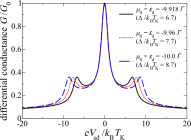
Figure 9: (Color online) The differential conductance as a function of the bias voltage at zero temperature and zero magnetic field for different values of $\mu_{0}-\varepsilon_{d}$ (equivalently for different gate voltages) and for a fixed value of $\Delta$. The Kondo temperature $T_{\text{K}}^{(0)}$ is here rescaled to $T_{\text{K}}$ which is the temperature at which the linear conductance as a function of the temperature is equal to $G_{0}/2$. In our model $G_{0}=2e^{2}/h$, since the couplings to the left and right contacts are assumed to be equal. As one can see, the zero bias peak, or the Kondo peak, is universal while the side peaks are not. The full universality, i.e., the universality at any bias voltage is recovered only if $\Delta/k_{\text{B}}T_{\text{K}}=\text{const}$ which is not the case in our experiments because the gate voltage is altered for a fixed CNT quantum dot, that is for a fixed value of $\Delta$.

The theory presented above predicts the universal behavior of the differential conductance with the scaling given by the Kondo temperature

$$k_{\text{B}}T_{\text{K}}^{(0)}=f\biggl{[}\frac{\Delta}{k_{\text{B}}T_{\text{K}}^{SU(4)}}\biggl{]}2W\exp\biggl{[}-\frac{\mu_{0}-\varepsilon_{d}}{2\Gamma}\biggl{]}$$ (75)

(differing from $k_{\text{B}}T_{\text{K}}$, used in the main text, by a constant prefactor, chosen such that the linear conductance at $T_{\text{K}}$ equals half of its unitary value). In Eq. (75)

$$k_{\text{B}}T_{\text{K}}^{SU(4)}=2W\exp\biggl{[}-\frac{\mu_{0}-\varepsilon_{d}}{2\Gamma}\biggl{]}$$ (76)

is the Kondo temperature for the $SU(4)$ Anderson model and $f(x)$ is a function of the ratio $x=\Delta/k_{\text{B}}T_{\text{K}}^{SU(4)}$. Our theory correctly predicts the limiting behavior of this function. When $\Delta\rightarrow\infty$ ($x\rightarrow\infty$) we find that

$$f(x)\rightarrow\exp\biggl{[}-\frac{\mu_{0}-\varepsilon_{d}}{2\Gamma}\biggl{]}.$$ (77)

This leads to

$$T_{\text{K}}^{(0)}\rightarrow T^{SU(2)}_{\text{K}}=2W\exp\biggl{[}-\frac{\mu_{0}-\varepsilon_{d}}{\Gamma}\biggl{]}.$$ (78)

On the other side, when $\Delta\rightarrow 0$ ($x\rightarrow 0$), we find that

$$f(x)\rightarrow 1$$ (79)

leading to

$$T_{\text{K}}^{(0)}\rightarrow T^{SU(4)}_{\text{K}}.$$ (80)

The correct scaling behavior for any $\Delta$ is one of the advantages of our theory over other theories, e.g., over the equations of motion technique which is a popular tool to investigate the Kondo effect in various setups, in particular, in CNT quantum dots Fang et al. (2008b).

It is essential that the Kondo correlations significantly weaken the loss of universality at energies smaller than $\Delta$. As a result, the central peak remains almost universal: the variation in its width is much smaller than the relative variation (about 30% in Fig. 9) of the Kondo energy scale $k_{\text{B}}T_{\text{K}}$. This behavior is specific to the $SU(4)$ broken Kondo effect and represents its fingerprint when observed in experiments.

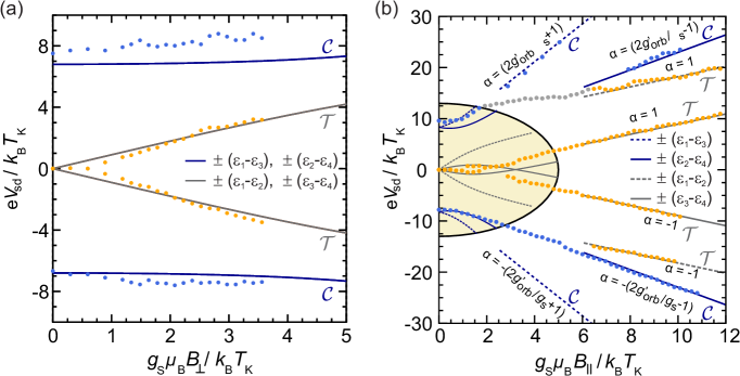
Figure 10: (Color) Calculated single particle energy differences between CNT quantum levels (lines) and corresponding measured positions of conductance peaks (dots) for a wide range of bias voltages and magnetic fields perpendicular (a) and parallel (b) to the CNT axis. In each case, gray lines correspond to intra-Kramers and blue lines to chiral inter-Kramers transitions. For the case of parallel magnetic field (b), a discussion of low field (yellow area) versus high field behaviour can be found in the text. In the high field limit, the $\alpha$-values describe the slopes of the linear magnetic field dependence.

Appendix C Inelastic conductance peaks at high magnetic fields

In this section we discuss in more detail the evolution of the measured conductance peaks in a perpendicular and parallel magnetic field, as shown in Fig. 10 (see also Fig. 6). The evolution of the satellite peak positions with magnetic field is governed by the energy differences $\varepsilon_{1}-\varepsilon_{3}$ and $\varepsilon_{2}-\varepsilon_{4}$ (blue dashed and solid lines). In perpendicular field these differences weakly depend on the magnitude of the magnetic field while they strongly vary in parallel field. Hence, we expect that the location and height of the satellite peaks will not be affected by the perpendicular field $B_{\perp}$ but must strongly depend on $B_{\parallel}$. Indeed, this is what we observe in Fig. 10(a) and Fig. 10(b), respectively. According to our theory, increasing the magnitude of $B_{\parallel}$ shifts the satellite peaks to higher voltages. At $B_{\parallel}\gtrsim 1.1\,k_{\text{B}}T_{\text{K}}/g_{\text{s}}\mu_{\text{B}}$, the satellite peaks split into two peaks (see e.g. the red curve in Fig. 5(f)). By further increasing $B_{\parallel}$, the peak splitting grows while both peaks continue to move to higher voltages. This behavior is again in a good qualitative agreement with our experiments, albeit the second peak splitting occurs at unexpectedly low magnetic field.

In the case of the perpendicular field, Fig. 10(a), the peak positions related to intra-Kramers and chiral inter-Kramers transitions match the expectations from the theory in the whole range of the investigated magnetic field values. On the other hand, in a parallel field one can clearly distinguish between a low field region [contained in the yellow area in Fig. 10(b)] and a high field region. The latter shows a linear dependence both of the peak positions and of the energy differences on the magnetic field. The low field region is defined by the condition $B_{\parallel}\ll\Delta/2g_{\text{orb}}\mu_{\text{B}}$, where $g_{\text{orb}}\mu_{\text{B}}$ is the orbital magnetic moment (see Eq. (2)). With the values of

perpend.	theory	experiment	parallel	theory	experiment
$T_{\text{K}}$ (K)		0.86	$T_{\text{K}}$ (K)		1.12
$\Delta$	6.9	6.8, 7.5	$\Delta$	8.3	7.5, 10
$g_{\text{s}}$	2		$g_{\text{s}}$	2
$g^{\prime}_{\text{s}}$	1.80	$1.85\pm 0.05$	$g_{\text{orb}}/g_{\text{s}}$	2.4
			$g^{\prime}_{\text{orb}}/g_{\text{s}}$	1.37	1.37
$\Delta_{\text{SO}}$	3.0		$\Delta_{\text{SO}}$	3.6	4.7
$\Delta_{\text{KK'}}$	6.2		$\Delta_{\text{KK'}}$	7.5

Table 2: Values of the nanotube parameters as used in the theoretical calculations and extracted from the differential conductance measurements in magnetic fields perpendicular (valley with $N_{\text{el}}=21$) and parallel (valley with $N_{\text{el}}=17$) to the nanotube axis. Energies are given in units of $k_{\text{B}}T_{\text{K}}$. The two values of $\Delta$ given in the experimental columns correspond to the values extracted from the satellite peaks in the differential conductance at negative and positive bias voltages, respectively.

$\Delta/k_{\text{B}}T_{\text{K}}$ and $g_{\text{orb}}$ (see Table 2), used in the numerical calculations, this corresponds to $B_{\parallel}\ll 1.5\,k_{\text{B}}T_{\text{K}}/g_{\text{s}}\mu_{\text{B}}$, where $g_{\text{s}}$ is the spin $g$-factor. In the high field region, $B_{\parallel}\gg\Delta/2g_{\text{orb}}\mu_{\text{B}}$, the valley mixing effects become negligible and the energy eigenstates are products of pure spin and valley states. In this case the data can be fitted to the linearized dispersion relation $\varepsilon_{1,4}(B_{\parallel})\propto\mu_{\text{B}}B_{\parallel}(g_{\text{s}}/2\pm g_{\text{orb}}^{\prime})$ and $\varepsilon_{2,3}(B_{\parallel})\propto\mu_{\text{B}}B_{\parallel}(-g_{\text{s}}/2\pm g_{\text{orb}}^{\prime})$, with $g_{\text{orb}}^{\prime}/g_{\text{s}}=1.37$.

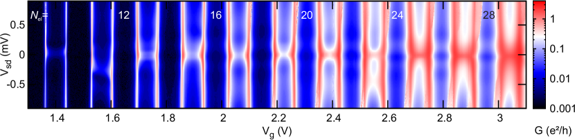
Figure 11: (Color) Differential conductance $G$ as function of bias voltage $V_{\text{sd}}$ and gate voltage $V_{\text{g}}$, for the gate voltage region corresponding to $9\leq N_{\text{el}}\leq 29$.

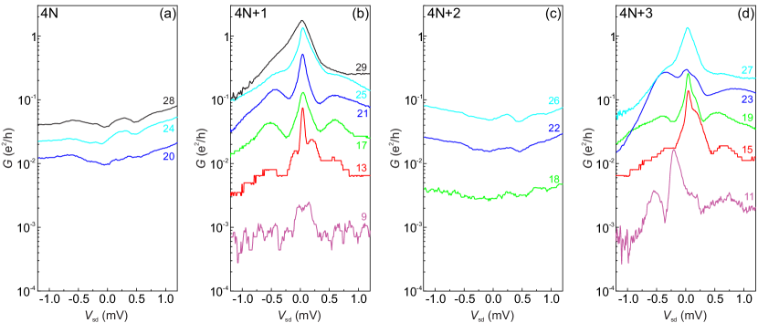
Figure 12: (Color online) Differential conductance $G$ as function of bias voltage $V_{\text{sd}}$, at gate voltages $V_{\text{g}}$ in the center of the Coulomb blockade valleys for differing electron numbers. The four panels each display traces corresponding to a particular residue modulo 4 of the electron number $N_{\text{el}}$.

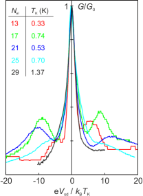
Figure 13: (Color online) Line traces $G(V_{\text{sd}})$ from Fig. 12(b), i.e., at the center of Coulomb blockade valleys with occupation $4N+1$, with $V_{\text{sd}}$ rescaled by the corresponding Kondo temperature $T_{\text{K}}$ and the conductance rescaled by its maximum value $G_{0}=G(V_{\text{sd}}=0)$.

This amounts to a ratio between high field and low field orbital g-factors of $g_{\text{orb}}^{\prime}/g_{\text{orb}}=0.57$. Notice that such asymptotic behavior is also predicted by expanding the spectrum of the effective Hamiltonian $\hat{H}_{\text{CNT}}$ at large fields, see Eqs. (41), (44), but there $g_{\text{orb}}^{\prime}/g_{\text{orb}}=1$. This suggests the presence of a mechanism which reduces the ratio of the orbital $g$-factors that is not captured by the Hamiltonian $\hat{H}_{\text{CNT}}$ and goes beyond the scope of this work. This is the reason why only a qualitative but not quantitative agreement between theory and experiment in the investigated range of applied parallel fields is found. Accounting for this discrepancy, it is possible to identify all Kondo transitions observed in the experiment as either intra-Kramers or chiral inter-Kramers transitions. In particular intra-Kramers transitions involving the excited Kramers doublet $(1,2)_{T}$ become visible at larger fields (see dashed gray line in Fig. 10(b)), while they are not discernible at small magnitudes of the parallel magnetic field.

Finally, in the linear regime $B_{\perp}\gtrsim 5.3\,B_{c}$ it is possible to experimentally extract the effective $g$-factor $g^{\prime}_{\text{s}}=g_{\text{s}}/\sqrt{1+({\Delta_{\text{SO}}}/{\Delta_{\text{KK'}}})^{2}}$ (see Eq. (28)), and hence to directly access the ratio ${\Delta_{\text{SO}}}/{\Delta_{\text{KK'}}}$ for the valley $N_{\text{el}}=21$. Similarly, from the linear regime $B_{\parallel}\gtrsim 1.75\,B_{\text{c3}}$ we can directly extract $\Delta_{\text{SO}}$ (see Eq. (41)) for the valley $N_{\text{el}}=17$. These values together with the parameters used in the numerical calculations are shown in Table 2.

Appendix D Systematic evolution of the transport spectrum with the electron number

To demonstrate the generic character of the observed fine structure of the Kondo resonance in charging states with odd electron number, we present a more comprehensive overview over the different Coulomb valleys for electron numbers between 9 and 29.

Fig. 11 displays the stability diagram measurement, i.e. the differential conductance $G$ as function of bias voltage $V_{\text{sd}}$ and gate voltage $V_{\text{g}}$, of this parameter region. Because of the onset of mechanical self-excitation of the suspended nanotube Steele et al. (2009); Schmid et al. (2012) (as e.g. already visible left to the electron number labels “24” and “28” in the figure) the measurement was restricted to comparatively low bias voltages. Satellite maxima accompanying the zero-bias Kondo anomaly at odd electron number can be recognized for a wide range of $N_{\text{el}}$.

In Fig. 12 conductance traces $G(V_{\text{sd}})$ taken at gate voltages corresponding to the center of a Coulomb blockade region are sorted by the filling state of shells corresponding to different longitudinal modes. In the odd valleys the distinct zero-bias peak can be observed. Additionally, satellite peaks systematically occur in all odd valleys with an overall increase of the Kondo temperature with increasing electron number. The universal behavior of the central peak and the non-universal behavior of the satellites is further illustrated also by Fig. 13, where the conductance traces of Fig. 12(b) have been rescaled with the corresponding Kondo temperatures, similar to main text Fig. 1(d). In the even valleys $N_{\text{el}}=4N,N_{\text{el}}=4N+2$ the traces are nearly flat with weak features around zero bias whose origin is unclear. They gradually vanish with increasing magnetic field.

It is evident that the level structure of our CNT sample is highly regular in terms of shell filling, allowing us to describe the fine structure of the Kondo resonances in different valleys by solely slightly adjusting the internal parameters $\Delta_{\text{SO}}$ and $\Delta_{\text{KK'}}$. We conclude that the fine structure of the Kondo effect occurs systematically in all valleys with odd electron numbers between 11 and 27.

References

- Kondo (1964) J. Kondo, Prog. Theo. Phys. 32, 37 (1964).
- Goldhaber-Gordon et al. (1998a) D. Goldhaber-Gordon et al., Nature 391, 156 (1998a).
- Goldhaber-Gordon et al. (1998b) D. Goldhaber-Gordon et al., Phys. Rev. Lett. 81, 5225 (1998b).
- Cronenwett et al. (1998) S. M. Cronenwett, T. H. Oosterkamp, and L. P. Kouwenhoven, Science 281, 540 (1998).
- Grobis et al. (2008) M. Grobis, I. G. Rau, R. M. Potok, H. Shtrikman, and D. Goldhaber-Gordon, Phys. Rev. Lett. 100, 246601 (2008).
- Gaass et al. (2011) M. Gaass, A. K. Hüttel, K. Kang, I. Weymann, J. von Delft, and C. Strunk, Phys. Rev. Lett. 107, 176808 (2011).
- Cao et al. (2005) J. Cao, Q. Wang, and H. Dai, Nature Mat. 4, 745 (2005).
- Nygård et al. (2000) J. Nygård, H. C. Cobden, and P. E. Lindelof, Nature 408, 342 (2000).
- Jarillo-Herrero et al. (2005) P. Jarillo-Herrero, J. Kong, H. S. J. van der Zant, C. Dekker, L. P. Kouwenhoven, and S. De Franceschi, Nature 434, 484 (2005).
- Makarovski et al. (2007) A. Makarovski, A. Zhukov, J. Liu, and G. Finkelstein, Phys. Rev. B 75, 241407 (2007).
- Borda et al. (2003) L. Borda, G. Zaránd, W. Hofstetter, B. I. Halperin, and J. von Delft, Phys. Rev. Lett. 90, 026602 (2003).
- Choi et al. (2005) M.-S. Choi, R. López, and R. Aguado, Phys. Rev. Lett. 95, 067204 (2005).
- Lim et al. (2006) J. S. Lim, M.-S. Choi, M. Y. Choi, R. López, and R. Aguado, Phys. Rev. B 74, 205119 (2006).
- Fang et al. (2008a) T.-F. Fang, W. Zuo, and H.-G. Luo, Phys. Rev. Lett. 101, 246805 (2008a).
- Fang et al. (2010) T.-F. Fang, W. Zuo, and H.-G. Luo, Phys. Rev. Lett. 104, 169902 (2010).
- Lim et al. (2011) J. S. Lim, R. López, G. L. Giorgi, and D. Sánchez, Phys. Rev. B 83, 155325 (2011).
- Galpin et al. (2010) M. R. Galpin, F. W. Jayatilaka, D. E. Logan, and F. B. Anders, Phys. Rev. B 81, 075437 (2010).
- Kuemmeth et al. (2008) F. Kuemmeth, S. Ilani, D. C. Ralph, and P. L. McEuen, Nature 452, 448 (2008).
- Del Valle et al. (2011) M. Del Valle, M. Margańska, and M. Grifoni, Phys. Rev. B 84, 165427 (2011).
- Steele et al. (2013) G. A. Steele, F. Pei, E. A. Laird, J. M. Jol, H. B. Meerwaldt, and L. P. Kouwenhoven, Nature Comm. 4, 1573 (2013).
- Ando (2000) T. Ando, J. Phys. Soc. Jpn. 69, 1757 (2000).
- Jespersen et al. (2011) T. S. Jespersen, K. Grove-Rasmussen, J. Paaske, K. Muraki, T. Fujisawa, J. Nygård, and K. Flensberg, Nature Physics 7, 348 (2011).
- Grove-Rasmussen et al. (2012) K. Grove-Rasmussen, S. Grap, J. Paaske, K. Flensberg, S. Andergassen, V. Meden, H. I. Jørgensen, K. Muraki, and T. Fujisawa, Phys. Rev. Lett. 108, 176802 (2012).
- Marganska et al. (2014) M. Marganska, P. Chudzinski, and M. Grifoni, (2014), arXiv:1412.7484 .
- Garnier et al. (1997) M. Garnier, K. Breuer, D. Purdie, M. Hengsberger, Y. Baer, and B. Delley, Phys. Rev. Lett. 78, 4127 (1997).
- Reinert et al. (2001) F. Reinert, D. Ehm, S. Schmidt, G. Nicolay, S. Hüfner, J. Kroha, O. Trovarelli, and C. Geibel, Phys. Rev. Lett. 87, 106401 (2001).
- Ernst et al. (2011) S. Ernst, S. Kirchner, C. Krellner, C. Geibel, G. Zwicknagl, F. Steglich, and S. Wirth, Nature 474, 362 (2011).
- Quay et al. (2007) C. Quay, J. Cumings, S. Gamble, R. de Picciotto, H. Kataura, and D. Goldhaber-Gordon, Phys. Rev. B 76, 245311 (2007).
- Lan et al. (2012) Y.-W. Lan, K. Aravind, C.-S. Wu, C.-H. Kuan, K.-S. Chang-Liao, and C.-D. Chen, Carbon 50, 3748 (2012).
- Cleuziou et al. (2013) J. P. Cleuziou, N. V. N’Guyen, S. Florens, and W. Wernsdorfer, Phys. Rev. Lett. 111, 136803 (2013).
- Kong et al. (1998) J. Kong, H. T. Soh, A. M. Cassell, C. F. Quate, and H. Dai, Nature 395, 878 (1998).
- Liang et al. (2001) W. Liang, M. Bockrath, D. Bozovic, J. H. Hafner, M. Tinkham, and H. Park, Nature 411, 665 (2001).
- Wegewijs and Nazarov (2001) M. R. Wegewijs and Y. V. Nazarov, arXiv:cond-mat/0103579v2 (2001).
- Paaske et al. (2006) J. Paaske, A. Rosch, P. Wölfle, N. Mason, C. M. Marcus, and J. Nygård, Nature Physics 2, 460 (2006).
- Note (1) The precise expression for the Kondo temperature is extracted from the many-body theory calculations, yielding . Experimentally, fluctuations of between different measurement runs were observed, leading to corresponding fluctuations of the obtained values. For consistency we use throughout the evaluation of the center of valley .
- Kretinin et al. (2012) A. V. Kretinin, H. Shtrikman, and D. Mahalu, Phys. Rev. B 85, 201301(R) (2012).
- Pletyukhov and Schoeller (2012) M. Pletyukhov and H. Schoeller, Phys. Rev. Lett. 108, 260601 (2012).
- Yamada et al. (1984) K. Yamada, K. Yosida, and K. Hanzawa, Prog. Theo. Phys. 71, 450 (1984).
- Schrieffer and Wolff (1966) J. Schrieffer and P. Wolff, Phys. Rev. 149, 491 (1966).
- Altland and Simons (2010) A. Altland and B. Simons, Condensed Matter Field Theory, 2nd ed. (Cambridge University Press, Cambridge, 2010).
- Smirnov and Grifoni (2013a) S. Smirnov and M. Grifoni, Phys. Rev. B 87, 121302(R) (2013a).
- Smirnov and Grifoni (2013b) S. Smirnov and M. Grifoni, New J. Phys. 15, 073047 (2013b).
- Laird et al. (2014) E. A. Laird, F. Kuemmeth, G. Steele, K. Grove-Rasmussen, J. Nygård, K. Flensberg, and L. P. Kouwenhoven, (2014), arXiv:1403.6113 .
- Altland and Zirnbauer (1997) A. Altland and M. R. Zirnbauer, Phys. Rev. B 55, 1142 (1997).
- (45) The term particle-hole symmetry refers here to the fact that the corresponding operator exchanges states at energies located symmetrically around a reference energy ( or ) within the quadruplet. It must not be confused with the particle-hole symmetry around the band gap.
- (46) The asymmetry of the peaks in the experiment is attributed to the difference in the coupling strength to the left and right contacts; for simplicity, in the theoretical curves the coupling to the left and right contacts is assumed to be of the same strength.
- Note (2) For the theoretical calculations in Figs. 6(a) and 6(c) we use the same independently determined parameters as in Fig. 5. To fit the high field data in Fig. 6(b) a smaller orbital -factor than at low field was used (see Table 2).
- Wingreen and Meir (1994) N. S. Wingreen and Y. Meir, Phys. Rev. B 49, 11040 (1994).
- (49) Notice that the expansion point are in general function of temperature and bias. It turns out, however, that is sufficient to fix their value from conditions on the TDOS at zero temperature and bias. In fact for this choice of parameters the expansion points are of the order of the Kondo temperature, and hence do not play a role at high energies. However, their finite value is crucial in the Fermi liquid regime reached at low energies.
- Huertas-Hernando et al. (2006) D. Huertas-Hernando, F. Guinea, and A. Brataas, Phys. Rev. B 74, 155426 (2006).
- Izumida et al. (2009) W. Izumida, K. Sato, and R. Saito, J. Phys. Soc. Jpn. 78, 074707 (2009).
- Hewson (1997) A. C. Hewson, The Kondo Problem to Heavy Fermions (Cambridge University Press, 1997).
- Smirnov and Grifoni (2011a) S. Smirnov and M. Grifoni, Phys. Rev. B 84, 125303 (2011a).
- Smirnov and Grifoni (2011b) S. Smirnov and M. Grifoni, Phys. Rev. B 84, 235314 (2011b).
- Fang et al. (2008b) T.-F. Fang, W. Zuo, and H.-G. Luo, Phys. Rev. Lett. 101, 246805 (2008b).
- Steele et al. (2009) G. A. Steele, A. K. Hüttel, B. Witkamp, M. Poot, H. B. Meerwaldt, L. P. Kouwenhoven, and H. S. J. van der Zant, Science 325, 1103 (2009).
- Schmid et al. (2012) D. R. Schmid, P. L. Stiller, C. Strunk, and A. K. Hüttel, New Journal of Physics 14, 083024 (2012).