Quantum Origins Of Objectivity

Abstract

In spite of all of its successes, quantum mechanics leaves us with a central problem: How does Nature create a ”foot-bridge” from fragile quanta to the objective world of everyday experience? Here we find that a basic structure within quantum mechanics that leads to the perceived objectivity is a, so called, spectrum broadcast structure. We uncover this basing on minimal assumptions, without referring to any dynamical details or a concrete model. More specifically, working formally within the decoherence theory setting with multiple environments (known as quantum Darwinism), we show how a crucial for quantum mechanics notion of non-disturbance due to Bohr and a natural definition of objectivity lead to a canonical structure of a quantum system-environment state, reflecting objective information records about the system stored in the environment.

I Introduction

The emergence of objective world from quanta has been a long standing problem, already present from the very dawn of quantum mechanics old_bohr ; old_heis ; modern . One of the most promising approaches is the decoherence theory, based on a system-environment paradigm Zeh ; Schloss : a quantum system is considered interacting with its environment. It recovers, under certain conditions, a classical-like behavior of the system alone in some preferred frame, singled out by the interaction and called a pointer basis ZurekPRD , and explains it through information leakage from the system into the environment. However, decoherence theory is silent on how comes that in the classical realm information is redundant ZurekNature : same record can exist in a large number of copies and can be independently accessed by many observers and many times. Or more basically: Since quanta cannot be cloned no_cloning and information redundancy is—from the observers’ measurements perspective—at the heart of objectivity, then what quantum process lies at the foundations of the objective classical world ?

Recently, a crucial step was made in a series of works (see e.g. ZurekNature ; ZwolakZurek ) introducing quantum Darwinism idea. Its essence is that in more realistic environments, composed of many independent fractions, decoherence leads to an appearance of multiple copies of system’s state in the environment, accessible to independent observers. Although presenting a convincing physical picture, there is no general, model-independent justification of such claims apart from studies under the strict conditions of specific models, e.g. spin-$1/2$ systems Zurek_spins or an illuminated sphere sfera_zurek . However, even those studies still do not present totally convincing arguments within the models themselves, as they are based on a scalar information-theoretical condition and, so called, "partial information plots", which are known to be only a necessary condition for objectivity but its sufficiency is still unknown.

Here we take a more fundamental and rigorous position, based solely on what as for now provides the most basic description of Nature: A quantum state (see also generic ). More precisely, we derive from first principles a universal, objectivity-carrying structure of quantum states, using a general approach, independent of any dynamics (much like e.g. the S-matrix theory in the quantum field theory Cao ): Looking at the post-interaction system-environments state, we ask what properties should it have to reflect the objectivity. Surprisingly, the answer comes with a help of Bohr’s notion of non-disturbance Bohr ; Wiseman , which originally used to defend the quantum EPR ; Bohr , here, ironically, defines the classical. It is obtained through, what we call, a spectrum broadcast structure, which precisely pin-points the distributed character of information and makes it essentially classical. We finally illustrate our approach on one of the emblematic examples of the decoherence theory: A dielectric sphere illuminated by photons sfera ; sfera_zurek ; myPRL . It must be mentioned that in the quantum Darwinism literature there appeared similar quantum state structures (so called "branching states"). However, they have been at best tacitly postulated ZurekNature ; ZwolakZurek ; ZurekPRA06 , if at all explicitly mentioned. Our results allow to understand an intimate connection between the perceived objectivity, a specific structure of quantum states, and information broadcasting.

II General Theorem

II.1 Basic Definitions And The Main Result

We first define the central concepts of our study and state the main result. The basis of our work is the following definition of an objective state ZurekNature ; Ollivier :

Definition 1 (Objectivity)

A state of the system $S$ exists objectively if many observers can find out the state of $S$ independently, and without perturbing it.

As it stands, the above definition is rather informal and has to be made more rigorous. For example the key concept of perturbation has to be made precise. We do it in the next Subsection.

Second key concept of our study is a spectrum broadcast structure, defined below.

Definition 2 (Spectrum Broadcast Structure)

Spectrum broadcast structure is the following form of a joint state of the central system $S$ and a collection of sub-environments $E_{1},\dots,E_{fN}$ (denoted by $fE$):

$$\varrho_{S:fE}=\sum_{i}p_{i}|i\rangle_{S}\langle i|\otimes\varrho^{E_{1}}_{i}\otimes\cdots\otimes\varrho^{E_{fN}}_{i},$$ (1)

where $\{|i\rangle\}$ is some basis in the system’s space, $p_{i}$ are probabilities, and all states $\varrho^{E_{k}}_{i}$ are perfectly distinguishable:

$$\varrho^{E_{k}}_{i}\varrho^{E_{k}}_{i^{\prime}}=0\ \text{ for all}\ i\neq i^{\prime}\text{ and for all }k=1,\dots,fN.$$ (2)

All the nomenclature will be clarified in the next Subsection. This is a special form of, so called, classical-classical states, which have been introduced as a counterpart of separable states in the context of quantification of quantum correlations Oppenheim ; CC . It has first appeared in a context of quantum channels in my .

The main result of this work is establishing of an intimate connection between these two concepts. The two pivotal assumptions we will use are that of Bohr non-disturbance Bohr ; Wiseman and strong independence. The first has been formulated in Wiseman (see Section II.2), while by the strong independence we mean that the only correlation between the environments should be the common information about the system. In other words, conditioned by the information about the system, there should be no correlations between the environments. This is in a sense an idealization, which we use since we are interested in the information flow only between the system and each of the environments, but not between the environments themselves. Under these central assumptions (together with some auxiliary ones), we prove in Section II.3 the following Theorem:

Theorem 1

Assume that a system undergoes a full decoherence. Then the appearance of a spectrum broadcast structure is a necessary and sufficient condition for objectivity in the sense of Definition 1:

$$\begin{array}[]{c}\text{Objective Existence}\bm{\Leftarrow}\text{Spectrum Broadcast Structure}\\ \left(\begin{array}[]{c}\text{Objective}\\ \text{Existence}\end{array}\right)+\left(\begin{array}[]{c}\text{Strong}\\ \text{Independence}\end{array}\right)\bm{\Rightarrow}\left(\begin{array}[]{c}\text{Spectrum}\\ \text{Broadcast}\\ \text{Structure}\end{array}\right).\end{array}$$ (10)

II.2 Formalization of Definition 1

Here we put Definition 1 into a physical frame and make it as precise as possible, which is the hardest work. As the most suitable, we formally choose decoherence theory with multiple environments ZurekNature : The quantum system of interest $S$ interacts with multiple environments $E_{1},\dots,E_{N}$ (denoted collectively as $E$), also modeled as quantum systems. The environments (or their collections) are assumed to be macroscopic and are monitored by independent observers ZwolakZurek . The motivation behind such a choice is that in real-life situations there is always present some interaction with the environment (unless very special conditions are met) and we, the observers, have usually access only to a small portion of it, each to a different. However, as we will see in what follows, no assumptions on the dynamics will be needed. In fact, we may forget about the dynamics altogether and pose a more general question: which multipartite system-environment states reflect objectively existing state of the system in the sense of Def. 1?

We only assume that the system-environment interaction is such that it leads to a full decoherence. The standard, or even paradigmatic, case corresponding to the latter is a physical situation when there exists a time scale $\tau_{D}$, called the decoherence time, such that asymptotically for interaction times $t\gg\tau_{D}$: i) there emerges in the system’s Hilbert space a unique, stable in time pointer basis $\{|i\rangle\}$; ii) the reduced state of the system $\varrho_{S}$ becomes stable and diagonal in the pointer basis:

$$\varrho_{S}\equiv{\rm Tr}_{E}\varrho_{S:E}\approx\sum_{i}p_{i}|i\rangle\langle i|,$$ (11)

where $p_{i}$’s are some probabilities and by $\approx$ we will always denote asymptotic equality in the deep decoherence limit $t/\tau_{D}\to\infty$. However, it should be stressed, that while we usually will mean the latter situation, our derivation of the structure of objectivity, covers also possible situations when the process happens in finite time. We assume here the above explained full decoherence, so that the system decoheres in a basis rather than in higher-dimensional pointer superselection sectors. This is, because we want to consider the full objectivisation of a given quantum degree of freedom, rather than a partial one. Clearly, the environment must be of a large dimension to have a big informational capacity, needed to carry highly redundant records about the decohered system $S$. Moreover, some loss of information is needed (and of course in fact happens in the reality), as otherwise there will be no decoherence, and we assume that some of the environments pass unobserved. The observed environments $E_{1},\dots,E_{fN}$ we denote by $fE$ (depending on the context).

Next, we specify the observers. Apart from the environmental ones, we also allow for a (possibly hypothetical) direct observer, who can measure the system $S$ directly. Such an observer is needed as a reference, to verify that the findings of the environmental observers are the same as if one had a direct access to the system.

The word ”find out” we translate as the observers performing von Neumann—as perfectly repeatable contrary to the generalized—measurements on their subsystems. It should be stressed here that von Neumann measurement, with its repeatability property, has been chosen since we identify the spectrum broadcast structure as the paradigmatic, ideal structure of the state, responsible for objectivity. Indeed, this is the the object to which any real physical state should be compared with, if we want to know, whether the objectivity in more or less approximate sense (in terms of a state trace distance) takes place. (Note that it can be compared with the ideal singlet as the target state of quantum distillation or the ideal channel, in the case of coding theory, to which the outputs of real protocols or physical situations are compared).

By the ”independence” requirement of Def. 1, there can be no correlations between them. Consequently, the global von Neumann measurement, resulting from the individual local observers’ measurements, must be fully product:

$$\Pi^{M_{S}}_{i}\otimes\Pi^{M_{1}}_{j_{1}}\otimes\cdots\otimes\Pi^{M_{fN}}_{j_{fN}},$$ (12)

where $M_{S},M_{1},\dots,M_{fN}$ denote measurements on $S,E_{1},\dots,E_{fN}$ respectively and all $\Pi$’s are mutually orthogonal Hermitian projectors, $\Pi^{M_{k}}_{j}\Pi^{M_{k}}_{j^{\prime}\neq j}=0$. The observers so determine the probabilities $p_{i}$ of $|i\rangle$ in (11) (they must know the pointer basis $\{|i\rangle\}$, as if not, they would not know what information they get is all about). As explained before Theorem 1, we will actually demand more by assuming the strong independence.

The most crucial clarification needed in Definition 1 is to make precise the word "perturbing". We apply here Bohr’s notion of non-disturbance Bohr ; Wiseman , according to which given local measurements on the subsytems are non-disturbing if they leave the whole joint state invariant (after forgetting the results). This is a realistic mathematical idealization of a repetitive information extraction—a crucial prerequisite for objectivity.

We recall that Bohr’s non-distrurbance was formulated in order to save the completeness of quantum theory against the famous Einstein-Podolsky-Rosen argument EPR . Bohr argued Bohr that the EPR notion of mechanical non-disturbance (which amounts to the no-signaling principle Wiseman ) was too restricted and a broader notion was needed. Hence, accepting the completeness of quantum theory, as we do for the purpose of this work, one is forced to accept Bohr’s notion of non-disturbance.

Finally, the independent measurements will typically reveal inconsistent information about the system (see however generic ). Indeed, allowing for general correlations may lead to a disagreement: if one of the observers measures first, the ones measuring afterwards may find outcomes depending on the result of the first measurement. Thus, we add to Def. 1 an obvious agreement requirement: ”…many observers can find out the same state of $S$ independently…”.

II.3 Proof of Theorem 1

We are now ready for a proof of Theorem 1 with the additional assumption of strong independence, explained in Section II.1. We first prove that spectrum broadcast structure from Definition 2 is a sufficient condition for an objectively existing state of the system, in the sense of Definition 1. Indeed, from (1) projections on $|i\rangle$ and on the disjoint supports of $\varrho^{E_{k}}_{i}$ constitute the non-demolition measurements. Performing them independently, all the observers will repeatedly detect the same index $i$ with probabilities $\{p_{i}\}$, without Bohr-disturbing the joint $S:fE$ state, thus making the sate $|i\rangle$ exist objectively in a sense of Def. 1 (cf. ZurekPRA ).

We now prove in the opposite direction. We assume the decoherence has taken place (cf. generic ). Crucial here is the Bohr’s non-disturbance condition from Subsection II.2. Together with the product structure (12), it implies that on each subsystem $S,E_{1},...E_{fN}$ there exists a non-demolition von Neumann measurement, leaving the whole asymptotic state $\varrho_{S:fE}(\infty)$ of the system and the observed environment invariant (the symbol $\infty$ stands here either for the $t/\tau_{D}\to\infty$ asymptotic, or as mentioned before, for any time scale, may be finite, after which the objectivity structure emerges). For $S$ it is defined by the projectors on $|i\rangle$. For the environments we allow for higher-rank projectors $\Pi^{M_{k}}_{j}$,$k=1,...,fN$, not necessarily spanning the whole space, as the environments can have inner degrees of freedom not correlating to $S$.

Consequently, the total joint probability of the results of the Bohr non-disturbing measurements is given by :

$$p_{ij_{1}\dots j_{fN}}\equiv{\rm Tr}\left[|i\rangle\langle i|\otimes\Pi^{M_{1}}_{j_{1}}\otimes\cdots\otimes\Pi^{M_{fN}}_{j_{fN}}\varrho_{S:fE}(\infty)\right].$$ (13)

Now the agreement requirement from Subsection II.2 leads to a natural conclusion:

$$p_{ij_{1}\dots j_{fN}}\neq 0\ \text{ iff }\ i=j_{1}=...=j_{fN}.$$ (14)

Let us more formally show it, considering for simplicity only two observers. If one of them measures first and gets a result $i$, then the joint conditional state becomes $\varrho_{|i}=(1/p_{i})(\Pi_{i}\otimes{\bf 1})\varrho(\Pi_{i}\otimes{\bf 1})$, $p_{i}\equiv{\rm Tr}(\Pi_{i}\otimes{\bf 1}\varrho)$ and the subsequent measurement by the second observer will yield results $j$ with conditional probabilities $p_{j|i}=(1/p_{i}){\rm Tr}(\Pi_{i}\otimes\Pi_{j}\varrho)$. If for some $i$, $p_{j|i}p_{j^{\prime}|i}\neq 0$ for $j\neq j^{\prime}$, then comparing their results after a series of measurements at some later moment, the observers will be confused as to what exactly the state the system $S$ was: with the probability $p_{j|i}p_{j^{\prime}|i}$ the second observer will obtain different states $j\neq j^{\prime}$, while the first observer measured the same state $i$. One would not have the observers’ findings objective, unless for every $i$ there exists only one $j(i)$ such that $p_{j(i)|i}\neq 0$ (actually $p_{j(i)|i}=1$, which follows from the normalization $\sum_{i}p_{i|j}=1$, so that the distributions $p_{\cdot|i}$ are all deterministic). Reversing the measurement order and applying the same reasoning, we obtain that for every $j$ there can exist only one $i(j)$ such that $\tilde{p}_{i(j)|j}\neq 0$, where by the Bayes theorem $\tilde{p}_{i|j}=p_{j|i}p_{i}/\tilde{p}_{j}$, $\tilde{p}_{j}\equiv{\rm Tr}({\bf 1}\otimes\Pi_{j}\varrho)$. These two conditions imply that the joint probability $p_{ij}=p_{i}\delta_{ij}$ (after an eventual renumbering). Applying the above argument to all the pairs of indices, one obtains (14). This means that the environmental Bohr-nondisturbing measurements must be perfectly correlated with the pointer basis.

Hence, after forgetting the results, the asymptotic, post-measurement state $\varrho^{M}_{S:fE}(\infty)$ reads:

$$\varrho^{M}_{S:fE}(\infty)\equiv\sum_{i,j_{1},\dots,j_{fN}}p_{ij_{1}\dots j_{fN}}\varrho_{ij_{1}\dots j_{fN}}^{S:fE}(\infty)$$

$$=\sum_{i}|i\rangle\langle i|\otimes{\bf\Pi}_{i}\,\varrho_{S:fE}(\infty)\,|i\rangle\langle i|\otimes{\bf\Pi}_{i},$$ (15)

where ${\bf\Pi}_{i}\equiv\Pi^{M_{1}}_{i}\otimes\cdots\otimes\Pi^{M_{fN}}_{i}$.

Now we are ready for the key step: we impose the relevant form of the Bohr-nondisturbance condition:

$$\sum_{i}|i\rangle\langle i|\otimes{\bf\Pi}_{i}\,\varrho_{S:fE}(\infty)\,|i\rangle\langle i|\otimes{\bf\Pi}_{i}=\varrho_{S:fE}(\infty),$$ (16)

whose only solution Wiseman are Classical-Quantum (CQ) states QC :

$$\varrho_{S:fE}(\infty)=\sum_{i}p_{i}|i\rangle\langle i|\otimes{\bf R}^{fE}_{i},$$ (17)

where $p_{i}$ are identified with the probabilities from Eq. (11) and ${\bf R}_{i}^{fE}$ are some residual states in the space of the observed environments with mutually orthogonal supports: ${\bf R}_{i}^{fE}{\bf R}_{i^{\prime}\neq i}^{fE}=0$. Hence, ${\bf R}^{fE}_{i}$ are perfectly distinguishable through the assumed non-disturbing measurements ${\bf\Pi}_{i}$, projecting on their supports.

Finally, let us look at the residual states ${\bf R}_{i}^{fE}$ in (17). The demand of the independent ability to determine the state of $S$, already used in (12), completed with the strong independence condition (cf. Section II) leads to the following: Once one of the observers finds a particular result $i$, the resulting conditional state should be fully product. Since the direct observer is already uncorrelated by (17), this implies that:

$${\bf R}_{i}^{fE}=\varrho^{E_{1}}_{i}\otimes\cdots\otimes\varrho^{E_{fN}}_{i}.$$ (18)

and $\varrho^{E_{k}}_{i}$ must be perfectly distinguishable for each $E_{k}$, cf. (2), since by (16) for any $k$ it holds: $\Pi^{M_{k}}_{i}\varrho^{E_{k}}_{i}\Pi^{M_{k}}_{i}=\varrho^{E_{k}}_{i}$ and $\Pi^{M_{k}}_{i}\Pi^{M_{k}}_{i^{\prime}\neq i}=0$. This finishes the proof.

Some remarks are in order. First, in the course of the proof we have formulated a broader class of independent environments, in a way paradigmatic in quantum information theory 0way : the environments are independent if and only if the environmental observers may produce the states (18,2), exploting only local operations (equivalent to local trace preserving maps), i.e. independent environments are those ones that simulate strong independence from the perspective of a specific resource (the class of local operations).

Second, the meaning of the Theorem 1 is that it provides an ideal reference structure for objectivity—the broadcast structure (1). Any other non-ideal situation should be compared to that broadcast structure no matter what figure of merit is taken. On the level of the states, this must be the trace norm which has the clear probabilistic interpretation, where the degree of objectivity is just the trace norm distance to the broadcast state. The transition:

$$\text{\emph{initial $S:E$ state}}\longrightarrow\text{\emph{spectrum broadcast structure (\ref{br2})}}$$

identifies a basic process, called here state information broadcasting, responsible for an appearance of the perceived objectivity. Formally, it involves broadcasting of a part of information about the system—the spectrum of its state after the decoherence, $\text{Sp}\varrho_{S}\equiv\{p_{i}\}$, into the environments and is thus similar to quantum state broadcasting and spectrum my broadcasting. Condition (2) forces the correlations in (1) to be entirely classical and thus the detailed structures of $\varrho^{E_{k}}_{i}$ become irrelevant for the correlations. From (1) and (2) it follows that under a suitable convergence:

$$I\left[\varrho_{S:fE}(\infty)\right]=H_{S}\ \text{ for every fraction }f,$$ (19)

where $I(\varrho_{AB})\equiv S_{\text{vN}}(\varrho_{A})+S_{\text{vN}}(\varrho_{B})-S_{\text{vN}}(\varrho_{AB})$ is the quantum mutual information, $S_{\text{vN}}(\varrho)\equiv-{\rm Tr}(\varrho\log\varrho)$ stands for the von Neumann entropy, and $H_{S}\equiv S_{\text{vN}}[\varrho_{S}(\infty)]=H(\{p_{i}\})$ is the entropy of the decohered state (11). Condition (19), postulated as a sufficient condition for objectivity in quantum Darwinism model, has a clear meaning in the classical information theory ThomasCover : every fraction $f$ carries the same information $H_{S}$ about the system—the latter is redundantly encoded in the environment. However, in the quantum world its sense remains unclear (see the next Section). Here, (19) follows automatically from the deeper structure (1).

III Discussion Of The Entropic Objectivity Condition As A "Witness" For Objectivity

Here we show a potential problem with the entropic objectivity condition (19). as a sufficient condition for objectivity (see e.g. Refs. ZurekNature ; ZwolakZurek and references therein). Although our example below is not fully conclusive, we argue that at this moment neither is the reasoning of quantum Darwinism studies.

Condition (19) has been shown to hold in several models, including the illuminated sphere sfera_zurek ; myPRL and spin baths Zurek_spins . For finite times $t$, the equality (19) is not strict and holds within some error $\delta(t)$, which defines the redundancy $R_{\delta}(t)$ as the inverse of the smallest fraction of the environment $f_{\delta(t)}$, for which $I[\varrho_{S:f_{\delta(t)}E}(t)]=[1-\delta(t)]H_{S}$. When satisfied, (19) implies that the mutual information between the system and the environment fraction is a constant function of the fraction size $f$ (up to an error $\delta$ for finite times) and the plot of $I$ against $f$ exhibits a characteristic plateau, called the classical plateau (see e.g. Ref. ZurekNature ). The appearance of this plateau has been heuristically explained in the quantum Darwinism literature as a consequence of the redundancy: classical information about the system exists in many copies in the environment fractions and can be accessed independently and without perturbing the system by many observers, thus leading to objective existence of a state of $S$ ZurekNature . That would be for sure so in the classical information setting: the condition (19) is there equivalent to a perfect correlation of both systems ThomasCover , i.e. for every $f$ the environment fraction has a full information about the system and indeed this information thus exists objectively in the sense of our definition.

But in the quantum world the situation may be different and the condition (19) alone may not be sufficient to guarantee objectivity, due to a wholistic nature of quantum correlations Michal . It is clear that the spectrum broadcast states (1) satisfy (19), but there may also be entangled states satisfying it, thus violating the spectrum broadcast form, derived as a necessary condition for objectivity. As a simple example in favour of such a statement consider the following state of two qubits, where one is the system $S$ and the second the environment $E$:

$$\varrho_{S:E}\equiv pP_{\left(a|00\rangle+b|11\rangle\right)}+(1-p)P_{\left(a|01\rangle+b|10\rangle\right)},$$ (20)

where $P_{\psi}\equiv|\psi\rangle\langle\psi|$, $p\neq 1/2$, $a=\sqrt{p}$ and $b=\sqrt{1-p}$. Then the partial state $\varrho_{S}=\tilde{p}|0\rangle\langle 0|+(1-\tilde{p})|1\rangle\langle 1|$, $\tilde{p}\equiv pa^{2}+(1-p)b^{2}$ is diagonal in the basis $|0\rangle,|1\rangle$ and moreover $S_{\text{vN}}(\varrho_{S})=S_{\text{vN}}(\varrho_{S:E})\equiv h(\tilde{p})$ (the binary Shannon entropy ThomasCover ), so that a form of the entropic condition holds: $I(\varrho_{S:E})=S_{\text{vN}}(\varrho_{S})=H_{S}$, $H_{S}=h(\tilde{p})$, but the systems are nevertheless entangled, which one verifies directly through the PPT criterion PPT .

The above example is of course not conclusive, as there is only one environment, but it suggest that the functional condition (19) in principle might indeed be not sufficient to show objectivity, as defined in the main text. We leave this, in general uneasy, question open for further sesearch. In the above context it can be already seen what is the paradigmatic shift with respect to the earlier works on decoherence and quantum Darwinism models we propose here: it is the pivotal observation govering our approach that the core object of the analysis should be a derived structure of the full quantum state of the system $S$ and the observed environment $fE$, rather than the partial state of the system only (Decoherence Theory) or information-theoretical functions (quantum Darwinism).

IV Spectrum Broadcast Structure In The Illuminated Sphere Model

We exemplify the general findings from Section II on one of the central models of decoherence (see e.g. sfera ; sfera_zurek ; myPRL ): a dielectric sphere illuminated by photons (for the details see Appendix A). We show that in the course of the evolution a broadcast state (1) is asymptotically formed in this model, assuming for simplicity pure environments (see myPRL for a more general analysis). The sphere is initially in a state without a well defined position (e.g. in $|\psi^{S}_{0}\rangle=(|\vec{x}_{1}\rangle+|\vec{x}_{2}\rangle)/\sqrt{2}$). Photons scatter elastically and slightly differently depending on where the sphere is, but this difference is vanishingly small for each individual scattering: If the observed fraction is too small, the post scattering states $|\Psi^{mic}_{i}\rangle\equiv{\bf S}_{i}|\vec{k}_{0}\rangle$ (${\bf S}_{i}$ are the scattering matrices) become identical in the thermodynamic limit: $\langle\Psi^{mic}_{2}|\Psi^{mic}_{1}\rangle\equiv\langle\vec{k}_{0}|{\bf S}_{2}^{\dagger}{\bf S}_{1}\vec{k}_{0}\rangle\xrightarrow{\text{therm.}}1$ and the joint post scattering state approaches effectively a product: $(\sum_{i=1,2}p_{i}|\vec{x}_{i}\rangle\langle\vec{x}_{i}|)\otimes|\Psi^{mic}\rangle\langle\Psi^{mic}|^{\otimes\mu}$, where probabilities $p_{i}\equiv|\langle\psi_{0}^{S}|\vec{x}_{i}\rangle|^{2}$ form the spectrum of the decohered state (cf. (11)). The photons thus force the sphere to be in a definite position $\vec{x}_{i}$ with the probability $p_{i}$, but the observed fraction carries no information about it (a product phase; see Appendix A.3).

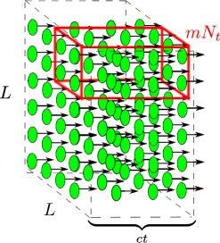
Figure 1: (Color online) Coarse-graining of the photonic environment. The photons (green) scattered in time $t$ are grouped into $M$ equal macroscopic fractions $mN_{t}$. Only one fraction (bounded by the red cage) is shown; $L$ is the edge of an artificial box used for quantization (and removed later; see Appendix A). The macro-fractions may be thought of as representing a sensitivity of the photon detectors (e.g. an eye) and their exact size, $mN_{t}$, is irrelevant–scaling with the total photon number $N_{t}$ suffices.

However, when grouped into macroscopic fractions, the photons become almost perfectly resolving. Imagine we divide all the photons scattered up to time $t$, $N_{t}$, into $M$ macro-fractions of $mN_{t}$, $0<m<1$, photons, Fig. 1. Then the macroscopic post scattering states $|\Psi^{mac}_{i}(t)\rangle\equiv({\bf S}_{i}|\vec{k}_{0}\rangle)^{\otimes mN_{t}}$, become asymptotically perfectly distinguishable:

$$\left|\langle\Psi_{2}^{mac}(t)|\Psi_{1}^{mac}(t)\rangle\right|\xrightarrow{\text{therm.}}\text{e}^{-\frac{m}{\tau_{D}}t},$$ (21)

where $\tau_{D}$ is the decoherence time sfera ; sfera_zurek . If we observe $fM$, $0<f<1$, macro-fractions out of $M$, then the joint post scattering state has asymptotically the spectrum broadcast structure (1):

$$\varrho_{S:fE}(0)=\varrho^{S}_{0}\otimes\underbrace{\varrho_{0}^{mac}\otimes\dots\otimes\varrho^{mac}_{0}}_{fM}\xrightarrow[\text{therm.}]{t\gg\tau_{D}}\varrho_{S:fE}(\infty)=$$

$$\sum_{i=1,2}p_{i}|\vec{x}_{i}\rangle\langle\vec{x}_{i}|\otimes\underbrace{|i^{mac}\rangle\langle i^{mac}|\otimes\dots\otimes|i^{mac}\rangle\langle i^{mac}|}_{fM},$$ (22)

where $|i^{mac}\rangle\equiv|\Psi_{i}^{mac}(\infty)\rangle$ emerges, due to (21), as the non-disturbing environmental basis in the space of each macro-fraction. Eq. (22) identifies the state information broadcasting process: the information about the sphere’s localization, $\{p_{i}\}$, is redundantly transfered into the environment and becomes available in multiple copies through the measurements in $\{|i^{mac}\rangle\}$. The process consists of: i) decoherence sfera and ii) orthogonalization (21), and defines a broadcasting phase, see Appendix A.3, corresponding to the classical plateau of sfera_zurek . From Fannes-Audenaert FAd and Alicki-Fannes FannesAlicki inequalities, the entropic condition (19) follows as a consequence of (22) (see Appendix A.4). Finally, if all the photons are observed, the post-scattering state maintains the full quantum correlation with the system and $I[\varrho_{S:fE}(\infty)]=I_{max}$ (a full information phase).

V Discussion

In conclusion, based on an universal approach, independent of any dynamics or a concrete model, we have identified the primitive state information broadcasting process responsible for an emergence of the perceived objectivity (for a possible loosening of some of our assumptions see generic ). Our main result (Thm. 1) suggests that the states of the form (22) are notoriously formed in Nature. In a laboratory, this can be in principle directly verified via e.g. quantum state tomography tomo . Moreover, it naturally leads to a view that in fact there may be no "quantum-to-classical transition"—what we perceive as "classical", e.g. objective information, may be merely a reflection of some specific properties of the underlying quantum states, like the spectrum broadcast structure; a view further strengthened by ont .

There appears to be a deep connection between the non-signaling principle and objective existence in the sense of Definition 1: the core fact that it is at all possible for observers to determine independently the classical state of the system is guaranteed by the non-signaling principle: ${\rm Tr}({\bf 1}_{S}\otimes\Pi_{E}\varrho_{S:E})={\rm Tr}_{E}(\Pi_{E}\varrho_{E})$. There is no contradiction with the Bohr-nondisturbance, as the latter is a strictly stronger condition than the non-signaling Wiseman (this is the core of Bohr’s reply Bohr to EPR). In fact, the above connection reaches deeper than quantum mechanics. In a general theory, where it is possible to speak of probabilities $p(ij|MN)$ of obtaining results $i,j$ when performing measurements $M,N$ (however defined), whatever the definition of objective existence may be, the requirement of the independent ability to locally determine probabilities by each party seem indispensable. This is guaranteed in the non-signaling theories, where all $p(ij|MN)$’s have well defined marginals. In this sense non-signaling seems a prerequisite of cognition. In this context, we also believe that our approach to objectivity will open a new perspective on the celebrated Bell Theorem Bell . These connections will be the subject of a further research.

The emergence of redundantly encoded information in the structure of quantum states may also shed new light on the life phenomenon. Since self-replication of the DNA information is indispensable for the existence of life, it cannot be excluded that the state information broadcasting may indeed open a ”classical window” for life processes within quantum mechanics Wigner .

Acknowledgements We thank W. H. Zurek and C. J. Riedel for discussions and comments and M. Piani for discussions on strong independence. P.H. and R.H. acknowledge discussions with K. Horodecki, M. Horodecki, and K. Życzkowski. This research is supported by ERC Advanced Grant QOLAPS and National Science Centre project Maestro DEC-2011/02/A/ST2/00305.

Appendix A Technical Details The Illuminated Sphere Model For Pure Environments

A.1 Description of the model

Here we present a detailed derivation of the spectrum broadcast structure (1) in the illuminated sphere model for pure environments (cf. myPRL for a more general situation). We first recall the basics of the model, following the usual treatment (see e.g. Refs. sfera ; GallisFleming ; sfera_zurek ; RiedelZurek ). The system $S$ is a sphere of radius $a$ and relative permittivity $\epsilon$, bombarded by a constant flux of photons, which constitute the multiple environments and decohere the sphere. The sphere can be located only at two positions: $\vec{x}_{1}$ or $\vec{x}_{2}$, so that effectively its state-space is that of a qubit ${\cal H}_{S}\equiv\mathbb{C}^{2}$ with a preferred orthonormal (due to the mutual exclusiveness) basis $|\vec{x}_{1}\rangle$, $|\vec{x}_{2}\rangle$, which will become the pointer basis. This greatly simplifies the analysis, yet allows the essence of the effect to be observed. The sphere is sufficiently massive, compared to the energy of the radiation, so that the recoil due to the scattering can be totally neglected and photons’ energy is conserved, i.e. the scattering is elastic.

The environmental photons are assumed not energetic enough to individually resolve the sphere’s displacement $\Delta x\equiv|\vec{x}_{2}-\vec{x}_{1}|$:

$$k\Delta x\ll 1,$$ (23)

where $\hbar k$ is the characteristic photon momentum. Otherwise, each individual photon would be able to resolve the position of the sphere and studying multiple environments would not bring anything new. On the technical side, following the traditional approach sfera ; GallisFleming ; sfera_zurek ; RiedelZurek , we describe the photons in a simplified way using box normalization: we assume that the sphere and the photons are enclosed in a large box of edge $L$ and volume $V=L^{3}$ and photon momentum eigenstates $|\vec{k}\rangle$ obey periodic boundary conditions. Although a more rigorous treatment was developed in Ref. HornbergerSipe with well localized photon states, we choose this traditional heuristic approach as, at the expense of a mathematical rigor, it allows to expose the physical situation more clearly, without unnecessary mathematical details (we remark that the findings of Ref. HornbergerSipe agree with the previous works using box normalization Adler ). After dealing with formally divergent terms, we remove the box through the thermodynamic limit (signified by $\cong$) sfera_zurek ; RiedelZurek :

$$V\to\infty,N\to\infty,\frac{N}{V}=\text{const},$$ (24)

that is we expand the box and add more photons, keeping the photon density constant, as the relevant physical quantity is the radiative power, proportional to $N/V$. The thermodynamic limit is crucial in the sense that it defines micro- and macroscopic regimes, which will turn to be qualitatively very distinct.

The detailed dynamics of each individual scattering is irrelevant—the individual scatterings are treated asymptotically in time. The interaction time $t$ enters the model differently, thought the number of scattered photons. It may be called a ”macroscopic time”. Assuming photons come from the area of $L^{2}$ at a constant rate $N$ photons per volume $V$ per unit time, the amount of scattered photons from $t=0$ to $t$ is:

$$N_{t}\equiv L^{2}\frac{N}{V}ct,$$ (25)

where $c$ is the speed of light. Throughout the calculations we work with a fixed time $t$ and pass to the asymptotic limit $t/\tau_{D}\to\infty$ (signified by $\approx$ or $\infty$) at the very end.

Since multiphoton scatterings can be neglected and all the photons are treated equally (symmetric environments), the effective sphere-photons interaction up to time $t$ is of a controlled-unitary form:

$$U_{S:E}(t)\equiv\sum_{i=1,2}|\vec{x}_{i}\rangle\langle\vec{x}_{i}|\otimes\underbrace{{\bf S}_{i}\otimes\dots\otimes{\bf S}_{i}}_{N_{t}},$$ (26)

where (assuming translational invariance of the photon scattering) ${\bf S}_{i}\equiv{\bf S}_{\vec{x}_{i}}=e^{-i\vec{x}_{i}\cdot\vec{\hat{k}}}{\bf S}_{0}e^{i\vec{x}_{i}\cdot\vec{\hat{k}}}$ is the scattering matrix when the sphere is at $\vec{x}_{i}$, ${\bf S}_{0}$ is the scattering matrix when the sphere is at the origin, and $\hbar\vec{\hat{k}}$ is the photon momentum operator. Due to the elastic scattering, ${\bf S}_{i}$’s have non-zero matrix elements only between the states $|\vec{k}\rangle$ of the same energy $\hbar c|\vec{k}|$. In the sector (23) the interaction (26) is vanishingly small at the level of each individual photon RiedelZurek : in the thermodynamic limit ${\bf S}_{1}\cong{\bf S}_{2}$ (in a suitable sense we clarify later), and hence $\sum_{i}|\vec{x}_{i}\rangle\langle\vec{x}_{i}|\otimes{\bf S}_{i}\cong{\bf 1}\otimes{\bf S}$. Surprisingly, this will not be true for macroscopic groups of photons. We also note that unlike in the previous treatments sfera ; GallisFleming ; sfera_zurek ; RiedelZurek ; HornbergerSipe , already at this moment we explicitly include in the description all the photons scattered up to the fixed time $t$. Finally, the preferred role of the basis $|\vec{x}_{i}\rangle$ is already singled out now by the form of the interaction (26) ZurekNature .

The initial, pre-scattering ”in” state, is as usually assumed a full product:

$$\varrho_{S:E}(0)\equiv\varrho^{S}_{0}\otimes(\varrho^{ph}_{0})^{\otimes N_{t}},$$ (27)

with $\varrho^{S}_{0}$ having coherences in the preferred basis $|\vec{x}_{i}\rangle$ and $\varrho^{ph}_{0}$ some initial states of the photons (the environments are by assumption symmetric). Next, we introduce a crucial environment coarse-graining ZurekNature : the full environment (i.e. all the $N_{t}$ photons) is divided into a number of macroscopic fractions, each containing $mN_{t}$ photons, $0\leq m\leq 1$. By macroscopic we will always understand ”scaling with the total number of photons $N_{t}$”. By definition, these are the environment fractions accessible to the independent observers. Such a division may seem artificial and arbitrary, as e.g. the choice of $m$ is unspecified. However, observe that in typical situations detectors used to monitor fractions of the environment, e.g. eyes, have some minimum detection thresholds—some minimum amount of radiative energy delivered in a given time interval is needed to trigger the detection. Each macroscopic fraction $mN_{t}$ is meant to reflect that detection threshold. Its concrete value (the fraction size $m$) is for our analysis irrelevant—it is enough that it scales with $N_{t}$. This coarse-graining procedure is analogous to the one used e.g. in the description of liquids: each point of a liquid (a macro-fraction $m$ here) is in reality composed of a suitable large number of microparticles (individual photons). It is also employed in mathematical approach to von Neumann measurements using, so called, macroscopic observables (see e.g. Ref. Sewell and the references therein).

Thus, we divide the detailed initial state of the environment $(\varrho^{ph}_{0})^{\otimes N_{t}}$ into $M\equiv 1/m$ macroscopic fractions:

$$\underbrace{\varrho^{ph}_{0}\otimes\dots\otimes\varrho^{ph}_{0}}_{N_{t}} = \underbrace{\varrho^{ph}_{0}\otimes\dots\otimes\varrho^{ph}_{0}}_{mN_{t}}\otimes\dots\otimes\underbrace{\varrho^{ph}_{0}\otimes\dots\otimes\varrho^{ph}_{0}}_{mN_{t}}$$ (28)

$$\equiv \underbrace{\varrho_{0}^{mac}\otimes\dots\otimes\varrho^{mac}_{0}}_{M},$$

where $\varrho_{0}^{mac}\equiv(\varrho^{ph}_{0})^{\otimes mN_{t}}$ is the initial state of each macroscopic fraction (macro-state for brevity).

A.2 Dynamical formation of broadcast structure

After all the $N_{t}$ photons have scattered, the asymptotic (in the sense of the scattering theory) ”out”-state $\varrho_{S:E}(t)\equiv U_{S:E}(t)\varrho_{S:E}(0)U_{S:E}(t)^{\dagger}$, is given from Eqs. (26,27,28) by

$$\varrho_{S:E}(t)=$$

$$\sum_{i=1,2}\langle\vec{x}_{i}|\varrho^{S}_{0}\,\vec{x}_{i}\rangle|\vec{x}_{i}\rangle\langle\vec{x}_{i}|\otimes\underbrace{\varrho_{i}^{mac}(t)\otimes\dots\otimes\varrho_{i}^{mac}(t)}_{M}$$ (29)

$$+\sum_{i\neq j}\langle\vec{x}_{i}|\varrho^{S}_{0}\,\vec{x}_{j}\rangle|\vec{x}_{i}\rangle\langle\vec{x}_{j}|\otimes\underbrace{\left({\bf S}_{i}\varrho^{ph}_{0}{\bf S}_{j}^{\dagger}\right)^{\otimes mN_{t}}\otimes\dots}_{M}$$ (30)

where

$$\varrho_{i}^{mac}(t)\equiv\left({\bf S}_{i}\varrho^{ph}_{0}{\bf S}_{i}^{\dagger}\right)^{\otimes mN_{t}},\,i=1,2.$$ (31)

In order for the decoherence to take place, some of the environment must be traced out. In the current model it is important that the forgotten fraction must be macroscopic: we assume that $fM$, $0\leq f\leq 1$ out of all $M$ macro-fractions of Eq. (28) are observed, while the rest, $(1-f)M$, is traced out. The resulting partial state reads (cf. Eqs. (29,30)):

$$\varrho_{S:fE}(t)=\sum_{i=1,2}\langle\vec{x}_{i}|\varrho^{S}_{0}\,\vec{x}_{i}\rangle|\vec{x}_{i}\rangle\langle\vec{x}_{i}|\otimes\left[\varrho_{i}^{mac}(t)\right]^{\otimes fM}$$ (32)

$$+\sum_{i\neq j}\langle\vec{x}_{i}|\varrho^{S}_{0}\,\vec{x}_{j}\rangle\left({\rm Tr}{\bf S}_{i}\varrho^{ph}_{0}{\bf S}_{j}^{\dagger}\right)^{(1-f)N_{t}}|\vec{x}_{i}\rangle\langle\vec{x}_{j}|\otimes$$

$$\qquad\qquad\qquad\qquad\qquad\qquad\otimes\left({\bf S}_{i}\varrho^{ph}_{0}{\bf S}_{j}^{\dagger}\right)^{\otimes fN_{t}}.$$ (33)

We finally demonstrate that in the soft scattering sector (23), the above state is asymptotically of the broadcast form (1) by showing that in the deep decoherence regime $t\gg\tau_{D}$ two effects take place:

1. The coherent part $\varrho_{S:fE}^{i\neq j}(t)$ given by Eq. (33) vanishes in the trace norm:

   $$||\varrho_{S:fE}^{i\neq j}(t)||_{\text{tr}}\equiv{\rm Tr}\sqrt{\left[\varrho_{S:fE}^{i\neq j}(t)\right]^{\dagger}\varrho_{S:fE}^{i\neq j}(t)}\approx 0.$$ (34)

2. The post-scattering macroscopic states $\varrho_{i}^{mac}(t)$ (cf. Eq. (31)) become perfectly distinguishable:

   $$\varrho_{1}^{mac}(t)\varrho_{2}^{mac}(t)\approx 0,$$ (35)

   or equivalently using the generalized overlap Fuchs :

   $$B\left[\varrho^{mac}_{1}(t),\varrho^{mac}_{2}(t)\right]\equiv$$

   $$\quad\quad\quad\equiv{\rm Tr}\sqrt{\sqrt{\varrho^{mac}_{1}(t)}\varrho^{mac}_{2}(t)\sqrt{\varrho^{mac}_{1}(t)}}\approx 0,$$ (36)

   despite of the individual (microsopic) states becoming equal in the thermodynamic limit.

The first mechanism above is the usual decoherence of $S$ by $fE$—the suppression of coherences in the preferred basis $|\vec{x}_{i}\rangle$. Some form of quantum correlations may still survive it, since the resulting state (32) is generally of a Classical-Quantum (CQ) form QC . Those relict forms of quantum correlations are damped by the second mechanism: the asymptotic perfect distinguishability (35) of the post-scattering macro-states $\varrho_{i}^{mac}(t)$. Thus, the state $\varrho_{S:fE}(\infty)$ becomes of the spectrum broadcast form (1) for the distribution:

$$p_{i}=\langle\vec{x}_{i}|\varrho^{S}_{0}\,\vec{x}_{i}\rangle.$$ (37)

We demonstrate the mechanisms (34,35), and hence a formation of the broadcast state (1), for pure initial environments:

$$\varrho_{ph}^{0}\equiv|\vec{k}_{0}\rangle\langle\vec{k}_{0}|,\ k_{0}\Delta x\ll 1,$$ (38)

i.e. all the photons come from the same direction and have the same momenta $\hbar k_{0}$, $k_{0}\equiv|\vec{k}_{0}|$, satisfying (23). To show (34), observe that $\varrho_{S:fE}^{i\neq j}(t)$, defined by Eq. (33), is of a simple form in the basis $|\vec{x}_{i}\rangle$:

$$\varrho_{S:fE}^{i\neq j}(t)=\left[\begin{array}[]{cc}0&\gamma C\\ \gamma^{*}C^{\dagger}&0\end{array}\right],$$ (39)

where $\gamma\equiv\langle\vec{x}_{1}|\varrho^{S}_{0}\,\vec{x}_{2}\rangle({\rm Tr}{\bf S}_{1}\varrho^{ph}_{0}{\bf S}_{2}^{\dagger})^{(1-f)N_{t}}$ and $C\equiv({\bf S}_{1}\varrho^{ph}_{0}{\bf S}_{2}^{\dagger})^{\otimes fN_{t}}$. Since ${\bf S}_{i}$’s are unitary and $\varrho^{ph}_{0}\geq 0$, ${\rm Tr}\varrho^{ph}_{0}=1$, we obtain:

$$||\varrho_{S:fE}^{i\neq j}(t)||_{\text{tr}}=$$

$$|\gamma|{\rm Tr}\left({\bf S}_{1}\varrho^{ph}_{0}{\bf S}_{1}^{\dagger}\right)^{\otimes fN_{t}}+|\gamma|{\rm Tr}\left({\bf S}_{2}\varrho^{ph}_{0}{\bf S}_{2}^{\dagger}\right)^{\otimes fN_{t}}$$ (40)

$$=2|\langle\vec{x}_{1}|\varrho^{S}_{0}\,\vec{x}_{2}\rangle|\left|{\rm Tr}{\bf S}_{1}\varrho^{ph}_{0}{\bf S}_{2}^{\dagger}\right|^{(1-f)N_{t}}$$ (41)

The decoherence factor $|{\rm Tr}{\bf S}_{1}\varrho^{ph}_{0}{\bf S}_{2}^{\dagger}|^{(1-f)N_{t}}$ for the pure case (38) has been extensively studied before (see. e.g. Refs. sfera ; GallisFleming ; sfera_zurek ; RiedelZurek ; HornbergerSipe ). Let us briefly recall the main results. Under the condition (23) and using the classical cross section of a dielectric sphere in the dipole approximation $k_{0}a\ll 1$, one obtains in the box normalization:

$$\langle\vec{k}_{0}|{\bf S}_{2}^{\dagger}{\bf S}_{1}\vec{k}_{0}\rangle=1+i\frac{8\pi\Delta xk_{0}^{5}\tilde{a}^{6}}{3L^{2}}\cos\Theta$$

$$-\frac{2\pi\Delta x^{2}k_{0}^{6}\tilde{a}^{6}}{15L^{2}}\left(3+11\cos^{2}\Theta\right)+O\left[\frac{(k_{0}\Delta x)^{3}}{L^{2}}\right],$$ (42)

where $\Theta$ is the angle between the incoming direction $\vec{k}_{0}$ and the displacement vector $\vec{\Delta x}\equiv\vec{x}_{2}-\vec{x}_{1}$ and $\tilde{a}\equiv a[(\epsilon-1)/(\epsilon+2)]^{1/3}$. This implies:

$$\left|{\rm Tr}{\bf S}_{1}\varrho^{ph}_{0}{\bf S}_{2}^{\dagger}\right|^{(1-f)N_{t}}=\left|\langle\vec{k}_{0}|{\bf S}_{2}^{\dagger}{\bf S}_{1}\vec{k}_{0}\rangle\right|^{(1-f)N_{t}}\cong$$

$$\left[1-\frac{2\pi\Delta x^{2}k_{0}^{6}\tilde{a}^{6}}{15L^{2}}\left(3+11\cos^{2}\Theta\right)\right]^{L^{2}(1-f)\frac{N}{V}ct}$$ (43)

$$\xrightarrow{\text{therm.}}\text{e}^{-\frac{(1-f)}{\tau_{D}}t}.$$ (44)

In the second line above we used Eq. (A.2) up to the leading order in $1/L$; in the last line we removed the box normalization through the thermodynamical limit (24) and thus obtained the decoherence time sfera_zurek ; RiedelZurek :

$${\tau_{D}}^{-1}\equiv\frac{2\pi}{15}\frac{N}{V}\Delta x^{2}ck_{0}^{6}\tilde{a}^{6}\left(3+11\cos^{2}\Theta\right).$$ (45)

Eqs. (41,44) imply that $||\varrho_{S:fE}^{i\neq j}(t)||_{\text{tr}}\leq 2\text{e}^{-(1-f)t/\tau_{D}}|\langle\vec{x}_{1}|\varrho^{S}_{0}\,\vec{x}_{2}\rangle$, since the sequence $(1+x/N)^{N}$ is monotonically increasing. As a result, whenever we forget a macroscopic fraction of the environment ($f<1$), the resulting coherent part $\varrho_{S:fE}^{i\neq j}(t)$ decays in the trace norm exponentially, with the characteristic time $\tau_{D}/(1-f)$. This completes the first step (34).

Figure 2: (Color online) Orthogonalization of macroscopic states. At the microscopic level, the individual post-scattering states $|\Psi^{mic}_{i}\rangle\equiv{\bf S}_{i}|\vec{k}_{0}\rangle$, corresponding to the sphere being at $\vec{x}_{i}$ (represented by the small solid slabs on the left) become identical in the thermodynamic limit (cf. Eq. (52)) and hence completely indistinguishable. They carry vanishingly small amount of information about the sphere’s localization, which is due to the assumed weak coupling between the sphere and each individual environmental photon (23). On the other hand, the collective states of macroscopic fractions $|\Psi^{mac}_{i}(t)\rangle\equiv\big{(}{\bf S}_{i}|\vec{k}_{0}\rangle\big{)}^{\otimes mN_{t}}$ (represented by the big solid slabs on the right) become by Eq. (48) more and more distinguishable in the thermodynamic (24) and the deep decoherence $t\gg\tau_{D}$ limits. Together with the decoherence mechanism (34) this leads to a formation of the spectrum broadcast state (1) with pure environmental states, and hence to the objective existence of the (classical) state of the sphere.

The asymptotic orthogonalization (35) is also straightforward to show in the case of pure environments. The post-scattering states of the environment macro-fractions, Eq. (31), are all pure:

$$\varrho_{i}^{mac}(t)=\left({\bf S}_{i}|\vec{k}_{0}\rangle\langle\vec{k}_{0}|{\bf S}_{i}^{\dagger}\right)^{\otimes mN_{t}}\equiv|\Psi_{i}^{mac}(t)\rangle\langle\Psi_{i}^{mac}(t)|,$$ (46)

so it is enough to consider their overlap:

$$\left|\langle\Psi_{2}^{mac}(t)|\Psi_{1}^{mac}(t)\rangle\right|=\left|\langle\vec{k}_{0}|{\bf S}_{2}^{\dagger}{\bf S}_{1}\vec{k}_{0}\rangle\right|^{L^{2}m\frac{N}{V}ct}$$ (47)

$$\xrightarrow{\text{therm.}}\text{e}^{-\frac{m}{\tau_{D}}t}.$$ (48)

Thus, for $t\gg\tau_{D}$ the states of the macro-fractions $\Psi_{i}^{mac}(t)$ asymptotically orthogonalize and moreover on the same timescale $\tau_{D}$ as the decay of the coherent part described by Eq. (48) (note that $0<m,f\leq 1$ so the timescales from Eqs. (44,48) do not differ considerably). This shows the asymptotic formation of the broadcast state (1) with pure encoding states $\varrho_{i}^{E_{k}}$:

$$\varrho_{S:fE}(0)=\varrho^{S}_{0}\otimes\underbrace{\varrho_{0}^{mac}\otimes\dots\otimes\varrho^{mac}_{0}}_{fM}\xrightarrow[\text{therm.}]{t\gg\tau_{D}}\varrho_{S:fE}(\infty)=$$

$$\sum_{i=1,2}p_{i}|\vec{x}_{i}\rangle\langle\vec{x}_{i}|\otimes\underbrace{|i^{mac}\rangle\langle i^{mac}|\otimes\dots\otimes|i^{mac}\rangle\langle i^{mac}|}_{fM},$$

(49)

where $p_{i}$ is given by Eq. (37) and $|i^{mac}\rangle\equiv|\Psi_{i}^{mac}(\infty)\rangle$ emerges as the non-disturbing environmental basis in the space of each macro-fraction, spanning a two-dimensional subspace, which carries the correlation between the macro-fraction and the sphere (this basis depends on the initial state $|\vec{k}_{0}\rangle$). Thus, the correlations become effectively among the qubits. The full process (49) is a combination of the measurement of the system in the pointer basis $|\vec{x}_{i}\rangle$ and spectrum broadcasting of the result, described by a CC-type channel my :

$$\Lambda^{S\to fE}_{\infty}(\varrho_{0}^{S})\equiv\sum_{i}\langle\vec{x}_{i}|\varrho^{S}_{0}\,\vec{x}_{i}\rangle|i^{mac}\rangle\langle i^{mac}|^{\otimes fM}.$$ (50)

Entropic objectivity condition and the classical plateau follow now form the Eq. (49):

$$I[\varrho_{S:fE}(t)]\approx H_{S},$$ (51)

because of the conditions (34,36) (see the next Section for the details). Thus the mutual information becomes asymptotically independent of the fraction $f$ (as long as it is macroscopic).

In quantum Darwinism simulations for finite, fixed times $t$ (see e.g. Refs. sfera_zurek ; RiedelZurek ), one can observe that the formation of the plateau is stronger driven by increasing the time rather than the macro-fraction $f$ (keeping all other parameters equal). This can be straightforwardly explained by looking at the Eqs. (44,48): the fractions $f,m$ are by definition at most $1$, and hence have little effect on the decay of the exponential factors, while $t$ can be arbitrarily greater than $\tau_{D}$, thus accelerating the formation of the broadcast state (49).

A.3 Information-theoretical phases

There is a very distinct difference in the macro- and microscopic behavior of the environment, already alluded to in Refs. sfera_zurek ; RiedelZurek and summarized in Fig. 3. >From Eq.(A.2) it follows that within the sector (23) the post-scattering states of individual photons (micro-states) $|\Psi^{mic}_{i}\rangle\equiv{\bf S}_{i}|\vec{k}_{0}\rangle$, become identical in the thermodynamic limit and hence encode no information about the sphere’s localization:

$$\langle\Psi^{mic}_{2}|\Psi^{mic}_{1}\rangle\equiv\langle\vec{k}_{0}|{\bf S}_{2}^{\dagger}{\bf S}_{1}\vec{k}_{0}\rangle\xrightarrow{\text{therm.}}1.$$ (52)

This is not surprising due to the condition (23). On the other hand, and despite of it, by Eq. (48) macroscopic groups of photons are able to resolve the sphere’s position and in the asymptotic limit resolve it perfectly. It leads to the appearance of the different information-theoretical phases in the model, which we now describe. We stress that the macro-fraction $m$ can be arbitrarily small (which only prolongs the orthogonalization time, cf. Eq. (48)), but must scale with the total number of photons $N_{t}$. Indeed, for a microscopic, i.e. not scaling with $N_{t}$, fraction $\mu$ the limit (52) still holds: $[\langle\vec{k}_{0}|{\bf S}_{2}^{\dagger}{\bf S}_{1}\vec{k}_{0}\rangle]^{\mu}\xrightarrow{\text{therm.}}1$. Thus, if the observed portion of the environment is microscopic, the asymptotic post-scattering state is in fact a product one:

$$\varrho_{S:\mu E}(0)=\varrho^{S}_{0}\otimes\left(\varrho_{0}^{mac}\right)^{\otimes\mu}\xrightarrow[\text{therm.}]{t\gg\tau_{D}}\varrho_{S:\mu E}(\infty)=$$

$$\sum_{i=1,2}p_{i}|\vec{x}_{i}\rangle\langle\vec{x}_{i}|\otimes\left({\bf S}_{i}|\vec{k}_{0}\rangle\langle\vec{k}_{0}|{\bf S}_{i}^{\dagger}\right)^{\otimes\mu}=$$ (53)

$$\left(\sum_{i=1,2}p_{i}|\vec{x}_{i}\rangle\langle\vec{x}_{i}|\right)\otimes|\Psi^{mic}\rangle\langle\Psi^{mic}|^{\otimes\mu},$$ (54)

where $|\Psi^{mic}\rangle\equiv{\bf S}_{1}|\vec{k}_{0}\rangle\cong{\bf S}_{2}|\vec{k}_{0}\rangle$ because of Eq. (52) (and $\cong$ denotes equality in the thermodynamic limit (24)). This is the product phase, in which $I[\varrho_{S:\mu E}(\infty)]=0$.

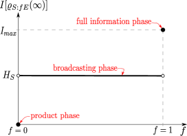
Figure 3: (Color online) Information-theoretical phases of the sphere model (cf. sfera_zurek ). Schematic phase diagram, showing three different phases of the illuminated sphere model, appearing in the thermodynamic and the deep decoherence $t\gg\tau_{D}$ limits. The horizontal axis is the observed fraction $f$ of the total photon number, understood modulo a microfraction. The vertical axis is the asymptotic mutual information between the sphere $S$ and the fraction $fE$, $I[\varrho_{S:fE}(\infty)]$. This is the limiting diagram for those from sfera_zurek obtained for finite $t$. There are two phase transitions: At $f=0$ from the singular product phase (represented by the black point at zero) to the broadcasting phase (the black line at $H_{S}$); and at $f=1$ from the broadcasting phase to the singular full information phase (black dot at $I_{max}$).

Conversely, if we have access to the full environment, ignoring perhaps only a microscopic fraction $\mu$, the arguments leading to Eqs. (44,48) do not work anymore, since from Eq. (52):

$$\left|{\rm Tr}{\bf S}_{1}\varrho^{ph}_{0}{\bf S}_{2}^{\dagger}\right|^{\mu}\xrightarrow{\text{therm.}}1,$$ (55)

and thus there is no decoherence nor orthogonalization. The post-scattering state contains then the full quantum information about the system due to the unsuppressed system-environment entanglement produced by the controlled-unitary interaction (26). As a result, the mutual information attains in the thermodynamical limit its maximum value $I_{max}=2H_{S}$ (for a pure $\varrho_{0}^{S}$, since the interaction is of a controlled unitary form (26)) and this defines the full information phase. We note that the rise of $I_{S:fE}$ above $H_{S}$ certifies the presence of entanglement entropic . The intermediate phase described by Eq. (49) is the broadcasting phase (see Fig. 3).

The quantity experiencing discontinuous jumps is the mutual information between the system $S$ and the observed environment $fE$, and the parameter which drives the phase transitions is the fraction size $f$. As discussed above, each value of $f$ has to be understood modulo a micro-fraction. The appearance of the phase diagram is a reflection of both the thermodynamic and the deep decoherence limits and its form is in agreement with the previously obtained results (see e.g. Refs. sfera_zurek ; RiedelZurek ).

A.4 Derivation of the entropic objectivity condition in the illuminated sphere model

Here we present an independent derivation of the entropic objectivity condition

$$I[\varrho_{S:fE}(t)]\approx H_{S},$$ (56)

for the illuminated sphere model. Although illustrated on a concrete model, our derivation is indeed more general—instead of a direct, asymptotic calculation of the mutual information $I[\varrho_{S:fE}(t)]$ in the model (cf. Refs. ZwolakZurek ; sfera_zurek ; RiedelZurek ), we will show that Eq. (56) follows from the mechanisms of: i) decoherence, Eq. (34), and ii) distinguishability, Eq. (36), once they are proven. In light of our findings, this puts a clear physical meaning to Eq. (56)—it is a consequence of the state information broadcasting. Most of the proof is for general, mixed states.

Let the post-interaction $S:fE$ state for a fixed, finite box $L$ and time $t$ be $\varrho_{S:fE}(L,t)$. It is given by Eqs. (32,33) and now we explicitly indicate the dependence on $L$ in the notation. Then:

$$\left|H_{S}-I\left[\varrho_{S:fE}(L,t)\right]\right|\leq$$

$$\left|I\left[\varrho_{S:fE}(L,t)\right]-I\left[\varrho^{i=j}_{S:fE}(L,t)\right]\right|$$ (57)

$$+\left|H_{S}-I\left[\varrho^{i=j}_{S:fE}(L,t)\right]\right|,$$ (58)

where $\varrho^{i=j}_{S:fE}(L,t)$ is the decohered part of $\varrho_{S:fE}(L,t)$, given by Eq. (32). We first bound the difference (57), decomposing the mutual information using conditional information $S_{\text{vN}}(\varrho_{S:fE}|\varrho_{fE})\equiv S_{\text{vN}}(\varrho_{S:fE})-S_{\text{vN}}(\varrho_{fE})$:

$$I(\varrho_{S:fE})=S_{\text{vN}}\left(\varrho_{S}\right)-S_{\text{vN}}\left(\varrho_{S:fE}|\varrho_{fE}\right),$$ (59)

so that:

$$\left|I\left[\varrho_{S:fE}(L,t)\right]-I\left[\varrho^{i=j}_{S:fE}(L,t)\right]\right|\leq$$

$$\left|S_{\text{vN}}\left[\varrho_{S}(L,t)\right]-S_{\text{vN}}\left[\varrho^{i=j}_{S}(L,t)\right]\right|+$$ (60)

$$\Big{|}S_{\text{vN}}\left[\varrho_{S:fE}(L,t)\big{|}\varrho_{fE}(L,t)\right]$$

$$\quad\quad\quad\quad\quad-S_{\text{vN}}\left[\varrho_{S:fE}^{i=j}(L,t)\Big{|}\varrho_{fE}^{i=j}(L,t)\right]\Big{|}.$$ (61)

>From Eq. (23), the total $S:fE$ Hilbert space is finite-dimensional for a finite $L,t$: there are $fN_{t}=$$fL^{2}(N/V)ct$ photons (cf. Eq. (25)) and the number of modes of each photon is approximately $(4\pi/3)(L/2\pi\Delta x)^{3}$. Hence, the total dimension is $2\times L^{2}f(N/V)ct\times(1/6\pi^{2})(L/\Delta x)^{3}<\infty$ and we can use the Fannes-Audenaert FAd and the Alicki-Fannes FannesAlicki inequalities to bound (60) and (61) respectively (cf. Ref. ZwolakZurek ). For (60) we obtain:

$$\left|S_{\text{vN}}\left[\varrho_{S}(L,t)\right]-S_{\text{vN}}\left[\varrho^{i=j}_{S}(L,t)\right]\right|$$

$$\leq\frac{1}{2}\epsilon_{E}(L,t)\log(d_{S}-1)+h\left[\frac{\epsilon_{E}(L,t)}{2}\right],$$ (62)

where $h(\epsilon)\equiv-\epsilon\log\epsilon-(1-\epsilon)\log(1-\epsilon)$ is the binary Shannon entropy and:

$$\epsilon_{E}(L,t)\equiv||\varrho_{S}(L,t)-\varrho^{i=j}_{S}(L,t)||_{tr}$$ (63)

$$=||\varrho^{i\neq j}_{S}(L,t)||_{tr}\cong 2|c_{12}|\left[1-\frac{1}{c\tau_{D}L^{2}}\left(\frac{N}{V}\right)^{-1}\right]^{L^{2}\frac{N}{V}ct}$$ (64)

with $c_{12}\equiv\langle\vec{x}_{1}|\varrho^{S}_{0}\,\vec{x}_{2}\rangle$, where we have used the reasoning (39-44), but with $f=0$. For (61) the same reasoning and the Alicki-Fannes inequality give:

$$\left|S_{\text{vN}}\left[\varrho_{S:fE}(L,t)\big{|}\varrho_{fE}(L,t)\right]-S_{\text{vN}}\left[\varrho_{S:fE}^{i=j}(L,t)\big{|}\varrho_{fE}^{i=j}(L,t)\right]\right|$$

$$\leq 4\epsilon_{fE}(L,t)\log d_{S}+2h\left[\epsilon_{fE}(L,t)\right],$$ (65)

with:

$$\epsilon_{fE}(L,t) \equiv ||\varrho_{S:fE}(L,t)-\varrho^{i=j}_{S:fE}(L,t)||_{tr}$$ (66)

$$= ||\varrho^{i\neq j}_{S:fE}(L,t)||_{tr}$$ (67)

$$\cong 2|c_{12}|\left[1-\frac{1}{c\tau_{D}L^{2}}\left(\frac{N}{V}\right)^{-1}\right]^{L^{2}(1-f)\frac{N}{V}ct}.$$ (68)

Above $L,t$ are big enough so that $\epsilon_{E}(L,t),\epsilon_{fE}(L,t)<1$. Eqs. (60-68) give an upper bound on the difference (57) in terms of the decoherence speed (34).

To bound the "orthogonalization" part (58) (see Ref. ZwolakZurek for a related analysis), we note that since $\varrho^{i=j}_{S:fE}(L,t)$ is a CQ-state (cf. Eq. (32)), its mutual information is given by the Holevo quantity Holevo :

$$I\left[\varrho^{i=j}_{S:fE}(L,t)\right]=\chi\left\{p_{i},\varrho_{i}^{mac}(t)^{\otimes fM}\right\},$$ (69)

where $p_{i}$ is given by Eq. (37). >From the Holevo Theorem it is bounded by Holevo :

$$I_{max}(t)\leq\chi\left\{p_{i},\varrho_{i}^{mac}(t)^{\otimes fM}\right\}\leq H\left(\{p_{i}\}\right)\equiv H_{S},$$ (70)

where $I_{max}(t)\equiv\max_{\mathcal{E}}I[p_{i}\pi^{\mathcal{E}}_{j|i}(t)]$ is the fixed time maximal mutual information, extractable through generalized measurements $\{\mathcal{E}_{j}\}$ on the ensemble $\{p_{i},\varrho_{i}^{mac}(t)^{\otimes fM}\}$, and the conditional probabilities read:

$$\pi^{\mathcal{E}}_{j|i}(t)\equiv{\rm Tr}[\mathcal{E}_{j}\varrho_{i}^{mac}(t)^{\otimes fM}]$$ (71)

(here and below $i$ labels the states, while $j$ the measurement outcomes). We now relate $I_{max}(t)$ to the generalized overlap $B\left[\varrho_{1}^{mac}(t)^{\otimes fM},\varrho_{2}^{mac}(t)^{\otimes fM}\right]$ (cf. Eq. (36)), which we have calculated for pure states in Eq. (47,48). Using the method of Ref. Fuchs , slightly modified to unequal a priori probabilities $p_{i}$, we obtain for an arbitrary measurement $\mathcal{E}$:

$$I\left(\pi^{\mathcal{E}}_{j|i}p_{i}\right)=I\left(\pi^{\mathcal{E}}_{i|j}\pi^{\mathcal{E}}_{j}\right)=H\left(\{p_{i}\}\right)-\sum_{j=1,2}\pi^{\mathcal{E}}_{j}h\left(\pi^{\mathcal{E}}_{1|j}\right)$$

(72)

$$\geq H\left(\{p_{i}\}\right)-2\sum_{j=1,2}\pi^{\mathcal{E}}_{j}\sqrt{\pi^{\mathcal{E}}_{1|j}\left(1-\pi^{\mathcal{E}}_{1|j}\right)}$$ (73)

$$=H\left(\{p_{i}\}\right)-2\sqrt{p_{1}p_{2}}\sum_{j=1,2}\sqrt{\pi^{\mathcal{E}}_{j|1}\pi^{\mathcal{E}}_{j|2}},$$ (74)

where we have first used Bayes Theorem $\pi^{\mathcal{E}}_{i|j}=(p_{i}/\pi^{\mathcal{E}}_{j})\pi^{\mathcal{E}}_{j|i}$, $\pi^{\mathcal{E}}_{j}\equiv\sum_{i}\pi^{\mathcal{E}}_{j|i}p_{i}={\rm Tr}(\mathcal{E}_{j}\sum_{i}\varrho_{i})$, then the fact that we have only two states: $\pi^{\mathcal{E}}_{2|j}=1-\pi^{\mathcal{E}}_{1|j}$, so that $H(\pi^{\mathcal{E}}_{\cdot|j})=h(\pi^{\mathcal{E}}_{1|j})$, and finally $h(p)\leq 2\sqrt{p(1-p)}$. On the other hand, $B(\varrho_{1},\varrho_{2})=\min_{\mathcal{E}}\sum_{j}\sqrt{\pi^{\mathcal{E}}_{j|1}\pi^{\mathcal{E}}_{j|2}}$ Fuchs . Denoting the optimal measurement by $\mathcal{E}_{*}^{B}(t)$ and recognizing that $H(\{p_{i}\})=H_{S}$, we obtain:

$$I_{max}(t)\geq I\left[p_{i}\pi^{\mathcal{E}_{*}^{B}(t)}_{j|i}(t)\right]\geq H_{S}-$$ (75)

$$-2\sqrt{p_{1}p_{2}}\,B\left[\varrho_{1}^{mac}(t)^{\otimes fM},\varrho_{2}^{mac}(t)^{\otimes fM}\right]$$ (76)

$$=H_{S}-2\sqrt{p_{1}p_{2}}\,B\left[\varrho^{mac}_{1}(t),\varrho^{mac}_{2}(t)\right]^{fM}$$ (77)

Inserting the above into the bounds (70) gives the desired upper bound on the difference (58):

$$\left|H_{S}-I\left[\varrho^{i=j}_{S:fE}(L,t)\right]\right|\leq 2\sqrt{p_{1}p_{2}}\,B\left[\varrho^{mac}_{1}(t),\varrho^{mac}_{2}(t)\right]^{fM}$$

where the generalized overlap is given by Eqs. (47,48):

$$B\left[\varrho^{mac}_{1}(t),\varrho^{mac}_{2}(t)\right]=\left|\langle\Psi_{2}^{mac}(t)|\Psi_{1}^{mac}(t)\rangle\right|\cong$$

$$\quad\quad\quad\left[1-\frac{1}{c\tau_{D}L^{2}}\left(\frac{N}{V}\right)^{-1}\right]^{L^{2}m\frac{N}{V}ct}.$$ (79)

Gathering all the above facts together finally leads to a bound on $\left|H_{S}-I\left[\varrho_{S:fE}(L,t)\right]\right|$ in terms of the speed of i) decoherence (34) and ii) distinguishability (36):

$$\left|H_{S}-I\left[\varrho_{S:fE}(L,t)\right]\right|\leq h\left[\frac{\epsilon_{E}(L,t)}{2}\right]+2h\left[\epsilon_{fE}(L,t)\right]+$$

(80)

$$4\epsilon_{fE}(L,t)\log 2+2\sqrt{p_{1}p_{2}}\,B\left[\varrho^{mac}_{1}(t),\varrho^{mac}_{2}(t)\right]^{fM},$$ (81)

where $\epsilon_{E}(L,t)$, $\epsilon_{fE}(L,t)$, $B\left[\varrho^{mac}_{1}(t),\varrho^{mac}_{2}(t)\right]$ are given by Eqs. (64), (68), and (79) respectively. Choosing $L,t$ big enough so that $\epsilon_{E}(L,t),\epsilon_{fE}(L,t)\leq 1/2$ (when the binary entropy $h(\cdot)$ is monotonically increasing), we remove the unphysical box and obtain an estimate on the speed of convergence of $I\left[\varrho_{S:fE}(L,t)\right]$ to $H_{S}$:

$$\lim_{L\to\infty}\left|H_{S}-I\left[\varrho_{S:fE}(L,t)\right]\right|\leq h\left(|c_{12}|\text{e}^{-\frac{t}{\tau_{D}}}\right)$$ (82)

$$+2h\left(2|c_{12}|\text{e}^{-\frac{(1-f)}{\tau_{D}}t}\right)+8|c_{12}|\text{e}^{-\frac{(1-f)}{\tau_{D}}t}\log 2$$ (83)

$$+2\sqrt{p_{1}p_{2}}\text{e}^{-\frac{f}{\tau_{D}}t}.$$ (84)

This finishes the derivation of the condition (56).

We note that the result (80,81) is in fact a general statement, valid in any model where: i) the system $S$ is effectively a qubit; ii) the system-environment interaction is of a environment-symmetric controlled-unitary type:

Lemma 2

Let a two-dimensional quantum system $S$ interact with $N$ identical environments, each described by a $d$-dimensional Hilbert space, through a controlled-unitary interaction:

$$U(t)\equiv\sum_{i=1,2}|i\rangle\langle i|\otimes U_{i}(t)^{\otimes N}.$$ (85)

Let the initial state be $\varrho_{S:E}(0)=\varrho_{0}^{S}\otimes(\varrho_{0}^{E})^{\otimes N}$ and $\varrho_{S:E}(t)\equiv U(t)\varrho_{S:E}(0)U(t)^{\dagger}$. Then for any $0<f<1$ and $t$ big enough:

$$\left|H(\{p_{i}\})-I\left[\varrho_{S:fE}(t)\right]\right|\leq h\left[\frac{\epsilon_{E}(t)}{2}\right]+2h\left[\epsilon_{fE}(t)\right]+$$

(86)

$$4\epsilon_{fE}(t)\log 2+2\sqrt{p_{1}p_{2}}\,B\left[\varrho_{1}(t),\varrho_{2}(t)\right]^{fN},$$ (87)

where:

$$p_{i}\equiv\langle i|\varrho_{0}^{S}|i\rangle,\,\varrho_{i}(t)\equiv U_{i}(t)\varrho_{0}^{E}U_{i}(t)^{\dagger},$$ (88)

$$\epsilon_{E}(t)\equiv||\varrho_{S}(t)-\varrho^{i=j}_{S}||_{tr},$$ (89)

$$\epsilon_{fE}(t)\equiv||\varrho_{S:fE}(t)-\varrho^{i=j}_{S:fE}(t)||_{tr}.$$ (90)

References

- (1) N. Bohr, ”Discussions with Einstein on Epistemological Problems in Atomic Physics” in P. A. Schilpp (Ed.), Albert Einstein: Philosopher-Scientist, Library of Living Philosophers, Evanston, Illinois (1949).
- (2) W. Heisenberg, Philosophic Problems in Nuclear Science (F. C. Hayes Transl.), (Faber and Faber, London, 1952).
- (3) Joos E, et al., Decoherence and the Appearancs of a Classical World in Quantum Theory (Springer, Berlin, 2003).
- (4) H. D. Zeh in Quantum Decoherence, Eds. Duplantier B, Raimond J-M, Rivasseau V, (Birkhäuser, Basel, 2006).
- (5) M. Schlosshauer, Decoherence and the Quantum-to-Classical Transition (Springer, Berlin, 2007).
- (6) W. H. Zurek, Phys. Rev. D 24, 1516 (1981).
- (7) W. H. Zurek, Nature Phys. 5, 181 (2009).
- (8) W. Wootters, W. H. Zurek, Nature 299, 802 (1982).
- (9) M. Zwolak, W. H. Zurek, Sci. Rep. 3, 1729 (2013).
- (10) M. Zwolak, H. T. Quan, and W. H. Zurek, Phys. Rev. A 81, 062110 (2010).
- (11) C. J. Riedel, W. H. Zurek, Phys. Rev. Lett. 105, 020404 (2010).
- (12) F. G. S. L. Brandao, M. Piani, and P. Horodecki, arXiv:1310.8640 (2013).
- (13) T. Y. Cao, Conceptual Developments of 20th Century Field Theories, Cambridge University Press, Cambridge (1997).
- (14) N. Bohr, Phys. Rev. 48, 696 (1935).
- (15) H. M. Wiseman, Ann. Phys. 338, 361 (2013).
- (16) A. Einstein, B. Podolsky, and N. Rosen, Phys. Rev. 47, 777 (1935).
- (17) E. Joos, H. D. Zeh, Z. Phys. B 59, 223 (1985).
- (18) J. K. Korbicz, P. Horodecki, and R. Horodecki, Phys. Rev. Lett. 112, 120402 (2014).
- (19) R. Blume-Kohout, W. H. Zurek, Phys. Rev. A 73, 062310 (2006).
- (20) H. Ollivier, D. Poulin, and W. H. Zurek, Phys. Rev. Lett. 93, 220401 (2004).
- (21) J. Oppenheim, M. Horodecki, P. Horodecki, and R. Horodecki, Phys. Rev. Lett. 89, 180402 (2002).
- (22) M. Piani, P. Horodecki, and R. Horodecki, Phys. Rev. Lett. 100, 090502 (2008).
- (23) J. K. Korbicz, P. Horodecki, R. Horodecki, Phys. Rev. A 86, 042319 (2012).
- (24) W. H. Zurek, Phys. Rev. A 87, 052111 (2013).
- (25) K. Modi, A. Brodutch, H. Cable, T. Paterek, and V. Vedral, Rev. Mod. Phys. 84, 1655 (2012).
- (26) P. Horodecki, R. Horodecki, Quant. Inf. Comp. 1, 45 (2001).
- (27) H. Barnum, C. M. Caves, C. A. Fuchs, R. Jozsa, and B. Schumacher, Phys. Rev. Lett. 76, 2818 (1996).
- (28) T. M. Cover, J. A. Thomas, Elements of Information Theory (John Wiley and Sons, New York, 1991).
- (29) M. Horodecki, J. Oppenheim, A. Winter, Nature 436, 673 (2005).
- (30) A. Peres, Phys. Rev. Lett. 77, 1413 (1996); M. Horodecki, P. Horodecki, R. Horodecki, Phys. Lett. A 223, 1 (1996).
- (31) K. M. R. Audenaert, J. Phys. A: Math. Theor. 40, 8127 (2007).
- (32) R. Alicki, M. Fannes, J. Phys. A: Math. Gen. 37, L55, (2004).
- (33) Paris M, Řeháček J Eds. , Quantum State Estimation, Lect. Notes Phys. 649 (Springer, Berlin, 2004).
- (34) M. F. Pusey, J. Barrett, T. Rudolph, Nature Phys. 8, 476 (2012).
- (35) J. Bell, Physics 1, 195 (1964).
- (36) E. P. Wigner, in The Logic of Personal Knowledge: Essays Presented to Michael Polany on his Seventieth Birthday (Routledge & Kegan Paul, London, 1961).
- (37) M. R. Gallis, and G. N. Fleming, Phys. Rev. A 42, 38 (1990).
- (38) C. J. Riedel, and W. H. Zurek, New J. Phys. 13, 073038 (2011).
- (39) K. Hornberger, and J. E. Sipe Phys. Rev. A 68, 012105 (2003).
- (40) S. L. Adler, J. Phys. A 39, 14067 (2006).
- (41) G. Sewell, Rep. Math. Phys. 56, 271 (2005).
- (42) C. A. Fuchs, and J. van de Graaf IEEE Trans. on Inf. Theor. 45, 1216 (1999).
- (43) R. Horodecki, and P. Horodecki, Phys. Lett. A 194, 147 (1994).
- (44) A. S. Holevo, Problm. Inform. Transm. 9, 177 (1973).