The Connectivity of Boolean Satisfiability: Dichotomies for Formulas and Circuits

Abstract

For Boolean satisfiability problems, the structure of the solution space is characterized by the solution graph, where the vertices are the solutions, and two solutions are connected iff they differ in exactly one variable. In 2006, Gopalan et al. studied connectivity properties of the solution graph and related complexity issues for CSPs [11], motivated mainly by research on satisfiability algorithms and the satisfiability threshold. They proved dichotomies for the diameter of connected components and for the complexity of the $st$-connectivity question, and conjectured a trichotomy for the connectivity question. Recently, we were able to establish the trichotomy [23].

Here, we consider connectivity issues of satisfiability problems defined by Boolean circuits and propositional formulas that use gates, resp. connectives, from a fixed set of Boolean functions. We obtain dichotomies for the diameter and the two connectivity problems: On one side, the diameter is linear in the number of variables, and both problems are in P, while on the other side, the diameter can be exponential, and the problems are PSPACE-complete. For partially quantified formulas, we show an analogous dichotomy.

Keywords   Computational Complexity $\cdot$ Boolean Satisfiability$\cdot$ Boolean Circuits $\cdot$ Post’s Lattice $\cdot$ PSPACE-Completeness $\cdot$ Dichotomy Theorems $\cdot$ Graph Connectivity

Institut für Theoretische Informatik, Leibniz Universität Hannover,
Appelstr. 4, 30167 Hannover, Germany
k.w.s@gmx.net

1   Introduction

The Boolean satisfiability problem (SAT), as well as many related questions like equivalence, counting, enumeration, and numerous versions of optimization, are of great importance in both theory and applications of computer science. In this article, we focus on the solution-space structure: We consider the solution graph, where the vertices are the solutions, and two solutions are connected iff they differ in exactly one variable. For this implicitly defined graph, we then study the connectivity and $st$-connectivity problems, and the diameter of connected components. The figures below give an impression of how solution graphs may look like.

            

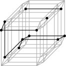
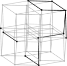
Figure 1: Depictions of the subgraph of the 5-dimensional hypercube graph induced by a typical random Boolean relation with 12 elements. Left: highlighted on a orthographic hypercube projection. Center: highlighted on a “Spectral Embedding” of the hypercube graph by Mathematica. Right: the sole subgraph, arranged by Mathematica

            

Figure 2: Subgraphs of the 8-dimensional hypercube graph induced by typical random relations with 40, 60 and 80 elements, arranged by Mathematica.

While the standard satisfiability problem is defined for propositional formulas, which can be seen as one special form of descriptions for Boolean relations, satisfiability and related problems have also been considered for many alternative descriptions, e.g. Boolean constraint satisfactions problems (CSPs), Boolean circuits, binary decision diagrams, and Boolean neural networks. For the usual formulas with the connectives $\wedge$, $\vee$ and $\neg$, there are several common variants. A special form are formulas in conjunctive normal form (CNF-formulas). A generalization of CNF-formulas are CNF($\mathcal{S}$)-formulas, which are conjunctions of constraints on the variables taken from a finite template set $\mathcal{S}$.

Here we consider another type of generalization: Arbitrarily nested formulas built with connectives from some finite set of Boolean functions $B$ (where the arity may be greater than two), known as $B$-formulas. Also we study $B$-circuits, where analogously the allowed gates implement the functions from $B$. As a further extension we consider partially quantified $B$-formulas.

A direct application of $st$-connectivity in solution graphs are reconfiguration problems, that arise when we wish to find a step-by-step transformation between two feasible solutions of a problem, such that all intermediate results are also feasible. Recently, the reconfiguration versions of many problems such as Independent-Set, Vertex-Cover, Set-Cover Graph-$k$-Coloring, Shortest-Path have been studied, and complexity results obtained (see e.g. [12, 13]). Also of relevance are the connectivity properties to the problem of structure identification, where one is given a relation explicitly and seeks a short representation of some kind (see e.g. [5]); this problem is important especially for learning in artificial intelligence.

A better understanding of the solution space structure also promises advancement of SAT algorithms: It has been discovered that the solution space connectivity is strongly correlated to the performance of standard satisfiability algorithms like WalkSAT and DPLL on random instances: As one approaches the satisfiability threshold (the ratio of constraints to variables at which random $k$-CNF-formulas become unsatisfiable for $k\geq 3$) from below, the solution space (with the connectivity defined as above) fractures, and the performance of the algorithms deteriorates [16, 15]. These insights mainly came from statistical physics, and lead to the development of the survey propagation algorithm, which has much better performance on random instances [15].

While current SAT solvers normally accept only CNF-formulas as input, one of the most important applications of satisfiability testing is verification and optimization in Electronic Design Automation (EDA), where the instances derive mostly from digital circuit descriptions [27]. Though many such instances can easily be encoded in CNF, the original structural information, such as signal ordering, gate orientation and logic paths, is lost, or at least obscured. Since exactly this information can be very helpful for solving these instances, considerable effort has been made recently to develop satisfiability solvers that work with the circuit description directly [27], which have far superior performance in EDA applications, or to restore the circuit structure from CNF [8]. This is a major motivation for our study.

Our perspective is mainly from complexity theory: We classify $B$-formulas and $B$-circuits by the worst-case complexity of the connectivity problems, analogously to Schaefer’s dichotomy theorem for satisfiability of CSPs from 1978 [21], Lewis’ dichotomy for satisfiability of $B$-formulas from 1979 [14], and Gopalan et al.’s classification for the connectivity problems of CSPs from 2006 [11]. Along the way, we will examine structural properties of the solution graph like its maximal diameter, and devise efficient algorithms for solving the connectivity problems.

We begin with a formal definition of some central concepts.

Definition 1.

An $n$-ary Boolean relation is a subset of $\{0,1\}^{n}$ ($n\geq 1$). If $\phi$ is some description of an $n$-ary Boolean relation $R$, e.g. a propositional formula (where the variables are taken in lexicographic order), the solution graph $G(\phi)$ of $\phi$ is the subgraph of the $n$-dimensional hypercube graph induced by the vectors in $R$, i.e., the vertices of $G(\phi$) are the vectors in $R$, and there is an edge between two vectors precisely if they differ in exactly one position.

We use $\boldsymbol{a},\boldsymbol{b},\ldots$ to denote vectors of Boolean values and $\boldsymbol{x},\boldsymbol{y},\ldots$ to denote vectors of variables, $\boldsymbol{a}=(a_{1},a_{2},\ldots)$ and $\boldsymbol{x}=(x_{1},x_{2},\ldots)$.

The Hamming weight $|\boldsymbol{a}|$ of a Boolean vector $\boldsymbol{a}$ is the number of 1’s in $\boldsymbol{a}$. For two vectors $\boldsymbol{a}$ and $\boldsymbol{b}$, the Hamming distance $|\boldsymbol{a}-\boldsymbol{b}|$ is is the number of positions in which they differ.

If $\boldsymbol{a}$ and $\boldsymbol{b}$ are solutions of $\phi$ and lie in the same connected component of $G(\phi)$, we write $d_{\phi}(\boldsymbol{a},\boldsymbol{b})$ to denote the shortest-path distance between $\boldsymbol{a}$ and $\boldsymbol{b}$.

The diameter of a connected component is the maximal shortest-path distance between any two vectors in that component. The diameter of $G(\phi)$ is the maximal diameter of any of its connected components.

2   Connectivity of CNF-Formulas

Research has focused on the structure of the solution space only quite recently: One of the earliest studies on solution-space connectivity was done for CNF($\mathcal{S}$)-formulas with constants (see the definition below), begun in 2006 by Gopalan et al. ([10], [18], [11], [23]).

In our proofs for $B$-formulas and $B$-circuits, we will use Gopalan et al.’s results for 3-CNF-formulas, so we have to introduce some related terminology.

Definition 2.

A CNF-formula is a Boolean formula of the form $C_{1}\wedge\cdots\wedge C_{m}$ ($1\leq m<\infty$), where each $C_{i}$ is a clause, that is, a finite disjunction of literals (variables or negated variables). A $k$-CNF-formula ($k\geq 1$) is a CNF-formula where each $C_{i}$ has at most $k$ literals.

For a finite set of Boolean relations $\mathcal{S}$, a CNF($\mathcal{S}$)-formula (with constants) over a set of variables $V$ is a finite conjunction $C_{1}\wedge\cdots\wedge C_{m}$, where each $C_{i}$ is a constraint application (constraint for short), i.e., an expression of the form $R(\xi_{1},\ldots,\xi_{k})$, with a $k$-ary relation $R\in\mathcal{S}$, and each $\xi_{j}$ is a variable in $V$ or one of the constants 0, 1.

A $k$-clause is a disjunction of $k$ variables or negated variables. For $0\leq i\leq k$, let $D_{i}$ be the set of all satisfying truth assignments of the $k$-clause whose first $i$ literals are negated, and let $S_{k}=\{D_{0},\ldots,D_{k}\}$. Thus, CNF($S_{k}$) is the collection of $k$-CNF-formulas.

Gopalan et al. studied the following two decision problems for CNF($\mathcal{S}$)-formulas:

• the connectivity problem Conn($\mathcal{S}$): given a CNF($\mathcal{S}$)-formula $\phi$, is $G(\phi)$ connected? (if $\phi$ is unsatisfiable, then $G(\phi)$ is considered connected)

• the $st$-connectivity problem st-Conn($\mathcal{S}$): given a CNF($\mathcal{S}$)-formula $\phi$ and two solutions $\boldsymbol{s}$ and $\boldsymbol{t}$, is there a path from $\boldsymbol{s}$ to $\boldsymbol{t}$ in $G(\phi)$?

Lemma 3.

[11, Lemm 3.6] st-Conn($S_{3}$) and Conn($S_{3}$) are $\mathrm{PSPACE}$-complete.

Showing that the problems are in PSPACE is straightforward: Given a CNF($S_{3}$)-formula $\phi$ and two solutions $\boldsymbol{s}$ and $\boldsymbol{t}$, we can guess a path of length at most $2^{n}$ between them and verify that each vertex along the path is indeed a solution. Hence st-Conn($S_{3}$) is in $\mathrm{NPSPACE}$, which equals PSPACE by Savitch’s theorem. For Conn($S_{3}$), by reusing space we can check for all pairs of vectors whether they are satisfying, and, if they both are, whether they are connected in $G(\phi)$.

The hardness-proof is quite intricate: it consists of a direct reduction from the computation of a space-bounded Turing machine $M$. The input-string $w$ of $M$ is mapped to a CNF($S_{3}$)-formula $\phi$ and two satisfying assignments $\boldsymbol{s}$ and $\boldsymbol{t}$, corresponding to the initial and accepting configuration of a Turing machine $M^{\prime}$ constructed from $M$ and $w$, s.t. $\boldsymbol{s}$ and $\boldsymbol{t}$ are connected in $G(\phi)$ iff $M$ accepts $w$. Further, all satisfying assignments of $\phi$ are connected to either $\boldsymbol{s}$ or $\boldsymbol{t}$, so that $G(\phi)$ is connected iff $M$ accepts $w$.

Lemma 4.

[11, Lemm 3.7] For $n\geq 2$ , there is an $n$-ary Boolean function $f$ with $f(1,\ldots,1)=1$ and a diameter of at least $2^{\left\lfloor\frac{n}{2}\right\rfloor}$.

The proof of this lemma is by direct construction of such a formula.

3   Circuits, Formulas, and Post’s Lattice

An $n$-ary Boolean function is a function $f:\{0,1\}^{n}\rightarrow\{0,1\}$. Let $B$ be a finite set of Boolean functions.

A $B$-circuit $\mathcal{C}$ with input variables $x_{1},\ldots,x_{n}$ is a directed acyclic graph, augmented as follows: Each node (here also called gate) with indegree 0 is labeled with an $x_{i}$ or a 0-ary function from $B$, each node with indegree $k>0$ is labeled with a $k$-ary function from $B$. The edges (here also called wires) pointing into a gate are ordered. One node is designated the output gate. Given values $a_{1},\ldots,a_{n}\in\{0,1\}$ to $x_{1},\ldots,x_{n}$, $\mathcal{C}$ computes an $n$-ary function $f_{\mathcal{C}}$ as follows: A gate $v$ labeled with a variable $x_{i}$ returns $a_{i}$, a gate $v$ labeled with a function $f$ computes the value $f(b_{1},\ldots,b_{k})$, where $b_{1},\ldots,b_{k}$ are the values computed by the predecessor gates of $v$, ordered according to the order of the wires. For a more formal definition see [26].

A $B$-formula is defined inductively: A variable $x$ is a $B$-formula. If $\phi_{1},\ldots,\phi_{m}$ are $B$-formulas, and $f$ is an $n$-ary function from $B$, then $f(\phi_{1},\ldots,\phi_{n})$ is a $B$-formula. In turn, any $B$-formula defines a Boolean function in the obvious way, and we will identify $B$-formulas and the function they define.

It is easy to see that the functions computable by a $B$-circuit, as well as the functions definable by a $B$-formula, are exactly those that can be obtained from $B$ by superposition, together with all projections [3]. By superposition, we mean substitution (that is, composition of functions), permutation and identification of variables, and introduction of fictive variables (variables on which the value of the function does not depend). This class of functions is denoted by $[B]$. $B$ is closed (or said to be a clone) if $[B]=B$. A base of a clone $F$ is any set $B$ with $[B]=F$.

Already in the early 1920s, Emil Post extensively studied Boolean functions [19]. He identified all clones, found a finite base for each of them, and detected their inclusion structure: The clones form a lattice, called Post’s lattice, depicted in Figure 3.

The following clones are defined by properties of the functions they contain, all other ones are intersections of these. Let $f$ be an $n$-ary Boolean function.

• $\mathsf{BF}$ is the class of all Boolean functions.

• $\mathsf{R}_{0}$ ($\mathsf{R}_{1}$) is the class of all 0-reproducing (1-reproducing) functions,
  $f$ is $c$-reproducing, if $f(c,\ldots,c)=c$, where $c\in\{0,1\}$.

• $\mathsf{M}$ is is the class of all monotone functions,
  $f$ is monotone, if $a_{1}\leq b_{1},\ldots,a_{n}\leq b_{n}$ implies $f(a_{1},\ldots,a_{n})\leq f(b_{1},\ldots,b_{n})$.

• $\mathsf{D}$ is the class of all self-dual functions,
  $f$ is self-dual, if $f(x_{1},\ldots,x_{n})=\overline{f(\overline{x_{1}},\ldots,\overline{x_{n}})}$.

• $\mathsf{L}$ is the class of all affine (on linear) functions,
  $f$ is affine, if $f(x_{1},\ldots,x_{n})=x_{i_{1}}\oplus\cdots\oplus x_{i_{m}}\oplus c$ with $i_{1},\ldots,i_{m}\in\{1,\ldots,n\}$ and $c\in\{0,1\}$.

• $\mathsf{S}_{0}$ ($\mathsf{S}_{1}$) is the class of all 0-separating (1-separating) functions,
  $f$ is $c$-separating, if there exists an $i\in\{1,\ldots,n\}$ s.t. $a_{i}=c$ for all $\boldsymbol{a}\in f^{-1}(c)$, where $c\in\{0,1\}$.

• $\mathsf{S}_{0}^{m}$ ($\mathsf{S}_{1}^{m}$) is the class of all functions that are 0-separating (1-separating) of degree $m$,
  $f$ is $c$-separating of degree $m$, if for all $U\subseteq f^{-1}(c)$ of size $|U|=m$ there exists an $i\in\{1,\ldots,n\}$ s.t. $a_{i}=c$ for all $\boldsymbol{a}\in U$ ($c\in\{0,1\}$, $m\geq 2$).

The definitions and bases of all classes are given in Table 1. For an introduction to Post’s lattice and further references see e.g. [3].

Figure 3: Graphical representation of Post’s lattice.
The classes on the hard side of the dichotomy for the connectivity problems and the diameter are shaded gray; the light gray shaded ones are only on the hard side for formulas with quantifiers.
For comparison, the classes for which SAT (without quantifiers) is NP-complete are circled bold.

Class	Definition	Base
$\mathsf{BF}$	All Boolean functions	$\{x\land y,\neg x\}$
$\mathsf{R}_{0}$	$\{f\in\mathsf{BF}\mid f\mbox{ is 0-reproducing}\}$	$\{x\land y,x\oplus y\}$
$\mathsf{R}_{1}$	$\{f\in\mathsf{BF}\mid f\mbox{ is 1-reproducing}\}$	$\{x\lor y,x\leftrightarrow y\}$
$\mathsf{R}_{2}$	$\mathsf{R}_{0}\cap\mathsf{R}_{1}$	$\{x\lor y,x\land(y\leftrightarrow z)\}$
$\mathsf{M}$	$\{f\in\mathsf{BF}\mid f\mbox{ is monotone}\}$	$\{x\land y,x\lor y,0,1\}$
$\mathsf{M}_{0}$	$\mathsf{M}\cap\mathsf{R}_{0}$	$\{x\land y,x\lor y,0\}$
$\mathsf{M}_{1}$	$\mathsf{M}\cap\mathsf{R}_{1}$	$\{x\land y,x\lor y,1\}$
$\mathsf{M}_{2}$	$\mathsf{M}\cap\mathsf{R}_{2}$	$\{x\land y,x\lor y\}$
$\mathsf{S}_{0}$	$\{f\in\mathsf{BF}\mid f\mbox{ is 0-separating}\}$	$\{x\rightarrow y\}$
$\mathsf{S}_{0}^{n}$	$\{f\in\mathsf{BF}\mid f\mbox{ is 0-separating of degree $n$}\}$	$\{x\rightarrow y,\mbox{dual}({\mathrm{T}^{n+1}_{n}})\}$
$\mathsf{S}_{1}$	$\{f\in\mathsf{BF}\mid f\mbox{ is 1-separating}\}$	$\{x\nrightarrow y\}$
$\mathsf{S}_{1}^{n}$	$\{f\in\mathsf{BF}\mid f\mbox{ is 1-separating of degree $n$}\}$	$\{x\nrightarrow y,\mathrm{T}^{n+1}_{n}\}$
$\mathsf{S}_{02}^{n}$	$\mathsf{S}_{0}^{n}\cap\mathsf{R}_{2}$	$\{x\lor(y\land\neg z),\mbox{dual}({\mathrm{T}^{n+1}_{n}})\}$
$\mathsf{S}_{02}$	$\mathsf{S}_{0}\cap\mathsf{R}_{2}$	$\{x\lor(y\land\neg z)\}$
$\mathsf{S}_{01}^{n}$	$\mathsf{S}_{0}^{n}\cap\mathsf{M}$	$\{\mbox{dual}({\mathrm{T}^{n+1}_{n}}),1\}$
$\mathsf{S}_{01}$	$\mathsf{S}_{0}\cap\mathsf{M}$	$\{x\lor(y\land z),1\}$
$\mathsf{S}_{00}^{n}$	$\mathsf{S}_{0}^{n}\cap\mathsf{R}_{2}\cap\mathsf{M}$	$\{x\lor(y\land z),\mbox{dual}({\mathrm{T}^{n+1}_{n}})\}$
$\mathsf{S}_{00}$	$\mathsf{S}_{0}\cap\mathsf{R}_{2}\cap\mathsf{M}$	$\{x\lor(y\land z)\}$
$\mathsf{S}_{12}^{n}$	$\mathsf{S}_{1}^{n}\cap\mathsf{R}_{2}$	$\{x\land(y\lor\neg z),\mathrm{T}^{n+1}_{n}\}$
$\mathsf{S}_{12}$	$\mathsf{S}_{1}\cap\mathsf{R}_{2}$	$\{x\land(y\lor\neg z)\}$
$\mathsf{S}_{11}^{n}$	$\mathsf{S}_{1}^{n}\cap\mathsf{M}$	$\{\mathrm{T}^{n+1}_{n},0\}$
$\mathsf{S}_{11}$	$\mathsf{S}_{1}\cap\mathsf{M}$	$\{x\land(y\lor z),0\}$
$\mathsf{S}_{10}^{n}$	$\mathsf{S}_{1}^{n}\cap\mathsf{R}_{2}\cap\mathsf{M}$	$\{x\land(y\lor z),{\mathrm{T}^{n+1}_{n}}\}$
$\mathsf{S}_{10}$	$\mathsf{S}_{1}\cap\mathsf{R}_{2}\cap\mathsf{M}$	$\{x\land(y\lor z)\}$
$\mathsf{D}$	$\{f\in\mathsf{BF}\mid f\mbox{ is self-dual}\}$	$\{\mbox{maj}(x,\neg y,\neg z)\}$
$\mathsf{D}_{1}$	$\mathsf{D}\cap\mathsf{R}_{2}$	$\{\mbox{maj}(x,y,\neg z)\}$
$\mathsf{D}_{2}$	$\mathsf{D}\cap\mathsf{M}$	$\{\mbox{maj}(x,y,z)\}$
$\mathsf{L}$	$\{f\in\mathsf{BF}\mid f\mbox{ is linear}\}$	$\{x\oplus y,1\}$
$\mathsf{L}_{0}$	$\mathsf{L}\cap\mathsf{R}_{0}$	$\{x\oplus y\}$
$\mathsf{L}_{1}$	$\mathsf{L}\cap\mathsf{R}_{1}$	$\{x\leftrightarrow y\}$
$\mathsf{L}_{2}$	$\mathsf{L}\cap\mathsf{R}_{2}$	$\{x\oplus y\oplus z\}$
$\mathsf{L}_{3}$	$\mathsf{L}\cap\mathsf{D}$	$\{x\oplus y\oplus z\oplus 1\}$
$\mathsf{E}$	$\{f\in\mathsf{BF}\mid f\mbox{ is constant or a conjunction}\}$	$\{x\land y,0,1\}$
$\mathsf{E}_{0}$	$\mathsf{E}\cap\mathsf{R}_{0}$	$\{x\land y,0\}$
$\mathsf{E}_{1}$	$\mathsf{E}\cap\mathsf{R}_{1}$	$\{x\land y,1\}$
$\mathsf{E}_{2}$	$\mathsf{E}\cap\mathsf{R}_{2}$	$\{x\land y\}$
$\mathsf{V}$	$\{f\in\mathsf{BF}\mid f\mbox{ is constant or a disjunction}\}$	$\{x\lor y,0,1\}$
$\mathsf{V}_{0}$	$\mathsf{V}\cap\mathsf{R}_{0}$	$\{x\lor y,0\}$
$\mathsf{V}_{1}$	$\mathsf{V}\cap\mathsf{R}_{1}$	$\{x\lor y,1\}$
$\mathsf{V}_{2}$	$\mathsf{V}\cap\mathsf{R}_{2}$	$\{x\lor y\}$
$\mathsf{N}$	$\{f\in\mathsf{BF}\mid f\mbox{ is essentially unary}\}$	$\{\neg x,0,1\}$
$\mathsf{N}_{2}$	$\mathsf{N}\cap\mathsf{D}$	$\{\neg x\}$
$\mathsf{I}$	$\{f\in\mathsf{BF}\mid f\mbox{ is constant or a projection}\}$	$\{x,0,1\}$
$\mathsf{I}_{0}$	$\mathsf{I}\cap\mathsf{R}_{0}$	$\{x,0\}$
$\mathsf{I}_{1}$	$\mathsf{I}\cap\mathsf{R}_{1}$	$\{x,1\}$
$\mathsf{I}_{2}$	$\mathsf{I}\cap\mathsf{R}_{2}$	$\{x\}$

Table 1: List of all closed classes of Boolean functions with definitions and bases.
($T_{k}^{n}$ denotes the threshold function, $T_{k}^{n}(x_{1},\ldots,x_{n})=1\Longleftrightarrow\sum_{i=1}^{n}x_{i}\geq k$, and dual($f$)$(x_{1},\ldots,x_{n})=\overline{f(\overline{x_{1}},\ldots,\overline{x_{n}})}$)

The complexity of numerous problems for $B$-circuits and $B$-formulas has been classified by the types of functions allowed in $B$ with help of Post’s lattice (see e.g. [20, 22]), starting with satisfiability: Analogously to Schaefer’s dichotomy for CNF($\mathcal{S}$)-formulas from 1978, Harry R. Lewis shortly thereafter found a dichotomy for $B$-formulas [14]: If $[B]$ contains the function $x\wedge\overline{y}$, Sat is NP-complete, else it is in P.

While for $B$-circuits the complexity of every decision problem solely depends on $[B]$ (up to AC⁰ isomorphisms), for $B$-formulas this need not be the case (though it usually is, as for satisfiability and our connectivity problems, as we will see): The transformation of a $B$-formula into a $B^{\prime}$-formula might require an exponential increase in the formula size even if $[B]=[B^{\prime}]$, as the $B^{\prime}$-representation of some function from $B$ may need to use some input variable more than once [25]. For example, let $h(x,y)=x\wedge\overline{y}$; then $(\text{x$\wedge$y)}\in[\{h\}]$ since $x\wedge y=h(x,h(x,y))$, but it is easy to see that there is no shorter $\{h\}$-representation of $x\wedge y$.

4   Computational and Structural Dichotomies for Connectivity

Now we consider the connectivity problems for $B$-formulas and $B$-circuits:

• BF-Conn($B$): Given a $B$-formula $\phi$, is $G(\phi)$ connected?

• st-BF-Conn($B$): Given a $B$-formula $\phi$ and two solutions $\boldsymbol{s}$ and $\boldsymbol{t}$, is there a path from $\boldsymbol{s}$ to $\boldsymbol{t}$ in $G(\phi)$?

The corresponding problems for circuits are denoted Circ-Conn($B$) resp. st-Circ-Conn($B$).

Theorem 5.

Let $B$ be a finite set of Boolean functions.

1. If $B\subseteq\mathsf{M}$, $B\subseteq\mathsf{L}$, or $B\subseteq\mathsf{\mathsf{S}_{0}}$, then

   1. st-Circ-Conn($B$) and Circ-Conn($B$) are in P,

      1. st-BF-Conn($B$) and BF-Conn($B$) are in P,

      2. the diameter of every function $f\in[B]$ is linear in the number of variables of $f$.

   2. Otherwise,

      1. st-Circ-Conn($B$) and Circ-Conn($B$) are $\mathrm{PSPACE}$-complete,

      2. st-BF-Conn($B$) and BF-Conn($B$) are $\mathrm{PSPACE}$-complete,

      3. there are functions $f\in[B]$ such that their diameter is exponential in the number of variables of $f$.

The proof follows from the Lemmas in the next subsections. By the following proposition, we can relate the complexity of $B$-formulas and $B$-circuits.

Proposition 6.

Every $B$-formula $\phi$ can be transformed into an equivalent $B$-circuit $\mathcal{C}$ in polynomial time.

Proof.

Any $B$-formula is equivalent to a special $B$-circuit where all function-gates have outdegree at most one: For every variable $x$ of $\phi$ and for every occurrence of a function $f$ in $\phi$ there is a gate in $\mathcal{C}$, labeled with $x$ resp. $f$. It is clear how to connect the gates. ∎

4.1   The Easy Side of the Dichotomy

Lemma 7.

If $B\subseteq\mathsf{M}$, the solution graph of any $n$-ary function $f\in[B]$ is connected, and $d_{f}(\boldsymbol{a},\boldsymbol{b})=|\boldsymbol{a}-\boldsymbol{b}|\leq n$ for any two solutions $\boldsymbol{a}$ and $\boldsymbol{b}$.

Proof.

Table 1 shows that $f$ is monotone in this case. Thus, either $f=0$, or $(1,\ldots,1)$ must be a solution, and every other solution $\boldsymbol{a}$ is connected to $(1,\ldots,1)$ in $G(\phi)$ since $(1,\ldots,1)$ can be reached by flipping the variables assigned 0 in $\boldsymbol{a}$ one at a time to 1. Further, if $\boldsymbol{a}$ and $\boldsymbol{b}$ are solutions, $\boldsymbol{b}$ can be reached from $\boldsymbol{a}$ in $|\boldsymbol{a}-\boldsymbol{b}|$ steps by first flipping all variables that are assigned 0 in $\boldsymbol{a}$ and 1 in $\boldsymbol{b}$, and then flipping all variables that are assigned 1 in $\boldsymbol{a}$ and 0 in $\boldsymbol{b}$.∎

Lemma 8.

If $B\subseteq\mathsf{S}_{0}$, the solution graph of any function $f\in[B]$ is connected, and $d_{f}(\boldsymbol{a},\boldsymbol{b})\leq|\boldsymbol{a}-\boldsymbol{b}|+2$ for any two solutions $\boldsymbol{a}$ and $\boldsymbol{b}$.

Proof.

Since $f$ is 0-separating, there is an $i$ such that $a_{i}=0$ for every vector $\boldsymbol{a}$ with $f(\boldsymbol{a})=0$, thus every $\boldsymbol{b}$ with $b_{i}=1$ is a solution. It follows that every solution $\boldsymbol{t}$ can be reached from any solution $\boldsymbol{s}$ in at most $|\boldsymbol{s}-\boldsymbol{t}|+2$ steps by first flipping the $i$-th variable from 0 to 1 if necessary, then flipping all other variables in which $\boldsymbol{s}$ and $\boldsymbol{t}$ differ, and finally flipping back the $i$-th variable if necessary.∎

Lemma 9.

If $B\subseteq\mathsf{L}$,

1. st-Circ-Conn($B$) and Circ-Conn($B$) are in P,

   1. st-BF-Conn($B$) and BF-Conn($B$) are in P,

   2. for any function $f\in[B]$, $d_{f}(\boldsymbol{a},\boldsymbol{b})=|\boldsymbol{a}-\boldsymbol{b}|$ for any two solutions $\boldsymbol{a}$ and $\boldsymbol{b}$ that lie in the same connected component of $G(\phi)$.

Proof.

Since every function $f\in\mathsf{L}$ is linear, $f(x_{1},\ldots,x_{n})=x_{i_{1}}\oplus\ldots\oplus x_{i_{m}}\oplus c$, and any two solutions $\boldsymbol{s}$ and $\boldsymbol{t}$ are connected iff they differ only in fictive variables: If $\boldsymbol{s}$ and $\boldsymbol{t}$ differ in at least one non-fictive variable (i.e., an $x_{i}\in\{x_{i_{1}},\ldots,x_{i_{m}}\}$), to reach $\mathbf{t}$ from $\mathbf{s}$, $x_{i}$ must be flipped eventually, but for every solution $\boldsymbol{a}$, any vector $\boldsymbol{b}$ that differs from $\boldsymbol{a}$ in exactly one non-fictive variable is no solution. If $\boldsymbol{s}$ and $\boldsymbol{t}$ differ only in fictive variables, $\boldsymbol{t}$ can be reached from $\boldsymbol{s}$ in $|\boldsymbol{s}-\boldsymbol{t}|$ steps by flipping one by one the variables in which they differ.

Since $\{x\oplus y,1\}$ is a base of $\mathsf{L}$, every $B$-circuit $\mathcal{C}$ can be transformed in polynomial time into an equivalent $\{x\oplus y,1\}$-circuit $\mathcal{C}^{\prime}$ by replacing each gate of $\mathcal{C}$ with an equivalent $\{x\oplus y,1\}$-circuit. Now one can decide in polynomial time whether a variable $x_{i}$ is fictive by checking for $\mathcal{C}^{\prime}$ whether the number of “backward paths” from the output gate to gates labeled with $x_{i}$ is odd, so st-Circ-Conn($B$) is in P.

$G(\mathcal{C})$ is connected iff at most one variable is non-fictive, thus Circ-Conn($B$) is in P.

By Proposition 6, st-BF-Conn($B$) and BF-Conn($B$) are in P also. ∎

This completes the proof of the easy side of the dichotomy.

4.2   The Hard Side of the Dichotomy

Proposition 10.

st-Circ-Conn($B$) and Circ-Conn($B$), as well as st-BF-Conn($B$) and BF-Conn($B$), are in $\mathrm{PSPACE}$ for any finite set $B$ of Boolean functions.

Proof.

This follows as in Lemma 3.6 of [11] (see Lemma 3). ∎

An inspection of Post’s lattice shows that if $B\nsubseteq\mathsf{M}$, $B\nsubseteq\mathsf{L}$, and $B\nsubseteq\mathsf{S}_{0}$, then $[B]\supseteq\mathsf{S}_{12}$, $[B]\supseteq\mathsf{D}_{1}$, or $[B]\supseteq\mathsf{S}_{02}^{k}\,\forall k\geq 2$, so we have to prove $\mathrm{PSPACE}$-completeness and show the existence of $B$-formulas with an exponential diameter in these cases.

In the proofs, we will use the following notation: We write $\boldsymbol{x}=\boldsymbol{c}$ or $\boldsymbol{x}=c_{1}\cdots c_{n}$ for $(x_{1}=c_{1})\wedge\cdots\wedge(x_{n}=c_{n})$, where $\boldsymbol{c}=(c_{1},\ldots,c_{n})$ is a vector of constants; e.g., $\boldsymbol{x}=\boldsymbol{0}$ means $\overline{x}_{1}\wedge\cdots\wedge\overline{x}_{n}$, and $\boldsymbol{x}=101$ means $x_{1}\wedge\overline{x}_{2}\wedge x_{3}$. Further, we use $\boldsymbol{x}\in\left\{\boldsymbol{a},\boldsymbol{b},\ldots\right\}$ for $(\boldsymbol{x}=\boldsymbol{a})\vee(\boldsymbol{x}=\boldsymbol{b})\vee\ldots$. Also, we write $\psi(\boldsymbol{\overline{x}})$ for $\psi(\overline{x}_{1},\ldots,\overline{x}_{n})$. If we have two vectors of Boolean values $\boldsymbol{a}$ and $\boldsymbol{b}$ of length $n$ and $m$ resp., we write $\boldsymbol{a}\cdot\boldsymbol{b}$ for their concatenation $(a_{1},\ldots,a_{n},b_{1},\ldots b_{m})$.

All hardness proofs are by reductions from the problems for 1-reproducing 3-CNF-formulas, which are $\mathrm{PSPACE}$-complete by the following proposition.

Proposition 11.

For 1-reproducing 3-CNF-formulas, the problems st-Conn and Conn are $\mathrm{PSPACE}$-complete.

Proof.

In the $\mathrm{PSPACE}$-hardness proof for CNF($S_{3}$)-formulas (Lemma 3.6 of [11], see Lemma 3), two satisfying assignments $\boldsymbol{s}$ and $\boldsymbol{t}$ to the constructed formula $\phi$ are known, so we can construct a connectivity-equivalent 1-reproducing 3-CNF-formula $\psi$, e.g. as $\psi(\boldsymbol{x})=\phi(x_{1}\oplus s_{1}\oplus 1,\ldots,x_{n}\oplus s_{n}\oplus 1)$, and then check connectivity for $\psi$ instead of $\phi$.∎∎

Lemma 12.

If $[B]\supseteq\mathsf{S}_{12}$,

1. st-BF-Conn($B$) and BF-Conn($B$) are $\mathrm{PSPACE}$-complete,

   1. st-Circ-Conn($B$) and Circ-Conn($B$) are $\mathrm{PSPACE}$-complete,

   2. for $n\geq 3$, there is an $n$-ary function $f\in[B]$ with diameter of at least $2^{\left\lfloor\frac{n-1}{2}\right\rfloor}$.

Proof.

1. We reduce the problems for 1-reproducing 3-CNF-formulas to the ones for $B$-formulas: We map a 1-reproducing 3-CNF-formula $\phi$ and two solutions $\boldsymbol{s}$ and $\boldsymbol{t}$ of $\phi$ to a $B$-formula $\phi^{\prime}$ and two solutions $\boldsymbol{s^{\prime}}$ and $\boldsymbol{t^{\prime}}$ of $\phi^{\prime}$ such that $\boldsymbol{s^{\prime}}$ and $\boldsymbol{t^{\prime}}$ are connected in $G(\phi^{\prime})$ iff $\boldsymbol{s}$ and $\boldsymbol{t}$ are connected in $G(\phi)$, and such that $G(\phi^{\prime})$ is connected iff $G(\phi)$ is connected.

While the construction of $\phi^{\prime}$ is quite easy for this lemma, the construction for the next two lemmas is analogous but more intricate, so we proceed carefully in two steps, which we will adapt in the next two proofs: In the first step, we give a transformation $T$ that transforms any 1-reproducing formula $\psi$ into a connectivity-equivalent formula $T_{\psi}\in\mathsf{S}_{12}$ built from the standard connectives. Since $\mathsf{S}_{12}\subseteq[B]$, we can express $T_{\psi}$ as a $B$-formula $T_{\psi}^{*}$. Now if we would apply $T$ to $\phi$ directly, we would know that $T_{\phi}$ can be expressed as a $B$-formula. However, this could lead to an exponential increase in the formula size (see Section 3), so we have to show how to construct the $B$-formula in polynomial time. For this, in the second step, we construct a $B$-formula $\phi^{\prime}$ directly from $\phi$ (by applying $T$ to the clauses and the $\wedge$’s individually), and then show that $\phi^{\prime}$ is equivalent to $T_{\phi}$; thus we know that $\phi^{\prime}$ is connectivity-equivalent to $\phi$.

Step 1. From Table 1, we find that $\mathsf{S}_{12}=\mathsf{S}_{1}\cap\mathsf{R}_{2}=\mathsf{S}_{1}\cap\mathsf{R}_{0}\cap\mathsf{R}_{1}$, so we have to make sure that $T_{\psi}$ is 1-seperating, 0-reproducing, and 1-reproducing. Let

$$T_{\psi}=\psi\wedge y,$$

where $y$ is a new variable.

All solutions $\boldsymbol{a}$ of $T_{\psi}(\boldsymbol{x},y)$ have $a_{n+1}=1$, so $T_{\psi}$ is 1-seperating and 0-reproducing; also, $T_{\psi}$ is still 1-reproducing. Further, for any two solutions $\boldsymbol{s}$ and $\boldsymbol{t}$ of $\psi(\boldsymbol{x})$, $\boldsymbol{s}^{\prime}=\boldsymbol{s}\cdot 1$ and $\boldsymbol{t}^{\prime}=\boldsymbol{t}\cdot 1$ are solutions of $T_{\psi}(\boldsymbol{x},y)$, and it is easy to see that they are connected in $G(T_{\psi})$ iff $\boldsymbol{s}$ and $\boldsymbol{t}$ are connected in $G(\psi)$, and that $G(T_{\psi})$ is connected iff $G(\psi)$ is connected.

Step 2. The idea is to parenthesize the conjunctions of $\phi$ such that we get a tree of $\wedge$’s of depth logarithmic in the size of $\phi$, and then to replace each clause and each $\wedge$ with an equivalent $B$-formula. This can increase the formula size by only a polynomial in the original size even if the $B$-formula equivalent to $\wedge$ uses some input variable more than once.

Let $\phi=C_{1}\wedge\cdots\wedge C_{n}$ be a 1-reproducing 3-CNF-formula. Since $\phi$ is 1-reproducing, every clause $C_{i}$ of $\phi$ is itself 1-reproducing, and we can express $T_{C_{i}}$ through a $B$-formula $T_{C_{i}}^{*}$. Also, we can express $T_{u\wedge v}$ through a $B$-formula $T_{u\wedge v}^{*}$ since $\wedge$ is 1-reproducing; we write $T_{\wedge}(\psi_{1},\psi_{2})$ for the formula obtained from $T_{u\wedge v}$ by substituting the formula $\psi_{1}$ for $u$ and $\psi_{2}$ for $v$, and similarly write $T_{\wedge}^{*}(\psi_{1},\psi_{2})$ for the formula obtained from $T_{u\wedge v}^{*}$ in this way. We let $\phi^{\prime}=$Tr$(\phi)$, where Tr is the following recursive algorithm that takes a CNF-formula as input:

Algorithm Tr$\left(\psi_{1}\wedge\cdots\wedge\psi_{m}\right)$∎

• If $m=1$, return $T_{\psi_{1}}^{*}$.

• Else return $T_{\wedge}^{*}\left(\textsc{Tr}(\psi_{1}\wedge\cdots\wedge\psi_{\left\lfloor m/2\right\rfloor}),\textsc{Tr}(\psi_{\left\lfloor m/2\right\rfloor+1}\wedge\cdots\wedge\psi_{m})\right)$.

Proof.

Since the recursion terminates after a number of steps logarithmic in the number of clauses of $\phi$, and every step increases the total formula size by only a constant factor, the algorithm runs in polynomial time. We show $\phi^{\prime}\equiv T_{\phi}$ by induction on $m$. For $m=1$ this is clear. For the induction step, we have to show $T_{\wedge}^{*}(T_{\psi_{1}},T_{\psi_{2}})\equiv T_{\psi_{1}\wedge\psi_{2}}$, but since $T_{\wedge}(\psi_{1},\psi_{2})\equiv T_{\wedge}^{*}(\psi_{1},\psi_{2})$, it suffices to show that $T_{\wedge}(T_{\psi_{1}},T_{\psi_{2}})\equiv T_{\psi_{1}\wedge\psi_{2}}$:

$$T_{\wedge}(T_{\psi_{1}},T_{\psi_{2}})=(\psi_{1}\wedge y)\wedge(\psi_{2}\wedge y)\wedge y\equiv\psi_{1}\wedge\psi_{2}\wedge y=T_{\psi_{1}\wedge\psi_{2}}.$$

2. This follows from 1. by Proposition 6.

3. By Lemma 4, there is an 1-reproducing $(n-1)$-ary function $f$ with diameter of at least $2^{\left\lfloor\frac{n-1}{2}\right\rfloor}$. Let $f$ be represented by a formula $\phi$; then, $T_{\phi}$ represents an $n$-ary function of the same diameter in $\mathsf{S}_{12}$.∎

Lemma 13.

If $[B]\supseteq\mathsf{D}_{1}$,

1. st-BF-Conn($B$) and BF-Conn($B$) are $\mathrm{PSPACE}$-complete,

   1. st-Circ-Conn($B$) and Circ-Conn($B$) are $\mathrm{PSPACE}$-complete,

   2. for $n\geq 5$, there is an $n$-ary function $f\in[B]$ with diameter of at least $2^{\left\lfloor\frac{n-3}{2}\right\rfloor}$.

Proof.

1. As noted, we adapt the two steps from the previous proof.

Step 1. Since $\mathsf{D}_{1}=\mathsf{D}\cap\mathsf{R}_{0}\cap\mathsf{R}_{1}$, $T_{\psi}$ must be self-dual, 0-reproducing, and 1-reproducing. For clarity, we first construct an intermediate formula $T_{\psi}^{\sim}\in\mathsf{D}_{1}$ whose solution graph has an additional component, then we eliminate that component.

For $\psi(\boldsymbol{x})$, let

$$T_{\psi}^{\sim}=\left(\psi(\boldsymbol{x})\wedge(\boldsymbol{y}=\boldsymbol{1})\right)\vee\left(\overline{\psi(\boldsymbol{\overline{x}})}\wedge(\boldsymbol{y}=\boldsymbol{0})\right)\vee\left(\boldsymbol{y}\in\left\{100,010,001\right\}\right),$$

where $\boldsymbol{y}=(y_{1},y_{2},y_{3})$ are three new variables.

$T_{\psi}^{\sim}$ is self-dual: for any solution ending with 111 (satisfying the first disjunct), the inverse vector is no solution; similarly, for any solution ending with 000 (satisfying the second disjunct), the inverse vector is no solution; finally, all vectors ending with 100, 010, or 001 are solutions and their inverses are no solutions. Also, $T_{\psi}^{\sim}$ is still 1-reproducing, and it is 0-reproducing (for the second disjunct note that $\overline{\psi(\overline{0\cdots 0})}\equiv\overline{\psi(1\cdots 1)}\equiv 0$).

Further, every solution $\boldsymbol{a}$ of $\psi$ corresponds to a solution $\boldsymbol{a}\cdot 111$ of $T_{\psi}^{\sim}$, and for any two solutions $\boldsymbol{s}$ and $\boldsymbol{t}$ of $\psi$, $\boldsymbol{s}^{\prime}=\boldsymbol{s}\cdot 111$ and $\boldsymbol{t}^{\prime}=\boldsymbol{t}\cdot 111$ are connected in $G(T_{\psi}^{\sim})$ iff $\boldsymbol{s}$ and $\boldsymbol{t}$ are connected in $G(\psi)$: The “if” is clear, for the “only if” note that since there are no solutions of $T_{\psi}^{\sim}$ ending with 110, 101, or 011, every solution of $T_{\psi}^{\sim}$ not ending with 111 differs in at least two variables from the solutions that do.

Observe that exactly one connected component is added in $G(T_{\psi}^{\sim})$ to the components corresponding to those of $G(\psi)$: It consists of all solutions ending with 000, 100, 010, or 001 (any two vectors ending with 000 are connected e.g. via those ending with 100). It follows that $G(T_{\psi}^{\sim})$ is always unconnected. To fix this, we modify $T_{\psi}^{\sim}$ to $T_{\psi}$ by adding $1\cdots 1\cdot 110$ as a solution, thereby connecting $1\cdots 1\cdot 111$ (which is always a solution since $T_{\psi}^{\sim}$ is 1-reproducing) with $1\cdots 1\cdot 100$, and thereby with the additional component of $T_{\psi}$. To keep the function self-dual, we must in turn remove $0\cdots 0\cdot 001$, which does not alter the connectivity. Formally,

$$T_{\psi} = \left(T_{\psi}^{\sim}\vee\left((\boldsymbol{x}=\boldsymbol{1})\wedge(\boldsymbol{y}=110)\right)\right)\wedge\neg\left((\boldsymbol{x}=\boldsymbol{0})\wedge(\boldsymbol{y}=001)\right)$$

$$= \left(\psi(\boldsymbol{x})\wedge(\boldsymbol{y}=\boldsymbol{1})\right)\vee\left(\overline{\psi(\boldsymbol{\overline{x}})}\wedge(\boldsymbol{y}=\boldsymbol{0})\right)$$

$$\vee\left(\boldsymbol{y}\in\left\{100,010,001\right\}\wedge\neg((\boldsymbol{x}=\boldsymbol{0})\wedge(\boldsymbol{y}=001))\right)$$

$$\vee((\boldsymbol{x}=\boldsymbol{1})\wedge(\boldsymbol{y}=110)).$$

            

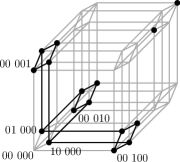
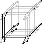
Figure 4: An example for the transformation. Left: $\psi=\left(x_{1}\vee\overline{x_{2}}\right)\wedge\left(\overline{x_{1}}\vee x_{2}\right)$, center: $T_{\psi}^{\sim}$, right: $T_{\psi}$. The “axis vertices” are labeled in the first two graphs.

Now $G(T_{\psi})$ is connected iff $G(\psi)$ is connected.

Step 2. Again, we use the algorithm Tr from the previous proof to transform any 1-reproducing 3-CNF-formula $\phi$ into a $B$-formula $\phi^{\prime}$ equivalent to $T_{\phi}$, but with the definition (4.2) of $T$. Again, we have to show $T_{\wedge}(T_{\psi_{1}},T_{\psi_{2}})\equiv T_{\psi_{1}\wedge\psi_{2}}$. Here,

$$T_{\wedge}(T_{\psi_{1}},T_{\psi_{2}}) = \left(T_{\psi_{1}}\wedge T_{\psi_{2}}\wedge(\boldsymbol{y}=\boldsymbol{1})\right)\vee\left(\overline{\overline{T_{\psi_{1}}}\wedge\overline{T_{\psi_{2}}}}\wedge(\boldsymbol{y}=\boldsymbol{0})\right)$$

$$\vee\left(\boldsymbol{y}\in\left\{100,010,001\right\}\wedge\neg\left(\overline{T_{\psi_{1}}}\wedge\overline{T_{\psi_{2}}}\wedge(\boldsymbol{y}=001)\right)\right)$$

$$\vee\left(T_{\psi_{1}}\wedge T_{\psi_{2}}\wedge(\boldsymbol{y}=110)\right).$$

We consider the parts of the formula in turn: For any formula $\xi$ we have $T_{\xi}(\boldsymbol{x}_{\xi})\wedge(\boldsymbol{y}=\boldsymbol{1})\equiv\xi(\boldsymbol{x}_{\xi})\wedge(\boldsymbol{y}=\boldsymbol{1})$ and $T_{\xi}(\boldsymbol{x}_{\xi})\wedge(\boldsymbol{y}=\boldsymbol{0})\equiv\overline{\psi(\overline{\boldsymbol{x}_{\xi}})}\wedge(\boldsymbol{y}=\boldsymbol{0})$, where $\boldsymbol{x}_{\xi}$ denotes the variables of $\xi$. Using $\overline{\overline{T_{\psi_{1}}(\boldsymbol{x}_{\psi_{1}})}\wedge\overline{T_{\psi_{2}}(\boldsymbol{x}_{\psi_{2}})}}\wedge(\boldsymbol{y}=\boldsymbol{0})=\left(T_{\psi_{1}}(\boldsymbol{x}_{\psi_{1}})\vee T_{\psi_{2}}(\boldsymbol{x}_{\psi_{2}})\right)\wedge(\boldsymbol{y}=\boldsymbol{0})$, the first line becomes

$$\left(\psi_{1}(\boldsymbol{x}_{\psi_{1}})\wedge\psi_{2}(\boldsymbol{x}_{\psi_{2}})\wedge(\boldsymbol{y}=\boldsymbol{1})\right)\vee\left(\left(\overline{\psi_{1}(\overline{\boldsymbol{x}_{\psi_{1}}})\wedge\psi_{2}(\overline{\boldsymbol{x}_{\psi_{2}}})}\right)\wedge(\boldsymbol{y}=\boldsymbol{0})\right).$$

For the second line, we observe

$$\overline{T_{\psi}(\boldsymbol{x}_{\psi})} \equiv \left(\overline{\psi(\boldsymbol{x}_{\psi})}\vee\neg(\boldsymbol{y}=\boldsymbol{1})\right)\wedge\left(\psi(\boldsymbol{\overline{x}_{\psi}})\vee\neg(\boldsymbol{y}=\boldsymbol{0})\right)$$

$$\wedge\left(\boldsymbol{y}\notin\left\{100,010,001\right\}\vee\left((\boldsymbol{x}_{\psi}=\boldsymbol{0})\wedge(\boldsymbol{y}=001)\right)\right)$$

$$\wedge(\neg(\boldsymbol{x}_{\psi}=\boldsymbol{1})\vee\overline{(\boldsymbol{y}=110)}),$$

thus $\overline{T_{\psi}(\boldsymbol{x}_{\psi})}\wedge(\boldsymbol{y}=001)\equiv(\boldsymbol{x}_{\psi}=\boldsymbol{0})\wedge(\boldsymbol{y}=001)$, and the second line becomes

$$\vee\left(\boldsymbol{y}\in\left\{100,010,001\right\}\wedge\neg\left((\boldsymbol{x}_{\psi_{1}}=\boldsymbol{0})\wedge(\boldsymbol{x}_{\psi_{2}}=\boldsymbol{0})\wedge(\boldsymbol{y}=001)\right)\right).$$

Since $T_{\psi}(\boldsymbol{x}_{\psi})\wedge(\boldsymbol{y}=110)\equiv(\boldsymbol{x}_{\psi}=\boldsymbol{1})\wedge(\boldsymbol{y}=110)$ for any $\psi$, the third line becomes

$$\vee\left((\boldsymbol{x}_{\psi_{1}}=\boldsymbol{1})\wedge(\boldsymbol{x}_{\psi_{2}}=\boldsymbol{1})\wedge(\boldsymbol{y}=110)\right).$$

Now $T_{\wedge}(T_{\psi_{1}},T_{\psi_{2}})$ equals

$$T_{\psi_{1}\wedge\psi_{2}} = \left(\psi_{1}(\boldsymbol{x}_{\psi_{1}})\wedge\psi_{2}(\boldsymbol{x}_{\psi_{2}})\wedge(\boldsymbol{y}=\boldsymbol{1})\right)\vee\left(\overline{\psi_{1}(\overline{\boldsymbol{x}_{\psi_{1}}})\wedge\psi_{2}(\overline{\boldsymbol{x}_{\psi_{2}}})}\wedge(\boldsymbol{y}=\boldsymbol{0})\right)$$

$$\vee\left(\boldsymbol{y}\in\left\{100,010,001\right\}\wedge\neg\left((\boldsymbol{x}_{\psi_{1}}=\boldsymbol{0})\wedge(\boldsymbol{x}_{\psi_{2}}=\boldsymbol{0})\wedge(\boldsymbol{y}=001)\right)\right)$$

$$\vee\left((\boldsymbol{x}_{\psi_{1}}=\boldsymbol{1})\wedge(\boldsymbol{x}_{\psi_{2}}=\boldsymbol{1})\wedge(\boldsymbol{y}=110)\right).$$

2. This follows from 1. by Proposition 6.

3. By Lemma 4 there is an 1-reproducing $(n-3)$-ary function $f$ with diameter of at least $2^{\left\lfloor\frac{n-3}{2}\right\rfloor}$. Let $f$ be represented by a formula $\phi$; then, $T_{\phi}$ represents an $n$-ary function of the same diameter in $\mathsf{D}_{1}$.∎

Lemma 14.

If $[B]\supseteq\mathsf{S}_{02}^{k}$ for any $k\geq 2$,

1. st-BF-Conn($B$) and BF-Conn($B$) are $\mathrm{PSPACE}$-complete,

   1. st-Circ-Conn($B$) and Circ-Conn($B$) are $\mathrm{PSPACE}$-complete,

   2. for $n\geq k+4$, there is an $n$-ary function $f\in[B]$ with diameter of at least $2^{\left\lfloor\frac{n-k-2}{2}\right\rfloor}$.

Proof.

1. Step 1. Since $\mathsf{S}_{02}^{k}=\mathsf{S}_{0}^{k}\cap\mathsf{R}_{0}\cap\mathsf{R}_{1}$, $T_{\psi}$ must be 0-separating of degree $k$, 0-reproducing, and 1-reproducing. As in the previous proof, we construct an intermediate formula $T_{\psi}^{\sim}$. For $\psi(\boldsymbol{x})$, let

$$T_{\psi}^{\sim}=\left(\psi\wedge y\wedge(\boldsymbol{z}=\boldsymbol{0})\right)\vee(|\boldsymbol{z}|>1),$$

where $y$ and $\boldsymbol{z}=(z_{1},\ldots,z_{k+1})$ are new variables.

$T_{\psi}^{\sim}(\boldsymbol{x},y,\boldsymbol{z})$ is 0-separating of degree $k$, since all vectors that are no solutions of $T_{\psi}^{\sim}$ have $|\boldsymbol{z}|\leq 1$, i.e. $\boldsymbol{z}\in\left\{0\cdots 0,10\cdots 0,010\cdots 0,\ldots,0\cdots 01\right\}\subset\{0,1\}^{k+1}$, and thus any $k$ of them have at least one common variable assigned 0. Also, $T_{\psi}^{\sim}$ is 0-reproducing and still 1-reproducing.

Further, for any two solutions $\boldsymbol{s}$ and $\boldsymbol{t}$ of $\psi(\boldsymbol{x})$, $\boldsymbol{s}^{\prime}=\boldsymbol{s}\cdot 1\cdot 0\cdots 0$ and $\boldsymbol{t}^{\prime}=\boldsymbol{t}\cdot 1\cdot 0\cdots 0$ are solutions of $T_{\psi}^{\sim}(\boldsymbol{x},y,\boldsymbol{z})$ and are connected in $G(T_{\psi}^{\sim})$ iff $\boldsymbol{s}$ and $\boldsymbol{t}$ are connected in $G(\psi)$.

But again, we have produced an additional connected component (consisting of all solutions with $|\boldsymbol{z}|>1$). To connect it to a component corresponding to one of $\psi$, we add $1\cdots 1\cdot 1\cdot 10\cdots 0$ as a solution,

$$T_{\psi} = \left(\psi\wedge y\wedge(\boldsymbol{z}=\boldsymbol{0})\right)\vee(|\boldsymbol{z}|>1)\vee\left((\boldsymbol{x}=\boldsymbol{1})\wedge y\wedge(\boldsymbol{z}=10\cdots 0)\right).$$

Now $G(T_{\psi})$ is connected iff $G(\psi)$ is connected.

Step 2. Again we show that the algorithm Tr works in this case. Here,

$$T_{\wedge}(T_{\psi_{1}},T_{\psi_{2}}) = \left(T_{\psi_{1}}(\boldsymbol{x}_{\psi_{1}})\wedge T_{\psi_{2}}(\boldsymbol{x}_{\psi_{2}})\wedge y\wedge(\boldsymbol{z}=\boldsymbol{0})\right)\vee(|\boldsymbol{z}|>1)$$

$$\vee\left(T_{\psi_{1}}(\boldsymbol{x}_{\psi_{1}})\wedge T_{\psi_{2}}(\boldsymbol{x}_{\psi_{2}})\wedge y\wedge(\boldsymbol{z}=10\cdots 0)\right).$$

Since $T_{\psi}(\boldsymbol{x}_{\psi})\wedge y\wedge(\boldsymbol{z}=\boldsymbol{0})\equiv\psi(\boldsymbol{x}_{\psi})\wedge y\wedge(\boldsymbol{z}=\boldsymbol{0})$ and $T_{\psi}(\boldsymbol{x}_{\psi})\wedge y\wedge(\boldsymbol{z}=10\cdots 0)\equiv(\boldsymbol{x}_{\psi}=1)\wedge y\wedge(\boldsymbol{z}=10\cdots 0)$ for any $\psi$, this is equivalent to

$$T_{\psi_{1}\wedge\psi_{2}} = \left(\psi_{1}(\boldsymbol{x}_{\psi_{1}})\wedge\psi_{2}(\boldsymbol{x}_{\psi_{2}})\wedge y\wedge(\boldsymbol{z}=\boldsymbol{0})\right)\vee(|\boldsymbol{z}|>1)$$

$$\vee\left(\boldsymbol{x}_{\psi_{1}}\wedge\boldsymbol{x}_{\psi_{2}}\wedge y\wedge(\boldsymbol{z}=10\cdots 0)\right).$$

2. This follows from 1. by Proposition 6.

3. By Lemma 4 there is an 1-reproducing $(n-k-2)$-ary function $f$ with diameter of at least $2^{\left\lfloor\frac{n-k-2}{2}\right\rfloor}$. Let $f$ be represented by a formula $\phi$; then, $T_{\phi}$ represents an $n$-ary function of the same diameter in $\mathsf{S}_{02}^{k}$. ∎

This completes the proof of Theorem 5.

5    The Connectivity of Quantified Formulas

Definition 15.

A quantified $B$-formula $\phi$ (in prenex normal form) is an expression of the form

$$Q_{1}y_{1}\cdots Q_{m}y_{m}\varphi(y_{1},\ldots,y_{m},x_{1},\ldots,x_{n}),$$

where $\varphi$ is a $B$-formula, and $Q_{1},\ldots,Q_{m}\in\{\exists,\forall\}$ are quantifiers. The solution graph $G(\phi)$ only involves the free variables$x_{1},\ldots,x_{n}$.

For quantified $B$-formulas, we define the connectivity problems

• QBF-Conn($B$): Given a quantified $B$-formula $\phi$, is $G(\phi)$ connected?

• st-QBF-Conn($B$): Given a quantified $B$-formula $\phi$ and two solutions $\boldsymbol{s}$ and $\boldsymbol{t}$, is there a path from $\boldsymbol{s}$ to $\boldsymbol{t}$ in $G(\phi)$?

Theorem 16.

Let $B$ be a finite set of Boolean functions.

1. If $B\subseteq\mathsf{M}$ or $B\subseteq\mathsf{L}$, then

   1. st-QBF-Conn($B$) and QBF-Conn($B$) are in P,

      1. the diameter of every quantified $B$-formula is linear in the number of free variables.

   2. Otherwise,

      1. st-QBF-Conn($B$) and QBF-Conn($B$) are $\mathrm{PSPACE}$-complete,

      2. there are quantified $B$-formulas with at most one quantifier such that their diameter is exponential in the number of free variables.

Proof.

1. For $B\subseteq\mathsf{M}$, any quantified $B$-formula $\phi$ represents a monotone function: Using $\exists y\psi(y,\boldsymbol{x})=\psi(0,\boldsymbol{x})\vee\psi(1,\boldsymbol{x})$ and $\forall y\psi(y,\boldsymbol{x})=\psi(0,\boldsymbol{x})\wedge\psi(1,\boldsymbol{x})$ recursively, we can transform $\phi$ into an equivalent $\mathsf{M}$-formula since $\wedge$ and $\vee$ are monotone. Thus as in Lemma 7, st-QBF-Conn($B$) and QBF-Conn($B$) are trivial, and $d_{f}(\boldsymbol{a},\boldsymbol{b})=|\boldsymbol{a}-\boldsymbol{b}|$ for any two solutions $\boldsymbol{a}$ and $\boldsymbol{b}$.

For a quantified $B$-formula $\phi=Q_{1}y_{1}\cdots Q_{m}y_{m}\varphi$ with $B\subseteq\mathsf{L}$, we first remove the quantifications over all fictive variables of $\varphi$ (and eliminate the fictive variables if necessary). If quantifiers remain, $\phi$ is either tautological (if the rightmost quantifier is $\exists$) or unsatisfiable (if the rightmost quantifier is $\forall$), so the problems are trivial, and $d_{f}(\boldsymbol{a},\boldsymbol{b})=|\boldsymbol{a}-\boldsymbol{b}|$ for any two solutions $\boldsymbol{a}$ and $\boldsymbol{b}$. Otherwise, we have a quantifier-free formula and the statements follow from Lemma 9.

2. Again as in Lemma 3, it follows that st-QBF-Conn($B$) and QBF-Conn($B$) are in $\mathrm{PSPACE}$, since the evaluation problem for quantified $B$-formulas is in $\mathrm{PSPACE}$ [21].

An inspection of Post’s lattice shows that if $B\nsubseteq\mathsf{M}$ and $B\nsubseteq\mathsf{L}$, then $[B]\supseteq\mathsf{S}_{12}$, $[B]\supseteq\mathsf{D}_{1}$, or $[B]\supseteq\mathsf{S}_{02}$, so we have to prove $\mathrm{PSPACE}$-completeness and show the existence of $B$-formulas with an exponential diameter in these cases.

For $[B]\supseteq\mathsf{S}_{12}$ and $[B]\supseteq\mathsf{D}_{1}$, the statements for the $\mathrm{PSPACE}$-hardness and the diameter obviously carry over from Theorem 5.

For $B\supseteq\mathsf{S}_{02}$, we give a reduction from the problems for (unquantified) 3-CNF-formulas; we proceeded again similar as in the proof of Lemma 12. We give a transformation $T_{\psi}$ s.t. $T_{\psi}\in\mathsf{S}_{02}$ for all formulas $\psi$. Since $\mathsf{S}_{02}=\mathsf{S}_{0}\cap\mathsf{R}_{0}\cap\mathsf{R}_{1}$, $T_{\psi}$ must be self-dual, 0-reproducing, and 1-reproducing. For $\psi(\boldsymbol{x})$ let

$$T_{\psi}=(\psi\wedge y)\vee z,$$

with the two new variables $y$ and $z$.

$T_{\psi}$ is 0-separating since all vectors that are no solutions have $z=0$. Also, $T_{\psi}$ is 0-reproducing and 1-reproducing. Again, we use the algorithm Tr from the proof of Lemma 12 to transform any 3-CNF-formula $\phi$ into a $B$-formula $\varphi^{\prime}$ equivalent to $T_{\phi}$. Again, we show

$$T_{\wedge}(T_{\psi_{1}},T_{\psi_{2}}) = \left(\left((\psi_{1}\wedge y)\vee z\right)\wedge\left((\psi_{2}\wedge y)\vee z\right)\wedge y\right)\vee z$$

$$\equiv \left(\left(\psi_{1}\wedge y\right)\wedge\left(\psi_{2}\wedge y\right)\wedge y\right)\vee z$$

$$\equiv \left(\psi_{1}\wedge\psi_{2}\wedge y\right)\vee z=T_{\psi_{1}\wedge\psi_{2}}.$$

Now let

$$\phi^{\prime}=\forall z\varphi^{\prime}.$$

Then, for any two solutions $\boldsymbol{s}$ and $\boldsymbol{t}$ of $\phi(\boldsymbol{x})$, $\boldsymbol{s}^{\prime}=\boldsymbol{s}\cdot 1$ and $\boldsymbol{t}^{\prime}=\boldsymbol{t}\cdot 1$ are solutions of $\phi^{\prime}(\boldsymbol{x},y)$, and they are connected in $G(\phi^{\prime})$ iff $\boldsymbol{s}$ and $\boldsymbol{t}$ are connected in $G(\phi)$, and $G(\phi^{\prime})$ is connected iff $G(\phi)$ is connected.

The proof of Lemma 4 shows that there is an $(n-1)$-ary function $f$ with diameter of at least $2^{\left\lfloor\frac{n-1}{2}\right\rfloor}$. Let $f$ be represented by a formula $\phi$; then $\phi^{\prime}$ as defined above is a quantified $B$-formula with $n$ free variables and one quantifier with the same diameter.∎

Remark 17.

An analog to Theorem 16 also holds for quantified circuits as defined in [20, Section 7].

6   Future Directions

While for $st$-connectivity and connectivity of $B$-formulas and $B$-circuits we now have a quite complete picture, there is a multitude of interesting variations in different directions with open problems.

As mentioned in the abstract, for CNF($\mathcal{S}$)-formulas with constants, we have a complete classification for both connectivity problems and the diameter also [23]. However, for CNF($\mathcal{S}$)-formulas without constants, the complexity of the connectivity problem is still open in some cases [24].

Besides CNF($\mathcal{S}$)-formulas, $B$-formulas and $B$-circuits, there are further variants of Boolean satisfiability, and investigating connectivity in these settings might be worthwhile as well. For example, disjunctive normal forms with special connectivity properties were studied by Ekin et al. already in 1997 for their “important role in problems appearing in various areas including in particular discrete optimization, machine learning, automated reasoning, etc.” [7].

Other connectivity-related problems already mentioned by Gopalan et al. are counting the number of components and approximating the diameter. Recently, Mouawad et al. investigated the question of finding the shortest path between two solutions [17], which is of special interest to reconfiguration problems.

Furthermore, our definition of connectivity is not the only sensible one: One could regard two solutions connected whenever their Hamming distance is at most $d$, for any fixed $d\geq 1$; this was already considered related to random satisfiability, see [1]. This generalization seems meaningful as well as challenging.

Finally, a most interesting subject are CSPs over larger domains; in 1993, Feder and Vardi conjectured a dichotomy for the satisfiability problem over arbitrary finite domains [9], and while the conjecture was proved for domains of size three in 2002 by Bulatov [4], it remains open to date for the general case. Close investigation of the solution space might lead to valuable insights here.

For $k$-colorability, which is a special case of the general CSP over a $k$-element set, the connectivity problems and the diameter were already studied by Bonsma and Cereceda [2], and Cereceda, van den Heuvel, and Johnson [6]. They showed that for $k=3$ the diameter is at most quadratic in the number of vertices and the $st$-connectivity problem is in P, while for $k\geq 4$, the diameter can be exponential and $st$-connectivity is PSPACE-complete in general.

References

• ART [06] Dimitris Achlioptas and Federico Ricci-Tersenghi, On the solution-space geometry of random constraint satisfaction problems, Proceedings of the thirty-eighth annual ACM symposium on Theory of computing, ACM, 2006, pp. 130–139.
• BC [09] Paul Bonsma and Luis Cereceda, Finding paths between graph colourings: Pspace-completeness and superpolynomial distances, Theoretical Computer Science 410 (2009), no. 50, 5215–5226.
• BCRV [03] Elmar Böhler, Nadia Creignou, Steffen Reith, and Heribert Vollmer, Playing with boolean blocks, part i: Posts lattice with applications to complexity theory, SIGACT News, 2003.
• Bul [02] Andrei A Bulatov, A dichotomy theorem for constraints on a three-element set, Foundations of Computer Science, 2002. Proceedings. The 43rd Annual IEEE Symposium on, IEEE, 2002, pp. 649–658.
• CKZ [08] Nadia Creignou, Phokion Kolaitis, and Bruno Zanuttini, Structure identification of boolean relations and plain bases for co-clones, Journal of Computer and System Sciences 74 (2008), no. 7, 1103–1115.
• CvdHJ [11] Luis Cereceda, Jan van den Heuvel, and Matthew Johnson, Finding paths between 3-colorings, Journal of graph theory 67 (2011), no. 1, 69–82.
• EHK [99] Oya Ekin, Peter L Hammer, and Alexander Kogan, On connected boolean functions, Discrete Applied Mathematics 96 (1999), 337–362.
• FM [07] Zhaohui Fu and Sharad Malik, Extracting logic circuit structure from conjunctive normal form descriptions, VLSI Design, 2007. Held jointly with 6th International Conference on Embedded Systems., 20th International Conference on, IEEE, 2007, pp. 37–42.
• FV [98] Tomás Feder and Moshe Y Vardi, The computational structure of monotone monadic snp and constraint satisfaction: A study through datalog and group theory, SIAM Journal on Computing 28 (1998), no. 1, 57–104.
• GKMP [06] Parikshit Gopalan, Phokion G. Kolaitis, Elitza N. Maneva, and Christos H. Papadimitriou, The connectivity of boolean satisfiability: Computational and structural dichotomies, ICALP’06, 2006, pp. 346–357.
• GKMP [09] Parikshit Gopalan, Phokion G. Kolaitis, Elitza Maneva, and Christos H. Papadimitriou, The connectivity of boolean satisfiability: Computational and structural dichotomies, SIAM J. Comput. 38 (2009), no. 6, 2330–2355.
• IDH+ [11] Takehiro Ito, Erik D. Demaine, Nicholas J. A. Harvey, Christos H. Papadimitriou, Martha Sideri, Ryuhei Uehara, and Yushi Uno, On the complexity of reconfiguration problems, Theor. Comput. Sci. 412 (2011), no. 12-14, 1054–1065.
• KMM [11] Marcin Kamiński, Paul Medvedev, and Martin Milanič, Shortest paths between shortest paths and independent sets, Combinatorial Algorithms, Springer, 2011, pp. 56–67.
• Lew [79] Harry R Lewis, Satisfiability problems for propositional calculi, Mathematical Systems Theory 13 (1979), no. 1, 45–53.
• MMW [07] Elitza Maneva, Elchanan Mossel, and Martin J Wainwright, A new look at survey propagation and its generalizations, Journal of the ACM (JACM) 54 (2007), no. 4, 17.
• MMZ [05] Marc Mézard, Thierry Mora, and Riccardo Zecchina, Clustering of solutions in the random satisfiability problem, Physical Review Letters 94 (2005), no. 19, 197205.
• MNPR [14] Amer E Mouawad, Naomi Nishimura, Vinayak Pathak, and Venkatesh Raman, Shortest reconfiguration paths in the solution space of boolean formulas, arXiv preprint (2014).
• MTY [07] Kazuhisa Makino, Suguru Tamaki, and Masaki Yamamoto, On the boolean connectivity problem for horn relations, Proceedings of the 10th international conference on Theory and applications of satisfiability testing, SAT’07, 2007, pp. 187–200.
• Pos [41] Emil L Post, The two-valued iterative systems of mathematical logic.(am-5), vol. 5, Princeton University Press, 1941.
• RW [00] Steffen Reith and Klaus W Wagner, The complexity of problems defined by boolean circuits, 2000.
• Sch [78] Thomas J. Schaefer, The complexity of satisfiability problems, STOC ’78, 1978, pp. 216–226.
• Sch [07] Henning Schnoor, Algebraic techniques for satisfiability problems, Ph.D. thesis, Universität Hannover, 2007.
• Sch [13] Konrad W Schwerdtfeger, A computational trichotomy for connectivity of boolean satisfiability, Journal on Satisfiability, Boolean Modeling and Computation 8 (2013), 173–195, Corrected version at http://arxiv.org/abs/1312.4524.
• Sch [15]  , Connectivity of boolean satisfiability, Ph.D. thesis, 2015, http://arxiv.org/abs/1510.06700.
• Tho [12] Michael Thomas, On the applicability of post’s lattice, Information Processing Letters 112 (2012), no. 10, 386–391.
• Vol [99] Heribert Vollmer, Introduction to circuit complexity: A uniform approach, Springer-Verlag New York, Inc., 1999.
• WLLH [07] Chi-An Wu, Ting-Hao Lin, Chih-Chun Lee, and Chung-Yang Ric Huang, Qutesat: a robust circuit-based sat solver for complex circuit structure, Proceedings of the conference on Design, automation and test in Europe, EDA Consortium, 2007, pp. 1313–1318.