Collapse and Expansion of Anisotropic Plane Symmetric Source

Abstract

This paper deals with the collapse and expansion of relativistic anisotropic self-gravitating source. The field equations for non-radiating and non-static plane symmetric anisotropic source have been evaluated. The non-radiating property of the fluid leads to evaluation of the metric functions. We have classified the dynamical behavior of gravitational source as expansion and collapse. The collapse in this case leads to the final stage without the formation of apparent horizons while such horizons exists in case of spherical anisotropic source. The matching of interior and exterior regions provides the continuity of masses over the boundary surface.

Keywords: Anisotropic Fluids; Expansion; Gravitational Collapse.
PACS: 04.20.Cv; 04.20.Dw

1 Introduction

Oppenheimer and Snyder (1939) are the pioneers who studied gravitational collapse of dust. This was the special problem because dust was unrealistic matter and one cannot ignore the effects of pressure on singularity formation during gravitational collapse. A more analytic analysis was made by Misner and Sharp (1964) with perfect fluid in the interior region of a star. They formulated the dynamical equations governing adiabatic relativistic collapse. In both cases, vacuum was taken in the exterior region of a star. Also, Misner and Sharp (1965) formulated the problem of collapse for anisotropic fluid. Since then there has been a growing interest to study the gravitational collapse of anisotropic fluid spheres ( Herrera et al. 2008a and Herrera et al. 2008 b). The general solution of anisotropic models has attained a considerable interest in Einstein theory of gravity because of applications to stellar collapse of spheres ( Bowers et al. 1974, Cosenza et al. 1981, Bayin 1982, Sharif and Abbas 2013 and Bondi 1992). Barcelo et al. (2008) have studied the gravitational collapse in semiclassical theory of gravity. They pointed out that in this approach Hawking radiations might prevent the formation of trapped surfaces and apparent horizons. In this way they proposed a new class of collapsing objects with no horizons. Several authors (Nojiri and Odintov 2005, Nojiri 2006, Cognola et al. 2007 and Gasperini et al. 1993) have discussed the anisotropy of dark energy in modified theories of gravity. Also, Herrera and Santos (1997) have investigated the some properties of anisotropic self-gravitating system and determined the stability of the perturbed system. Herrera et al. (2008a) have discussed the possibility of a single generated function, that possibility has been developed in this paper.

The method of generating the gravitational collapse of non-adiabatic collapse was initially developed by the Glass (1981). In this method he used a perfect fluid static or non-static solution of shear-free collapse to a shear-free collapse model with radial heat flow. In a recent paper, the same author (Glass 2013) has constructed a solution of adiabatic anisotropic sphere which leads to either expansion and collapse depending on he choice of initial data. In the present paper, we extend this work to plane symmetric objects. The models exhibiting plane symmetry can be used as test-bed for numerical relativity, quantum gravity and contribute for examining CCH and hoop conjecture among other important issues.

The significant features of gravitational collapse motivated us to extend the work of Glass (2013) to plane symmetry. The models exhibiting plane symmetry can be used as test-bed for numerical relativity, quantum gravity and contribute for examining CCH and hoop conjecture among other important issues. Sharif and his collaborators (Sharif and Zaeem 2012 and Sharif and Yousaf 2012) argued that plane symmetric models are more suitable than spherical for discussing early stage of evolution of the universe. In this paper, we present a systematic pattern of Glass (2013) to analyze plane symmetric solutions which exhibit the expansion or collapse. We have determined the generating solutions, which in case of collapse imply the absence of trapped surfaces and apparent horizons. The matching conditions provide the continuity of gravitational masses in the interior and exterior regions of a gravitating object.

This paper is organized as follows: In section 2, we present the anisotropic source and Einstein field equations. Section 3 deals with the generating generating solutions which represents collapse as well as expansion of the plane symmetric spacetime. The matching of interior anisotropic fluid has been performed with the exterior vacuum solution in section 4. In the last section, we summaries the results of the paper.

2 Anisotropic Gravitating Source and Field Equations

We consider a plane symmetric distribution of the fluid, bounded by a hypersurface $\Sigma$. The line element for the interior region has the following form

$$ds^{2}_{-}=-A^{2}(t,z)dt^{2}+B^{2}(t,z)(dx^{2}+dy^{2})+C^{2}(t,z)dz^{2},$$ (1)

where we have assumed co-moving coordinates inside $\Sigma$. It is assumed that fluid is locally anisotropic. The energy-momentum tensor for such a fluid is given by

$$T_{ab}=(\mu+P_{\perp})V_{a}V_{b}+P_{\perp}g_{ab}+(P_{z}-P_{\perp})\chi_{a}\chi_{b},$$ (2)

here $P_{z}$ is the pressure in $z$-direction, $P_{\perp}$ is the pressure perpendicular to $z$-direction (i.e., $x$ or $y$ direction) and $\chi^{a}$ is a unit vector in $z$-direction. Moreover, these quantities satisfy the relations

$$V^{a}V_{a}=-1,\quad\chi^{a}\chi_{a}=1,\quad\chi^{a}V_{a}=0.$$ (3)

For Eq.(1) to be co-moving, we can have

$$V^{a}=A^{-1}\delta^{a}_{0},\quad\chi^{a}=C^{-1}\delta^{a}_{3}.$$ (4)

The expansion scalar is

$$\Theta=\frac{1}{A}(\frac{2\dot{B}}{B}+\frac{\dot{C}}{C}),$$ (5)

where dot and prime denote differentiation with respect to $t$ and $z$ respectively. We define a dimensionless measure of anisotropy as

$$\Delta a=\frac{P_{z}-P_{\perp}}{P_{z}}.$$ (6)

The Einstein field equations yield the following set of equations

$$8\pi\mu A^{2} =\frac{\dot{B}}{B}\left(\frac{2\dot{C}}{C}+\frac{\dot{B}}{B}\right)+\left(\frac{A}{C}\right)^{2}\left(\frac{-2B^{\prime\prime}}{B}+\left(\frac{2C^{\prime}}{C}-\frac{B^{\prime}}{B}\right)\frac{B^{\prime}}{B}\right),$$ (8)

$$-\frac{\dot{B}^{\prime}}{B}+\frac{A^{\prime}\dot{B}}{AB}+\frac{\dot{C}B^{\prime}}{CB}=0,$$

$$8\pi P_{\perp}B^{2} =-\left(\frac{B}{A}\right)^{2}\left[\frac{\ddot{B}}{B}+\frac{\ddot{C}}{C}-\frac{\dot{A}}{A}\left(\frac{\dot{B}}{B}+\frac{\dot{C}}{C}\right)+\frac{\dot{B}\dot{C}}{BC}\right]$$ (9)

$$+\frac{B^{2}}{C^{2}}\left[\frac{A^{\prime\prime}}{A}+\frac{B^{\prime\prime}}{B}-\frac{A^{\prime}}{A}\left(\frac{C^{\prime}}{C}-\frac{B^{\prime}}{B}\right)-\frac{B^{\prime}C^{\prime}}{BC}\right],$$

$$8\pi P_{z}C^{2} =-\left(\frac{C}{A}\right)^{2}\left[\frac{2\ddot{B}}{B}+\left(\frac{\dot{B}}{B}\right)^{2}-\frac{2\dot{A}\dot{B}}{AB}\right]$$ (10)

$$+\left(\frac{B^{\prime}}{B}\right)^{2}+\frac{2A^{\prime}B^{\prime}}{AB}.$$

Now by inspection, we find that for arbitrary functions $h(t)$ and $f(z)$, Eq.(8) can be satisfied identically if $A$ and $C$ have following form

$$A=h(t)\frac{B}{B^{\alpha}}\quad C=f(z){B^{\alpha}}.$$ (11)

In this case interior metric (1) can be written as

$$ds^{2}_{-}=-\left(\frac{B}{B^{\alpha}}\right)^{2}dt^{2}+B^{2}(t,z)(dx^{2}+dy^{2})+{B^{2\alpha}}(t,z)dz^{2},$$ (12)

where $h(t)$ and $f(z)$ have been absorbed in $dt$ and $dz$, respectively.

Now using Eq.(9), we have following form of expansion scalar

$$\Theta=(2+\alpha)B^{(1-\alpha)}.$$ (13)

For $\alpha>-2$ and $\alpha<-2$, we have expanding and collapsing regions.

Using Eq.(9), we have the following form of matter components

$$8\pi\mu = (1+2\alpha)B^{2{\alpha}-2}-\frac{1}{B^{2\alpha}}\left[\frac{2B^{\prime\prime}}{B}+(1-2\alpha)\left(\frac{B^{\prime}}{B}\right)^{2}\right]+\frac{1}{B^{2}},$$ (14)

$$8\pi P_{z} = (1+2\alpha)B^{2{\alpha}-2}+\frac{1}{B^{2}}+\frac{1}{B^{2\alpha}}\left[(2\alpha-1)\left(\frac{B^{\prime}}{B}\right)^{2}-\frac{2\dot{B}^{\prime}}{\dot{B}}\frac{B^{\prime}}{B}\right],$$ (15)

$$8\pi P_{\perp} = -\alpha(1+2\alpha)B^{2{\alpha}-2}$$

$$+ \frac{1}{B^{2\alpha}}\left[(1-\alpha)\frac{B^{\prime\prime}}{B}-(3\alpha-1)\frac{\dot{B}^{\prime}}{\dot{B}}\left(\frac{B^{\prime}}{B}\right)+\frac{\dot{B}^{\prime\prime}}{B}+\alpha(2\alpha-1)\left(\frac{B^{\prime}}{B}\right)^{2}\right].$$

For particular values of $B(z,t)$ and $\alpha$, one can find an anisotropic configuration. The sectional curvature mass which is known as Taub’s mass function (Zannias 1990) for plane symmetric spacetime can be written as

$$m(t,z)=\frac{(g_{11})^{3/2}}{2}R^{12}_{12}.$$

Replacing the values of $g_{11}$ and $R^{12}_{12}$ along with $A=\frac{B}{B^{\alpha}}\quad C={B^{\alpha}}$ the mass function becomes

$$\frac{2m(t,z)}{B}=\left({B^{2{\alpha}}}-\frac{B^{\prime 2}}{{B^{2\alpha}}}\right).$$ (17)

Following (Glass 2013), we can find two rapping scalars which are given by

$$\kappa_{1}=\frac{{B^{{\alpha}}}}{B}+\frac{B^{\prime}}{B^{\alpha+1}},\quad\kappa_{2}=\frac{{B^{{\alpha}}}}{B}-\frac{B^{\prime}}{B^{\alpha+1}}.$$ (18)

At ${B^{\prime}}=B^{2\alpha}$, we get $m(z,t)=\kappa_{2}=\kappa_{2}=0$. This implies the absence of apparent horizons, i.e., gravitational collapse does not lead to trapping situation. The no trapping condition ${B^{\prime}}=B^{2\alpha}$, has the integral

$$B^{(1-2\alpha)}_{no~{}trap}=(1-2\alpha)z+H(t),$$ (19)

where $H(t)$ is arbitrary function. When he trapped condition ${B^{\prime}}=B^{2\alpha}$ is applied into Eqs.(14), (15) and (LABEL:19), we get

$$8\pi\mu=B^{-2}_{no~{}trap},\quad 8\pi P_{z}=B^{-2}_{no~{}trap},\quad 8\pi P_{\perp}=0.$$ (20)

3 Generating Solution

For negative and positive values of $\alpha$, we have collapsing and expanding solutions as follows:

3.1 Collapse with $\alpha=-\frac{5}{2}$

For collapse, the rate of expansion must be negative, from Eq.(5), $\Theta<0$, when $\alpha<-2$, we assume that $\alpha=-\frac{5}{2}$ and the condition ${B^{\prime}}=B^{2\alpha}$, leads to ${B^{\prime}}=B^{-5}$, the integral of this equation is

$$B_{no~{}trap}=(6z+h_{1}(t))^{\frac{1}{6}},$$ (21)

where $h_{1}(t)$ is arbitrary function of $t$. For $\alpha=-\frac{5}{2}$, Eqs.(8), (8) and (9) give

$$8\pi\mu = -4B^{-7}-2{B^{5}}\left[\frac{2B^{\prime\prime}}{B}+3\left(\frac{B^{\prime}}{B}\right)^{2}\right]+\frac{1}{B^{2}},$$ (22)

$$8\pi P_{z} = -4B^{-7}+\frac{1}{B^{2}}-2B^{5}\left[3\left(\frac{B^{\prime}}{B}\right)^{2}-\frac{2\dot{B}^{\prime}}{\dot{B}}\frac{B^{\prime}}{B}\right],$$ (23)

$$8\pi P_{\perp} = -10B^{-7}+{B^{5}}\left[\frac{7}{2}\frac{B^{\prime\prime}}{B}+\frac{17}{2}\frac{\dot{B}^{\prime}}{\dot{B}}\left(\frac{B^{\prime}}{B}\right)+\frac{\dot{B}^{\prime\prime}}{B}+15\left(\frac{B^{\prime}}{B}\right)^{2}\right].$$ (24)

For the different solution, we assume $B_{no~{}trap}=k(6z+h_{1}(t))^{\frac{1}{6}},$ the above equations in this case reduces to

$$8\pi\mu = 4k^{5}(1-k^{-12})(6z+h_{1})^{-7/6}+k^{-2}(6z+h_{1})^{-1/3},$$ (25)

$$8\pi P_{z} = 4k^{5}(1-k^{-12})(6z+h_{1})^{-7/6}+k^{-2}(6z+h_{1})^{-1/3},$$ (26)

$$8\pi P_{\perp} = 10(k^{4}-1)(6z+h_{1})^{-7/6}.$$ (27)

When $k=1$, above values reduce to the values in Eq.(17), therefore we assume $k\neq 1$ in our discussion. The dimensionless measure of anisotropy defined by Eq.(6) is

$$\triangle a=1+\frac{10k^{2}(1-k^{4})}{4k^{7}(1-k^{-12})+(6r+h_{1})^{5/6}}.$$ (28)

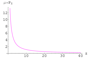
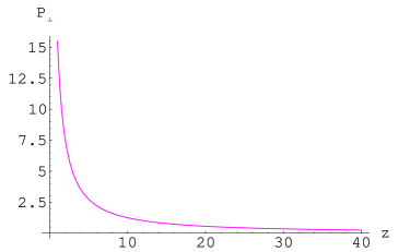
Figure 1: Both graphs have been plotted for $k=2,h_{1}=1$.

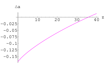
Figure 2: This graph shows that anisotropy increases from negative value to some positive value for $k=2,h_{1}=1$.

3.2 Expansion with $\alpha=\frac{3}{2}$

For expansion, the rate of expansion must be positive, from Eq.(5), $\Theta>0$, when $\alpha\geq 0$, also we assume that

$$B=(z^{2}+{z_{0}}^{2})^{-1}+h_{2}(t),$$ (29)

where $h_{2}(t)$ and $z_{0}$ are arbitrary function and constant respectively.

For $\alpha=\frac{3}{2}$, we get

$$8\pi\mu = 4B-2{B^{-3}}\left[\frac{B^{\prime\prime}}{B}-\left(\frac{B^{\prime}}{B}\right)^{2}\right]+\frac{1}{B^{2}},$$ (30)

$$8\pi P_{z} = 4B+B^{-2}+2B^{-3}\left[\left(\frac{B^{\prime}}{B}\right)^{2}-\frac{\dot{B}^{\prime}}{\dot{B}}\frac{B^{\prime}}{B}\right],$$ (31)

$$8\pi P_{\perp} = -6B+{B^{-3}}\left[-\frac{1}{2}\frac{B^{\prime\prime}}{B}-\frac{7}{2}\frac{\dot{B}^{\prime}}{\dot{B}}\left(\frac{B^{\prime}}{B}\right)+\frac{\dot{B}^{\prime\prime}}{B}+3\left(\frac{B^{\prime}}{B}\right)^{2}\right].$$ (32)

With $F(t,z)=1+h_{2}(t)(z^{2}+{z_{0}}^{2})$ and $B=\frac{F}{(z^{2}+{z_{0}}^{2})}$, the density and pressures in this case are

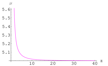
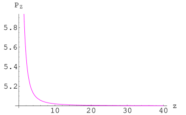
Figure 3: This graph is plotted for $h_{2}=1,z_{0}=1$.

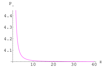
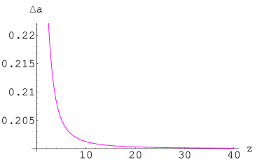
Figure 4: This graph is plotted for $h_{2}=1,z_{0}=1$.

$$8\pi\mu = \frac{4F}{(z^{2}+{z_{0}}^{2})}+\frac{(z^{2}+{z_{0}}^{2})^{2}}{F^{2}}+\frac{(z^{2}+{z_{0}}^{2})({z_{0}}^{2}-3z^{2})}{F^{4}}+\frac{8z^{2}(z^{2}+{z_{0}}^{2})}{F^{5}},$$

$$8\pi P_{z} = \frac{4F}{(z^{2}+{z_{0}}^{2})}+\frac{(z^{2}+{z_{0}}^{2})^{2}}{F^{2}}+\frac{8z^{2}(z^{2}+{z_{0}}^{2})}{F^{5}},$$ (34)

$$8\pi P_{\perp} = \frac{-6F}{(r^{2}+{z_{0}}^{2})}+\frac{(r^{2}+{z_{0}}^{2})({z_{0}}^{2}-3r^{2})}{F^{4}}+\frac{12r^{2}(r^{2}+{z_{0}}^{2})}{F^{5}}.$$ (35)

The dimensionless measure of anisotropy defined by Eq.(6) in this case takes the following form

$$\triangle a=\frac{F^{6}-F(z_{0}^{2}-3{z}^{2})(z^{2}+{z_{0}}^{2})^{2}+\frac{z^{2}(3+8(z^{2}+{z_{0}}^{2})^{2})}{(z^{2}+{z_{0}}^{2})}}{\left(4F^{6}+8z^{2}(z^{2}+{z_{0}}^{2}+F^{3}(z^{2}+{z_{0}}^{2})^{3})\right)}.$$ (36)

All these quantities are shown graphically in figures 3 and 4.

4 Junction Conditions

In this section, we formulate junction conditions for the general spacetime in the interior and vacuum spacetime in the exterior regions, respectively. The quantities in the interior and exterior are denoted by $-$ and $+$, respectively. The line element of the exterior region is (Chao-Guang1995)

$$ds^{2}_{+}=-NdT^{2}+{N}^{-1}dZ^{2}+Z^{2}(dX^{2}+dY^{2}),$$ (37)

where $N(Z)=(\frac{-2M}{Z^{2}})$.

Now using the first junction condition, the continuity of the intrinsic curvature (the first fundamental form)

$$(ds^{2}_{-})_{\Sigma}=(ds^{2}_{+})_{\Sigma},$$ (38)

we have the following equations

$$\frac{dt}{d\tau} = \frac{1}{A},Z_{\Sigma}=B,$$ (39)

$$\frac{dT}{d\tau} = (\frac{-2M}{Z_{\Sigma}})^{\frac{1}{2}}[(\frac{-2M}{Z_{\Sigma}})^{2}-(\frac{dZ_{\Sigma}}{dT})^{2}]^{\frac{-1}{2}},$$ (40)

where $\tau$ is proper time defined for the boundary surface.

The second junction condition is the continuity of the extrinsic curvature (the second fundamental form). The surviving components of the extrinsic curvature for the interior spacetime are found as follows

$$K_{00}^{-} = -[\frac{A^{\prime}}{AC}]_{\Sigma},$$ (41)

$$\ K_{11}^{-} = [\frac{BB^{\prime}}{C}]_{\Sigma}=K_{22}^{-}.$$ (42)

The non-null components of the extrinsic curvature for the exterior spacetime can be found as follows

$$K_{00}^{+} = [\frac{dZ}{d\tau}\frac{d^{2}T}{d\tau^{2}}-\frac{d^{2}Z}{d\tau^{2}}\frac{dT}{d\tau}-\frac{N}{2}\frac{dN}{dZ}(\frac{dT}{d\tau})^{3}+\frac{3}{2N}\frac{dN}{dZ}\frac{dT}{d\tau}(\frac{dZ}{d\tau})^{2}]_{\Sigma}.$$ (43)

$$\ K_{11}^{+} = [ZN\frac{dT}{d\tau}]_{\Sigma}=K_{22}^{+}.$$ (44)

By the continuity of extrinsic curvature components, we have the following two equations

$$-[\frac{A^{\prime}}{AC}]_{\Sigma}=[\frac{dZ}{d\tau}\frac{d^{2}T}{d\tau^{2}}-\frac{d^{2}Z}{d\tau^{2}}\frac{dT}{d\tau}-\frac{N}{2}\frac{dN}{dZ}(\frac{dT}{d\tau})^{3}+\frac{3}{2N}\frac{dN}{dZ}\frac{dT}{d\tau}(\frac{dZ}{d\tau})^{2}]_{\Sigma},$$ (45)

$$[\frac{BB^{\prime}}{C}]_{\Sigma}=[ZN\frac{dT}{d\tau}]_{\Sigma}.$$ (46)

Solving the above equations with Eqs.(39) and (40), we get

$$M\overset{\Sigma}{=}m(t,z).$$ (47)

This is the necessary and sufficient condition for the matching of interior and exterior spacetimes.

5 Conclusion

In this paper, we have studied the generating solution of field equations with anisotropic in plane symmetric geometry. These solutions are only possible due to the null heat flux in the source. The sectional curvature mass as well as trapped surfaces have been studied in detailed. The condition ${B^{\prime}}=B^{2\alpha}$, implies the absence of horizons. Under this condition density becomes decreasing function and fluid maintains its anisotropy, the expansion scalar becomes $\Theta=(2+\alpha)R^{(1-\alpha)}$. This implies that $\Theta=0$, for $\alpha=-2$, $\Theta>0$, for $\alpha\geq 0$, $\Theta<0$, for $\alpha<-2$, which corresponds to bouncing, expansion and collapse, respectively, which corresponds to bouncing, expansion and collapse, respectively. For bouncing all density becomes constant while pressure components are non-zero and zero, which implies that anisotropy remains in the fluid. For collapse the value of $\alpha$ is $\alpha=\frac{-5}{2}$ which implies that $\Theta<0$ and all the matter components and anisotropy are decreasing function of $z$ as shown in figures 1 and 2. To discuss the expansion, we have taken the value $\alpha=\frac{3}{2}$, which implies that $\Theta>0$ and all the matter components and anisotropy are decreasing function of $z$ as shown in figures 3 and 4.

The interior source metric has been matched with the exterior vacuum solution by using the Darmois (1927) junction conditions. The detail analysis of these conditions implies the continuity of interior mass and exterior gravitational mass over the boundary surface.

References

- [1] Bowers, R.L. and Liang, E. P.T.: Astrophys. J. 188, 657(1974)
- [2] Bayin, S.S.: Phys. Rev. D26, 1262(1982)
- [3] Bondi, H.: MNRAS 259, 365(1992)365
- [4] Barcelo, C., Liberati, S., Sonego, S. and Visser, M.: Phys. Rev. D77, 044032(2008)
- [5] Cosenza, M., Herrera, L., Esculpi, M. and Witten, L.: J. Math. Phys. 22, 118(1981)
- [6] Cognola, G., Elizalde, E., Nojiri, S, Odintov, S.D. and Zerbini, S.: Phys. Rev. D75, 086002(2007)
- [7] Chao-Guang, H.: Acta Physica Sinica 4, 617(1995)
- [8] Darmois, G.: Memorial des Sciences Mathematiques (Gautheir-Villars, Paris, 1927)
- [9] Glass, E.N.: Phys. Lett. A86, 351(1981)
- [10] Glass, E.N.: Gen. Relativ. Gravit. 45, 2661(2013)
- [11] Gasperini, M. and Veneziano, G.: Astropart. Phys. 1, 317(1993)
- [12] Herrera, L., Ospino, J. and Di Prisco, A.: Phys. Rev. D77, 027502(2008a)
- [13] Herrera, L. and Santos, N.O.: Phys. Rep. 286, 53(1997)
- [14] Herrera, L., Santos, N.O. and Wang, A.: Phys. Rev. D78, 084024(2008b)
- [15] Misner, C.W., Sharp, D.: Phys. Rev. 136, B571(1964)
- [16] Misner C.W. and Sharp, D.H.: Phys. Lett. 15, 279(1965)
- [17] Nojiri, S. and Odintov, S.D.: Phys. Lett. B631, 1(2005)
- [18] Nojiri, S., Odintov S.D. and Gorbunova, O.G.: J. Phys. A39, 6627(2006)
- [19] Oppenheimer, J.R., Snyder, H.: Phys. Rev. 56, 455(1939)
- [20] Sharif, M. and Zaeem, M.: Mod. Phys. Lett. A27, 1250141(2012)
- [21] Sharif, M. and Yousaf, Z.: Can. J. Phys. 90, 865(2012)
- [22] Sharif, M. and Abbas, G.: J. Phys. Soc. Jpn. 82, 034006(2013)
- [23] Zannias, T.: Phys. Rev. D41, 3252(1990).
- [24]