Constraining Sub-Parsec Binary Supermassive Black Holes in Quasars with Multi-Epoch Spectroscopy. II. The Population with Kinematically Offset Broad Balmer Emission Lines

Abstract

A small fraction of quasars have long been known to show bulk velocity offsets (of a few hundred to thousands of km s^-1) in the broad Balmer lines with respect to the systemic redshift of the host galaxy. Models to explain these offsets usually invoke broad-line region gas kinematics/asymmetry around single black holes (BHs), orbital motion of massive ($\sim$sub-parsec (sub-pc)) binary black holes (BBHs), or recoil BHs, but single-epoch spectra are unable to distinguish between these scenarios. The line-of-sight (LOS) radial velocity (RV) shifts from long-term spectroscopic monitoring can be used to test the BBH hypothesis. We have selected a sample of 399 quasars with kinematically offset broad H$\beta$ lines from the Sloan Digital Sky Survey (SDSS) Seventh Data Release quasar catalog, and have conducted second-epoch optical spectroscopy for 50 of them. Combined with the existing SDSS spectra, the new observations enable us to constrain the LOS RV shifts of broad H$\beta$ lines with a rest-frame baseline of a few years to nearly a decade. While previous work focused on objects with extreme velocity offset ($>10^{3}$ km s^-1), we explore the parameter space with smaller (a few hundred km s^-1) yet significant offsets (99.7% confidence). Using cross-correlation analysis, we detect significant (99% confidence) radial accelerations in the broad H$\beta$ lines in 24 of the 50 objects, of $\sim$10–$200$ km s^-1 yr^-1 with a median measurement uncertainty of $\sim$10 km s^-1 yr^-1, implying a high fraction of variability of the broad-line velocity on multi-year timescales. We suggest that 9 of the 24 detections are sub-pc BBH candidates, which show consistent velocity shifts independently measured from a second broad line (either H$\alpha$ or Mg II) without significant changes in the broad-line profiles. Combining the results on the general quasar population studied in Paper I, we find a tentative anti-correlation between the velocity offset in the first-epoch spectrum and the average acceleration between two epochs, which could be explained by orbital phase modulation when the time separation between two epochs is a non-negligible fraction of the orbital period of the motion causing the line displacement. We discuss the implications of our results for the identification of sub-pc BBH candidates in offset-line quasars and for the constraints on their frequency and orbital parameters.

1. Introduction

This paper describes a search for temporal radial velocity (RV) shifts (i.e., accelerations) of quasar broad emission lines as evidence for massive, sub-parsec (sub-pc) binary black holes (BBHs). Our working hypothesis is that only one of the two BHs in the binary is active and powering its own broad-line region (BLR), and that the binary separation is sufficiently large compared to the BLR size that the broad line velocity traces the binary motion, yet small enough that the acceleration can be detected over the temporal baseline of our observations. In Shen et al. (2013, hereafter Paper I), we have reported results for the general quasar population. Here, in the second paper of this series, we target a sample of quasars with offset broad Balmer emission lines, to probe a different and complementary parameter space. To date, no convincing case of a sub-pc BBH has been found.

1.1. Motivation to Search for Sub-pc BBHs

Theoretical models for the observed evolution of galaxies and BHs suggest that BBHs should be common (Begelman et al., 1980; Roos, 1981; Milosavljević & Merritt, 2001; Yu, 2002; Colpi & Dotti, 2011; Merritt, 2013). are expected to be the most abundant at binary separations between $\sim 1$ pc and $\sim 10^{-3}$ pc, where the orbital decay has slowed due to loss cone depletion (e.g., Begelman et al., 1980; Gould & Rix, 2000), and the emission of gravitational waves (GWs) is not yet efficient (Thorne & Braginskii, 1976; Centrella et al., 2010). Whether or not the BBH orbit enters the GW regime, and the relative importance of gas and stellar dynamical processes in facilitating such decays, are still subject to active debate (e.g., Gould & Rix, 2000; Escala et al., 2005; Merritt & Milosavljević, 2005; Mayer et al., 2007; Dotti et al., 2012; Vasiliev et al., 2014). A determination of the frequency of sub-pc BBHs would help constrain the orbital decay rate and inform the expected abundance of low-frequency GW sources (e.g., Sesana, 2007; Trias & Sintes, 2008; Amaro-Seoane et al., 2012). It would also test models of BH assembly and growth in hierarchical cosmologies (e.g., Volonteri et al., 2009; Kulkarni & Loeb, 2012).

1.2. Evidence for Massive BH Pairs on Various Scales

Merger models have been successful in reproducing the observed demographics and spatial distribution of galaxies and quasars across cosmic time (e.g., Kauffmann & Haehnelt, 2000; Volonteri et al., 2003; Wyithe & Loeb, 2003; Hopkins et al., 2008; Shen, 2009). At wide separations, from tens of kpc to $\sim$kpc scales, there is strong direct evidence for active BH pairs in merging or merged galaxies (e.g., Komossa et al., 2003; Ballo et al., 2004; Bianchi et al., 2008; Comerford et al., 2009, 2011, 2012; Wang et al., 2009; Smith et al., 2010; Green et al., 2010; Liu et al., 2010b, a, 2011b, 2011a, 2013; Shen et al., 2011a, 2010; Piconcelli et al., 2010; Fabbiano et al., 2011; Fu et al., 2012, 2011; Greene et al., 2011; Koss et al., 2011, 2012; Mazzarella et al., 2012; McGurk et al., 2011); their observed frequency can be reasonably well explained by merger models (Yu et al., 2011; Van Wassenhove et al., 2012).

At $\sim$pc to sub-pc separations, however, CSO 0402+379 remains the only secure case known: this is a compact flat-spectrum double radio source (Rodriguez et al., 2006) serendipitously discovered by the Very Long Baseline Array, with a projected separation of $\sim 7$ pc. While sub-pc BBHs are largely elusive, there is indirect evidence, at least in local massive elliptical galaxies, that they may have had a strong dynamical impact on the stellar structures at the centers of galaxies by scouring out flat cores (e.g., Ebisuzaki et al., 1991; Faber et al., 1997; Graham, 2004; Kormendy et al., 2009; Merritt, 2013).

Sub-pc BBHs may be abundant but either mostly inactive or just difficult to resolve. Direct imaging searches in the radio have proven extremely challenging (e.g., Burke-Spolaor, 2011), largely because of both insufficient resolving power (even the unparalleled resolution of the very long baseline interferometry can only resolve very nearby sources, e.g., $z<0.01$ for $\sim$pc or $z<0.001$ for $\sim 0.1$pc separations) and the small probability for both BHs to be simultaneously bright in the radio. On the other hand, the dynamical signature of binary orbital motion, in principle, can be used to identify candidate sub-pc BBHs (e.g., Komberg, 1968; Gaskell, 1983; Loeb, 2010; Shen & Loeb, 2010; Eracleous et al., 2012; Popović, 2012), in analogy to spectroscopic binary stars (e.g., Abt & Levy, 1976). In particular, it has long been proposed that BBH candidates may be selected from quasars whose broad emission lines are offset from the systemic velocities of their host galaxies (e.g., Gaskell, 1983; Peterson et al., 1987; Halpern & Filippenko, 1988; Bogdanović et al., 2009). Large spectroscopic surveys have enabled the selection of statistical samples of quasars with offset broad lines (Bonning et al., 2007; Boroson & Lauer, 2010; Shen et al., 2011b; Tsalmantza et al., 2011; Eracleous et al., 2012), as well as individual interesting cases (e.g., Boroson & Lauer, 2009; Shields et al., 2009).

However, there are alternative, and perhaps more natural, explanations for broad-line velocity offsets, such as gas motion in the accretion disk around a single BH (so-called “disk emitters”; e.g., Chen et al., 1989; Eracleous et al., 1995; Shapovalova et al., 2001; Eracleous & Halpern, 2003; Strateva et al., 2003). Single-peaked but offset broad emission lines may be disks with high emissivity asymmetry or the other peak may be too weak to identify (e.g., Chornock et al., 2010). Yet another scenario is a recoiled BH (e.g., Campanelli et al., 2007; Bonning et al., 2007; Loeb, 2007; Shields et al., 2009) from the anisotropic GW emission following BBH coalescence (e.g., Fitchett, 1983; Baker et al., 2006), which carries the inner part of its accretion disk and a BLR with it, and could fuel a continuing quasar phase for millions of years (e.g., Loeb, 2007; Blecha et al., 2011). The recoil scenario is perhaps less likely for offsets $\gtrsim$ a few hundred km s^-1 (e.g., Bogdanović et al., 2007; Dotti et al., 2010), since recoil velocities tend to be smaller than this when the BH spin axes are aligned, which tends to happen in gas-rich mergers. Another mechanism for even larger kicks is slingshot ejection of a BH from a triple system, formed when a new galaxy merger occurs before a pre-existing BBH has coalesced (Hoffman & Loeb, 2007; Kulkarni & Loeb, 2012).

1.3. Summary of Previous Radial Velocity Monitoring

The temporal RV shift of broad emission lines offers a promising test for the BBH hypothesis (e.g., Eracleous et al., 1997; Shen & Loeb, 2010). Dedicated long-term (i.e., more than a few years) spectroscopic monitoring programs are needed, as the binary orbital periods are typically several decades to several centuries (e.g., Yu, 2002; Loeb, 2010). Depending on properties of the broad emission lines in single-epoch spectra, there are the following strategies for looking for BBHs using temporal RV shifts:

1. monitor quasars with double-peaked broad lines (which, by definition, usually show extreme (i.e., $>$ a few thousand km s^-1) offset velocities in both peaks);

2. monitor quasars having single-peaked broad lines with significant velocity offsets;

3. monitor the much larger population of quasars having single-peaked broad lines without offsets.

Most earlier spectroscopic monitoring work has focused on quasars with double-peaked broad lines, most notably 3C 390.3 (Gaskell, 1996; Eracleous et al., 1997; Shapovalova et al., 2001), Arp 102B (Halpern & Filippenko, 1988), NGC 5548 (Peterson et al., 1987; Shapovalova et al., 2004; Sergeev et al., 2007), and NGC 4151 (Shapovalova et al., 2010; Bon et al., 2012). Long-term spectroscopic monitoring studies of quasars with double-peaked broad lines suggest that most of them are likely explained by emission from gas in the outer accretion disk rather than BBHs (e.g., Halpern & Filippenko, 1988; Eracleous, 1999; Eracleous & Halpern, 2003). The long-term line profile/velocity changes in such objects are likely caused by transient dynamical processes (e.g., shocks from tidal perturbations) or physical changes (e.g., emissivity variation and/or precession of fragmented spiral arms) in the line emitting region in the outer accretion disk around single BHs (Gezari et al., 2007; Lewis et al., 2010). Furthermore, there are reasons to expect that most BBHs do not exhibit double-peaked broad lines, because there is limited parameter space, if any, for two well-separated broad-line peaks to be associated with two physically distinct BLRs (e.g., Shen & Loeb, 2010).

While double-peaked broad lines are likely not a promising diagnostic to look for BBHs, the case remains open for single-peaked broad-line offsets. In principle, the probability of having one BH active is much higher than having both BHs simultaneously active, and the allowed binary parameter space is also larger than in the case with double-peaked broad lines. Recently Eracleous et al. (2012) carried out the first systematic spectroscopic followup study of quasars with offset broad H$\beta$ lines. The authors identified 88 quasars with broad-line offset velocities of $\gtrsim 10^{3}$ km s^-1 and conducted second-epoch spectroscopy of 68 objects. They found significant (at 99% confidence) velocity shifts in 14 objects, with accelerations in the range of [$-120$, 120] km s^-1 yr^-1. Decarli et al. (2013) also obtained second-epoch spectra for 32 Sloan Digital Sky Survey (SDSS; York et al., 2000) quasars selected to have peculiar broad-line profiles (Tsalmantza et al., 2011), such as large velocity offsets ($\gtrsim 1000$ km s^-1) and/or double-peaked or asymmetric line profiles. However, the conclusions from Decarli et al. (2013) are relatively weak, as they measured velocity shifts using model fits to the emission-line profiles rather than the more powerful cross-correlation approach adopted by Eracleous et al. (2012), Paper I, and this work. Nevertheless, at least for BBH candidates with symmetric line profiles, the line fitting method should still be a sensible (albeit less sensitive) tool to look for velocity shifts.

Finally, for the general quasar population (i.e., without broad-line offsets), Paper I presents the first statistical spectroscopic monitoring study based on the broad H$\beta$ lines (see also Ju et al., 2013, for a similar study but based on Mg II $\lambda$2800).

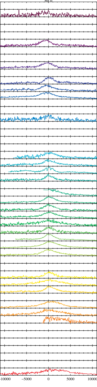
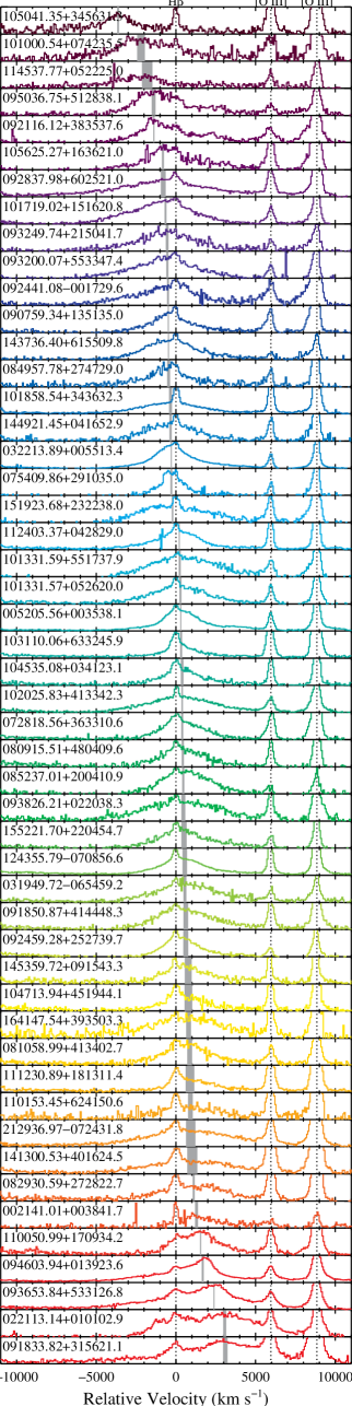
Figure 1.— Examples of quasars with offset broad Balmer emission lines. Spectra are shown in arbitrarily normalized flux density, in the Mg II $\lambda$2800 (left column), H$\beta$ (middle column), and H$\alpha$ (right column) region. Objects are ordered according to broad H$\beta$ peak velocity offsets, as indicated by the gray shaded areas (with 1 $\sigma$ uncertainties). Wavelength scales are in relative velocity centered on the systemic velocity. Labels in the middle column are SDSS designations with R.A. and decl. for each object.

1.4. This Work

We have compiled a large sample (399 objects) of significantly (99.7% confidence) offset broad-line quasars (see also Shen et al., 2011b). They were selected from the quasar catalog (Schneider et al., 2010) in the Seventh Data Release (DR7; Abazajian et al., 2009) of the SDSS. Their broad H$\beta$ lines (as well as H$\alpha$ or Mg II, when available) show significant velocity offsets of $\gtrsim$ a few hundred km s^-1 relative to the systemic redshift determined from narrow emission lines (Section 2). To mitigate contamination by disk emitters, we focus on objects with well-defined single-peaked offset broad lines. As a pilot program, we have obtained a second-epoch optical spectrum, separated by $\sim$5–10 yr (rest frame) from the original SDSS spectrum, for a subset of 50 objects in the sample (Section 3). We measure the temporal velocity shifts of the broad emission lines (Section 5) using a cross-correlation method (Section 4) to constrain the BBH hypothesis and model parameters (Section 6). We have detected significant (99% confidence) shifts in 24 objects (Section 5.4), of which we suggest that 9 are strong BBH candidates (Section 5.4.1), and future observations can definitively test this suggestion. Our results have implications for the general approach of identifying BBH candidates in offset-broad-line quasars, for the orbital evolution of sub-pc BBHs, and for the forecast of low-frequency GW sources (Section 6).

Our program has two major differences from previous work. First, we probe a parameter space in broad-line velocity offset that is complementary to both the general quasar population studied in Paper I and the population with more extreme offset velocities examined in other statistical studies (Eracleous et al., 2012; Decarli et al., 2013). Therefore by selection our sample would probe a different parameter space in the BBH scenario, since the velocity offset is determined by BH masses, binary separations, orbital phases, and inclinations (e.g., the Appendix). Second, in contrast to previous studies on offset-line quasars which often adopt some minimum threshold on the measured offset velocity, we apply the threshold on the statistical significance of the measured offset velocity (where the measurement uncertainty depends on signal-to-noise ratio (S/N) of the spectrum and on line widths; Paper I). As a result, our sample includes small but significant velocity offsets. Combined with the results of Paper I, the improved statistics and the enlarged dynamic range enable us to study the statistical relation between velocity offset and acceleration (Section 5.3), to examine whether the observations are consistent with the BBH hypothesis. Understanding the origin of the broad-line velocity offsets in single-epoch spectra is important for addressing the selection biases of offset-line quasars to put their monitoring results in the context of the general population.

Throughout this paper, we assume a concordance cosmology with $\Omega_{m}=0.3$, $\Omega_{\Lambda}=0.7$, and $H_{0}=70$ km s^-1 Mpc^-1, and use the AB magnitude system (Oke, 1974). Following Paper I, we adopt “offset” to refer to the velocity difference between two lines in single-epoch spectra, and “shift” to denote changes in the line velocity between two epochs. We quote velocity offsets relative to the observer, i.e., negative values mean blueshifts. We define accelerations relative to the original SDSS observations, where positive means moving toward longer wavelengths. All time intervals and relative velocities are in the quasar rest frames by default, unless noted otherwise.

2. SDSS Quasars with Offset Broad Balmer Emission Lines

A fraction of quasars have long been noticed to have bulk velocity offsets (both blueshifts and redshifts with absolute velocities $\sim$a few hundred to thousand km s^-1) in the broad permitted emission lines (e.g., H$\beta$ and H$\alpha$) with respect to the systemic velocity (determined from narrow emission lines and/or stellar absorption features) of the host galaxies (e.g., Osterbrock & Shuder, 1982). Quasars with offset broad lines are rare ($\sim$a few percent, depending on offset velocity; e.g., Bonning et al., 2007), but large spectroscopic redshift surveys such as the SDSS have increased the inventory of such objects by orders of magnitude (e.g., Boroson & Lauer, 2010; Shen et al., 2011b; Tsalmantza et al., 2011). In this section, we first describe the selection and general properties of a sample of SDSS quasars with offset broad Balmer emission lines (Section 2.1). We then discuss selection biases and uncertainties (Section 2.2).

2.1. Sample Selection

We start with the SDSS DR7 quasar catalog (Schneider et al., 2010), adopting the spectral measurements of Shen et al. (2011b). The catalog contains 105,783 spectroscopically confirmed quasars at redshifts $0.065<z<5.46$. These quasars have luminosities $M_{i}<-22.0$ and at least one broad emission line with FWHM larger than 1000 km s^-1. The SDSS DR7 provides optical spectra covering $\lambda=3800$–9180 Å with moderate spectral resolution ($R\sim 1850$–2200) and S/N ($\sim$ 15 pixel^-1, with the pixel size being $69$ km ${\rm s}^{-1}$). Among the SDSS DR7 quasars, 20,774 are at $z<0.83$, where SDSS spectra cover H$\beta$ and [O III] $\lambda\lambda$4959,5007 (hereafter [O III] for short). As we discuss in detail below, from this parent sample of 20,774 objects we select a subset of 399 with offset broad Balmer emission lines, based on the spectral region around H$\beta$ and [O III]. Our selection was a combination of automated spectral fitting (Shen et al., 2008, 2011b) and visual examination. Here and throughout, we refer to the 399 objects as the “offset” sample. Below, we first briefly describe the spectral model fitting (Section 2.1.1). We refer to Shen et al. (2011b) and Paper I for details. We then discuss the selection procedure in Sections 2.1.2–2.1.4 and discuss the properties of the samples in Section 2.1.5.

2.1.1 Spectral Model Fitting

To measure velocity offsets between the broad and narrow emission lines, we first construct models of the spectra. Each SDSS spectrum was decomposed using a combination of models for the power-law continuum, Fe II emission complex, broad emission lines, and narrow emission lines. First, the line-less regions are fit by a pseudo-continuum model using an Fe II template plus a power-law continuum. After subtracting the pseudo-continuum, the narrow and broad emission lines are then fit using multiple Gaussians, where the widths and mean velocities of different narrow lines are constrained to be the same. The fitting was performed separately around each broad emission line (H$\alpha$, H$\beta$, and Mg II). For the H$\beta$ region, [O III] is occasionally fit by two Gaussians for the core and wing (possibly associated with narrow-line region outflows) components. In these cases, the width and mean velocity of the narrow H$\beta$ emission line are constrained to be the same as those of the core [O III] component. All fits have been checked by visual inspection to ensure that models reproduce data well.

2.1.2 Measuring Velocity Offsets of Broad Emission Lines

Using the spectral models, we measure the offset of the broad emission lines relative to the systemic velocity. The systemic redshift is estimated from the core component of [O III], which may be different (by a median offset of $32$ km s^-1 with a standard deviation of $125$ km s^-1) from the nominal redshift listed by the DR7 catalog based on the SDSS spectroscopic pipeline (Stoughton et al., 2002). Our adopted systemic redshift agrees with the improved redshift for SDSS quasars from Hewett & Wild (2010) within uncertainties. As discussed in Paper I, we focus on the H$\beta$–[O III] region. [O III] allows a good estimate of the systemic redshift, and also provides empirical constraints on the profile of the narrow H$\beta$ component. While H$\alpha$ is stronger than H$\beta$ and therefore offers better S/N for each object, it would restrict us to a $\sim$five times smaller parent sample (i.e., 3873 quasars in total at $z<0.36$). Compared to H$\beta$, C IV and Mg II are less well understood in terms of their BLR structure; furthermore, C IV is more asymmetric and more likely to be associated with a non-virial outflowing component. Despite these caveats, we also compare H$\beta$ with independent measurements from Mg II and H$\alpha$ when available to control systematics and check for consistency.

2.1.3 Automatic Pipeline Selection

We first examine whether there is a significant (99.7% confidence) velocity offset in broad H$\beta$ relative to the systemic redshift using the spectral model from automatic pipeline fitting. Our selection criteria are the following:

1. Median S/N pixel^-1 $>5$ in rest-frame 4750–4950 Å.

2. Broad H$\beta$ rest-frame equivalent width $>3\sigma_{{\rm EW}}$.

3. $|V_{{\rm off}}|>3\sigma_{V_{{\rm off}}}$, where $\sigma_{V_{{\rm off}}}$ is the total velocity offset error propagated from the velocity uncertainties of both broad and narrow emission lines.

The uncertainty of the velocity offset, $\sigma_{V_{{\rm off}}}$, taking into account both photon noise in the spectrum and the ambiguity in subtracting a narrow-line component, was estimated from Monte Carlo simulations (Shen et al., 2011b).

We have experimented with two measures of the velocity offset $V_{{\rm off}}$ of the broad emission line with respect to the systemic redshift: the line centroid and line peak. These two measures generally give consistent results for objects whose broad-line profile is well-fit by a single Gaussian. But for objects with more complex broad-line profiles, which are usually well-fit by multiple Gaussians, the two measures can give different results. We demand that $|V_{{\rm off}}|>3\sigma_{V_{{\rm off}}}$ for both the line centroid and the line peak. The automatic selection yielded 1212 objects with measurable velocity offsets in the broad H$\beta$ out of the 20,574 objects.

Figure 2.— Distribution of quasar properties (redshift, bolometric luminosity, virial BH mass estimate, and BLR size) for the parent, offset, followup, and velocity-shift detected sample. Labeled on each panel are median values for different samples.

2.1.4 Visual Inspection

We then visually inspected all the 1212 objects to verify the pipeline measurements. We removed unreliable fits caused by noise, weak broad H$\beta$ components, inconsistent results in H$\alpha$ or Mg II, and/or problematic systemic redshift due to weak, broad, winged and/or double-peaked [O III] without a reliable narrow H$\beta$; we rejected narrow-line Seyfert 1 galaxies (with broad H$\beta$ FWHM $<2000$ km s^-1, the ratio of [O III] $\lambda$5007 to H$\beta$ smaller than three, and strong optical Fe II emission; e.g., Osterbrock & Pogge, 1985; Goodrich, 1989) whose broad H$\beta$ often have blue wings (e.g., Boroson & Green, 1992), which may be attributed to outflowing gas in the H$\beta$ emitting part of the BLR around small BHs with high Eddington ratios (e.g., Boroson, 2002); we also rejected objects with prominent double-peaked broad emission lines, which are most likely due to accretion disk emission around single BHs as discussed above. This visual inspection yielded 399 objects, which constitute our final “offset” sample. We present the full offset sample in Table 1 with basic measurements. Figure 1 shows SDSS spectra of 50 examples from the offset sample.

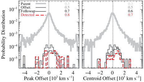
Figure 3.— Distribution of broad H$\beta$ velocity offset for the parent, offset, followup, and velocity-shift detected sample. The left panel shows the peak velocity and the right panel shows the centroid. Labeled on the plot are median values (in units of $10^{3}$ km s^-1) of $|V_{{\rm off}}-V^{0}_{{\rm off}}|$ for different samples, where $V^{0}_{{\rm off}}$ denotes median values of $V_{{\rm off}}$. Vertical dotted lines indicate $V^{0}_{{\rm off}}$ for the parent sample (which is consistent with zero for the peak velocity, or $80\pm 6$ km s^-1 for the centroid velocity).

2.1.5 Sample Properties

Figure 2 shows the basic quasar properties (redshift, luminosity, virial BH mass, and BLR size) for the parent sample and the offset sample. The bolometric luminosity and virial BH mass estimates (e.g., Shen, 2013) were taken from Shen et al. (2011b). The BLR sizes $R$ were estimated from the 5100 Å continuum luminosity assuming the empirical $R$–$L_{5100}$ relation in Bentz et al. (2009). The quasar luminosity distribution of the offset sample is similar to the parent sample, whereas the redshift is lower than that of the parent sample (median redshift of 0.42 and 0.55, respectively). The estimated virial BH masses and BLR sizes of the offset sample are both similar to those of the parent quasar sample.

Figure 3 shows broad H$\beta$ peak and centroid velocity offsets for the parent and offset samples. By construction, the offset sample has larger $|V_{{\rm off}}|$ than the parent sample (median value of $\sim 500$ km s^-1 compared to $\sim 300$ km s^-1). The offset sample also has larger broad H$\beta$ emission line offsets relative to the general quasar population studied in Paper I: most of our offset objects have $300<|V_{{\rm off}}|<1000$ km s^-1, whereas most ordinary quasars have $|V_{{\rm off}}|<300$ km s^-1. By comparison, the majority of the Eracleous et al. (2012) sample has peak $|V_{{\rm off}}|>1000$ km s^-1.

For the parent sample the velocity centroid offset distribution is centered at $80\pm 6$ km s^-1, likely due to gravitational redshift and transverse Doppler shift in BLR clouds close to the BH (e.g., Zheng & Sulentic, 1990; Corbin & Boroson, 1996; Tremaine et al., 2014). For the offset sample the observed velocity peak and centroid offset distributions are centered around $\sim 200\pm 40$ km s^-1, i.e., redshifted relative to the systemic velocity. Subtracting the $80\pm 6$ km s^-1 measured from the parent sample (assuming it is due to gravitational redshift and transverse Doppler shift), the corrected distribution center is $\sim 120\pm 40$ km s^-1. This residual redshift is likely a selection bias, caused by our rejection of broad H$\beta$ blue wings (Section 2.1.4). The rejection was meant to eliminate narrow-line Seyfert 1s, but objects with small blue velocity offsets (i.e., $\sim 100$ km s^-1) may be mistaken for blue wings and got rejected more often than those with small red offsets.

Figure 4.— Distribution of broad H$\beta$ FWHMs and median S/N pixel^-1 of the SDSS spectra for the parent, offset, followup, and velocity-shift detected sample. The median values for different samples are indicated.

Table 1SDSS Quasars with Kinematically Offset Broad Balmer Emission Lines

SDSS Designation	$z_{{\rm sys}}$	Plate	Fiber	MJD	$V^{{\rm peak}}_{{\rm off}}$	$\sigma_{V_{{\rm off}}}$	$V^{{\rm cen}}_{{\rm off}}$
(1)	(2)	(3)	(4)	(5)	(6)	(7)	(8)
001224.01$-$102226.5	0.2288	0651	072	52141	$-$1952	119	$-$638
001247.93$-$084700.5	0.2203	0652	326	52138	$-$176	39	283
001257.25+011527.3	0.5047	0389	379	51795	717	162	753
002043.58+141249.4	0.5880	0753	253	52233	379	65	375

Note. — Column 1: SDSS names with J2000 coordinates given in the form of “hhmmss.ss+ddmmss.s”; Column 2: systemic redshift from Hewett & Wild (2010); Columns 3–5: Plate ID, fiber ID, and MJD of the SDSS spectrum; Column 6: broad H$\beta$ peak velocity offset in km s^-1. Positive (negative) value means redshift (blueshift); Column 7: 1$\sigma$ uncertainty of broad H$\beta$ peak velocity offset in km s^-1, taking into account both statistical and systematic errors estimated from Monte Carlo simulations (Shen et al., 2011b); Column 8: broad H$\beta$ centroid velocity offset in km s^-1.

(This table is available in its entirety in a machine-readable form in the online journal. A portion is shown here for guidance regarding its form and content.)

2.2. Selection Biases and Incompleteness

We discuss possible selection biases to put our offset quasar sample into the context of the general quasar population. First, the visual inspection is subjective and by no means complete, and the resulting bias cannot be easily quantified. Second, only about half of the objects in the parent quasar catalog were selected uniformly using the final quasar target selection algorithm (Richards et al., 2002); the remaining objects were selected via earlier algorithms or serendipitously (Schneider et al., 2010), and in this case the selection function cannot be easily quantified. Nevertheless, we do not believe that any of our results depend significantly on these complications in the selection function.

Third, the S/N threshold of our automatic selection is somewhat arbitrary and may bias against less luminous quasars. Nevertheless, the effect is mainly on redshift and not on quasar luminosity (Figure 2). However, the parent quasar catalog was defined to have $M_{i}<-22.0$, so that the offset sample is inherently more incomplete at lower luminosities and by extension lower masses. This may be an important bias considering that the figure of merit of detecting BBHs may depend on quasar luminosity (Paper I).

Figure 4 shows the broad H$\beta$ line widths and S/N measured from the SDSS spectra. The median broad H$\beta$ FWHM of the offset sample is $\sim 10$% smaller than that of the parent quasar sample. The median S/N of the offset sample is $\sim 60$% higher than that of the parent quasar sample. As shown in Paper I, the measurement errors in the velocity shift of broad emission lines increase with increasing line width and decreasing S/N. These uncertainties would cause different sensitivities in the measured velocity shifts. We will return to uncertainties in the velocity shift measurement in Section 4.2.

Finally, for BBHs in quasars, by selection objects with offset broad lines may be different from the general population in terms of binary separation, orbital phase, inclination, and BH mass. The resulting effects must be properly accounted for to translate the detection rate into constraints on the binary fraction in the general quasar population. In Section 5.3 we discuss these possible effects in the context of detecting BBH candidates.

Table 2Followup Spectroscopy of SDSS Quasars with Offset Broad Balmer Emission Lines

		$r$			$t_{{\rm exp}}$	S/N	$\Delta t$	$V_{{\rm ccf}}$	$a_{{\rm ccf}}$
No.	SDSS Designation	(mag)	Spec	UT	(s)	(pixel-1)	(yr)	(km s-1)	(km s-1 yr-1)	Category
(1)	(2)	(3)	(4)	(5)	(6)	(7)	(8)	(9)	(10)	(11)
01	001224.02$-$102226.5	16.97	BCS	110731	1200	16	8.31	$-193^{+55}_{-51}$	$-23^{+7}_{-6}$	2
02	001257.25$+$011527.3	18.78	BCS	111227	2400	10	7.70	$-213^{+90}_{-89}$	$-27^{+11}_{-12}$	3
03	002141.02$+$003841.7	18.65	FAST	120126	9000	5	8.70	$-103^{+205}_{-221}$	$-11^{+22}_{-26}$	$\cdots$
04	004712.58$-$084330.8	18.53	BCS	111227	1200	13	7.33	$131^{+53}_{-50}$	$17^{+8}_{-6}$	3
05	011110.04$-$101631.8	16.74	BCS	111227	1200	35	8.87	$27^{+63}_{-55}$	$3^{+7}_{-6}$	$\cdots$
06	014219.00$+$132746.6	18.12	FAST	111129	16200	14	9.03	$-379^{+146}_{-139}$	$-42^{+17}_{-15}$	3
07	020011.53$-$093126.2	18.02	BCS	111226	2400	5	7.79	$365^{+442}_{-563}$	$46^{+57}_{-71}$	$\cdots$
08	022113.14$+$010102.9	18.15	BCS	111227	3600	3	8.41	$179^{+277}_{-548}$	$21^{+33}_{-64}$	$\cdots$
09	032838.28$-$000341.7	19.21	BCS	111227	1200	16	6.44	$-627^{+67}_{-69}$	$-97^{+10}_{-11}$	3
10	073915.36$+$401445.7	18.41	FAST	120126	18000	7	8.84	$206^{+283}_{-313}$	$23^{+32}_{-35}$	$\cdots$
11	074541.67$+$314256.7	15.81	FAST	120103	1800	15	7.10	$117^{+174}_{-180}$	$16^{+25}_{-24}$	$\cdots$
12	080202.79$+$101943.1	18.18	FAST	120127	18000	17	4.23	$6^{+56}_{-57}$	$1\pm 13$	$\cdots$
13	081032.73$+$565105.3	18.92	FAST	120103	18000	16	5.60	$41^{+103}_{-108}$	$7^{+18}_{-19}$	$\cdots$
14	082930.60$+$272822.7	18.10	FAST	111104	25200	23	6.24	$-213^{+129}_{-127}$	$-34^{+21}_{-20}$	1
15*	084716.04$+$373218.1	18.45	DIS	100416	2700	17	5.76	$55^{+46}_{-39}$	$10^{+8}_{-7}$	1
16	085237.02$+$200411.0	18.10	DIS	100416	2700	17	3.12	$-296^{+162}_{-120}$	$-95^{+52}_{-38}$	1
17	091833.82$+$315621.2	17.94	DIS	100416	3600	28	4.47	$738^{+110}_{-102}$	$165^{+24}_{-23}$	3
18${\dagger}$	091858.15$+$232555.4	17.60	FAST	120130	16200	2	3.70	$-41^{+564}_{-571}$	$-11^{+130}_{-154}$	$\cdots$
19	091930.32$+$110854.0	17.25	FAST	111228	18000	22	5.89	$82^{+185}_{-154}$	$14^{+31}_{-26}$	$\cdots$
20${\dagger}$*	091941.13$+$534551.4	18.82	DIS	100416	3600	11	5.94	$204^{+132}_{-99}$	$59^{+22}_{-17}$	3
21	092837.98$+$602521.0	17.01	FAST	120313	5400	25	8.87	$220^{+154}_{-207}$	$24^{+18}_{-23}$	1
22	093653.84$+$533126.8	16.88	FAST	111130	19800	40	8.26	$-303^{+75}_{-81}$	$-36^{+9}_{-10}$	2
23	101000.54$+$074235.5	18.99	FAST	111229	18000	15	6.01	$165^{+74}_{-85}$	$27^{+12}_{-14}$	3
24	102106.05$+$452331.9	18.34	DIS	110601	3600	22	6.38	$0^{+95}_{-89}$	$0\pm 14$	$\cdots$
25	103059.09$+$310255.8	16.77	FAST	120119	1800	13	5.97	$289^{+130}_{-133}$	$48\pm 22$	1
26	104448.81$+$073928.6	18.31	FAST	120101	14400	22	7.50	$689^{+156}_{-124}$	$92^{+19}_{-17}$	2
27	110051.02$+$170934.3	18.48	DIS	110601	3600	21	3.20	$-269^{+92}_{-94}$	$-84\pm 29$	1
28	111230.90$+$181311.4	18.13	FAST	120101	9000	17	4.10	$-124^{+88}_{-86}$	$-30^{+22}_{-21}$	1
29	112007.43$+$423551.4	17.31	FAST	120119	18000	31	6.60	$-89^{+71}_{-74}$	$-13\pm 11$	2
30	113640.91$+$573840.0	17.33	FAST	120129	9000	10	7.81	$-138^{+208}_{-249}$	$-17^{+26}_{-32}$	$\cdots$
31	115449.42$+$013443.5	17.89	DIS	100416	2700	13	6.22	$-96^{+188}_{-317}$	$-15^{+29}_{-51}$	$\cdots$
32	122018.44$+$064119.6	17.51	FAST	120313	5400	16	5.52	$731^{+66}_{-921}$	$132^{+12}_{-166}$	$\cdots$
33${\ddagger}$	122811.89$+$514622.8	18.43	DIS	110601	4500	16	7.10	$-13^{+62}_{-63}$	$-1^{+7}_{-9}$	$\cdots$
34*	130534.49$+$181932.9	16.68	DIS	100412	2700	24	1.98	$236^{+79}_{-76}$	$119\pm 39$	1
35	130712.34$+$340622.5	17.51	FAST	120419	5400	15	6.27	$172^{+143}_{-144}$	$27\pm 23$	3
36	134548.50$+$114443.5	17.03	FAST	120419	5400	16	7.22	$427^{+104}_{-109}$	$59^{+14}_{-15}$	1
37	141300.53$+$401624.5	18.19	FAST	120421	9000	10	6.62	$-296^{+253}_{-323}$	$-44^{+38}_{-49}$	3
38	142314.18$+$505537.3	17.67	BCS	110730	1200	3	6.71	$-152^{+483}_{-414}$	$-23^{+72}_{-62}$	$\cdots$
39	163020.78$+$375656.4	17.98	BCS	110731	1800	17	6.01	$0^{+56}_{-52}$	$0^{+9}_{-8}$	$\cdots$
40	165219.48$+$290319.2	18.09	BCS	110731	1800	6	5.34	$158^{+208}_{-804}$	$29^{+39}_{-150}$	$\cdots$
41	211234.89$-$005926.9	18.36	BCS	110731	1800	9	7.57	$-117^{+128}_{-153}$	$-15^{+16}_{-20}$	$\cdots$
42	212936.97$-$072431.9	17.80	FAST	111128	7200	11	7.17	$-296^{+165}_{-404}$	$-41^{+23}_{-56}$	3
43	213040.16$-$082160.0	18.25	BCS	110731	1800	16	7.93	$55^{+77}_{-91}$	$6\pm 10$	$\cdots$
44	220537.72$-$071114.6	18.27	BCS	110731	1800	4	7.17	$-120^{+601}_{-580}$	$-17^{+84}_{-81}$	$\cdots$
45	224903.29$-$080841.8	18.78	BCS	110731	1800	3	6.89	$-172^{+250}_{-229}$	$-25^{+36}_{-33}$	$\cdots$
46	230248.88$+$134553.5	18.88	BCS	110730	1800	3	7.13	$75^{+482}_{-169}$	$10^{+68}_{-23}$	$\cdots$
47	230323.47$-$100235.4	17.90	BCS	110731	1800	15	8.36	$-13^{+33}_{-39}$	$-1^{+3}_{-5}$	$\cdots$
48	230845.60$-$091124.0	17.20	FAST	110904	10800	44	8.36	$137^{+108}_{-97}$	$16^{+13}_{-12}$	2
49	232124.44$+$134930.1	18.59	FAST	111028	16200	10	6.43	$-345^{+621}_{-690}$	$-54^{+97}_{-107}$	$\cdots$
50	234852.50$-$091400.8	18.78	BCS	110731	1800	3	6.18	$-627^{+972}_{-408}$	$-101^{+157}_{-66}$	$\cdots$

Note. — Column 1: *objects whose [O III] lines show nonzero velocity shifts, which have been subtracted from the broad-line velocity shift measurements (assuming that the shift in [O III] is due to wavelength calibration errors); ${\dagger}$objects whose broad H$\beta$ are too noisy and whose Mg II measurements are adopted; ${\ddagger}$objects whose broad H$\beta$ are too noisy and whose H$\alpha$ measurements are adopted; Column 2: SDSS names with J2000 coordinates given in the form of “hhmmss.ss+ddmmss.s”; Column 3: SDSS $r$-band PSF magnitude; Column 4: spectrograph used for the followup observations; Column 5: UT date of the followup observations; Column 6: total exposure time of the followup observations; Column 7: median S/N pixel^-1 around the broad H$\beta$ region of the followup spectra. The pixel size is 1.2 Å for the BCS spectra, 0.62 (0.56) Å in the blue (red) channel of DIS, and 1.5 Å for FAST; Column 8: rest-frame time baseline between the followup and SDSS observations; Columns 9 and 10: velocity shift and acceleration, based on the broad H$\beta$ line unless otherwise indicated in Column 1. Positive (negative) values indicate that the followup spectrum is redshifted (blueshifted) relative to the original SDSS spectrum. The quoted uncertainties enclose the 2.5$\sigma$ confidence range. Column 11: we classify the detections into three categories (see Section 5.4)– “1” for BBH candidates, “2” for broad-line variability, and “3” for ambiguous cases.

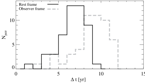
Figure 5.— Time baseline between the followup and SDSS observations. For 88% of the targets the rest frame $\Delta t>5$ yr.

3. Second-Epoch Optical Spectroscopy

We have conducted second-epoch optical spectroscopy for $50$ objects drawn from the offset sample presented in Section 2. We list all targets with second-epoch spectroscopy in Table 2. We preferentially selected brighter targets whenever available for better S/N. Our targets have median SDSS $r\sim 18.3$ mag. This “followup” sample is representative of the offset sample in general except that it is at lower redshifts (Figures 2–4). Figure 5 shows the distribution of rest-frame time intervals $\Delta t$ between the two epochs. In the following we describe details of the followup observations and data reduction.

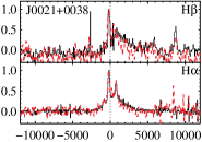
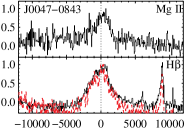
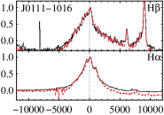
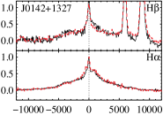
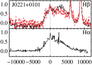
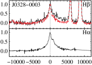
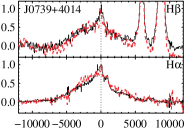
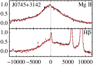
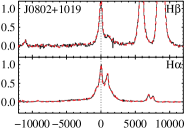
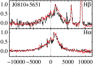
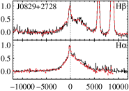
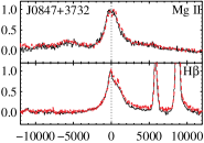
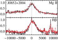
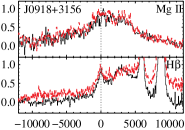
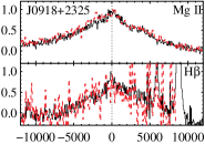
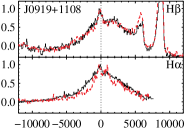
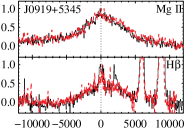
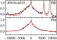
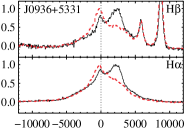
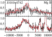
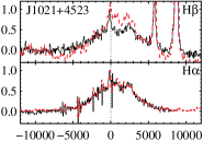
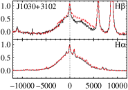
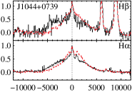
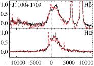
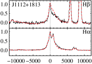
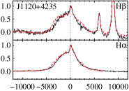
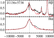
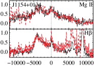
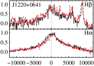
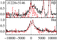
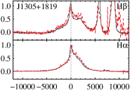
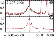
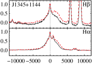
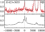
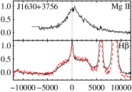
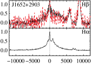
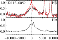
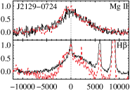
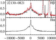
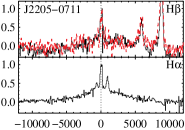
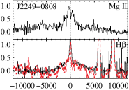
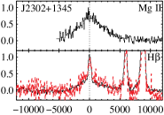
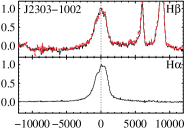
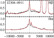
Relative Velocity (km s^-1)

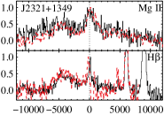
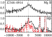
Figure 6.— Multi-epoch spectra (normalized for display purposes) of SDSS quasars with offset broad Balmer emission lines. The SDSS spectra are in solid black and followup spectra are in dashed red. For each object, the top (bottom) panel shows the H$\beta$ (H$\alpha$) or Mg II (H$\beta$) region, centered on the systemic redshift.

3.1. ARC 3.5 m/DIS

We observed nine targets using the Dual Imaging Spectrograph (DIS) on the Apache Point Observatory 3.5 m telescope on the nights of 2010 April 12, 16 and 2011 June 1 UT. The sky was non-photometric with varied seeing conditions ($1\farcs 1$–$1\farcs 6$ for April 12, $1\farcs 2$–$3\farcs 3$ for April 16, and $1\farcs 5$–$4\farcs 0$ for June 1). We adopted a $1\farcs 5\times$6^′ slit and the B1200+R1200 gratings centered at 4400 (or 5300) and 7200 (or 6700) Å. This wavelength set up covers the H$\beta$–[O III] $\lambda$5007 and H$\alpha$ (or Mg II) regions for targets at various redshifts. The slit was oriented at the parallactic angle at the time of observation. The spectral resolution is 1.8 (1.3) Å in FWHM (corresponding to $\sigma_{{\rm inst}}\sim$30–50 km s^-1) with a pixel scale of 0.62 (0.56) Å pixel^-1 in the blue (red) channel. Total exposure time varied between 2700 s and 4500 s (Table 2).

3.2. MMT/BCS

We observed 17 targets with the Blue Channel Spectrograph (BCS) on the 6.5 m MMT Telescope on the nights of 2011 July 30, 31, and December 26 and 27 UT. The sky was non-photometric with varied seeing conditions ($\lesssim 1$″ for July 30 and 31, 3″–5″ for December 26, and $\sim 1$″ for December 27). We adopted a $0\farcs 75\times$180″ slit and the 500 lines mm^-1 grating centered at 6000 Å with the UV36 filter. The slit was oriented at the parallactic angle at the time of observation. The spectral coverage was 3134 Å with a spectral resolution of $R=2800$ ($\sigma_{{\rm inst}}\sim$50 km s^-1) and a pixel scale of 1.2 Å pixel^-1. Total exposure time varied between 1200 s and 3600 s (Table 2).

3.3. FLWO 1.5 m/FAST

We observed 24 targets using the FAST spectrograph (Fabricant et al., 1998) on the 1.5 m Tillinghast Telescope at the Fred Lawrence Whipple Observatory (FLWO). Observations were carried out in queue mode over 19 nights from 2011 September to 2012 April. We employed the 300 lines mm^-1 grating with a $2^{\prime\prime}\times 180^{\prime\prime}$ slit oriented at the parallactic angle at the time of observation. The spectral coverage was $\sim 4000$ Å with a spectral resolution of $\sim 4$ Å ($\sigma_{{\rm inst}}\sim$90 km s^-1) and a pixel scale of 1.5 Å pixel^-1. The spectrograph was centered at different wavelengths depending on target redshift to cover their H$\beta$ and H$\alpha$ (or Mg II) regions. Table 2 lists the total exposure time for each object.

3.4. Data Reduction

We reduced the second-epoch optical spectra following standard IRAF procedures (Tody, 1986), with special attention to accurate wavelength calibration. Wavelength solutions were obtained using multiple HeNeAr lamp lines with rms of a few percent in a single exposure. Bright sky lines in the spectrum were used to correct for small errors in the absolute wavelength scale, which was corrected to heliocentric velocity. Flux calibration and telluric correction were applied after extracting one-dimensional spectra for each individual frame. We then combined all the frames to get a co-added spectrum for each target. Table 2 lists the S/N achieved in the final followup spectrum for each object. Figure 6 shows the second-epoch spectra compared against the original SDSS observations.

To measure the temporal velocity shift of the broad lines using cross-correlation analysis (ccf; Section 4.1; see also Paper I), we have re-sampled the second-epoch spectra so that they share the exact same wavelength grids (in vacuum) as the original SDSS spectra, which are linear on a logarithmical scale (i.e., linear in velocity space) with a pixel scale of $10^{-4}$ in log-wavelength, corresponding to 69 km s^-1.

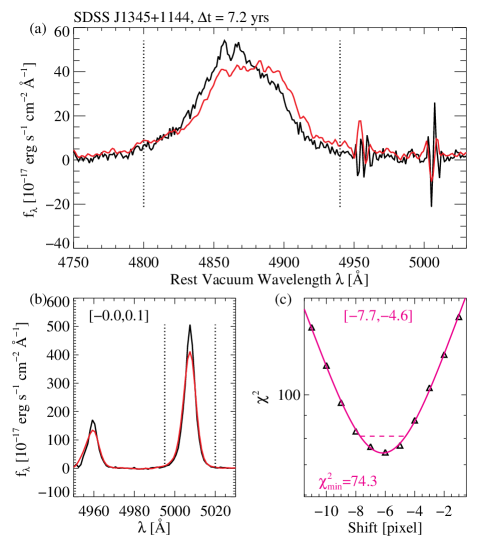
Figure 7.— Example of the cross-correlation analysis to measure the velocity shift of the broad H$\beta$ between two epochs. (a) Broad H$\beta$ spectrum of the original SDSS (black) and followup (red) observations. The spectral range of the cross-correlation analysis is marked by the dotted vertical lines. The followup spectrum has been scaled to match the integrated broad H$\beta$ line flux in the cross-correlation range. (b) Same as in panel (a), but for the narrow [O III] emission lines. Shown in brackets are the 99% confidence ranges (2.5$\sigma$) in units of pixels of the velocity shift of [O III] $\lambda$5007 (with 1 pixel corresponding to 69 km s^-1). Here and in other figures throughout the paper showing the cross-correlation analysis results, negative values mean that the emission line in the followup spectrum needs to be blueshifted to match that in the original SDSS spectrum (i.e., the emission line in the followup spectrum is redshifted relative to that in the original spectrum). (c) $\chi^{2}$ for the cross-correlation analysis of the broad H$\beta$ as a function of pixels. The solid magenta curve is the sixth-order B-spline fit of the 21 grid points centered on the one with the minimal $\chi^{2}$. The dashed horizontal segment indicates the $\Delta\chi^{2}=6.63(2.5\sigma)$ range, also indicated in the magenta brackets in units of pixels.

4. Measuring Radial Velocity Shift

We first describe our approach to quantify the velocity shifts in emission lines between two epochs (Section 4.1). We then discuss measurement uncertainties and caveats (Section 4.2).

4.1. Cross-correlation Analysis

We adopt a cross-correlation analysis (“ccf” for short) following the method discussed in Paper I (see also Eracleous et al., 2012). Cross-correlation analysis is preferred over approaches based on line fitting, which are more model dependent and are less sensitive to velocity shift. As shown with simulations in Paper I, ccf can in general achieve a factor of a few better sensitivity in velocity shift than direct line fitting.

The ccf finds the best-fit velocity shift $V_{\rm ccf}$ between the two epochs based on $\chi^{2}$ minimization (see Paper I for details). We have subtracted the pseudo-continua and narrow emission lines before analyzing the broad-line velocity shifts. We have fixed the narrow H$\beta$ to [O III] ratio to be consistent between two epochs. This helps minimize the error caused by incorrect narrow H$\beta$ subtraction due to model degeneracy. We use [O III] narrow emission lines, which are expected to show zero offset, to calibrate the absolute wavelength accuracy; we have subtracted off any nonzero velocity shifts detected in the [O III] lines from the broad-line velocity shift measurements (assuming that the nonzero shift in [O III] is due to wavelength calibration errors). In constraining the velocity shift of narrow [O III], we have subtracted the pseudo-continua and broad emission lines. Figures 7 and 8 show two examples of the ccf where a velocity shift is detected at the $>2.5\sigma$ significance level in broad H$\beta$; examples of no significant velocity shifts can be found in Paper I. Figure 7 shows a detection in broad H$\beta$ whose line profiles are consistent within uncertainties between two epochs, as quantified by various measures of line width and shape (FWHM and skewness). To double check that the velocity shift is real and not caused by some subtle changes in line profiles, we have also repeated the ccf with the broad-line-only spectrum smoothed with a Gaussian kernel with standard deviation $\sigma_{{\rm s}}$, and verified that the velocity shift does not change with varying $\sigma_{{\rm s}}$. Figure 8 shows a detection in broad H$\beta$ with significant line profile changes between two epochs as quantified by line widths. As further explained below in Section 5.4, we classify the former case as a BBH candidate and the latter as due to BLR variability around a single BH.

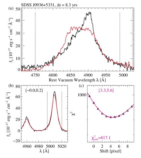
Figure 8.— Same as Figure 7, but for an example where the broad H$\beta$ profile changes significantly between two epochs.

4.2. Uncertainties

We now discuss the error budget of the line shift measurements. Residual errors from wavelength calibration should be minor, because (1) we have calibrated absolute redshift using simultaneous constraints on the narrow emission lines based on [O III] ccf; and (2) the relative wavelength accuracy has been calibrated to within a few percent using multiple lamp exposures and has been further verified by independent measurements using a second broad line (H$\alpha$ or Mg II). Errors due to absolute flux calibration should not be a major issue either, because we have subtracted the pseudo-continua. The spectra have been normalized to have the same integrated broad-line flux. Relative spectrophotometric flux calibration in principle can introduce substantial uncertainty in the velocity shift measurement, but for most targets we can constrain such effects by considering independent measurements from a second broad line.

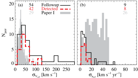
Figure 9.— Distribution of the measurement uncertainties of (a) broad-line velocity shift and (b) broad-line rest-frame acceleration. Numbers indicate median values of measurement uncertainty for different samples.

Figure 9 shows distributions of the measurement uncertainty of broad-line velocity shift $\sigma_{V_{{\rm ccf}}}$ and acceleration $\sigma_{a_{{\rm ccf}}}$. They were estimated from the 99% confidence ranges of the $\chi^{2}$ curves as listed in Table 2. Recall that the measurement errors in the velocity shift of broad emission lines increase with increasing line width and decreasing S/N (Paper I). Compared to the “superior” sample of Paper I, the median $\sigma_{V_{{\rm ccf}}}$ of the followup sample is $\sim 85$% larger. This is expected for two reasons: (1) the broad H$\beta$ FWHM of the followup sample is on average $\sim 25$% larger than that of ordinary quasars (Figure 4); and (2) the SDSS spectrum S/N of the followup sample is comparable to that of the superior sample but our new second-epoch spectra have lower S/N in general. However, the typical $\sigma_{a_{{\rm ccf}}}$ of the followup sample is $\sim 65$% smaller than that of the superior sample of Paper I, due to longer time baselines.

5. Results

We present the detection frequency of broad-line shifts for offset quasars in Section 5.1. We then examine the acceleration distribution and compare to the general quasar population studied in Paper I (Section 5.2). In Section 5.3 we study the relation between velocity offset in single-epoch spectra and acceleration between two epochs. Finally we discuss the likely scenario for each individual detection in Section 5.4.

5.1. Detection Frequency

In Table 2 we list the velocity shifts measured from ccf along with their statistical uncertainties (99% confidence). Out of the 50 followup targets, 24 show significant broad-line velocity shifts between the two epochs. We show the two-epoch broad H$\beta$ lines for all of these 24 quasars in Figures 10–12. Also shown are the [O III] lines (for determining the systemic velocity) and broad H$\alpha$ (or Mg II) if available (to check for consistency).

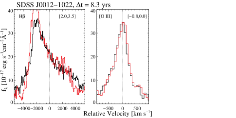
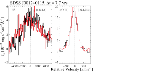
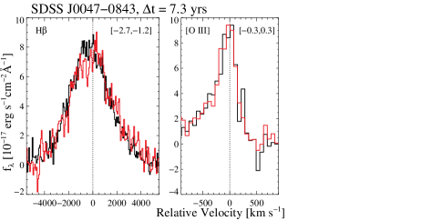
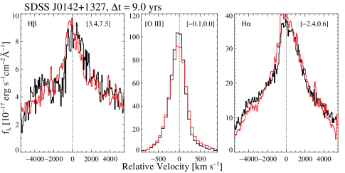
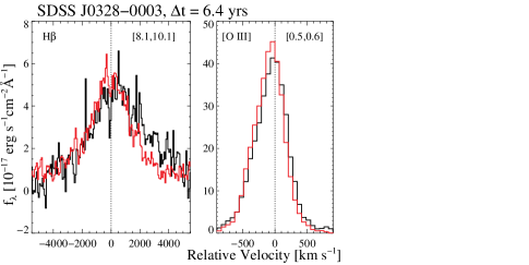
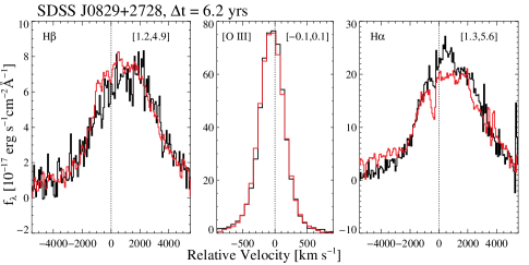
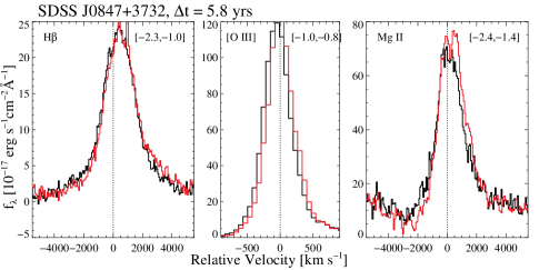
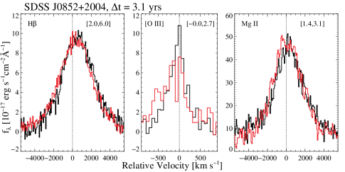
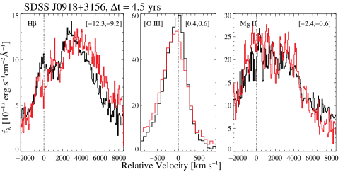
Figure 10.— Emission line spectra at two epochs for the 24 quasars with detections of significant acceleration (together with those shown in Figures 11 and 12). Black is for the original SDSS observations and red is for followups. The followup spectra are scaled to match the emission line fluxes of the SDSS observations. For each object, we show the broad H$\beta$ and [O III] $\lambda$5007 lines in velocity space centered at the systemic velocity (noted by dotted lines). Also shown are the broad H$\alpha$ (or Mg II) results when available. In each panel we list the velocity shift between the two epochs in brackets enclosing the 2.5$\sigma$ confidence range in units of pixels (with 1 pixel being 69 km s^-1). Here, negative values mean that the emission line in the followup spectrum needs to be blueshifted to match that in the original SDSS spectrum (i.e., the emission line in the followup spectrum is redshifted relative to that in the original spectrum). See Section 5.4 for details.

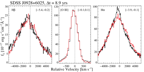
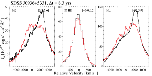
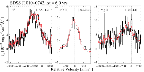
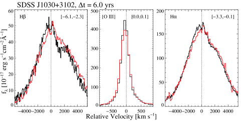
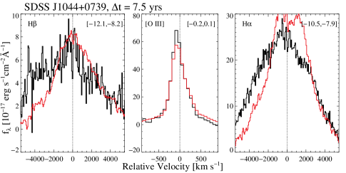
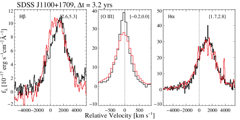
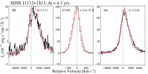
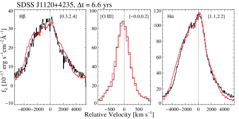
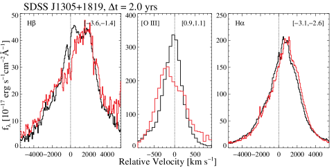
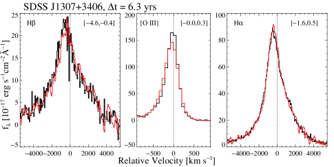
Figure 11.— Same as Figure 10, but for another set of detections.

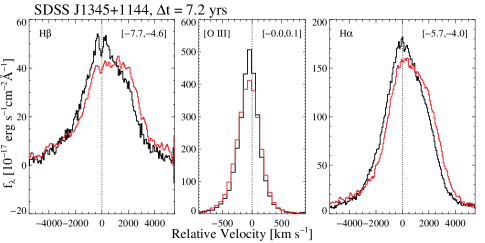
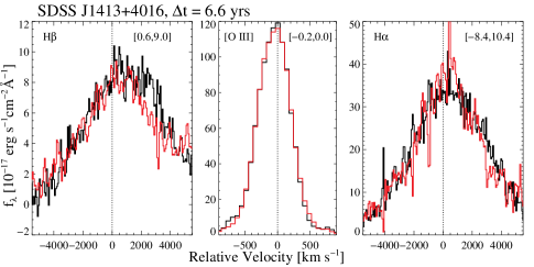
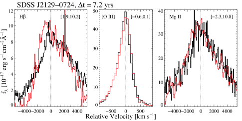
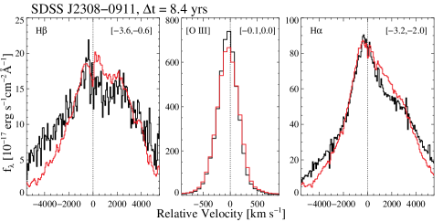
Figure 12.— Same as Figure 10, but for another set of detections.

We now compare the detection fraction with that of the general quasar population studied in Paper I. We account for differences in time separation and measurement sensitivity. The detection fraction in normal quasars (among the “good” sample) increases with time separation (Paper I); it is $\lesssim$ a few percent at $\Delta t<1$ yr, and increases to $\sim$20% at $\Delta t>3$ yr. Naively extrapolating the time dependence (Figure 11 of Paper I) would imply a detection fraction of $\sim$30% $\pm$ 10% at $\Delta t>5$ yr. This prediction is marginally lower than the detection fraction we find in this paper ($\sim$50% $\pm$ 10%) at $\Delta t>5$ yr. The difference becomes more prominent considering that the velocity shift uncertainty of the followup sample is $\sim 25$% larger than that of the good sample in Paper I (median $\sigma_{V_{{\rm ccf}}}\sim 50$ compared to $\sim$40 km s^-1). Among the detections, the fraction of BBH candidates (9 out of 24 or $40$% $\pm$ 10%; see Section 5.4.1 for details) is consistent with that of Paper I (7 out of 30 or 25% $\pm$ 10%) within uncertainties, although Paper I had less stringent constraints on objects that show significant line profile changes, because contamination by double-peaked broad lines is less common in the general quasar population.

In summary, these results suggest that the frequency of broad-line shifts in offset quasars might be higher than that in the general quasar population on timescales of more than a few years. Of course, this is expected in the BBH scenario since both velocity offsets and shifts in these offsets are due to the orbital motion of the BBH. However, the statistics are poor and the results are still consistent with having no difference between the two populations.

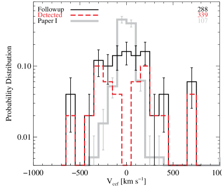
Figure 13.— Distribution of the broad-line velocity shift between two epochs. Error bars indicate Poisson uncertainties. Numbers in the upper-right corner indicate standard deviations for different samples.

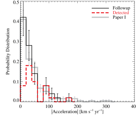
Figure 14.— Probability distribution of the rest-frame broad-line acceleration between two epochs. Error bars indicate Poisson uncertainties. The observed distribution of the followup sample is consistent with that found in Paper I within uncertainties. Since the followup sample in this paper has smaller measurement errors in acceleration than the “superior” sample in Paper I (Figure 9), this suggests a broader (by $\sim 30$%) intrinsic acceleration distribution in the followup sample of offset quasars than in normal quasars (See Section 5.2 for details).

5.2. Acceleration Distribution

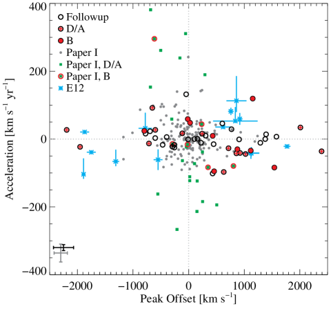
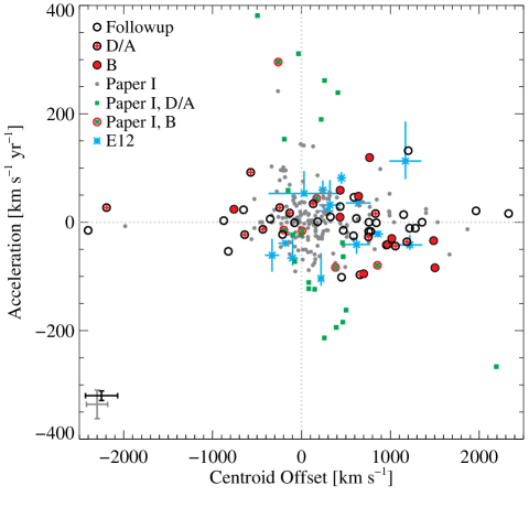
Figure 15.— Left: broad H$\beta$ rest-frame acceleration vs. peak velocity offset (estimated from the original SDSS spectrum). Positive offsets mean redshifted broad emission lines from the systemic velocities; positive accelerations indicate more redshifted broad lines in the followup spectra than those in the original SDSS spectra. We show objects without significant broad-line velocity shifts in the followup sample as black open circles (26 objects). We also show the 24 cases with significant broad-line velocity shifts, including 9 binary candidates (labeled with “B” and shown as red filled circles), and 15 BLR variability or ambiguous cases (labeled with “D/A” (which is short for “disk emitters or ambiguous”) and shown as black open circles with red plus signs). Shown for comparison are the superior sample (gray dots) and the velocity-shift detected sample (green filled squares with red open circles for binary candidates, and green filled squares for BLR variability or ambiguous cases) of Paper I. The black error bars in the lower left corner indicate typical uncertainties of the followup sample, whereas the gray error bars denote those of the superior sample in Paper I. Also shown for comparison is the velocity-shift detected sample of Eracleous et al. (2012, cyan asterisks with error bars). Right: same as left panel, but for centroid velocity offset. There is a weak correlation (Spearman $P_{{\rm null}}\sim 10^{-3}$) in both the shift-detected samples of this work and of Paper I, except perhaps the few objects with the most extreme offset velocities (i.e., $>10^{3}$ km s^-1). See Section 5.3 for details.

Figure 13 shows the observed distribution of broad-line shifts of the followup sample compared with that of the superior sample of Paper I. The velocity shift distribution of offset quasars is 1.7 times wider than that of normal quasars. The statement still holds for the intrinsic velocity shift distribution after accounting for the difference in measurement errors (Figure 9). From $V_{{\rm ccf}}$ and $\Delta t$, we then estimate $a_{{\rm ccf}}$, the average acceleration between two epochs, as listed in Table 2. Figure 14 shows the distribution of the absolute value of the measured acceleration of the followup sample compared with the superior sample of Paper I.

The measured acceleration distribution of the followup sample is consistent with the superior sample of Paper I. After accounting for the difference in measurement errors (Figure 9), the inferred intrinsic acceleration distribution of the followup sample is $\sim 30$% wider than that of the superior sample of Paper I. However, the timescales being probed are very different ($>$5 yr in this work compared to an average of $\sim 1$ yr in Paper I) so a fair comparison is difficult.

5.3. Velocity Offset Versus Acceleration

We now examine the relation between broad-line velocity offset (relative to systemic) and acceleration. Figure 15 shows the broad H$\beta$ peak velocity offset of the original SDSS spectrum versus the radial acceleration between the two epochs. We show our followup sample, the superior sample of Paper I, and the sample with detected velocity shifts from Eracleous et al. (2012). We find a tentative anti-correlation (Spearman $P_{{\rm null}}=10^{-3\pm 0.5}$ and $\rho=-0.13\pm 0.01$, where the 1$\sigma$ errors were estimated from bootstrap tests) between peak $V_{{\rm off}}$ and $a_{{\rm ccf}}$ in our combined sample (i.e., the “superior” sample of Paper I (193 pairs of observations) plus our followup sample (50 pairs of observations)). The velocity offset and accelerations tend to have opposite signs, in the sense that blueshifted (redshifted) broad emission lines in the single-epoch spectra on average tend to become less blueshifted (redshifted) in the followup spectra after a few years. A tentative anti-correlation is also detected in the subset of detected objects (i.e., the 54 objects with significant velocity shifts from Paper I and our followup sample) but is weaker ($P_{{\rm null}}\sim 10^{-2}$ and $\rho\sim-0.3$), probably due to poorer statistics.

Figure 15 also shows the same results based on the centroid offset. Again, there is a tentative anti-correlation ($P_{{\rm null}}=10^{-3\pm 0.2}$) between centroid $V_{{\rm off}}$ and $a_{{\rm ccf}}$ both in the combined sample ($\rho=-0.14\pm 0.01$) and in its subset with detected shifts ($\rho=-0.36\pm 0.02$). These weak anti-correlations are only suggestive and would need to be confirmed with larger samples. We expect no correlation between the velocity and the instantaneous acceleration in the BBH scenario, but see Section 6.2 for further discussion on the implications of these results in the context of identifying candidate BBHs.

5.4. Individual Detections

As listed in Table 2, we divide the 24 detections into three categories following Paper I according to different possible origins of the observed broad-line velocity shifts: (1) BBH candidates, (2) broad-line variability, and (3) ambiguous cases. These categories are only meant to be our best attempt at an empirical classification and are by no means rigorous. Below we present these classifications and comment on individual cases.

5.4.1 BBH Candidates

We categorize nine objects as BBH candidates (Table 2). The criteria are (1) broad-line velocity shifts are detected between two epochs ($>99$% confidence); (2) there is an overall bulk velocity shift (i.e., the measured velocity shift is not solely caused by a profile change); and (3) the velocity shifts independently measured from broad H$\beta$ and broad H$\alpha$ (or Mg II) are consistent within uncertainties. While the presence of broad-line profile changes without bulk velocity shifts does not necessarily rule out the possibility of BBHs (e.g., Shen & Loeb, 2010), we assign these cases as BLR variability (e.g., due to disk emitters) to minimize contamination (Section 5.4.2). This criterion rejects more candidates when applied to the present sample compared to the sample in Paper I (20% compared to 10%), because dramatic profile changes are much more commonly seen in offset quasars than in normal quasars. Below we comment on each case. In Section 6.3 we discuss implications of our results for the model parameters under the BBH hypothesis.

J082930.60+272822.7. We detect consistent velocity shifts over 6.2 yr in broad H$\beta$ and broad H$\alpha$ with no significant line profile changes. The radial acceleration measured from broad H$\beta$ is [$-54$, $-13$] km s^-1 yr^-1 (2.5$\sigma$). This object was also noted by Eracleous et al. (2012) and by Tsalmantza et al. (2011), but no second-epoch spectrum was available.

J084716.04+373218.1. Consistent velocity shifts over 5.8 yr are detected in broad H$\beta$ and Mg II with no significant line profile change. The radial acceleration measured from broad H$\beta$ is [3, 18] km s^-1 yr^-1 (2.5$\sigma$).

J085237.02+200411.0. Broad H$\beta$ and Mg II show consistent velocity shifts over 3.1 yr with no significant line profile change. The radial acceleration measured from broad H$\beta$ is [$-133$, $-43$] km s^-1 yr^-1 (2.5$\sigma$).

J092837.98+602521.0. Broad H$\beta$ and H$\alpha$ show consistent velocity shifts over 8.9 yr with no significant line profile change. The radial acceleration measured from broad H$\beta$ is [1, 42] km s^-1 yr^-1 (2.5$\sigma$).

J103059.09+310255.8. Broad H$\beta$ and H$\alpha$ show consistent velocity shifts over 6.0 yr with no significant line profile change. The radial acceleration measured from broad H$\beta$ is [26, 70] km s^-1 yr^-1 (2.5$\sigma$).

J110051.02+170934.3. Broad H$\beta$ and H$\alpha$ show consistent velocity shifts over 3.2 yr with no significant line profile change. The radial acceleration measured from broad H$\beta$ is [$-113$, $-55$] km s^-1 yr^-1 (2.5$\sigma$). This object was also noted by Eracleous et al. (2012), but no second-epoch spectrum was available.

J111230.90+181311.4. Consistent velocity shifts over 4.1 yr are detected in broad H$\beta$ and H$\alpha$ with no significant line profile change. The radial acceleration measured from broad H$\beta$ is [$-51$, $-8$] km s^-1 yr^-1 (2.5$\sigma$).

J130534.49+181932.9. Consistent velocity shifts over 2.0 yr are detected in broad H$\beta$ and H$\alpha$ with no significant line profile change. The radial acceleration measured from broad H$\beta$ is [80, 158] km s^-1 yr^-1 (2.5$\sigma$). This object was also noted by Eracleous et al. (2012). The authors found no significant shift in the H$\beta$ region based on a spectrum taken 1.9 yr after the original SDSS observation; no second-epoch spectrum was available for the H$\alpha$ region.

J134548.50+114443.5. This object has the largest velocity shift detected among the BBH candidates in our sample. Consistent velocity shifts over 7.2 yr are detected in broad H$\beta$ and H$\alpha$ with no significant line profile change. The radial acceleration measured from broad H$\beta$ is [44, 73] km s^-1 yr^-1 (2.5$\sigma$).

5.4.2 Alternative Scenarios

As listed in Table 2, there are five objects for which we suggest that broad-line variability likely causes the observed velocity shifts. Although we tried to eliminate double-peaked broad emission lines in the original sample selection based on single-epoch spectra, the rejection was incomplete. These objects usually have more complicated broad-line profiles than the BBH candidates. The line profile changes between two epochs are more dramatic, similar to some of the well-monitored double-peaked broad lines which are generally explained as disk emitters known in the literature. This is in contrast to the findings in Paper I that significant profile changes are uncommon in the general quasar population (over timescales less than a few years). The cases with dramatic line profile changes in our followup sample exhibit similar velocity shifts in broad H$\beta$ and broad H$\alpha$ (or Mg II). However, the velocity shifts measured from ccf are mostly caused by profile changes instead of bulk velocity shifts. Below we comment on each case.

J001224.02$-$102226.5. We detect a velocity shift over 8.3 yr in broad H$\beta$. The broad H$\beta$ line, and in particular the broad base of the line profile, got narrower, similar to the profile change reported in broad H$\alpha$ by Decarli et al. (2013). The radial acceleration measured from broad H$\beta$ is [$-29$, $-16$] km s^-1 yr^-1 (2.5$\sigma$), consistent with the acceleration ($-32^{+17}_{-26}$ km s^-1 yr^-1) reported in broad H$\alpha$ by Decarli et al. (2013) based on a spectrum taken 8.1 yr after the original SDSS observation. This object was also noted by Shen & Loeb (2010), Zamfir et al. (2010), and Eracleous et al. (2012). Eracleous et al. (2012) reported a velocity shift of $+125^{+35}_{-30}$ km s^-1 in the H$\beta$ region based on a spectrum taken 6.8 yr after the original SDSS observation; no second-epoch spectrum was available for the H$\alpha$ region.

J093653.84$+$533126.8. This object has among the most dramatic profile changes in our followup sample. The redshifted peaks of broad H$\beta$ and H$\alpha$ appear to have blueshifted by $>2000$ km s^-1 over 8.3 yr, while no obvious shifts were seen in the bases of the broad lines. Eracleous et al. (2012) reported a profile change in the H$\beta$ region similar to our findings based on a spectrum taken 6.7 yr after the original SDSS observation; no second-epoch spectrum was available for the H$\alpha$ region. Decarli et al. (2013) also reported a similar profile change in the H$\beta$ and H$\alpha$ regions based on a spectrum taken 7.5 yr after the original SDSS observation.

J104448.81$+$073928.6. This object is also among those with the most dramatic profile changes. The line widths of broad H$\beta$ and broad H$\alpha$ appear to have narrowed by $\sim$30%–40% over 7.5 yr.

J112007.43$+$423551.4. Broad H$\beta$ and H$\alpha$ show consistent velocity shifts over 6.6 yr, but the shifts are mostly due to changes in the line profile rather than bulk velocity shifts. The blueshifted shoulder of broad H$\beta$ also becomes more prominent in the second-epoch spectrum, which is reminiscent of double-peaked broad emission lines generally interpreted as disk emitters.

J230845.60$-$091124.0. Broad H$\beta$ and H$\alpha$ show consistent velocity shifts over 8.4 yr, but the shifts are mostly due to changes in line profiles rather than bulk velocity shifts.

We classify the rest of the objects with broad H$\beta$ velocity shifts as “ambiguous” (Table 2). These objects either do not have followup spectra for a second broad line, or that they do but the measured velocity shifts are inconsistent with those from broad H$\beta$. More observations with wider spectral coverage and enhanced S/N are needed to better determine the nature of these objects.

6. Discussion

6.1. Comparison with Previous Work

Recently Eracleous et al. (2012) carried out the first systematic spectroscopic followup study of quasars with offset broad H$\beta$ lines. The authors identified 88 quasars from the SDSS DR7 with offsets of $\gtrsim 1000$ km s^-1. Compared to our offset sample, the Eracleous et al. (2012) sample has larger broad-line velocity offsets, focusing on the most extreme objects. Among the 68 objects for which Eracleous et al. (2012) conducted second-epoch spectroscopy, 14 were found to show significant velocity shifts after rejecting objects with significant line profile changes. This fraction ($\sim 20$% or 14 out of 68) is similar to that of our “BBH candidates” category (9 out of 50). Eracleous et al. (2012) found no relation between the acceleration and the initial velocity offset, although their sample size may be too small to see any weak (anti-)correlation. Another possibility for the null correlation is that the Eracleous et al. (2012) sample focuses on more extreme velocity offsets (i.e., $>10^{3}$ km s^-1) than our samples, where the anti-correlation between $V_{{\rm off}}$ and $a_{{\rm ccf}}$ seems to break down.

The existing data cannot prove that the “BBH candidates” reported in this work are indeed BBHs. To further test the BBH hypothesis would require future observations, most importantly more followup observations to confirm or reject whether the RV curve follows the expected binary motion. The time baselines required to detect a significant fraction of an orbit may be too long to be practical considering that the expected orbital periods range from a few decades to a few centuries (Table 3), but linear growth of the velocity shift with time without significant variation in the profile shape would already be a strong signature. Despite the tentative nature of the evidence so far, in the following sections we focus the discussion on implications of our results under the BBH hypothesis, as it is the main motivation of the current work.

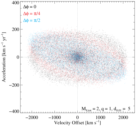
Figure 16.— Illustration of the effect of orbital phase in modulating the correlation between the observed first-epoch velocity offset and the average acceleration between two epochs (Figure 15). The acceleration is calculated as $(V(I,\phi+\Delta\phi)-V(I,\phi))/\Delta t$, where $\Delta t=P\Delta\phi/2\pi$ is the time separation between two epochs with $P$ being the orbital period. Black, red, and cyan color denote the cases when $\Delta t$ is $0$, $1/4$, and $1/8$ of $P$, respectively. Shown for each $\Delta\phi$ are measurements of $10^{4}$ mock orbits assuming random orbital inclination and phase for an equal-mass BBH with $2\times 10^{8}~{}M_{\odot}$ total BH mass, and a circular orbit with a binary separation of 0.05 pc (orbital period $P=75$ yr). Gaussian noises with standard deviations $80$ km s^-1 and $20$ km s^-1 yr^-1 have been added to the velocity offsets and accelerations, respectively. A correlation similar to the observed ones (Figure 15) arises when $\Delta t$ is a non-negligible fraction of $P$ (further shown in Figure 17). See Section 6.2 for more discussion, and the Appendix for more details on model assumptions and parameter definitions.

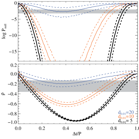
Figure 17.— Spearman correlation coefficients $\rho$ and $P_{{\rm null}}$ of $a$ and $V$ as a function of $\Delta t/P$. At a given $\Delta t/P$, $\rho$ and $P_{{\rm null}}$ are calculated using 243 data points (matching the size of our combined sample) drawn from $10^{3}$ realizations of $10^{4}$ mock orbits generated assuming zero eccentricity and random orbital inclination and phase. Gaussian noises with standard deviations $80$ km s^-1 and $20$ km s^-1 yr^-1 have been added to the velocity offsets and accelerations, respectively. Solid curves denote the median values whereas the dashed curves indicate 1$\sigma$ confidence intervals. Gray shaded areas represent ranges of the observed correlation coefficients (measured from the combined sample using peak or centroid velocities). As in Figure 16, the baseline model (shown in black) assumes an equal-mass BBH with $2\times 10^{8}~{}M_{\odot}$ total BH mass, and a binary separation of 0.05 pc (orbital period $P=75$ yr). Shown in color are models with larger separations. See Section 6.2 for more discussion.

6.2. Implications for Identifying BBH Candidates

There is a tentative anti-correlation between broad-line velocity offset and acceleration (Section 5.3). In the BBH scenario, both RV and acceleration are determined by the binary separation, masses of the two BHs, orbital phase $\phi$, and orbital inclination $I$ to the line of sight (LOS). The similar distributions in virial BH mass, quasar luminosity and broad H$\beta$ FWHM (Figures 2 and 4) suggest that the intrinsic properties of offset-line quasars are similar to those of normal quasars. It is therefore unlikely that the selection of larger offset velocities has induced any major bias in terms of BH mass and accretion rate. On the other hand, selecting for larger velocity offsets in single-epoch spectra could preferentially yield BBHs with smaller binary separations and/or larger values of $|\sin I|$ and $|\sin\phi|$.

Any model in which the broad-line offsets are due to BBHs makes several clean predictions (assuming random orbital phases and a selection function that depends only on the absolute value of the velocity offset): (1) the distribution of velocity offsets should be symmetric around zero (after correcting for gravitational redshift); (2) the distribution of accelerations should be symmetric around zero; (3) there should be no correlation between velocity $V(I,\phi)$ and the instantaneous acceleration $a(I,\phi)$, i.e., for fixed $V$ the probability of seeing $a$ and $-a$ should be the same (since $\pi-\phi$ is just as likely as $\phi$); and (4) there should be a weak anti-correlation between $|V(I,\phi)|$ and $|a(I,\phi)|$ since they are out of phase by $90^{\circ}$ at least for circular orbits.

For our offset sample, (1) is violated, but as we discussed (Section 2.1.5), this is likely a selection bias; (2) is satisfied; both (3) and (4) are violated. A possible explanation is that we measure the average acceleration over the interval $\Delta t$, rather than the instantaneous acceleration, and these are not the same if $\Delta t$ is a significant fraction of the orbital period $P$. Figure 16 illustrates such an effect. We show the measurements of $10^{4}$ mock orbits assuming zero eccentricity and random orbital inclination and phase for an equal-mass BBH with $2\times 10^{8}~{}M_{\odot}$ total BH mass, and a binary separation of 0.05 pc (orbital period $P=75$ yr). Gaussian noises with standard deviations 80 km s^-1 and 20 km s^-1 yr^-1 (typical for the measurements in our combined sample) are added to the velocity offsets and accelerations, respectively. Different colors denote the cases when $\Delta t$ is 0, 1/4, and 1/8 of $P$. An anti-correlation arises when $\Delta t$ is a non-negligible fraction of $P$, similar to that observed in Figure 15.

Figure 17 shows more quantitative results. It plots the Spearman correlation coefficients $P_{{\rm null}}$ and $\rho$ of the acceleration $a$ and velocity $V$ as a function of $\Delta t/P$. At a given $\Delta t/P$, the coefficients are calculated using 243 data points (matching the size of our combined sample) drawn from $10^{3}$ realizations of $10^{4}$ mock orbits assuming zero eccentricity and random orbital inclination and phase. As in Figure 16, the baseline model assumes an equal-mass BBH with $2\times 10^{8}~{}M_{\odot}$ total BH mass, and a binary separation of 0.05 pc (orbital period $P=75$ yr). Again, Gaussian noises with standard deviations 80 km s^-1 and 20 km s^-1 yr^-1 are added to the velocity offsets and accelerations, respectively. Also shown are models with the same masses but at larger binary separations, which result in larger correlation coefficients (i.e., weaker anti-correlations) because of the smaller S/N due to the smaller velocity and acceleration amplitudes. The coefficients observed in our samples are shown as gray shaded areas. The comparison between the data and the baseline model suggests $\Delta t/P\gtrsim 0.05$–0.1 since there must be some dilution of the correlation due to objects in the data that are not BBHs. Thus the observed velocity–acceleration anti-correlation may suggest that the typical orbital period is $\sim 10$–20 times the typical time baseline (which is $\sim 1$ yr for the superior sample in Paper I, or $\sim 3$–10 yr for the followup sample in this work), or $\sim 30$–200 yr for our followup sample, which is consistent with our estimates for individual candidates (see Section 6.3). These numbers are only crude estimates. Nevertheless, the result does suggest that the time baselines of our observations are a significant fraction of the orbital period, regardless of whether the velocity shifts are due to BBHs or some other periodic feature such as an orbiting clump or cloud in the BLR.

An alternative explanation why quasars with offset broad emission lines are more likely to exhibit accelerations might be BLR variability is likely to produce both velocity offsets and accelerations, and the statistical properties of the stochastic process producing the velocity offsets and accelerations leads to an observed anti-correlation between velocity offset and acceleration measured over a nonzero time interval.

Table 3Estimated Model Parameters for the Binary Black Hole Candidates

			$q=2$				$q=0.5$
	${\rm log}M_{1}$	$R_{{\rm BLR}}$	$f_{r}^{-1}R_{{\rm BLR}}$	$d$	$P$	$t_{{\rm gr}}$	$f_{r}^{-1}R_{{\rm BLR}}$	$d$	$P$	$t_{{\rm gr}}$
SDSS Designation	($M_{\odot}$)	(pc)	(pc)	(pc)	(yr)	(Gyr)	(pc)	(pc)	(yr)	(Gyr)
(1)	(2)	(3)	(4)	(5)	(6)	(7)	(8)	(9)	(10)	(11)
082930.60$+$272822.7	8.6	0.046	0.15	0.24	320	5	0.11	0.071	72	0.3
084716.04$+$373218.1	8.1	0.054	0.17	0.29	720	260	0.12	0.13	290	70
085237.02$+$200411.0	8.4	0.058	0.18	0.13	160	1	0.13	0.063	74	0.6
092837.98$+$602521.0	8.9	0.071	0.22	0.46	580	7	0.16	0.21	260	3
103059.09$+$310255.8	8.7	0.043	0.13	0.25	300	3	0.098	0.11	130	1
110051.02$+$170934.3	8.2	0.041	0.13	0.092	120	2	0.093	0.026	27	0.1
111230.90$+$181311.4	7.9	0.029	0.091	0.12	230	30	0.066	0.032	47	1
130534.49$+$181932.9	8.3	0.029	0.090	0.10	120	1	0.065	0.043	49	0.4
134548.50$+$114443.5	8.1	0.031	0.097	0.11	180	7	0.071	0.051	77	2

Note. — Column 2: virial BH mass estimate for the active BH taken from Shen et al. (2011b); Column 3: BLR size estimated from the 5100 Å continuum luminosity assuming the empirical $R$-$L_{5100}$ relation in Bentz et al. (2009); Columns 4–11: estimated BBH model parameters, assuming orbital inclination $I=45^{\circ}$ (slightly smaller than the median inclination for random orientations ($I=60^{\circ}$) because edge-on quasars are more likely to be obscured) and varying mass ratio $q=2$ or $0.5$, where $q\equiv M_{2}/M_{1}$. $f_{r}^{-1}R_{{\rm BLR}}$ (Columns 4 and 8) is the estimated lower limit for the binary separation $d$ (Columns 5 and 9), if we require that the BLR size is smaller than the Roche radius (see the Appendix for details). The condition $d>f^{-1}_{r}R_{{\rm BLR}}$ is met for $q=2$ in all cases considering uncertainties. Columns 6 and 10: binary orbital period $P$; Columns 7 and 11: orbital decay timescales due to gravitational radiation. See Sections 6.3 and 6.5 and the Appendix for more discussion.

6.3. Constraints on BBH Model Parameters

We now discuss the implications of our results for BBH model parameters. As demonstrated in Paper I for the general quasar population, the observed distribution of broad-line radial accelerations can be used to place constraints on a hypothetical BBH population. However, this exercise cannot be straightforwardly implemented for offset-line quasars, because (1) as discussed above, there is likely a selection bias in orbital phase. This needs to be properly accounted for in order to translate the observed acceleration distribution into unbiased constraints on BBH parameters. However, the specific selection function is unclear because of the complication due to visual selection; and (2) the size of the followup sample is too small to derive robust statistical constraints as we did in Paper I.

In view of these difficulties, we adopt here a different approach: we derive model parameters for the purported BBH candidates, using plausible assumptions for the orbital inclination $I$ and mass ratio $q\equiv M_{2}/M_{1}$. Following Paper I, we assume that the BBH is on a circular orbit and that only BH number 1 is active and powering the observed BLR. We then set the velocity $V_{1}$ equal to the average of the broad-line velocity offsets from the SDSS and followup spectra, and determine the acceleration $a_{1}$ from the difference in these offsets. We adopt the mass $M_{1}$ from the virial BH mass estimate and the radius of the BLR from the 5100 Å continuum luminosity, both taken from Shen et al. (2011b). Then we find the orbital phase $\phi$ and binary separation $d$ as described in the Appendix. We then make the following consistency checks. The binary separation $d$ should at least satisfy $d>R_{{\rm BLR}}$ for the model to be self-consistent. If we further require that the BLR size is smaller than the Roche radius, the binary separation must also satisfy $d>f^{-1}_{r}R_{{\rm BLR}}$, where $f_{r}$ is the average radius of the Roche lobe in a circular binary system (Equation (A3)).

Table 3 lists model parameters for the nine BBH candidates. The baseline model assumes $I=45^{\circ}$, slightly smaller than the median inclination for random inclinations ($I=60^{\circ}$) because edge-on quasars are more likely to be obscured, and $q=2$, because some theoretical work (e.g., Dotti et al., 2006) suggests that the less massive BH in a BBH is more likely to be active. For the baseline model, both conditions on the separation are met for all candidates; $d$ is $\sim$2–7 times larger than the BLR size $R_{{\rm BLR}}$. As discussed in Paper I, one caveat in these arguments is that our adopted BLR size is estimated from the $R$–$L$ relation (Bentz et al., 2009) found by reverberation mapping studies, which represents the emissivity-weighted average radius and could be an underestimate of the actual size. Nevertheless the bulk of the line emission should come from within the adopted BLR size. Models with smaller mass ratios (e.g., $q=0.5$) are less favored, because the Roche condition is violated in most cases (six out of nine), unless the inclination angle is higher than the random case (i.e., $I>60^{\circ}$). Models with much larger mass ratios (i.e., $q\gg 1$) are possible but perhaps also less likely, because the resulting total BH mass would be too large for the galaxies to obey the $M_{{\rm BH}}$–$\sigma_{\ast}$ relation observed in local inactive galaxies (e.g., Gültekin et al., 2009, assuming that quasar host galaxies follow the same relation as local inactive galaxies and that the gas velocity dispersion can be used as an approximate surrogate for the stellar velocity dispersion $\sigma_{\ast}$).

These tests suggest that there is some permitted parameter space in the BBH model that explains our observations for the nine suggested BBH candidates. While they neither validate the BBH hypothesis nor prove our oversimplified model assumptions, these tests do show that our models are self-consistent, and suggest that they provide a viable explanation of the data.

6.4. Implications for BBH Orbital Evolution

The model parameters that we derived in the previous section are based on the assumption that the binary separation is larger than the BLR size so that the broad-line bulk velocity would trace binary orbital motion. Under this assumption, our followup sample is most sensitive to $d\lesssim 1$ pc given the acceleration measurement accuracy (median 1$\sigma$ error of $\sim 10$ km s^-1 yr^-1) and the estimated BH masses. However, this assumption is not necessarily true, even if the observed broad-line velocity shift is indeed caused by BBH orbital motion. If the binary separation is smaller than typical BLR sizes (e.g., $d<0.05$ pc), the relation between orbital frequency and the temporal broad-line velocity shift would be more complicated (e.g., Bogdanović et al., 2008; Shen & Loeb, 2010).

Stellar dynamics simulations suggest that the orbital evolution of BBHs in spherical galaxies may stall at $\sim$pc scales (e.g., Begelman et al., 1980; Milosavljević & Merritt, 2001; Yu, 2002; Vasiliev et al., 2014, the so-called “final-parsec” problem), but the barrier may be overcome in more realistic models of triaxial or axisymmetric galaxies (e.g., Yu, 2002; Merritt & Poon, 2004; Preto et al., 2011; Khan et al., 2013, but see Vasiliev et al. 2014) or in gaseous environments (e.g., Gould & Rix 2000; Escala et al. 2005; but see Lodato et al. 2009; Chapon et al. 2013). If some of the suggested sub-pc BBH candidates (Section 5.4.1) were confirmed with future long-term spectroscopic monitoring, and their gravitational radiation decay timescales were less than the Hubble time (discussed below in Section 6.5), the presence of such systems would be evidence that the final-parsec barrier can be overcome at least in some quasar host galaxies.

6.5. Implications for GW Source Density

Assuming that the suggested candidates (Section 5.4.1) are indeed BBHs in which one member is active, our results would indicate a lower limit for the fraction of sub-pc BBHs in SDSS quasars at $z<0.83$ as $(N_{{\rm offset}}/N_{{\rm qso}})(N_{{\rm BBH}}/N_{{\rm followup}})=(399/20774)(9/50)\sim 3.5\times 10^{-3}$. Considering that the space density and average duty cycle of SDSS quasars with $L_{{\rm Bol}}>10^{45}$ erg s^-1 at $z\sim 0.5$ (which are typical values of our sample) are $\sim 2\times 10^{-6}$ Mpc^-3 and $\sim 4\times 10^{-3}$ (e.g., Shen, 2009), respectively, this would imply that the space density of sub-pc BBHs at $z\sim 0.5$ is $n_{{\rm sub-pc\,BBH}}>(2\times 10^{-6})(3.5\times 10^{-3})/(4\times 10^{-3})$ Mpc^-3 $\sim 2\times 10^{-6}$ Mpc^-3 for systems with masses comparable to those of SDSS quasars (assuming that the duty cycle for BBHs is the same as for single BHs, where duty cycle is defined as the probability of a galaxy harboring a quasar). This is far smaller than the density of luminous galaxies, $\sim 5\times 10^{-3}\mbox{\,Mpc}^{-3}$, but this is not surprising since our detection method is sensitive to only a small fraction of the likely BBH parameter space.

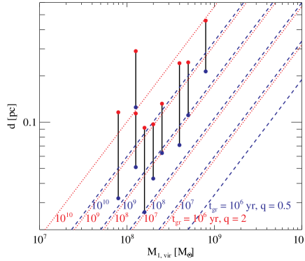
Figure 18.— Virial BH mass (for the active member) vs. estimated binary separations in the BBH model for the nine BBH candidates in Table 3. The red (blue) points denote mass ratio $q=2$ ($q=0.5$). Each solid line connects the two different estimates for the same object. The red dotted (blue dashed) lines are constant orbital decay timescales due to gravitational radiation, $t_{{\rm gr}}$ (Equation (1)), for circular binaries with mass ratio $q=2$ ($q=0.5$). $t_{{\rm gr}}$ is of order the age of the universe at the quasar redshifts for $q$ of order unity (see Section 6.5 for more discussion).

Figure 18 shows the BBH candidates in the $M_{1}$–$d$ plane, using the virial estimate $M_{1}$ for the active BH 1 and the binary separation $d$ as discussed in Section 6.3 assuming mass ratio $q=0.5,~{}2$ and orbital inclination $I=45^{\circ}$ (Table 3). The red dotted (blue dashed) line shows the orbital decay time due to gravitational radiation in a circular binary with a mass ratio $q=2$ ($q=0.5$), which is given by (Peters, 1964)

$$t_{{\rm gr}}=\frac{5}{256}\frac{c^{5}}{G^{3}}\frac{d^{4}}{q(1+q)M_{1}^{3}}~{}.$$ (1)

Most of the purported BBH candidates have GW decay times $t_{{\rm gr}}\gtrsim 10^{9}$ yr (Table 3). $t_{{\rm gr}}$ could be an overestimate for the actual orbital decay time, if other more efficient decay processes (either stellar or gaseous) are at work. For $q\sim 1$, $t_{{\rm gr}}$ is of order the age of the universe at the quasar redshifts. None of the detected systems has short gravitational decay time (e.g., $t_{\rm gr}\ll$ the Hubble time, so that the probability of detecting them is very small). This is reassuring evidence that the BBH interpretation is at least self-consistent.

7. Summary and Future Work

Long-term spectroscopic monitoring of statistical quasar samples is used to test the hypothesis that some of them may contain sub-pc BBHs. The approach is to look for temporal RV shifts of the broad lines to constrain the purported binary orbital motion. In Paper I, we have studied the general quasar population using multiple spectroscopic observations from the SDSS. Here in the second paper in the series, we focus on objects which are pre-selected to have a supposedly higher likelihood of being BBHs. We have selected a sample of 399 quasars from the SDSS DR7 whose broad H$\beta$ lines are significantly (99.7% confidence) offset from the systemic redshift determined from narrow emission lines. The velocity offset has been suggested as evidence for BBHs, but single-epoch spectra cannot rule out alternative scenarios such as accretion disk emitters around single BHs or recoil BHs.

As a pilot program, we have obtained second-epoch optical spectra from MMT/BCS, ARC 3.5 m/DIS, and FLWO 1.5 m/FAST for 50 of the 399 offset-line quasars, separated by $\sim 5$–10 yr (rest frame) from the original SDSS observations. We summarize our main findings in the following.

1. We have adopted a $\chi^{2}$-based cross-correlation method to accurately measure the velocity shifts between two epochs, with particular attention paid to quantifying the uncertainties (Paper I). The velocity shifts have been measured from the broad-line components after subtracting the pseudo-continua and narrow emission lines with reliable spectral decompositions (Shen et al., 2011b) and systematics control (Shen et al., 2013). The velocity-shift zero point has been calibrated using simultaneous observations of the [O III] emission lines. We have detected significant (99% confidence) RV shifts in broad H$\beta$ in 24 of the 50 followup targets and have placed limits on the rest (Section 5.4). For the detected cases, the absolute values of the measured accelerations are $\sim 10$ to $\sim 200$ km s^-1 yr^-1, with a typical measurement uncertainty of $\sim 10$ km s^-1 yr^-1.

2. Following Paper I, we have divided the 24 detections into three categories, which include 9 “BBH candidates”, 5 “BLR variability”, and 10 “ambiguous” cases. For BBH candidates, we require that the measured velocity shift is caused by an overall shift in the bulk velocity, rather than variation in the broad-line profiles. We further require that the velocity shifts independently measured from a second broad line (either broad H$\alpha$ or Mg II) are consistent with those measured from broad H$\beta$.

3. Compared to the general quasar population (i.e., with no significant broad-line velocity offsets) studied in Paper I, our results suggest that the frequency of broad-line shifts in offset quasars is marginally higher on timescales of more than a few years ($\sim$50% $\pm$ 10% for $\Delta t>5$ yr with median velocity shift uncertainty of 50 km s^-1 for offset quasars, compared to $\sim$30% $\pm$ 10% for $\Delta t>5$ yr with median velocity shift uncertainty of 40 km s^-1 for normal quasars), after accounting for differences in time separation and measurement sensitivity (Section 5.1). However, the statistics are poor and the results are consistent with having no difference between the two populations. Offset-broad-line quasars also show larger radial accelerations averaged over a few years than normal quasars (Section 5.2), with an intrinsic width of the acceleration distribution $\sim$30% broader than that of the superior sample of Paper I, although the timescales being probed are very different ($>$5 yr in this work compared to an average of $\sim$1 yr in Paper I) so a fair comparison is difficult.

4. Combining our followup sample with the “superior” sample defined in Paper I, we have found a tentative (Spearman $P_{{\rm null}}\sim 10^{-3}$) anti-correlation between the broad-line velocity offset (both in peak and centroid) in the first-epoch spectra and the acceleration between the first and second epoch (Section 5.3). The velocity offset and acceleration tend to show opposite signs, in the sense that blueshifted (redshifted) broad emission lines in the first-epoch spectra are likely to become less blueshifted (redshifted) in the second-epoch spectra after a few years. However, the correlation is weak and would need to be confirmed with larger samples in future work.

5. We have discussed implications of our results under the BBH hypothesis (Section 6.2). If the velocity offsets and accelerations are due to BBHs, then the observed anti-correlation in the velocity offset and the average acceleration between two epochs can be explained as orbital phase modulation, when the time baseline is a non-negligible fraction of (and is smaller than) the orbital period. The selection of significant broad-line velocity offsets in single-epoch spectra would boost the chance of detecting accelerations after a few years, given fixed measurement accuracy.

6. We have estimated orbital parameters for the nine BBH candidates assuming that the orbits are circular and that only one BH is active (Section 6.4). For binaries with roughly equal BH masses, the estimated binary separations are $\lesssim 0.1$ pc to $\sim 0.5$ pc with orbital periods of a few decades to a few centuries (Table 3). The gravitational radiation decay timescales are of order the age of the universe at the quasar redshifts (Section 6.5). While the models are clearly oversimplified and the BBH hypothesis lacks verification, our results suggest that the binary models provide a viable explanation of the data. If confirmed with future observations, the frequency of the BBH candidates among all quasars would set a lower limit for the space density of sub-pc BBHs at $z\sim 0.5$ as $\sim 2\times 10^{-6}$ Mpc^-3 (for systems with BH masses comparable to those of SDSS quasars, assuming that the duty cycle for BBHs is the same as for single BHs).

This work and Paper I represent a first step toward identifying sub-pc BBHs in quasars and in sorting out the origins for the observed broad emission line velocity offsets. Given that the orbital periods are expected to be a few decades at least (Table 3), detecting a complete binary orbit would be a challenging exercise, but a continuing constant acceleration without changes in the profile shape would already be a strong signature for a BBH. The spectroscopic monitoring work also needs to be extended to quasars with lower luminosities, where our method would be sensitive to systems with a shorter period, at a fixed BH mass (because the expected BLR size would be smaller, thus allowing systems with smaller binary separations). In addition, more observations are needed for a larger sample to confirm the tentative anti-correlation between broad-line offset and acceleration suggested by the pilot study here, and to explore the diversity of BBH candidates. Future followup observations with longer time baselines would effectively mitigate measurement uncertainty for the radial acceleration, similar to the situation measuring stellar proper motions, where the error drops as $T^{-3/2}$ when observing at a steady rate for an interval $T$. For example, spectra taken in summer 2014 would improve the S/N by a factor of $\sim 30$%, and spectra taken in 2016 would improve the S/N by $\sim 60$%. Other future work includes systematic assessment of the quasar and host galaxy properties (e.g., spectral energy distributions; Tanaka & Haiman, 2013; Roedig et al., 2014; Generozov & Haiman, 2014) for offset-broad-line quasars and comparison studies against normal quasars or double-peaked broad-line quasars with extreme velocity offsets, to search for indirect evidence as complementary tests of the BBH hypothesis.

In addition, our pilot followup program has also detected objects with kinematically offset broad emission lines whose offset velocities (and profiles) stay remarkably stable to within a few km s^-1 yr^-1 over many years (rest frame). This is markedly different from the expectation and empirical evidence from observations of double-peaked broad-line objects generally interpreted as disk emitters, and could signal a recoiling BH. More work (e.g., based on photoionization arguments to examine whether the ionizing source is significantly displaced from the galactic core; Bonning et al., 2007; Shields et al., 2009) is needed to examine the possibility of recoiling BHs, which will be the subject of a future paper.

Appendix A Binary Black Hole Model Assumptions

Following Paper I, we consider a BBH on a circular orbit, where only BH 1 (with mass $M_{1}$) is active and powering the observed broad emission lines. The typical size of the BLR around a single BH with mass $M_{1}$ is $R_{{\rm BLR}}\sim 2.7\times 10^{-2}(L/10^{45}{\rm erg\,s}^{-1})^{1/2}$ pc (Shen & Loeb, 2010). The orbital period, LOS velocity and acceleration of the active BH are (Paper I)

$$\begin{split}P&=9.4d^{3/2}_{0.01}M^{-1/2}_{8,{\rm tot}}~{}~{}~{}~{}{\rm yr},\\ V_{1}&=6560\bigg{(}\frac{M_{2}}{M_{{\rm tot}}}\bigg{)}M^{1/2}_{8,{\rm tot}}d^{-1/2}_{0.01}\sin I\sin\phi~{}~{}~{}~{}{\rm km~{}s}^{-1},\\ a_{1}&=4400\bigg{(}\frac{M_{2}}{10^{8}M_{\odot}}\bigg{)}d^{-2}_{0.01}\sin I\cos\phi~{}~{}~{}~{}{\rm km~{}s}^{-1}~{}{\rm yr}^{-1},\end{split}$$ (A1)

where subscripts 1 and 2 refer to BH 1 and 2, respectively, $I$ is the orbital inclination, $d$ is the binary separation, $\phi$ is the orbital phase, $M_{{\rm tot}}\equiv M_{1}+M_{2}$, $M_{8,{\rm tot}}\equiv M_{{\rm tot}}/10^{8}M_{\odot}$, and $d_{0.01}\equiv d/0.01{\rm pc}$.

We have set $V_{1}$ equal to the average of the velocity offsets from the SDSS and followup spectra and determined $a_{1}$ from the difference in these offsets. Assuming values for the orbital inclination $I$ and mass ratio $q\equiv M_{2}/M_{1}$, we can solve the above equations for $d$ and $P$. From the last two relations in Equation (A1), we get a quartic polynomial in $d_{0.01}$:

$$\begin{split}C_{1}d^{4}_{0.01}+C_{2}d_{0.01}-1&=0,\end{split}$$ (A2)

where $C_{1}=(a_{1}/4400~{}{\rm km}~{}{\rm s}^{-1}~{}{\rm yr}^{-1})^{2}(M_{1}/10^{8}M_{\odot})^{-2}q^{-2}(\sin I)^{-2}$ and $C_{2}=(V_{1}/6560~{}{\rm km}~{}{\rm s}^{-1})^{2}q^{-2}(1+q)(M_{1}/10^{8}M_{\odot})^{-1}(\sin I)^{-2}$. The equation always has two real roots (one positive and one negative) and two complex conjugate roots, and we take the real positive root as the solution. The resulting $d$ should at least satisfy $d>R_{{\rm BLR}}$ for the model to be self-consistent. If we further require that the BLR size must be smaller than the Roche radius, the result must satisfy the stronger constraint $d>f^{-1}_{r}R_{{\rm BLR}}$, where $f_{r}$ is the average radius of the Roche lobe in a circular binary system (e.g., Paczynski, 1971):

$$\begin{split}f_{r}&=0.38-0.2\log q,~{}~{}~{}~{}0.05<q<1.88\\ &=0.46224(1+q)^{-1/3},~{}~{}~{}~{}q>1.88.\end{split}$$ (A3)

References

- Abazajian et al. (2009) Abazajian, K. N., et al. 2009, ApJS, 182, 543
- Abt & Levy (1976) Abt, H. A., & Levy, S. G. 1976, ApJS, 30, 273
- Amaro-Seoane et al. (2012) Amaro-Seoane, P., et al. 2012, Classical and Quantum Gravity, 29, 124016
- Baker et al. (2006) Baker, J. G., Centrella, J., Choi, D.-I., Koppitz, M., van Meter, J. R., & Miller, M. C. 2006, ApJ, 653, L93
- Ballo et al. (2004) Ballo, L., Braito, V., Della Ceca, R., Maraschi, L., Tavecchio, F., & Dadina, M. 2004, ApJ, 600, 634
- Begelman et al. (1980) Begelman, M. C., Blandford, R. D., & Rees, M. J. 1980, Nature, 287, 307
- Bentz et al. (2009) Bentz, M. C., Peterson, B. M., Netzer, H., Pogge, R. W., & Vestergaard, M. 2009, ApJ, 697, 160
- Bianchi et al. (2008) Bianchi, S., Chiaberge, M., Piconcelli, E., Guainazzi, M., & Matt, G. 2008, MNRAS, 386, 105
- Blecha et al. (2011) Blecha, L., Cox, T. J., Loeb, A., & Hernquist, L. 2011, MNRAS, 412, 2154
- Bogdanović et al. (2009) Bogdanović, T., Eracleous, M., & Sigurdsson, S. 2009, ApJ, 697, 288
- Bogdanović et al. (2007) Bogdanović, T., Reynolds, C. S., & Miller, M. C. 2007, ApJ, 661, L147
- Bogdanović et al. (2008) Bogdanović, T., Smith, B. D., Sigurdsson, S., & Eracleous, M. 2008, ApJS, 174, 455
- Bon et al. (2012) Bon, E., et al. 2012, ApJ, 759, 118
- Bonning et al. (2007) Bonning, E. W., Shields, G. A., & Salviander, S. 2007, ApJ, 666, L13
- Boroson (2002) Boroson, T. A. 2002, ApJ, 565, 78
- Boroson & Green (1992) Boroson, T. A., & Green, R. F. 1992, ApJS, 80, 109
- Boroson & Lauer (2009) Boroson, T. A., & Lauer, T. R. 2009, Nature, 458, 53
- Boroson & Lauer (2010) —. 2010, AJ, 140, 390
- Burke-Spolaor (2011) Burke-Spolaor, S. 2011, MNRAS, 410, 2113
- Campanelli et al. (2007) Campanelli, M., Lousto, C. O., Zlochower, Y., & Merritt, D. 2007, Physical Review Letters, 98, 231102
- Centrella et al. (2010) Centrella, J., Baker, J. G., Kelly, B. J., & van Meter, J. R. 2010, Reviews of Modern Physics, 82, 3069
- Chapon et al. (2013) Chapon, D., Mayer, L., & Teyssier, R. 2013, MNRAS, 429, 3114
- Chen et al. (1989) Chen, K., Halpern, J. P., & Filippenko, A. V. 1989, ApJ, 339, 742
- Chornock et al. (2010) Chornock, R., et al. 2010, ApJ, 709, L39
- Colpi & Dotti (2011) Colpi, M., & Dotti, M. 2011, Advanced Science Letters, 4, 181
- Comerford et al. (2012) Comerford, J. M., Gerke, B. F., Stern, D., Cooper, M. C., Weiner, B. J., Newman, J. A., Madsen, K., & Barrows, R. S. 2012, ApJ, 753, 42
- Comerford et al. (2009) Comerford, J. M., Griffith, R. L., Gerke, B. F., Cooper, M. C., Newman, J. A., Davis, M., & Stern, D. 2009, ApJ, 702, L82
- Comerford et al. (2011) Comerford, J. M., Pooley, D., Gerke, B. F., & Madejski, G. M. 2011, ApJ, 737, L19
- Corbin & Boroson (1996) Corbin, M. R., & Boroson, T. A. 1996, ApJS, 107, 69
- Decarli et al. (2013) Decarli, R., Dotti, M., Fumagalli, M., Tsalmantza, P., Montuori, C., Lusso, E., Hogg, D. W., & Prochaska, J. X. 2013, MNRAS, 433, 1492
- Dotti et al. (2006) Dotti, M., Colpi, M., & Haardt, F. 2006, MNRAS, 367, 103
- Dotti et al. (2012) Dotti, M., Sesana, A., & Decarli, R. 2012, Advances in Astronomy, 2012
- Dotti et al. (2010) Dotti, M., Volonteri, M., Perego, A., Colpi, M., Ruszkowski, M., & Haardt, F. 2010, MNRAS, 402, 682
- Ebisuzaki et al. (1991) Ebisuzaki, T., Makino, J., & Okumura, S. K. 1991, Nature, 354, 212
- Eracleous (1999) Eracleous, M. 1999, in Astronomical Society of the Pacific Conference Series, Vol. 175, Structure and Kinematics of Quasar Broad Line Regions, ed. C. M. Gaskell, W. N. Brandt, M. Dietrich, D. Dultzin-Hacyan, & M. Eracleous, 163–+
- Eracleous et al. (2012) Eracleous, M., Boroson, T. A., Halpern, J. P., & Liu, J. 2012, ApJS, 201, 23
- Eracleous & Halpern (2003) Eracleous, M., & Halpern, J. P. 2003, ApJ, 599, 886
- Eracleous et al. (1997) Eracleous, M., Halpern, J. P., Gilbert, A. M., Newman, J. A., & Filippenko, A. V. 1997, ApJ, 490, 216
- Eracleous et al. (1995) Eracleous, M., Livio, M., Halpern, J. P., & Storchi-Bergmann, T. 1995, ApJ, 438, 610
- Escala et al. (2005) Escala, A., Larson, R. B., Coppi, P. S., & Mardones, D. 2005, ApJ, 630, 152
- Fabbiano et al. (2011) Fabbiano, G., Wang, J., Elvis, M., & Risaliti, G. 2011, Nature, 477, 431
- Faber et al. (1997) Faber, S. M., et al. 1997, AJ, 114, 1771
- Fabricant et al. (1998) Fabricant, D., Cheimets, P., Caldwell, N., & Geary, J. 1998, PASP, 110, 79
- Fitchett (1983) Fitchett, M. J. 1983, MNRAS, 203, 1049
- Fu et al. (2012) Fu, H., Yan, L., Myers, A. D., Stockton, A., Djorgovski, S. G., Aldering, G., & Rich, J. A. 2012, ApJ, 745, 67
- Fu et al. (2011) Fu, H., et al. 2011, ApJ, 740, L44
- Gaskell (1983) Gaskell, C. M. 1983, in Liege International Astrophysical Colloquia, Vol. 24, Liege International Astrophysical Colloquia, ed. J.-P. Swings, 473–477
- Gaskell (1996) Gaskell, C. M. 1996, ApJ, 464, L107
- Generozov & Haiman (2014) Generozov, A., & Haiman, Z. 2014, ArXiv e-prints 1403.0002
- Gezari et al. (2007) Gezari, S., Halpern, J. P., & Eracleous, M. 2007, ApJS, 169, 167
- Goodrich (1989) Goodrich, R. W. 1989, ApJ, 342, 224
- Gould & Rix (2000) Gould, A., & Rix, H.-W. 2000, ApJ, 532, L29
- Graham (2004) Graham, A. W. 2004, ApJ, 613, L33
- Green et al. (2010) Green, P. J., Myers, A. D., Barkhouse, W. A., Mulchaey, J. S., Bennert, V. N., Cox, T. J., & Aldcroft, T. L. 2010, ApJ, 710, 1578
- Greene et al. (2011) Greene, J. E., Zakamska, N. L., Ho, L. C., & Barth, A. J. 2011, ApJ, 732, 9
- Gültekin et al. (2009) Gültekin, K., et al. 2009, ApJ, 698, 198
- Halpern & Filippenko (1988) Halpern, J. P., & Filippenko, A. V. 1988, Nature, 331, 46
- Hewett & Wild (2010) Hewett, P. C., & Wild, V. 2010, MNRAS, 405, 2302
- Hoffman & Loeb (2007) Hoffman, L., & Loeb, A. 2007, MNRAS, 377, 957
- Hopkins et al. (2008) Hopkins, P. F., Hernquist, L., Cox, T. J., & Kereš, D. 2008, ApJS, 175, 356
- Hughes et al. (1998) Hughes, P. A., Aller, H. D., & Aller, M. F. 1998, ApJ, 503, 662
- Igumenshchev & Abramowicz (1999) Igumenshchev, I. V., & Abramowicz, M. A. 1999, MNRAS, 303, 309
- Jenet et al. (2004) Jenet, F. A., Lommen, A., Larson, S. L., & Wen, L. 2004, ApJ, 606, 799
- Ju et al. (2013) Ju, W., Greene, J. E., Rafikov, R. R., Bickerton, S. J., & Badenes, C. 2013, ApJ, 777, 44
- Katz (1997) Katz, J. I. 1997, ApJ, 478, 527
- Kauffmann & Haehnelt (2000) Kauffmann, G., & Haehnelt, M. 2000, MNRAS, 311, 576
- Khan et al. (2013) Khan, F. M., Holley-Bockelmann, K., Berczik, P., & Just, A. 2013, ApJ, 773, 100
- Komberg (1968) Komberg, B. V. 1968, Soviet Ast., 11, 727
- Komossa et al. (2003) Komossa, S., Burwitz, V., Hasinger, G., Predehl, P., Kaastra, J. S., & Ikebe, Y. 2003, ApJ, 582, L15
- Kormendy et al. (2009) Kormendy, J., Fisher, D. B., Cornell, M. E., & Bender, R. 2009, ApJS, 182, 216
- Koss et al. (2011) Koss, M., et al. 2011, ApJ, 735, L42
- Koss et al. (2012) Koss, M., Mushotzky, R., Treister, E., Veilleux, S., Vasudevan, R., & Trippe, M. 2012, ApJ, 746, L22
- Kulkarni & Loeb (2012) Kulkarni, G., & Loeb, A. 2012, MNRAS, 422, 1306
- Lehto & Valtonen (1996) Lehto, H. J., & Valtonen, M. J. 1996, ApJ, 460, 207
- Lewis et al. (2010) Lewis, K. T., Eracleous, M., & Storchi-Bergmann, T. 2010, ApJS, 187, 416
- Liu et al. (2013) Liu, X., Civano, F., Shen, Y., Green, P., Greene, J. E., & Strauss, M. A. 2013, ApJ, 762, 110
- Liu et al. (2010a) Liu, X., Greene, J. E., Shen, Y., & Strauss, M. A. 2010a, ApJ, 715, L30
- Liu et al. (2011a) Liu, X., Shen, Y., & Strauss, M. A. 2011a, ApJ, 736, L7+
- Liu et al. (2010b) Liu, X., Shen, Y., Strauss, M. A., & Greene, J. E. 2010b, ApJ, 708, 427
- Liu et al. (2011b) Liu, X., Shen, Y., Strauss, M. A., & Hao, L. 2011b, ApJ, 737, 101
- Lodato et al. (2009) Lodato, G., Nayakshin, S., King, A. R., & Pringle, J. E. 2009, MNRAS, 398, 1392
- Loeb (2007) Loeb, A. 2007, Physical Review Letters, 99, 041103
- Loeb (2010) —. 2010, Phys. Rev. D, 81, 047503
- Mayer et al. (2007) Mayer, L., Kazantzidis, S., Madau, P., Colpi, M., Quinn, T., & Wadsley, J. 2007, Science, 316, 1874
- Mazzarella et al. (2012) Mazzarella, J. M., et al. 2012, AJ, 144, 125
- McGurk et al. (2011) McGurk, R. C., Max, C. E., Rosario, D. J., Shields, G. A., Smith, K. L., & Wright, S. A. 2011, ApJ, 738, L2+
- Merritt (2013) Merritt, D. 2013, Dynamics and Evolution of Galactic Nuclei, Princeton Series in Astrophysics (Princeton University Press)
- Merritt & Milosavljević (2005) Merritt, D., & Milosavljević, M. 2005, Living Reviews in Relativity, 8, 8
- Merritt & Poon (2004) Merritt, D., & Poon, M. Y. 2004, ApJ, 606, 788
- Milosavljević & Merritt (2001) Milosavljević, M., & Merritt, D. 2001, ApJ, 563, 34
- Oke (1974) Oke, J. B. 1974, ApJS, 27, 21
- Osterbrock & Pogge (1985) Osterbrock, D. E., & Pogge, R. W. 1985, ApJ, 297, 166
- Osterbrock & Shuder (1982) Osterbrock, D. E., & Shuder, J. M. 1982, ApJS, 49, 149
- Paczynski (1971) Paczynski, B. 1971, Annual Review of Astronomy and Astrophysics, 9, 183
- Peters (1964) Peters, P. C. 1964, Physical Review, 136, 1224
- Peterson et al. (1987) Peterson, B. M., Korista, K. T., & Cota, S. A. 1987, ApJ, 312, L1
- Piconcelli et al. (2010) Piconcelli, E., et al. 2010, ApJ, 722, L147
- Popović (2012) Popović, L. Č. 2012, NewAR, 56, 74
- Preto et al. (2011) Preto, M., Berentzen, I., Berczik, P., & Spurzem, R. 2011, ApJ, 732, L26
- Richards et al. (2002) Richards, G. T., et al. 2002, AJ, 123, 2945
- Rodriguez et al. (2006) Rodriguez, C., Taylor, G. B., Zavala, R. T., Peck, A. B., Pollack, L. K., & Romani, R. W. 2006, ApJ, 646, 49
- Roedig et al. (2014) Roedig, C., Krolik, J. H., & Miller, M. C. 2014, ApJ, 785, 115
- Roos (1981) Roos, N. 1981, A&A, 104, 218
- Schneider et al. (2010) Schneider, D. P., et al. 2010, AJ, 139, 2360
- Sergeev et al. (2007) Sergeev, S. G., Doroshenko, V. T., Dzyuba, S. A., Peterson, B. M., Pogge, R. W., & Pronik, V. I. 2007, ApJ, 668, 708
- Sesana (2007) Sesana, A. 2007, MNRAS, 382, L6
- Shapovalova et al. (2001) Shapovalova, A. I., et al. 2001, A&A, 376, 775
- Shapovalova et al. (2004) —. 2004, A&A, 422, 925
- Shapovalova et al. (2010) Shapovalova, A. I., Popović, L. Č., Burenkov, A. N., Chavushyan, V. H., Ilić, D., Kovačević, A., Bochkarev, N. G., & León-Tavares, J. 2010, A&A, 509, A106
- Shen (2009) Shen, Y. 2009, ApJ, 704, 89
- Shen (2013) —. 2013, Bulletin of the Astronomical Society of India, 41, 61
- Shen et al. (2008) Shen, Y., Greene, J. E., Strauss, M. A., Richards, G. T., & Schneider, D. P. 2008, ApJ, 680, 169
- Shen et al. (2010) Shen, Y., et al. 2010, ApJ, 719, 1693
- Shen et al. (2011a) Shen, Y., Liu, X., Greene, J. E., & Strauss, M. A. 2011a, ApJ, 735, 48
- Shen et al. (2013) Shen, Y., Liu, X., Loeb, A., & Tremaine, S. 2013, ApJ, 775, 49 (Paper I)
- Shen & Loeb (2010) Shen, Y., & Loeb, A. 2010, ApJ, 725, 249
- Shen et al. (2011b) Shen, Y., et al. 2011b, ApJS, 194, 45
- Shields et al. (2009) Shields, G. A., et al. 2009, ApJ, 707, 936
- Sillanpaa et al. (1988) Sillanpaa, A., Haarala, S., Valtonen, M. J., Sundelius, B., & Byrd, G. G. 1988, ApJ, 325, 628
- Sillanpaa et al. (1996) Sillanpaa, A., et al. 1996, A&A, 305, L17
- Smith et al. (2010) Smith, K. L., Shields, G. A., Bonning, E. W., McMullen, C. C., Rosario, D. J., & Salviander, S. 2010, ApJ, 716, 866
- Stoughton et al. (2002) Stoughton, C., et al. 2002, AJ, 123, 485
- Strateva et al. (2003) Strateva, I. V., et al. 2003, AJ, 126, 1720
- Sudou et al. (2003) Sudou, H., Iguchi, S., Murata, Y., & Taniguchi, Y. 2003, Science, 300, 1263
- Tanaka & Haiman (2013) Tanaka, T. L., & Haiman, Z. 2013, Classical and Quantum Gravity, 30, 224012
- Thorne & Braginskii (1976) Thorne, K. S., & Braginskii, V. B. 1976, ApJ, 204, L1
- Tody (1986) Tody, D. 1986, in Society of Photo-Optical Instrumentation Engineers (SPIE) Conference Series, ed. D. L. Crawford, Vol. 627, 733
- Tremaine et al. (2014) Tremaine, S., Shen, Y., Liu, X., & Loeb, A. 2014, ArXiv e-prints 1406.2468
- Trias & Sintes (2008) Trias, M., & Sintes, A. M. 2008, Phys. Rev. D, 77, 024030
- Tsalmantza et al. (2011) Tsalmantza, P., Decarli, R., Dotti, M., & Hogg, D. W. 2011, ApJ, 738, 20
- Valtaoja et al. (2000) Valtaoja, E., Teräsranta, H., Tornikoski, M., Sillanpää, A., Aller, M. F., Aller, H. D., & Hughes, P. A. 2000, ApJ, 531, 744
- Valtonen et al. (2008) Valtonen, M. J., et al. 2008, Nature, 452, 851
- Van Wassenhove et al. (2012) Van Wassenhove, S., Volonteri, M., Mayer, L., Dotti, M., Bellovary, J., & Callegari, S. 2012, ApJ, 748, L7
- Vasiliev et al. (2014) Vasiliev, E., Antonini, F., & Merritt, D. 2014, ApJ, 785, 163
- Villata et al. (1998) Villata, M., Raiteri, C. M., Sillanpaa, A., & Takalo, L. O. 1998, MNRAS, 293, L13
- Villforth et al. (2010) Villforth, C., et al. 2010, MNRAS, 402, 2087
- Volonteri et al. (2003) Volonteri, M., Haardt, F., & Madau, P. 2003, ApJ, 582, 559
- Volonteri et al. (2009) Volonteri, M., Miller, J. M., & Dotti, M. 2009, ApJ, 703, L86
- Wang et al. (2009) Wang, J., Chen, Y., Hu, C., Mao, W., Zhang, S., & Bian, W. 2009, ApJ, 705, L76
- Wyithe & Loeb (2003) Wyithe, J. S. B., & Loeb, A. 2003, ApJ, 595, 614
- York et al. (2000) York, D. G., et al. 2000, AJ, 120, 1579
- Yu (2002) Yu, Q. 2002, MNRAS, 331, 935
- Yu et al. (2011) Yu, Q., Lu, Y., Mohayaee, R., & Colin, J. 2011, ApJ, 738, 92
- Zamfir et al. (2010) Zamfir, S., Sulentic, J. W., Marziani, P., & Dultzin, D. 2010, MNRAS, 403, 1759
- Zheng & Sulentic (1990) Zheng, W., & Sulentic, J. W. 1990, ApJ, 350, 512