On the limiting behavior of parameter-dependent network centrality measures

Abstract

We consider a broad class of walk-based, parameterized node centrality measures for network analysis. These measures are expressed in terms of functions of the adjacency matrix and generalize various well-known centrality indices, including Katz and subgraph centrality. We show that the parameter can be “tuned” to interpolate between degree and eigenvector centrality, which appear as limiting cases. Our analysis helps explain certain correlations often observed between the rankings obtained using different centrality measures, and provides some guidance for the tuning of parameters. We also highlight the roles played by the spectral gap of the adjacency matrix and by the number of triangles in the network. Our analysis covers both undirected and directed networks, including weighted ones. A brief discussion of PageRank is also given.

Abstract

This document contains details of numerical experiments performed to illustrate the theoretical results presented in our accompanying paper.

1 Introduction

The mathematical and computational study of complex networks has experienced tremendous growth in recent years. A wide variety of highly interconnected systems, both in nature and in the man-made world of technology, can be modeled in terms of networks. Network models are now commonplace not only in the “hard” sciences but also in economics, finance, anthropology, urban studies, and even in the humanities. As more and more data has become available, the need for tools to analyze these networks has increased and a new field of Network Science has come of age [1, 17, 24, 47].

Since graphs, which are abstract models of real-world networks, can be described in terms of matrices, it comes as no surprise that linear algebra plays an important role in network analysis. Many problems in this area require the solution of linear systems, the computation of eigenvalues and eigenvectors, and the evaluation of matrix functions. Also, the study of dynamical processes on graphs gives rise to systems of differential and difference equations posed on graphs [2]; the behavior of the solution as a function of time is strongly influenced by the structure (topology) of the underlying graph, which in turn is reflected in the spectral properties of matrices associated with the graph [6].

One of the most basic questions about network structure is the identification of the “important” nodes in a network. Examples include essential proteins in Protein-Protein Interaction Networks, keystone species in ecological networks, authoritative web pages on the World Wide Web, influential authors in scientific collaboration networks, leading actors in the Internet Movie Database, and so forth; see, e.g., [24, 46] for details and many additional examples. When the network being examined is very small (say, on the order of 10 nodes), this determination of importance can often be done visually, but as networks increase in size and complexity, visual analysis becomes impossible. Instead, computational measures of node importance, called centrality measures, are used to rank the nodes in a network. There are many different centrality measures in use; see, for example, [13, 24, 40, 47] for extensive treatments of centrality and discussion of different ranking methods. Many authors, however, have noted that different centrality measures often provide rankings that are highly correlated, at least when attention is restricted to the most highly ranked nodes; see. e.g., [21, 32, 41, 45], as well as the results in [5].

In this paper we analyze the relationship between degree centrality, eigenvector centrality, and various centrality measures based on the diagonal entries (for undirected graphs) and row sums of certain (analytic) functions of the adjacency matrix of the graph. These measures contain as special cases the well-known Katz centrality, subgraph centrality, total communicability, and other centrality measures which depend on a tuneable parameter. We also include a brief discussion of PageRank [48]. We point out that Kleinberg’s HITS algorithm [37], as a type of eigenvector centrality, is covered by our analysis, as is the extension of subgraph centrality to digraphs given in [4].

As mentioned, there are a number of other ranking methods in use, yet in this paper we limit ourselves to considering centrality measures based on functions of the adjacency matrix, in addition to degree and eigenvector centrality. The choice of which of the many centrality measures to study and why is something that must be considered carefully; see the discussion in [15]. In this paper we focus our attention on centrality measures that have been widely tested and that can be expressed in terms of linear algebra (more specifically, in terms of the adjacency matrix of the network). We additionally restrict our scope to centrality measures that we can demonstrate (mathematically) to be related to one other. Hence, we did not include in our analysis two popular centrality measures, betweenness centrality [30] and closeness centrality [31], which do not appear to admit a simple expression in terms of the adjacency matrix. Our results help explain the correlations often observed between the rankings produced by different centrality measures, and may be useful in tuning parameters when performing centrality calculations.

The paper is organized as follows. Sections 2 and 3 contain background information on graphs and centrality measures. In section 4 we describe the general class of functional centrality measures considered in this paper and present some technical lemmas on power series needed for our analysis. In section 5 we state and prove our main results, which show that degree and eigenvector centrality are limiting cases of the parameterized ones. Section 6 contains a brief discussion of the limiting behavior of PageRank and related techniques. In section 7 we provide an interpretation of our results in terms of graph walks and discuss the role played by the spectral gap and by triangles in the network. Related work is briefly reviewed in section 8. A short summary of numerical experiments aimed at illustrating the theory is given in section 9 (the details of the experiments can be found in the Supplementary Materials accompanying this paper). Conclusions are given in section 10.

2 Background and definitions

In this section we recall some basic concepts from graph theory that will be used in the rest of the paper. A more complete overview can be found, e.g., in [20]. For ease of exposition only unweighted and loopless graphs are considered in this section, but nearly all of our results admit a straightforward generalization to graphs with (positive) edge weights, and several of the results also apply in the presence of loops; see the end of section 5, as well as section 6.

A directed graph, or digraph, $G=(V,E)$ is defined by a set of $n$ nodes (also referred to as vertices) $V$ and a set of edges $E=\{(i,j)\,|\,i,j\in V\}$. Note that, in general, $(i,j)\in E$ does not imply $(j,i)\in E$. When this happens, $G$ is undirected and the edges are formed by unordered pairs of vertices. The out-degree of a vertex $i$, denoted by $d_{i}^{out}$, is given by the number of edges with $i$ as the starting node, i.e., the number of edges in $E$ of the form $(i,k)$. Similarly, the in-degree of node $i$ is the number $d_{i}^{in}$ of edges of the form $(k,i)$. If $G$ is undirected then $d_{i}^{out}=d_{i}^{in}=d_{i}$, the degree of node $i$.

A walk of length $k$ in $G$ is a list of nodes $i_{1},i_{2},\ldots i_{k},i_{k+1}$ such that for all $1\leq l\leq k$, there is a (directed) edge between $i_{l}$ and $i_{l+1}$. A closed walk is a walk where $i_{1}=i_{k+1}$. A path is a walk with no repeated nodes, and a cycle is a closed walk with no repeated nodes except for the first and the last one. A graph is simple if it has no loops (edges from a node $i$ to itself), no multiple edges, and unweighted edges. An undirected graph is connected if there exists a path between every pair of nodes. A directed graph is strongly connected if there exists a directed path between every pair of nodes.

Every graph $G$ can be represented as a matrix through the use of an adjacency matrix $A=(a_{ij})$ with

$$a_{ij}=\left\{\begin{array}[]{ll}1,&\textnormal{ if }(i,j)\textnormal{ is an edge in }G,\\ 0,&\textnormal{ else. }\end{array}\right.$$

If $G$ is a simple, undirected graph, $A$ is binary and symmetric with zeros along the main diagonal. In this case, the eigenvalues of $A$ will be real. We label the eigenvalues of $A$ in non-increasing order: $\lambda_{1}\geq\lambda_{2}\geq\ldots\geq\lambda_{n}.$ If $G$ is connected, then $\lambda_{1}>\lambda_{2}$ by the Perron-Frobenius theorem [44, page 673]. Since $A$ is a symmetric, real-valued matrix, we can decompose $A$ into $A=Q\Lambda Q^{T}$ where $\Lambda={\rm diag}(\lambda_{1},\lambda_{2},\ldots,\lambda_{n})$ with $\lambda_{1}>\lambda_{2}\geq\ldots\geq\lambda_{n}$, $Q=[{\bf q}_{1},{\bf q}_{2},\ldots,{\bf q}_{n}]$ is orthogonal, and ${\bf q}_{i}$ is the eigenvector associated with $\lambda_{i}$. The dominant eigenvector, ${\bf q}_{1}$, can be chosen to have positive entries when $G$ is connected: we write this ${\bf q}_{1}>{\bf 0}$.

If $G$ is a strongly connected digraph, its adjacency matrix $A$ is irreducible, and conversely. Let $\rho(A)=r$ be the spectral radius of $A$. Then, again by the Perron-Frobenius theorem, $\lambda_{1}=r$ is a simple eigenvalue of $A$ and both the left and right eigenvectors of $A$ associated with $\lambda_{1}$ can be chosen to be positive. If $G$ is also diagonalizable, then there exists an invertible matrix $X$ such that $A=X\Lambda X^{-1}$ where $\Lambda={\rm diag}(\lambda_{1},\lambda_{2},\ldots,\lambda_{n})$ with $\lambda_{1}\geq|\lambda_{i}|$ for $2\leq i\leq n$, $X=[{\bf x}_{1},{\bf x}_{2},\ldots,{\bf x}_{n}]$, and $(X^{-1})^{T}=[{\bf y}_{1},{\bf y}_{2},\ldots,{\bf y}_{n}]$. The left eigenvector associated with $\lambda_{i}$ is ${\bf y}_{i}$ and the right eigenvector associated with $\lambda_{i}$ is ${\bf x}_{i}$. In the case where $G$ is not diagonalizable, $A$ can be decomposed using the Jordan canonical form:

$$A=XJX^{-1}=X\left(\begin{array}[]{cc}\lambda_{1}&{\bf 0}\\ {\bf 0}&\hat{J}\\ \end{array}\right)X^{-1}\,,$$

where $J$ is the Jordan matrix of $A$, except that we place the $1\times 1$ block corresponding to $\lambda_{1}$ first for notational convenience. The first column ${\bf x}_{1}$ of $X$ is the dominant right eigenvector of $A$ and the first column ${\bf y}_{1}$ of $X^{-T}$ is the dominant left eigenvector of $A$ (equivalently, the dominant right eigenvector of $A^{T}$).

Throughout the paper, $I$ denotes the $n\times n$ identity matrix.

3 Node centrality

As we discussed in the Introduction, many measures of node centrality have been developed and used over the years. In this section we review and motivate several centrality measures to be analyzed in the rest of the paper.

3.1 Some common centrality measures

Some of the most common measures include degree centrality, eigenvector centrality [9], PageRank [48], betweenness centrality [12, 30], Katz centrality [36], and subgraph centrality [26, 27]. More recently, total communicability has been introduced as a centrality measure [5]. A node is deemed “important” according to a given centrality index if the corresponding value of the index is high relative to that of other nodes.

Most of these measures are applicable to both undirected and directed graphs. In the directed case, however, each node can play two roles: sink and source, or receiver and broadcaster, since a node in general can be both a starting point and an arrival point for directed edges. This has led to the notion of hubs and authorities in a network, with hubs being nodes with a high broadcast centrality index and authorities being nodes with a high receive centrality index. For the types of indices considered in this paper, broadcast centrality measures correspond to quantities computed from the adjacency matrix $A$, whereas authority centrality measures correspond to the same quantities computed from the transpose $A^{T}$ of the adjacency matrix. When the graph is undirected, $A=A^{T}$ and the broadcast and receive centrality scores of each node coincide.

Examples of (broadcast) centrality measures are:

• out-degree centrality: $d_{i}^{out}:=[A{\bf 1}]_{i}$;

• (right) eigenvector centrality: $C_{ev}(i):={\bf e}_{i}^{T}{\bf q}_{1}=q_{1}(i)$, where ${\bf q}_{1}$ is the dominant (right) eigenvector of $A$;

• exponential subgraph centrality: $SC_{i}(\beta):=[{\rm e}^{\beta A}]_{ii}$;

• resolvent subgraph centrality: $RC_{i}(\alpha):=[(I-\alpha A)^{-1}]_{ii}$,

• total communicability: $TC_{i}(\beta):=[{\rm e}^{\beta A}{\bf 1}]_{i}={\bf e}_{i}^{T}{\rm e}^{\beta A}{\bf 1}$;

• Katz centrality: $K_{i}(\alpha):=[(I-\alpha A)^{-1}{\bf 1}]_{i}={\bf e}_{i}^{T}(I-\alpha A)^{-1}{\bf 1}$.

Here ${\bf e}_{i}$ is the $i$th standard basis vector, ${\bf 1}$ is the vector of all ones, $0<\alpha<\frac{1}{\lambda_{1}}$ (see below), and $\beta>0$. We note that the vector of all ones is sometimes replaced by a preference vector $\bf v$ with positive entries; for instance, ${\bf v}={\bf d}:=A{\bf 1}$ (the vector of node out-degrees).

Replacing $A$ with $A^{T}$ in the definitions above we obtain the corresponding authority measures. Thus, out-degree centrality becomes in-degree centrality, right eigenvector centrality becomes left eigenvector centrality, and row sums are replaced by column sums when computing the total communicability centrality. Note, however, that the exponential and resolvent subgraph centralities are unchanged when replacing $A$ with $A^{T}$, since $f(A^{T})=f(A)^{T}$ for any matrix function [34, Theorem 1.13]. Hence, measures based on the diagonal entries cannot differentiate between the two roles a node can play in a directed network, and for this reason they are mostly used in the undirected case only (but see [4] for an adaptation of subgraph centrality to digraphs).

Often, the value $\beta=1$ is used in the calculation of exponential subgraph centrality and total communicability. The parameter $\beta$ can be interpreted as an inverse temperature and has been used to model the effects of external disturbances on the network. As $\beta\to 0+$, the “temperature” of the environment surrounding the network increases, corresponding to more intense external disturbances. Conversely, as $\beta\to\infty$, the temperature goes to 0 and the network “freezes.” We refer the reader to [25] for an extensive discussion and applications of these physical analogies.

3.2 Justification in terms of graph walks

The justification behind using the (scaled) matrix exponential to compute centrality measures can be seen by considering the power series expansion of ${\rm e}^{\beta A}$:

$${\rm e}^{\beta A}=I+\beta A+\frac{(\beta A)^{2}}{2!}+\cdots+\frac{(\beta A)^{k}}{k!}+\cdots=\sum_{k=0}^{\infty}\frac{(\beta A)^{k}}{k!}.$$ (1)

It is well-known that given an adjacency matrix $A$ of an unweighted network, $[A^{k}]_{ij}$ counts the total number of walks of length $k$ between nodes $i$ and $j$. Thus $SC_{i}(\beta)=[{\rm e}^{\beta A}]_{ii}$, the exponential subgraph centrality of node $i$, counts the total number of closed walks in the network which are centered at node $i$, weighing walks of length $k$ by a factor of $\frac{\beta^{k}}{k!}$. Unlike degree, which is a purely local index, subgraph centrality takes into account the short, medium and long range influence of all nodes on a given node (assuming $G$ is strongly connected). Assigning decreasing weights to longer walks ensures the convergence of the series (1) while guaranteeing that short-range interactions are given more weight than long-range ones [27].

Total communicability is closely related to subgraph centrality. This measure also counts the number of walks starting at node $i$, scaling walks of length $k$ by $\frac{\beta^{k}}{k!}$. However, rather than just counting closed walks, total communicability counts all walks between node $i$ and every node in the network. The name stems from the fact that $TC_{i}(\beta)=\sum_{j=1}^{n}C_{ij}(\beta)$ where $C_{ij}(\beta):=[{\rm e}^{\beta A}]_{ij}$, the communicability between nodes $i$ and $j$, is a measure of how “easy” it is to exchange a message between nodes $i$ and $j$ over the network; see [25] for details. Although subgraph centrality and total communicability are clearly related, they do not always provide the same ranking of the nodes. Furthermore, unlike subgraph centrality, total communicability can distinguish between the two roles a node can play in a directed network. More information about the relation between the two measures can be found in [5].

The matrix resolvent $(I-\alpha A)^{-1}$ was first used to rank nodes in a network in the early 1950s, when Katz used the column sums to calculate node importance [36]. Since then, the diagonal values have also been used as a centrality measure, see [26]. The resolvent subgraph centrality score of node $i$ is given by $[(I-\alpha A)^{-1}]_{ii}$ and the Katz centrality score is given by either $[(I-\alpha A)^{-1}{\bf 1}]_{i}$ or $[(I-\alpha A^{T})^{-1}{\bf 1}]_{i}$, depending on whether hub or authority scores are desired. As mentioned, $\bf 1$ may be replaced by an arbitary (positive) preference vector, $\bf v$.

As when using the matrix exponential, these resolvent-based centrality measures count the number of walks in the network, penalizing longer walks. This can be seen by considering the Neumann series expansion of $(I-\alpha A)^{-1}$, valid for $0<\alpha<\frac{1}{\lambda_{1}}$:

$$(I-\alpha A)^{-1}=I+\alpha A+\alpha^{2}A^{2}+\cdots+\alpha^{k}A^{k}+\cdots=\sum_{k=0}^{\infty}\alpha^{k}A^{k}.$$ (2)

The resolvent subgraph centrality of node $i$, $[(I-\alpha A)^{-1}]_{ii}$, counts the total number of closed walks in the network which are centered at node $i$, weighing walks of length $k$ by $\alpha^{k}$. Similarly, the Katz centrality of node $i$ counts all walks beginning at node $i$, penalizing the contribution of walks of length $k$ by $\alpha^{k}$. The bounds on $\alpha$ ($0<\alpha<\frac{1}{\lambda_{1}}$) ensure that the matrix $I-\alpha A$ is invertible and that the power series in (2) converges to its inverse. The bounds on $\alpha$ also force $(I-\alpha A)^{-1}$ to be nonnegative, as $I-\alpha A$ is a nonsingular $M$-matrix. Hence, both the diagonal entries and the row/column sums of $(I-\alpha A)^{-1}$ are positive and can thus be used for ranking purposes.

4 A general class of functional centrality measures

In this section we establish precise conditions that a matrix function $f(A)$, where $A$ is the adjacency matrix of a network, should satisfy in order to be used in the definition of walk-based centrality measures. We consider in particular analytic functions expressed by power series, with a focus on issues like convergence, positivity, and dependence on a tuneable parameter $t>0$. We also formulate some auxiliary results on power series that will be crucial for the analysis to follow. For an introduction to the properties of analytic functions see, e.g., [42].

4.1 Admissible matrix functions

As discussed in subsection 3.2, walk-based centrality measures (such as Katz or subgraph centrality) lead to power series expansions in the (scaled) adjacency matrix of the network. While exponential- and resolvent-based centrality measures are especially natural (and well-studied), there are a priori infinitely many other matrix functions which could be used [49, 26]. Not every function of the adjacency matrix, however, is suitable for the purpose of defining centrality measures, and some restrictions must be imposed.

A first obvious condition is that the function should be defined by a power series with real coefficients. This guarantees that $f(z)$ takes real values when the argument is real, and that $f(A)$ has real entries for any real $A$. In [49] (see also [26]), the authors proposed to consider only analytic functions admitting a Maclaurin series expansion of the form

$$f(z)=\sum_{k=0}^{\infty}c_{k}z^{k},\quad c_{k}\geq 0\quad{\rm for}\quad k\geq 0\,.$$ (3)

This ensures that $f(A)$ will be nonnegative for any adjacency matrix $A$. In [26] it is further required that $c_{k}>0$ for all $k=1,2,\ldots,n-1$, so as to guarantee that $[f(A)]_{ij}>0$ for all $i\neq j$ whenever the network is (strongly) connected. Although not explicitly stated in [26], it is clear that if one wants all the walks (of any length) in $G$ to make a positive contribution to a centrality measure based on $f$, then one should impose the more restrictive condition $c_{k}>0$ for all $k\geq 0$. Note that $c_{0}$ plays no significant role, since it’s just a constant value added to all the diagonal entries of $f(A)$ and therefore does not affect the rankings. However, imposing $c_{0}>0$ guarantees that all entries of $f(A)$ are positive, and leads to simpler formulas. Another tacit assumption in [26] is that only power series with a positive radius of convergence should be considered.

In the following, we will denote by $\cal P$ the class of analytic functions that can be expressed as sums of power series with strictly positive coefficients on some open neighborhood of $0$. We note in passing that $\cal P$ forms a positive cone in function space, i.e., $\cal P$ is closed under linear combinations with positive coefficients.

Clearly, given an arbitrary adjacency matrix $A$, the matrix function $f(A)$, with $f\in{\cal P}$, need not be defined; ndeed, $f$ must be defined on the spectrum of $A$ [34]. If $f$ is entire (i.e., analytic in the whole complex plane, like the exponential function) then $f(A)$ will always be defined, but this is not the case of functions with singularities, such as the resolvent. However, this difficulty can be easily circumvented by introducing a (scaling) parameter $t$, and by considering for a given $A$ the parameterized matrix function $g(t,A):=f(tA)$ only for values of $t$ such that the power series

$$f(tA)=c_{0}I+c_{1}tA+c_{2}t^{2}A^{2}+\cdots=\sum_{k=0}^{\infty}c_{k}t^{k}A^{k}$$

is convergent; that is, such that $|t\lambda_{1}(A)|<R_{f}$, where $R_{f}$ denotes the radius of convergence of the power series representing $f$. In practice, for the purposes of this paper, we will limit ourselves to positive values of $t$ in order to guarantee that $f(tA)$ is entry-wise positive, as required by the definition of a centrality index. We summarize our discussion so far in the following lemma.

Lemma 1.

Let $\cal P$ be the class of all analytic functions that can be expressed by a Maclaurin series with strictly positive coefficients in an open disk centered at $0$. Given an irreducible adjacency matrix $A$ and a function $f\in\cal P$ with radius of convergence $R_{f}>0$, let $t^{*}=R_{f}/\lambda_{1}(A)$. Then $f(tA)$ is defined and strictly positive for all $t\in(0,t^{*})$. If $f$ is entire, then one can take $t^{*}=\infty$.

Restriction of $f$ to the class $\cal P$ and use of a positive parameter $t$, which will depend on $A$ and $f$ in case $f$ is not entire, allows one to define the notion of $f$-centrality (as well as $f$-communicability, $f$-betweenness, and so forth, see [26]). Exponential subgraph centrality (with $t=\beta$) is an example of an entire function (hence all positive values of $\beta$ are feasible), while resolvent subgraph centrality (with $t=\alpha$) exemplifies the situation where the parameter must be restricted to a finite interval, in this case $(0,\frac{1}{\lambda_{1}(A)})$ (since the geometric series $1+x+x^{2}+\cdots$ has radius of convergence $R_{f}=1$).

We consider now two subclasses of the class $\cal P$ previously introduced. We let ${\cal P}_{\infty}$ denote the set of all power series in $\cal P$ with radius of convergence $R_{f}=\infty$, and with ${\cal P}^{\infty}$ the set of all power series with finite radius of convergence $R_{f}$ such that

$$\sum_{k=0}^{\infty}c_{k}R_{f}^{k}=\lim_{t\to 1^{-}}\sum_{k=0}^{\infty}c_{k}t^{k}R_{f}^{k}=\infty$$ (4)

(we note that the first equality above follows from Abel’s Theorem [42, p. 229]). The exponential and the resolvent are representative of functions in ${\cal P}_{\infty}$ and ${\cal P}^{\infty}$, respectively. It is worth emphasizing that together, ${\cal P}_{\infty}$ and ${\cal P}^{\infty}$ do not exhaust the class $\cal P$. For example, the function $f(z)=\sum_{k=0}^{\infty}\frac{z^{k}}{k^{2}}$ is in $\cal P$, but it is not in ${\cal P}_{\infty}$ (since its radius of convergence is $R_{f}=1$) or in ${\cal P}^{\infty}$, since

$$\lim_{t\to 1^{-}}\sum_{k=0}^{\infty}\frac{t^{k}R_{f}^{k}}{k^{2}}=\sum_{k=0}^{\infty}\frac{1}{k^{2}}=\frac{\pi^{2}}{6}<\infty.$$

In section 5 we will analyze centrality measures based on functions $f$ in ${\cal P}$ and its subclasses, ${\cal P}_{\infty}$ and ${\cal P}^{\infty}$.

4.2 Asymptotic behavior of the ratio of two power series

In our study of the limiting behavior of parameter-dependent functional centrality measures we will need to investigate the asymptotic behavior of the ratio of two power series with positive coefficients. The following technical lemmas will be crucial for our analysis.

Lemma 2.

Let the power series $\sum_{k=0}^{\infty}a_{k}t^{k}$, $\sum_{k=0}^{\infty}b_{k}t^{k}$ have positive real coefficients and be convergent for all $t\geq 0$. If ${\displaystyle{\lim_{k\to\infty}\frac{a_{k}}{b_{k}}=0}}$, then

$$\lim_{t\to\infty}\frac{\sum_{k=0}^{\infty}a_{k}t^{k}}{\sum_{k=0}^{\infty}b_{k}t^{k}}=0\,.$$

Proof.

Let $\varepsilon>0$ be arbitrary and let $N>0$ be such that $\frac{a_{k}}{b_{k}}<\varepsilon$ for all $k>N$. Also, let $g(t)=\sum_{k=0}^{\infty}a_{k}t^{k}$ and $h(t)=\sum_{k=0}^{\infty}b_{k}t^{k}$. We have

$$\frac{g(t)}{h(t)}=\frac{T_{N}^{g}(t)+g_{1}(t)}{T_{N}^{h}(t)+h_{1}(t)}=\frac{T_{N}^{g}(t)}{T_{N}^{h}(t)+h_{1}(t)}+\frac{g_{1}(t)}{T_{N}^{h}(t)+h_{1}(t)},$$ (5)

with $T_{N}^{g}(t)=\sum_{k=0}^{N}a_{k}t^{k}$, $T_{N}^{h}(t)=\sum_{k=0}^{N}b_{k}t^{k}$ and $g_{1}(t)$, $h_{1}(t)$ being the tails of the corresponding series. The first term on the right-hand side of (5) manifestly tends to zero as $t\to\infty$. The second term is clearly bounded above by $g_{1}(t)/h_{1}(t)$. The result then follows from

$$g_{1}(t)=\sum_{k=N+1}^{\infty}a_{k}t^{k}=\sum_{k=N+1}^{\infty}\left(\frac{a_{k}}{b_{k}}\right)b_{k}t^{k}<\varepsilon\,h_{1}(t)$$

and the fact that $\varepsilon$ is arbitrary. ∎

Lemma 3.

Let $\lambda_{1},\lambda_{2},\ldots,\lambda_{n}\in{\mathbb{C}}$ be given, with $\lambda_{1}>|\lambda_{2}|\geq\cdots\geq|\lambda_{n}|$, and let $f\in{\cal P}_{\infty}\cup{\cal P}^{\infty}$ be defined at these points. Then

$$\lim_{t\to t^{*}-}\frac{t^{j}f^{(j)}(t\lambda_{i})}{f(t\lambda_{1})}=0,\quad{\rm for}\quad j=0,1,\ldots,\quad i=2,\ldots n\,,$$ (6)

where $t^{*}=R_{f}/\lambda_{1}$ and $R_{f}$ is the radius of convergence of the series defining $f$ around $0$ (finite or infinite according to whether $f\in{\cal P}^{\infty}$ or $f\in{\cal P}_{\infty}$, respectively).

Proof.

Consider first the case $t^{*}<\infty$. In this case the assumption that $f\in{\cal P}^{\infty}$ guarantees (cf. (4)) that the denominator of (6) tends to infinity, whereas the numerator remains finite for all $i\neq 1$ and all $j$. Indeed, each derivative $f^{(j)}(z)$ of $f(z)$ can be expressed by a power series having the same radius of convergence as the power series expressing $f(z)$. Since each $t^{*}\lambda_{i}$ (with $i\neq 1$) falls inside the circle of convergence, we have $|f^{(j)}(t^{*}\lambda_{i})|<\infty$ for each $j\geq 0$, hence (6).

Next, we consider the case where $t^{*}=\infty$. Let $i\neq 1$ and assume $\lambda_{i}\neq 0$ (the result is trivial for $\lambda_{i}=0$). Since $f$ is entire, so are all its derivatives and moreover

$$|f^{(j)}(t\lambda_{i})|=\left|\sum_{k=0}^{\infty}(k+j)^{\underline{j}}\,c_{k+j}t^{k}\lambda_{i}^{k}\right|\leq\sum_{k=0}^{\infty}(k+j)^{\underline{j}}\,c_{k+j}t^{k}|\lambda_{i}|^{k}<\infty\,,$$ (7)

where we have used the (standard) notation $(k+j)^{\underline{j}}=(k+j)(k+j-1)\cdots(k+1)$ (with the convention $k^{\underline{0}}=1$). Now let $a_{k}=(k+j)^{\underline{j}}\,c_{k+j}\lambda_{i}^{k}$ be the coefficient of $t^{k}$ in the power series expansion of $t^{j}f^{(j)}(t\lambda_{i})$ and let $b_{k}=c_{k}\lambda_{i}^{k}$ be the coefficient of $t^{k}$ in the power series expansion of $f(t\lambda_{1})$, then

$$\frac{a_{k}}{b_{k}}=(k+j)^{\underline{j}}\left(\frac{|\lambda_{i}|}{\lambda_{1}}\right)^{k},\quad{\rm for\,\,all}\quad k\geq j.$$ (8)

Since exponential decay trumps polynomial growth, we conclude that the expression in (8) tends to zero as $k\to\infty$. Using Lemma 2 we obtain the desired conclusion. ∎

As we will see in the next section, the limit (6) with $j=0$ will be instrumental in our analysis of undirected networks, while the general case is needed for the analysis of directed networks.

5 Limiting behavior of parameterized centrality measures

One difficulty in measuring the “importance” of a node in a network is that it is not always clear which of the many centrality measures should be used. Additionally, it is not clear a priori when two centrality measures will give similar node rankings on a given network. When using parameter-dependent indices, such as Katz, exponential, or resolvent-based subgraph centrality, the necessity of choosing the value of the parameter adds another layer of difficulty. For instance, it is well known that using different choices of $\alpha$ and $\beta$ in Katz and subgraph centrality will generally produce different centrality scores and can lead to different node rankings. However, experimentally, it has been observed that different centrality measures often provide rankings that are highly correlated [5, 21, 32, 41, 45]. Moreover, in most cases, the rankings are quite stable, in the sense that they do not appear to change much for different choices of $\alpha$ and $\beta$, even if the actual scores may vary by orders of magnitude [38]. With Katz and subgraph centrality this happens in particular when the parameters $\alpha$ and $\beta$ approach their limits:

$$\alpha\to 0+,\quad\alpha\to\frac{1}{\lambda_{1}}-,\quad\beta\to 0+,\quad\beta\to\infty\,.$$

Noting that the first derivatives of the node centrality measures grow unboundedly as $\alpha\to\frac{1}{\lambda_{1}}-$ and as $\beta\to\infty$, the centrality scores are extremely sensitive to (vary extremely rapidly with) small changes in $\alpha$ when $\alpha$ is close to $\frac{1}{\lambda_{1}}-$, and in $\beta$ when $\beta$ is even moderately large. Yet, the rankings produced stabilize quickly and do not change much (if at all) when $\alpha$ and $\beta$ approach these limits. The same is observed as $\alpha,\beta\to 0+$ .

The remainder of this section is devoted to proving that the same behavior can be expected, more generally, when using parameterized centrality measures based on analytic functions $f\in{\cal P}$. The observed behavior for Katz and subgraph centrality measures is thus explained and generalized.

It is worth noting that while all the parameterized centrality measures considered here depend continuously on $t\in[0,t^{*})$, the rankings do not: hence, the limiting behavior of the ranking as the parameter tends to zero cannot be obtained by simply setting the parameter to zero.

5.1 Undirected networks

We begin with the undirected case. The following theorem is our main result. It completely describes the limiting behavior, for “small” and “large” values of the parameter, of parameterized functional centrality measures based on either the diagonal entries or the row sums. Recall that a nonnegative matrix $A$ is primitive if $\lambda_{1}>|\lambda_{i}|$ for $i=2,\ldots,n$; see, e.g., [44, p. 674].

Theorem 1.

Let $G=(V,E)$ be a connected, undirected, unweighted network with adjacency matrix $A$, assumed to be primitive, and let $f\in\cal P$ be defined on the spectrum of $A$. Let $SC_{i}(t)=[f(tA)]_{ii}$ be the $f$-subgraph centrality of node $i$ and let ${\bf SC}(t)$ be the corresponding vector of $f$-subgraph centralities. Also, let $TC_{i}(t)=[f(tA){\bf 1}]_{i}$ be the total $f$-communicability of node $i$ and let ${\bf TC}(t)$ be the corresponding vector. Then,

1. as $t\to 0+$, the rankings produced by both ${\bf SC}(t)$ and ${\bf TC}(t)$ converge to those produced by ${\bf d}=(d_{i})$, the vector of degree centralities;

2. if in addition $f\in{\cal P}_{\infty}\cup{\cal P}^{\infty}$, then for $t\to t^{*}-$ the rankings produced by both ${\bf SC}(t)$ and ${\bf TC}(t)$ converge to those produced by eigenvector centrality, i.e., by the entries of ${\bf q}_{1}$, the dominant eigenvector of $A$;

3. the conclusion in (ii) still holds if the vector of all ones $\bf 1$ is replaced by any preference vector ${\bf v}>{\bf 0}$ in the definition of ${\bf TC}(t)$.
   

Proof.

To prove (i), consider first the Maclaurin expansion of $SC_{i}(t)$:

$$SC_{i}(t)=c_{0}+c_{1}t[A]_{ii}+c_{2}t^{2}[A^{2}]_{ii}+c_{3}t^{3}[A^{3}]_{ii}+\cdots=c_{0}+0+c_{2}t^{2}d_{i}+c_{3}t^{3}[A^{3}]_{ii}+\cdots$$

Let $\boldsymbol{\phi}(t):=\frac{1}{c_{2}t^{2}}[{\bf SC}(t)-c_{0}{\bf 1}]$. The rankings produced by $\boldsymbol{\phi}(t)$ will be the same as those produced by ${\bf SC}(t)$, as the scores for each node have all been shifted and scaled in the same way. Now, the $i$th entry of $\boldsymbol{\phi}(t)$ is given by

$$\phi_{i}(t)=\frac{1}{c_{2}t^{2}}[SC_{i}(t)-c_{0}]=d_{i}+\frac{c_{3}}{c_{2}}t[A^{3}]_{ii}+\frac{c_{4}}{c_{2}}t^{2}[A^{4}]_{ii}+\cdots,$$ (9)

which tends to $d_{i}$ as $t\to 0+$. Thus, as $t\to 0+$, the rankings produced by the $f$-subgraph centrality scores reduce to those produced by the degrees.

Similarly, we have

$$TC_{i}(t)=[f(tA){\bf 1}]_{i}=[c_{0}{\bf 1}+c_{1}tA{\bf 1}+c_{2}t^{2}A^{2}{\bf 1}+\cdots]_{i}=c_{0}+c_{1}td_{i}+c_{2}t^{2}[A{\bf d}]_{i}+\cdots$$ (10)

Subtracting $c_{0}$ from $[f(tA){\bf 1}]_{i}$ and dividing the result by $c_{1}t$ leaves the quantity $d_{i}+O(t)$, hence for $t\to 0+$ we obtain again degree centrality.

To prove (ii), consider first the expansion of $SC_{i}(t)$ in terms of the eigenvalues and eigenvectors of $A$:

$$SC_{i}(t)=\sum_{k=1}^{n}f(t\lambda_{k})q_{k}(i)^{2}=f(t\lambda_{1})q_{1}(i)^{2}+\sum_{k=2}^{n}f(t\lambda_{k})q_{k}(i)^{2},$$

where $q_{k}(i)$ is the $i$th entry of the (normalized) eigenvector ${\bf q}_{k}$ of $A$ associated with $\lambda_{k}$. Let $\boldsymbol{\psi}(t):=\frac{1}{f(t\lambda_{1})}{\bf SC}(t)$. As in the proof of (i), the rankings produced by $\boldsymbol{\psi}(t)$ are the same as those produced by ${\bf SC}(t)$, since the scores for each node have all been rescaled by the same amount. Next, the $i$th entry of $\boldsymbol{\psi}(t)$ is

$$\psi_{i}(t)=q_{1}(i)^{2}+\sum_{k=2}^{n}\frac{f(t\lambda_{k})}{f(t\lambda_{1})}q_{k}(i)^{2}.$$ (11)

Since $A$ is primitive, we have $\lambda_{1}>\lambda_{k}$ for $2\leq k\leq n$. Hence, applying Lemma 3 with $j=0$ we conclude that $\psi_{i}(t)\to q_{1}(i)^{2}$ as $t\to t^{*}-$. By the Perron-Frobenius Theorem we can choose ${\bf q}_{1}>\bf 0$, hence the rankings produced by $q_{1}(i)^{2}$ are the same as those produced by $q_{1}(i)$. Thus, as $t\to t^{*}-$, the rankings produced by the $f$-subgraph centrality scores reduce to those obtained with eigenvector centrality.

Similarly, we have

$$TC_{i}(t)=\sum_{k=1}^{n}f(t\lambda_{k})({\bf q}_{k}^{T}{\bf 1})q_{k}(i)=f(t\lambda_{1})({\bf q}_{1}^{T}{\bf 1})q_{1}(i)+\sum_{k=2}^{n}f(t\lambda_{k})({\bf q}_{k}^{T}{\bf 1})q_{k}(i).$$ (12)

Note that ${\bf q}_{1}^{T}{\bf 1}>0$ since ${\bf q}_{1}>\bf 0$. Dividing both sides by $f(t\lambda_{1}){\bf q}_{1}^{T}{\bf 1}$ and taking the limit as $t\to t^{*}-$ we obtain the desired result.

Finally, (iii) follows by just replacing $\bf 1$ with $\bf v$ in the foregoing argument. ∎

By specializing the choice of $f$ to the matrix exponential and resolvent, we immediately obtain the following corollary of Theorem 1.

Corollary 1.

Let $G=(V,E)$ be a connected, undirected, unweighted network with adjacency matrix $A$, assumed to be primitive. Let $EC_{i}(\beta)=[{\rm e}^{\beta A}]_{ii}$ and $RC_{i}(\alpha)=[(I-\alpha A)^{-1}]_{ii}$ be the exponential and resolvent subgraph centralities of node $i$. Also, let $TC_{i}(\beta)=[{\rm e}^{\beta A}{\bf 1}]_{i}$ and $K_{i}(\alpha)=[(I-\alpha A)^{-1}{\bf 1}]_{i}$ be the total communicability and Katz centrality of node $i$, respectively. Then, the limits in table 1 hold. Moreover, the limits for $TC_{i}(\beta)$ and $K_{i}(\alpha)$ remain the same if the vector $\bf 1$ is replaced by an arbitrary preference vector ${\bf v}>{\bf 0}$.

Table 1: Limiting behavior of different ranking schemes, undirected case.

	Limiting ranking scheme
Method	degree	eigenvector
$RC(\alpha)$, $K(\alpha)$	$\alpha\to 0+$	$\alpha\to\frac{1}{\lambda_{1}}-$
$EC(\beta)$, $TC(\beta)$	$\beta\to 0+$	$\beta\to\infty$

Remark 1.

The restriction to primitive matrices is required in order to have $\lambda_{1}>\lambda_{k}$ for $k\neq 1$, so that Lemma 3 can be used in the proof of Theorem 1. At first sight, this assumption may seem somewhat restrictive; for instance, bipartite graphs would be excluded, since they have $\lambda_{n}=-\lambda_{1}$. In practice, however, there is no loss of generality. Indeed, if $A$ is imprimitive we can replace $A$ with the (always primitive) matrix $A_{\varepsilon}=(1-\varepsilon)A+\varepsilon I$ with $0<\varepsilon<1$, compute the quantities of interest using $f(tA_{\varepsilon})$, and then let $\varepsilon\to 0$. Note that $\rho(A_{\varepsilon})=\rho(A)$, hence the radius of convergence is unchanged. Also note that for some centrality measures, such as those based on the matrix exponential, it is not even necessary to take the limit for $\varepsilon\to 0$. Indeed, we have ${\rm e}^{\beta A_{\varepsilon}}={\rm e}^{\beta\varepsilon}{\rm e}^{\beta(1-\varepsilon)A}.$ The prefactor ${\rm e}^{\beta\varepsilon}$ is just a scaling that does not affect the rankings, and ${\rm e}^{\beta(1-\varepsilon)A}$ and ${\rm e}^{\beta A}$ and have identical limiting behavior for $\beta\to 0$ or $\beta\to\infty$.

5.2 Directed networks

Here we extend our analysis to directed networks. The discussion is similar to the one for the undirected case, except that now we need to distinguish between receive and broadcast centralities. Also, the Jordan canonical form must replace the spectral decomposition in the proofs.

Theorem 2.

Let $G=(V,E)$ be a strongly connected, directed, unweighted network with adjacency matrix $A$, and let $f\in\cal P$ be defined on the spectrum of $A$. Let $TC^{b}_{i}(t)=[f(tA){\bf 1}]_{i}$ be the broadcast total $f$-communicability of node $i$ and ${\bf TC}^{b}(t)$ be the corresponding vector of broadcast total $f$-communicabilities. Furthermore, let $TC^{r}_{i}(t)=[f(tA^{T}){\bf 1}]_{i}=[f(tA)^{T}{\bf 1}]_{i}$ be the receive total $f$-communicability of node $i$ and ${\bf TC}^{r}(t)$ be the corresponding vector of receive total $f$-communicabilities. Then,

1. as $t\to 0+$, the rankings produced by ${\bf TC}^{b}(t)$ converge to those produced by the out-degrees of the nodes in the network;

2. as $t\to 0+$, the rankings produced by ${\bf TC}^{r}(t)$ converge to those produced by the in-degrees of the nodes in the network;

3. if $f\in{\cal P}_{\infty}\cup{\cal P}^{\infty}$, then as $t\to t^{*}-$, the rankings produced by ${\bf TC}^{b}(t)$ converge to those produced by ${\bf x}_{1}$, where ${\bf x}_{1}$ is the dominant right eigenvector of $A$;

4. if $f\in{\cal P}_{\infty}\cup{\cal P}^{\infty}$, then as $t\to t^{*}-$, the rankings produced by ${\bf TC}^{r}(t)$ converge to those produced by ${\bf y}_{1}$, where ${\bf y}_{1}$ is the dominant left eigenvector of $A$;

5. results (iii) and (iv) still hold if ${\bf 1}$ is replaced by an arbitrary preference vector ${\bf v}>{\bf 0}$ in the definitions of ${\bf TC}^{b}(t)$ and ${\bf TC}^{r}(t)$.
   

Proof.

The proofs of (i) and (ii) are analogous to that for $TC_{i}(t)$ in part (i) of Theorem 1, keeping in mind that the entries of $A{\bf 1}$ are the out-degrees and those of $A^{T}{\bf 1}$ are the in-degrees of the nodes of $G$.

To prove (iii), observe that if $f$ is defined on the spectrum of $A$, then

$$f(A)=\sum_{k=1}^{s}\sum_{j=0}^{n_{k}-1}\frac{f^{(j)}(\lambda_{k})}{j!}(A-\lambda_{k}I)^{j}G_{k},$$ (13)

where $s$ is the number of distinct eigenvalues of $A$, $n_{k}$ is the index of the eigenvalue $\lambda_{k}$ (that is, the order of the largest Jordan block associated with $\lambda_{k}$ in the Jordan canonical form of $A$), and $G_{k}$ is the oblique projector with range $\mathcal{R}(G_{k})=\mathcal{N}((A-\lambda_{k}I)^{n_{k}})$ and null space $\mathcal{N}(G_{k})=\mathcal{R}((A-\lambda_{k}I)^{n_{k}})$; see, e.g., [34, Sec. 1.2.2] or [44, Sec. 7.9]. Using (13) and the fact that $\lambda_{1}$ is simple by the Perron-Frobenius theorem, we find

$$TC_{i}^{b}(t)=f(t\lambda_{1})({\bf y}_{1}^{T}{\bf 1})x_{1}(i)+\sum_{k=2}^{s}\sum_{j=0}^{n_{k}-1}\frac{t^{j}f^{(j)}(t\lambda_{k})}{j!}[(A-\lambda_{k}I)^{j}G_{k}{\bf 1}]_{i}.$$

Noting that ${\bf y}_{1}^{T}{\bf 1}>0$, let $\boldsymbol{\psi}^{b}(t):=\frac{1}{f(t\lambda_{1})({\bf y}_{1}^{T}{\bf 1})}{\bf TC}^{b}(t)$. The rankings produced by $\boldsymbol{\psi}^{b}(t)$ will be the same as those produced by ${\bf TC}^{b}(t)$. Now, the $i$th entry of $\boldsymbol{\psi}^{b}(t)$ is

$$\psi^{b}_{i}(t)=x_{1}(i)+\sum_{k=2}^{s}\sum_{j=0}^{n_{k}-1}\frac{t^{j}f^{(j)}(t\lambda_{k})}{j!f(t\lambda_{1})({\bf y}_{1}^{T}{\bf 1})}[(A-\lambda_{k}I)^{j}G_{k}{\bf 1}]_{i}.$$ (14)

Without loss of generality, we can assume that $\lambda_{1}>|\lambda_{k}|$ for $k\neq 1$ (see Remark 1). By Lemma 3 the second term on the right-hand side of (14) vanishes as $t\to t^{*}-$, and therefore $\psi^{b}_{i}(t)\to x_{1}(i)$; that is, the rankings given by $\boldsymbol{\psi}^{b}(t)$ reduce to those given by the right dominant eigenvector ${\bf x}_{1}$ of $A$ in the limit $t\to t^{*}-$.

The proof of (iv) is completely analogous to that of (iii).

Finally, the proof of (v) is obtained by replacing $\bf 1$ with $\bf v$ and observing that the argument used to prove (iii) (and thus (iv)) remains valid. ∎

By specializing the choice of $f$ to the matrix exponential and resolvent, we immediately obtain the following corollary of Theorem 2.

Corollary 2.

Let $G=(V,E)$ be a strongly connected, directed, unweighted network with adjacency matrix $A$. Let $EC_{i}^{b}(\beta)=[{\rm e}^{\beta A}{\bf v}]_{i}$ and $K_{i}^{b}(\alpha)=[(I-\alpha A)^{-1}{\bf v}]_{i}$ be the total communicability and Katz broadcast centrality of node $i$, respectively. Similarly, let $EC_{i}^{r}(\beta)=[{\rm e}^{\beta A^{T}}{\bf v}]_{i}$ and $K_{i}^{r}(\alpha)=[(I-\alpha A^{T})^{-1}{\bf v}]_{i}$ be the total communicability and Katz receive centrality of node $i$. Then, the limits in Table 2 hold.
Moreover, all these limits remain the same if the vector $\bf 1$ is replaced by an arbitrary preference vector ${\bf v}>\bf 0$.

Table 2: Limiting behavior of different ranking schemes, directed case.

	Limiting ranking scheme
Method	out-degree	in-degree	right eigenvector	left eigenvector
$K^{b}(\alpha)$	$\alpha\to 0+$		$\alpha\to\frac{1}{\lambda_{1}}-$
$K^{r}(\alpha)$		$\alpha\to 0+$		$\alpha\to\frac{1}{\lambda_{1}}-$
$EC^{b}(\beta)$	$\beta\to 0+$		$\beta\to\infty$
$EC^{r}(\beta)$		$\beta\to 0+$		$\beta\to\infty$

This concludes our analysis in the case of simple, strongly connected (di)graphs.

5.3 Extensions to more general graphs

So far we have restricted our discussion to unweighted, loopless graphs. This was done in part for ease of exposition. Indeed, it is easy to see that all of the results in Theorem 1 and Corollary 1 remain valid in the case of weighted undirected networks if all the weights $a_{ij}$ (with $(i,j)\in E$) are positive and if we interpret the degree of node $i$ to be the weighted degree, i.e., the $i$th row sum $A{\bf 1}$. The only case that cannot be generalized is that relative to ${\bf SC}(t)$ as $t\to 0+$ in Theorem 1 and, as a consequence, those relative to $EC_{i}(\beta)$ and $K_{i}(\alpha)$ as $\beta,\alpha\to 0+$ in Corollary 1. The reason for this is that in general it is no longer true that $[A^{2}]_{ii}=d_{i}$, i.e., the diagonal entries of $A^{2}$ are not generally equal to the weighted degrees.

Furthermore, all of the results in Theorem 2 and Corollary 2 remain valid in the case of strongly connected, weighted directed networks if we interpret the out-degree and in-degree of node $i$ as weighted out- and in-degree, given by the $i$th row and column sum of $A$, respectively.

Finally, all the results relative to the limit $t\to t^{*}-$ in Theorems 1 and 2 remain valid in the presence of loops (i.e., if $a_{ii}\neq 0$ for some $i$). Hence, in particular, all the results in Corollaries 1 and 2 concerning the behavior of the various exponential and resolvent-based centrality measures for $\beta\to\infty$ and $\alpha\to\frac{1}{\lambda_{1}}-$ remain valid in this case.

6 The case of PageRank

In this section we discuss the limiting behavior of the PageRank algorithm [48], which has a well known interpretation in terms of random walks on a digraph (see, e.g., [39]). Because of the special structure possessed by the matrices arising in this method, a somewhat different treatment than the one developed in the previous section is required.

Let $G=(V,E)$ be an arbitrary digraph with $|V|=n$ nodes, and let $A$ be the corresponding adjacency matrix. From $A$ we construct an irreducible, column-stochastic matrix $P$ as follows. Let $D$ be the diagonal matrix with entries

$$d_{ij}=\left\{\begin{array}[]{ll}d_{i}^{out},&\textnormal{ if }\,\,i=j\quad\textnormal{and }\quad d_{i}^{out}>0,\\ 1,&\textnormal{ if }\,\,i=j\quad\textnormal{and }\quad d_{i}^{out}=0,\\ 0,&\textnormal{ else. }\end{array}\right.$$

Now, let

$$H=A^{T}D^{-1}.$$ (15)

This matrix may have zero columns, corresponding to those indices $i$ for which $d_{i}^{out}=0$; the corresponding nodes of $G$ are known as dangling nodes. Let $I$ denote the set of such indices, and define the vector ${\bf a}=(a_{i})$ by

$$a_{i}=\left\{\begin{array}[]{ll}1,&\textnormal{ if }\,\,i\in I,\\ 0,&\textnormal{ else. }\end{array}\right.$$

Next, we define the matrix $S$ by

$$S=H+\frac{1}{n}{\bf 1}\,{\bf a}^{T}.$$ (16)

Thus, $S$ is obtained from $H$ by replacing each zero column of $H$ (if present) by the column vector $\frac{1}{n}{\bf 1}$. Note that $S$ is column-stochastic, but could still be (and very often is) reducible. To obtain an irreducible matrix, we take $\alpha\in(0,1)$ and construct the “Google matrix”

$$P=\alpha S+(1-\alpha){\bf v}{\bf 1}^{T}\,,$$ (17)

where ${\bf v}$ is an arbitrary probability distribution vector (i.e., a column vector with nonnegative entries summing up to 1). The simplest choice for $\bf v$ is the uniform distribution, ${\bf v}=\frac{1}{n}\bf 1$, but other choices are possible. Thus, $P$ is a convex combination of the modified scaled adjacency matrix $S$ and a rank-one matrix, and is column-stochastic. If every entry in $\bf v$ is strictly positive (${\bf v}>\bf 0$), $P$ is also positive and therefore acyclic and irreducible. The Markov chain associated with $P$ is ergodic: it has a unique steady-state probability distribution vector ${\bf p}={\bf p}(\alpha)>\bf 0$, given by the dominant eigenvector of $P$, normalized so that ${\bf p}^{T}{\bf 1}=1$: thus, $\bf p$ satisfies ${\bf p}=P\,{\bf p}$, or $(I-P)\,{\bf p}=\bf 0$ . The vector $\bf p$ is known as the PageRank vector, and it can be used to rank the nodes in the original digraph $G$. The success of this method in ranking web pages is universally recognized. It has also been used successfully in many other settings.

The role of the parameter $\alpha$ is to balance the structure of the underlying digraph with the probability of choosing a node at random (according to the probability distribution $\bf v$) in the course of a random walk on the graph. Another important consideration is the rate of convergence to steady-state of the Markov chain: the smaller is the value of $\alpha$, the faster the convergence. In practice, the choice $\alpha=0.85$ is often recommended.

It was recognized early on that the PageRank vector can also be obtained by solving a non-homogeneous linear system of equations. In fact, there is more than one such linear system; see, e.g., [39, Chapter 7] and the references therein. One possible reformulation of the problem is given by the linear system

$$(I-\alpha H){\bf x}={\bf v},\quad{\bf p}={\bf x}/({\bf x}^{T}{\bf 1}).$$ (18)

For each $\alpha\in(0,1)$, the coefficient matrix in (18) is a nonsingular $M$-matrix, hence it is invertible with a nonnegative inverse $(I-\alpha H)^{-1}$. Note the similarity of this linear system with the one corresponding to Katz centrality. Using this equivalence, we can easily describe the limiting behavior of PageRank for $\alpha\to 0+$.

Theorem 3.

Let $H$ be the matrix defined in (15), and let ${\bf p}(\alpha)$ be the PageRank vector corresponding to a given $\alpha\in(0,1)$. Assume ${\bf v}=\frac{1}{n}{\bf 1}$ in the definition (17) of the Google matrix $P$. Then, for $\alpha\to 0+$, the rankings given by ${\bf p}(\alpha)$ converge to those given by the vector $H{\bf 1}$, the row sums of $H$ or, equivalently, by the vector $S{\bf 1}$, the row sums of $S$.

Proof.

Note that for each $\alpha\in(0,1)$ the inverse matrix $(I-\alpha H)^{-1}$ can be expanded in a Neumann series, hence the unique solution of (18) can be expressed as

$${\bf x}={\bf v}+\alpha H{\bf v}+\alpha^{2}H^{2}{\bf v}+\cdots$$ (19)

When ${\bf v}=\frac{1}{n}{\bf 1}$, the rankings given by the entries of $\bf x$ coincide with those given by the entries of $({\bf x}-{\bf v})/\alpha$. But (19) implies

$$\lim_{\alpha\to 0+}\frac{{\bf x}-{\bf v}}{\alpha}=H{\bf v}=\frac{1}{n}H{\bf 1},$$

showing that the rankings from ${\bf p}(\alpha)$ coincide with those from the row sums of $H$ in the limit $\alpha\to 0+$. Finally, $S{\bf 1}=H{\bf 1}+({\bf a}^{T}{\bf 1}/n){\bf 1}$, hence the row sums of $S$ result in the same limit rankings. ∎

We emphasize that the above result only holds for the case of a uniform personalization vector $\bf v$.

Remark 2.

Since $H$ is a scaled adjacency matrix, each entry of $H{\bf 1}$ is essentially a weighted in-degree; see also the discussion in section 5.3. Hence, we conclude that the structure of the graph $G$ retains considerable influence on the rankings obtained by PageRank even for very small $\alpha$, as long as it is nonzero.

Remark 3.

The behavior of the PageRank vector for $\alpha\to 1$ (from the left) has received a great deal of attention in the literature; see, e.g., [7, 8, 39, 52]. Assume that $\lambda=1$ is the only eigenvalue of $S$ on the unit circle. Then it can be shown (see [43, 52]) that for $\alpha\to 1-$, the rankings obtained with PageRank with initial vector $\bf v$ converge to those given by the vector

$${\bf x}^{*}=(I-(I-S)(I-S)^{\sharp}){\bf v},$$ (20)

where $(I-S)^{\sharp}$ denotes the group generalized inverse of $I-S$ (see [14]). In the case of a uniform personalization vector ${\bf v}=\frac{1}{n}\bf 1$, (20) is equivalent to using the row sums of the matrix $(I-S)(I-S)^{\sharp}$. As discussed in detail in [8], however, using this vector may lead to rankings that are not very meaningful, since when $G$ is not strongly connected (which is usually the case in practice), it tends to give zero scores to nodes that are arguably the most important. For this reason, values of $\alpha$ too close to 1 are not recommended.

We conclude this section with a few remarks about another technique, known as DiffusionRank [53] or Heat Kernel PageRank [16]. This method is based on the matrix exponential ${\rm e}^{tP}$, where $P$ is column-stochastic, acyclic and irreducible. For example, $P$ could be the “Google” matrix constructed from a digraph $G$ in the manner described above. It is immediate to see that for all $t>0$ the column sums of ${\rm e}^{tP}$ are all equal to ${\rm e}^{t}$, hence the scaled matrix ${\rm e}^{-t}{\rm e}^{tP}$ is column-stochastic. Moreover, its dominant eigenvector is the same as the dominant eigenvector of $P$, namely, the PageRank vector. It follows from the results found in section 5.2, and can easily be shown directly (see, e.g., [53]), that the node rankings obtained using the row sums of ${\rm e}^{tP}$ tend, for $t\to\infty$, to those given by PageRank. Hence, the PageRank vector can be regarded as the equilibrium distribution of a continuous-time diffusion process on the underlying digraph.

7 Discussion

The centrality measures considered in this paper are all based on walks on the network. The degree centrality of a node $i$ counts the number of walks of length one starting at $i$ (the degree of $i$). In contrast, the eigenvector centrality of node $i$ gives the limit as $k\to\infty$ of the percentage of walks of length $k$ which start at node $i$ among all walks of length $k$ (see [19, Thm. 2.2.4] and [24, p. 127]). Thus, the degree centrality of node $i$ measures the local influence of $i$ and the eigenvector centrality measures the global influence of $i$.

When a centrality measure associated with an analytic function $f\in\cal P$ is used, walks of all lenghts are included in the calculation of centrality scores, and a weight $c_{k}$ is assigned to the walks of length $k$, where $c_{k}\to 0$ as $k\to\infty$. Hence, both local and global influence are now taken into account, but with longer walks being penalized more heavily than shorter ones. The parameter $t$ permits further tuning of the weights; as $t$ is decreased, the weights corresponding to larger $k$ decay faster and shorter walks become more important. In the limit as $t\to 0+$, walks of length one (i.e., edges) dominate the centrality scores and the rankings converge to the degree centrality rankings. As $t$ is increased, given a fixed walk length $k$, the corresponding weight increases more rapidly than those of shorter walks. In the limit as $t\to t^{*}-$, walks of “infinite” length dominate and the centrality rankings converge to those of eigenvector centrality.

Hence, when using parameterized centrality measures, the parameter $t$ can be regarded as a “knob” that can be used for interpolating, or tuning, between rankings based on local influence (short walks) and those based on global influence (long walks). In applications where local influence is most important, degree centrality will often be difficult to distinguish from any of the parameterized centrality measures with $t$ small. Similarly, when global influence is the only important factor, parameterized centrality measures with $t\approx t^{*}$ will often be virtually indistinguishable from eigenvector centrality.

Parameterized centrality measures are likely to be most useful when both local and global influence need to be considered in the ranking of nodes in a network. In order to achieve this, “moderate” values of $t$ (not too small and not too close to $t^{*}$) should be used.

To make this notion more quantitative, however, we need some way to estimate how fast the limiting rankings given by degree and eigenvector centrality are approached for $t\to 0+$ and $t\to t^{*}-$, respectively. We start by considering the undirected case (weights and loops are allowed). The approach to the eigenvector centrality limit as $t\to t^{*}-$ depends on the spectral gap $\lambda_{1}-\lambda_{2}$ of the adjacency matrix of the network. This is clearly seen from the fact that the difference between the various parameterized centrality measures (suitably scaled) depends on the ratios $\frac{f(t\lambda_{k})}{f(t\lambda_{1})}$, for $2\leq k\leq n$; see (11) and (12). Since a function $f\in\cal P$ is strictly increasing with $t$ (when $t>0$), a relatively large spectral gap implies that each term containing $\frac{f(t\lambda_{k})}{f(t\lambda_{1})}$ (with $k\neq 1$) will tend rapidly to zero as $t\to t^{*}-$, since $f(t\lambda_{1})$ will grow much faster than $f(t\lambda_{k})$. For example, in the case of exponential subgraph centrality the $k=2$ term in the sum contains the factor ${\rm e}^{\beta\lambda_{2}}/{\rm e}^{\beta\lambda_{1}}={\rm e}^{\beta(\lambda_{2}-\lambda_{1})}$, which decays to zero extremely fast for $\beta\to\infty$ if $\lambda_{1}-\lambda_{2}$ is “large”, with every other term with $k>2$ going to zero at least as fast.

More generally, when the spectral gap is large, the rankings obtained using parameterized centrality will converge to those given by eigenvector centrality more quickly as $t$ increases than in the case when the spectral gap is small. Thus, in networks with a large enough spectral gap, eigenvector centrality may as well be used instead of a measure based on the exponential or resolvent of the adjacency matrix. However, it’s not always easy to tell a priori when $\lambda_{1}-\lambda_{2}$ is “large enough”; some guidelines can be found in [23]. We also note that the tuning parameter $t$ can be interpreted as a way to artificially widen or shrink the (absolute) gap, thus giving more or less weight to the dominant eigenvector.

The situation is rather more involved in the case of directed networks. Equation (14) shows that the difference between the (scaled) parameterized centrality scores and the corresponding eigenvector centrality scores contains terms of the form $\frac{t^{j}f^{(j)}(t\lambda_{k})}{j!f(t\lambda_{1})}$ (with $0\leq j\leq n_{k}-1$, where $n_{k}$ is the index of $\lambda_{k}$), as well as additional quantities involving powers of $A-\lambda_{k}I$ and the oblique projectors $G_{k}$. Although these terms vanish as $t\to t^{*}-$, the spectral gap in this case can only provide an asymptotic measure of how rapidly the eigenvector centrality scores are approached, unless $A$ is nearly normal.

Next, we turn to the limits as $t\to 0+$. For brevity, we limit our discussion to the undirected case. From equation (9) we see that for small $t$, the difference between the (scaled and shifted) $f$-subgraph centrality $\phi_{i}(t)$ of node $i$ and the degree $d_{i}$ is dominated by the term $\frac{c_{3}}{c_{2}}t[A^{3}]_{ii}$. Now, it is well known that the number of triangles (cycles of length 3) that node $i$ participates in is equal to $\Delta_{i}=\frac{1}{2}[A^{3}]_{ii}$. It follows that if a node $i$ participates in a large number of triangles, then the corresponding centrality score $\phi_{i}(t)$ can be expected to approach the degree centrality score $d_{i}$ more slowly, for $t\to 0+$, than a node $j$ that participates in no (or few) such triangles.

To understand this intuitively, consider two nodes, $i$ and $j$, both of which have degree $k$. Suppose node $i$ participates in no triangles and node $j$ participates in ${k\choose 2}$ triangles. That is, $N(i)$, the set of nodes adjacent to node $i$, is an independent set of $k$ nodes (independent means that no edges are present between the nodes in $N(i)$), while $N(j)$ is a clique (complete subgraph) of size $k$. In terms of local communities, node $i$ is isolated (does not participate in a local community) while node $j$ sits at the center of a dense local community (a clique of size $k+1$) and only participates in links to other nodes within this small, dense subgraph. Due to this, whenever $j$ communicates with any of its neighbors, this information can quickly be passed among all its neighbors. This allows the clique of size $k+1$ to act as a sort of “super-node” where $j$’s local influence depends greatly on the local influence of this super-node. That is, even on a local level, it is difficult to separate the influence of $j$ from that of its neighbors. In contrast, node $i$ does not participate in a dense local community and, thus, its local influence depends more on its immediate neighbors than on the neighbors of those neighbors. Therefore, local (i.e., small $t$) centrality measures on node $i$ will be more similar to degree centrality than those on node $j$.

From a more global perspective, we can expect the degree centrality limit to be attained more rapidly, for $t\to 0+$, for networks with low clustering coefficient than for networks with high clustering coefficient (such as social networks).

For the total communicability centrality, on the other hand, equation (10) suggests that the rate at which degree centrality is approached is dictated, for small $t$, by the vector $A{\bf d}=A^{2}{\bf 1}$. Hence, if node $i$ has a large number of next-to-nearest neighbors (i.e., there are many nodes at distance 2 from $i$) then the degree centrality will be approached more slowly, for $t\to 0+$, than for a node that has no (or few) such next-to-nearest neighbors.

8 Related work

As mentioned in the Introduction, correlations between the rankings obtained with different centrality measures, such as degree and eigenvector centrality, have frequently been observed in the literature. A few authors have gone beyond this empirical observation and have proved rigorous mathematical statements explaining some of these correlations in special cases. Here we briefly review these previous contributions and how they relate to our own.

Bonacich and Lloyd showed in [10] that eigenvector centrality is a limiting case of Katz centrality when $\alpha\to\frac{1}{\lambda}-$, but their proof assumes that $A$ is diagonalizable.

A centrality measure closely related to Katz centrality, known as (normalized) $\alpha$-centrality, was thoroughly studied in [33]. This measure actually depends on two parameters $\alpha$ and $\beta$, and reduces to Katz centrality when $\alpha=\beta$. The authors of [33] show that $\alpha$-centrality reduces to degree centrality as $\alpha\to 0+$; they also show, but only for symmetric adjacency matrices, that $\alpha$-centrality reduces to eigenvector centrality for $\alpha\to\frac{1}{\lambda}-$ (a result less general than that about Katz centrality in [10]).

A proof that Katz centrality (with an arbitrary preference vector ${\bf v}$) reduces to eigenvector centrality as $\alpha\to\frac{1}{\lambda}-$ for a general $A$ (that is, without requiring that $A$ be diagonalizable) can be found in [52]. This proof avoids use of the Jordan canonical form but makes use of the Drazin inverse, following [43]. Unfortunately this technique is not easily generalized to centrality measures based on other matrix functions.

Related results can also be found in [51]. In this paper, the authors consider parameter-dependent matrices (“kernels”) of the form

$$N_{\gamma}(B)=B\sum_{k=0}^{\infty}(\gamma B)^{k}=B(I-\gamma B)^{-1}\quad{\rm and}\quad E_{\gamma}(B)={\rm e}^{\gamma B}=\sum_{k=0}^{\infty}\frac{(\gamma B)^{k}}{k!},$$

where $B$ is taken to be either $AA^{T}$ or $A^{T}A$, with $A$ the adjacency matrix of a (directed) citation network. The authors show that

$$\lim_{\gamma\to\gamma^{*}-}\left(\frac{1}{\rho(B)}-\gamma\right)N_{\gamma}(B)={\bf v}{\bf v}^{T},\quad\lim_{\gamma\to\infty}{\rm e}^{-\gamma\rho(B)}E_{\gamma}(B)={\bf v}{\bf v}^{T},$$

where $\gamma^{*}=1/\rho(B)$ and $\bf v$ is the dominant eigenvector of $B$. Noting that $\bf v$ is the hub vector when $B=AA^{T}$ and the authority vector when $B=A^{T}A$, the authors observe that the HITS algorithm [37] is a limiting case of the kernel-based algorithms.

Finally, we mention the work by Romance [50]. This paper introduces a general family of centrality measures which includes as special cases degree centrality, eigenvector centrality, PageRank, $\alpha$-centrality (including Katz centrality), and many others. Among other results, this general framework allows the author to explain the strong correlation between degree and eigenvector centrality observed in certain networks, such as Erdös–Renyi graphs. We emphasize that the unifying framework presented in [50] is quite different from ours.

In conclusion, our analysis allows us to unify, extend, and complete some partial results that can be found scattered in the literature concerning the relationship among different centrality measures. In particular, our treatment covers a broader class of centrality measures and networks than those considered by earlier authors. In addition, we provide some rules of thumb for the choice of parameters when using measures such as Katz and subgraph centrality (see section 9).

9 Summary of numerical experiments

In this section we briefly summarize the results of numerical experiments aimed at illustrating our theoretical results. A complete description of the tests performed, inclusive of plots and tables, can be found in the Supplementary Materials accompanying this paper.

We examined various parameterized centrality measures based on the matrix exponential and resolvent, including subgraph and total communicability measures. Numerical tests were performed on a set of networks from different application areas (social networks, preotein-protein interaction networks, computer networks, collaboration networks, a road network, etc.). Both directed and undirected networks were considered. The tests were primarily aimed at monitoring the limiting behavior of the various centrality measures for $\beta\to 0+$, $\beta\to\infty$ for exponential-type measures and for $\alpha\to 0+$, $\alpha\to\frac{1}{\lambda_{1}}-$ for resolvent-type measures.

Our experiments confirm that the rankings obtained with exponential-type centrality measures approach quickly those obtained from degree centrality as $\beta$ gets smaller, with the measure based on the diagonal entries $[{\rm e}^{\beta A}]_{ii}$ approaching degree centrality faster, in general, than the measure based on $[{\rm e}^{\beta A}{\bf 1}]_{i}$. The tests also confirm that for networks with large spectral gap, the rankings obtained by both of these measures approach those from eigenvector centrality much more quickly, as $\beta$ increases, than for the networks with small spectral gap. These remarks are especially true when only the top ranked nodes are considered.

Similar considerations apply to resolvent-type centrality measures and to directed networks.

Based on our tests, we propose the following rules of thumb when using exponential and resolvent-type centrality measures. For the matrix exponential the parameter $\beta$ should be chosen in the range $[0.5,2]$, with smaller values used for networks with relatively large spectral gap. Usings values of $\beta$ smaller than $0.5$ results in rankings very close to those obtained using degree centrality, and using $\beta>2$ leads to rankings very close to those obtained using eigenvector centrality. Since both degree and eigenvector centrality are cheaper than exponential-based centrality measures, it would make little sense to use the matrix exponential with values of $\beta$ outside the interval $[0.5,2]$. As a default value, $\beta=1$ (as originally proposed in [27]) is a very reasonable choice.

Similarly, resolvent-based centrality measures are most informative when the parameter $\alpha$ is of the form $\tau/\lambda_{1}$ with $\tau$ chosen in the interval $[0.5,0.9]$. Outside of this interval, the rankings obtained are very close to the degree (for $\tau<0.5$) and eigenvector (for $\tau>0.9$) rankings, especially when attention is restricted to the top ranked nodes. Again, the smaller values should be used when the network has a large spectral gap.

Similar conclusions hold for the choice of the damping parameter $\alpha$ used in the PageRank algorithm, in broad agreement with the results of [7, 8].

10 Conclusions

We have studied a broad family of parameterized network centrality measures that includes subgraph, total communicability and Katz centrality as well as degree and eigenvector centrality (which appear as limiting cases of the others as the parameter approaches certain values). Our analysis applies (for the most part) to rather general types of networks, including directed and weighted networks; some of our results also hold in the presence of loops. A discussion of the limiting behavior of PageRank was also given, particularly for small values of the parameter $\alpha$.

Our results help explain the frequently observed correlations between the degree and eigenvector centrality rankings on many real-world complex networks, particulary those exhibiting a large spectral gap, and why the rankings tend to be most stable precisely near the extreme values of the parameters. This is at first sight surprising, given that as the parameters approach their upper bounds, the centrality scores and their derivatives diverge, indicating extreme sensitivity.

We have discussed the role of network properties, such as the spectral gap and the clustering coefficient, on the rate at which the rankings obtained by a parameterized centrality measure approach those obtained by the degree and eigenvector centrality in the limit. We have further shown that the parameter plays the role of a “knob” that can be used to give more or less weight to walks of different lengths on the graph.

In the case of resolvent and exponential-type centrality measures, we have provided rules of thumb for the choice of the parameters $\alpha$ and $\beta$. In particular, we provide guidelines for the choice of the parameters that produce rankings that are the most different from the degree and eigenvector centrality rankings and, therefore, most useful in terms of providing additional information in the analysis of a given network. Of course, the larger the spectral gap, the smaller the range of parameter values leading to rankings exhibiting a noticeable difference from those obtained from degree and/or eigenvector centrality. Since degree and eigenvector centrality are considerably less expensive to compute compared to subgraph centrality, for networks with large spectral gap it may be difficult to justify the use of the more expensive centrality measures discussed in this paper.

Finally, in this paper we have mostly avoided discussing computational aspects of the ranking methods under consideration, focusing instead on the theoretical understanding of the relationship among the various centrality measures. For recent progress on walk-based centrality computations see, e.g., [3, 5, 11, 28, 29].

Appendix A Supplementary materials to the paper

A.1 Limiting behavior of PageRank for small $\alpha$

In this section we want to illustrate the behavior of the PageRank vector in the limit of small values of the parameter $\alpha$. We take the following example from [8, pp. 32–33]. Consider the simple digraph $G$ with $n=6$ nodes described in Fig. 1.

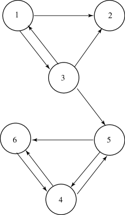
Fig. 1: A directed network with six nodes.

The adjacency matrix for this network is

$$A=\left(\begin{array}[]{cccccc}0&1&1&0&0&0\\ 0&0&0&0&0&0\\ 1&1&0&0&1&0\\ 0&0&0&0&1&1\\ 0&0&0&1&0&1\\ 0&0&0&1&0&0\\ \end{array}\right)\,.$$

The corresponding matrix $H$ is obtained by transposing $A$ and normalizing each nonzero column of $A^{T}$ by the sum of its entries:

$$H=\left(\begin{array}[]{cccccc}0&0&1/3&0&0&0\\ 1/2&0&1/3&0&0&0\\ 1/2&0&0&0&0&0\\ 0&0&0&0&1/2&1\\ 0&0&1/3&1/2&0&0\\ 0&0&0&1/2&1/2&0\\ \end{array}\right)\,.$$

Next, we modify the second column of $H$ in order to have a column-stochastic matrix:

$$S=\left(\begin{array}[]{cccccc}0&1/6&1/3&0&0&0\\ 1/2&1/6&1/3&0&0&0\\ 1/2&1/6&0&0&0&0\\ 0&1/6&0&0&1/2&1\\ 0&1/6&1/3&1/2&0&0\\ 0&1/6&0&1/2&1/2&0\\ \end{array}\right)\,.$$

Note that $S$ is reducible. Finally, we form the matrix

$$P=\alpha S+\frac{(1-\alpha)}{6}{\bf 1}{\bf 1}^{T},\quad{\rm where}\quad\alpha\in(0,1).$$

This matrix is strictly positive for any $\alpha\in(0,1)$, hence for each such $\alpha$ there is a unique dominant eigenvector, the corresponding PageRank vector.

Now we compute the PageRank vector ${\bf p}={\bf p}(\alpha)$ for different values of $\alpha$, and compare the corresponding rankings of the nodes of $G$. We begin with $\alpha=0.9$, the value used in [8, p. 39]. Rounded to five digits, the corresponding PageRank vector is

$${\bf p}(0.9)=\left(\begin{array}[]{cccccc}.03721&.05396&.04151&.37510&.20600&.28620\\ \end{array}\right)^{T}\,.$$

Therefore, the nodes of $G$ are ranked by their importance as $\left(\begin{array}[]{cccccc}4&6&5&2&3&1\end{array}\right)$.

Next we compute the PageRank vector for $\alpha=0.1$:

$${\bf p}(0.1)=\left(\begin{array}[]{cccccc}.15812&.16603&.16067&.17812&.16703&.17002\\ \end{array}\right)^{T}\,.$$

Therefore, the nodes of $G$ are ranked by their importance as $\left(\begin{array}[]{cccccc}4&6&5&2&3&1\end{array}\right)$, exactly the same ranking as before. The scores are now closer to one another (since they are all approaching the uniform probability $1/6$), but not so close as to make the ranking impossible, or different than in the case of $\alpha=0.9$.

For $\alpha=0.01$ we find

$${\bf p}(0.01)=\left(\begin{array}[]{cccccc}.16583&.16666&.16610&.16778&.16667&.16695\\ \end{array}\right)^{T}\,.$$

Again, we find that the nodes of $G$ are ranked as $\left(\begin{array}[]{cccccc}4&6&5&2&3&1\end{array}\right)$, exactly as before.

Finally, for $\alpha=0.001$ we find, rounding this time the results to seven digits:

$${\bf p}(0.001)=\left(\begin{array}[]{cccccc}.1665833&.1666666&.1666111&.1667778&.1666667&.1666945\\ \end{array}\right)^{T}\,.$$

As before, the ranking of the nodes is unchanged.

Clearly, as $\alpha$ gets smaller it becomes more difficult to rank the nodes, since the corresponding PageRank values get closer and closer together, and more accuracy is required. For this reason, it is better to avoid tiny values of $\alpha$. This is especially true for large graphs, where most of the individual entries of the PageRank vector are very small. But the important point here is that even for very small nonzero values of $\alpha$ the underlying graph structure continues to influence the rankings of the nodes. Taking values of $\alpha$ close to 1 is probably not necessary in practice, especially recalling that $\alpha$ values near 1 result in slow convergence of the PageRank iteration.

As discussed in the paper (Theorem 6.1), the rankings given by PageRank approach those obtained using the vector $H{\bf 1}$ (equivalently, $S{\bf 1}$) in the limit as $\alpha\to 0+$. This vector is given by

$$H{\bf 1}=\left(\begin{array}[]{cccccc}1/3&5/6&1/2&3/2&5/6&1\\ \end{array}\right)^{T}\,.$$

The corresponding ranking is again $\left(\begin{array}[]{cccccc}4&6&5&2&3&1\end{array}\right)$, with nodes 5 and 2 tied in third place. This is in complete agreement with our analysis. Moreover, it suggests that an inexpensive alternative to computing the PageRank vector could be simply taking the row sums of $H$. This of course amounts to ranking the nodes of the digraph using a kind of weighted in-degree. This ranking scheme is much more crude than PageRank, as we can see from the fact that it assigns the same score to nodes 2 and 5, whereas PageRank clearly gives higher importance to node 5 when $\alpha=0.9$. We make no claims about the usefulness of this ranking scheme for real directed networks, but given its low cost it may be worthy of further study.

A.2 Numerical experiments on undirected networks

In this section we present the results of numerical experiments aimed at illustrating the limiting behavior of walk-based, parameterized centrality measures using various undirected networks. We focus our attention on exponential-type and resolvent-type centrality measures, and study their relation to degree and eigenvector centrality.

The rankings produced by the various centrality measures are compared using the intersection distance method (for more information, see [6] and [1, 4]). Given two ranked lists $x$ and $y$, the top-$k$ intersection distance is computed by:

$${\rm isim}_{k}(x,y):=\frac{1}{k}\sum_{i=1}^{k}\frac{|x_{i}\Delta y_{i}|}{2i}$$

where $\Delta$ is the symmetric difference operator between the two sets and $x_{k}$ and $y_{k}$ are the top $k$ items in $x$ and $y$, respectively. The top-$k$ intersection distance gives the average of the normalized symmetric differences for the lists of the top $i$ items for all $i\leq k$. If the ordering of the top $k$ nodes is the same for the two ranking schemes, ${\rm isim}_{k}(x,y)=0$. If the top $k$ are disjoint, then ${\rm isim}_{k}(x,y)=1$. Unless otherwise specified, we compare the intersection distance for the full set of ranked nodes.

The networks come from a range of sources, although most can be found in the University of Florida Sparse Matrix Collection [5]. The first is the Zachary Karate Club network, which is a classic example in network analysis [9]. The Intravenous Drug User and the Yeast PPI networks were provided by Prof. Ernesto Estrada and are not present in the University of Florida Collection. The three Erdös networks correspond to various subnetworks of the Erdös collaboration network and can be found in the Pajek group of the UF Collection. The ca-GrQc and ca-HepTh networks are collaboration networks corresponding to the General Relativity and High Energy Physics Theory subsections of the arXiv and can be found in the SNAP group of the UF Collection. The as-735 network can also be found in the SNAP group and represents the communication network of a group of Autonomous Systems on the Internet. This communication was measured over the course of 735 days, between November 8, 1997 and January 2, 2000. The final network is the network of Minnesota roads and can be found in the Gleich group of the UF Collection. Basic data on these networks, including the order $n$, number of nonzeros, and the largest two eigenvalues, can be found in Table 3. All of the networks, with the exception of the Yeast PPI network, are simple. The Yeast PPI network has several ones on the diagonal, representing the self-interaction of certain proteins. All are undirected.

Table 3: Basic data for the networks used in the experiments.

Graph	$n$	$nnz$	$\lambda_{1}$	$\lambda_{2}$
Zachary Karate Club	34	156	6.726	4.977
Drug User	616	4024	18.010	14.234
Yeast PPI	2224	13218	19.486	16.134
Pajek/Erdos971	472	2628	16.710	10.199
Pajek/Erdos972	5488	14170	14.448	11.886
Pajek/Erdos982	5822	14750	14.819	12.005
Pajek/Erdos992	6100	15030	15.131	12.092
SNAP/ca-GrQc	5242	28980	45.617	38.122
SNAP/ca-HepTh	9877	51971	31.035	23.004
SNAP/as-735	7716	26467	46.893	27.823
Gleich/Minnesota	2642	6606	3.2324	3.2319

A.2.1 Exponential subgraph centrality and total communicability

We examined the effects of changing $\beta$ on the exponential subgraph centrality and total communicability rankings of nodes in a variety of undirected real world networks, as well as their relation to degree and eigenvector centrality. Although the only restriction on $\beta$ is that it must be greater than zero, there is often an implicit upper limit that may be problem-dependent. For the analysis in this section, we impose the following limits: $0.1\leq\beta\leq 10$. To examine the sensitivity of the exponential subgraph centrality and total communicability rankings, we calculate both sets of scores and rankings for various choices of $\beta$. The values of $\beta$ tested are: 0.1, 0.5, 1, 2, 5, 8 and 10.

The rankings produced by the matrix exponential-based centrality measures for all choices of $\beta$ were compared to those produced by degree centrality and eigenvector centrality, using the intersection distance method described above. Plots of the intersection distances for the rankings produced by various choices of $\beta$ with those produced by degree or eigenvector centrality can be found in Figs. 2 and 3. The intersection distances for rankings produced by successive choices of $\beta$ can be found in Fig. 4.

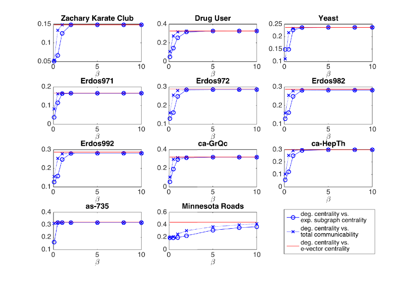
Fig. 2: The intersection distances between degree centrality and the exponential subgraph centrality (blue circles) or total communicability (blue crosses) rankings of the nodes in the networks in Table 3. The red lines are the intersection distances between degree centrality and eigenvector centrality and are added for reference.

In Figure 2, the rankings produced by exponential subgraph centrality and total communicability are compared to those produced by degree centrality. For small values of $\beta$, both sets of rankings based on the matrix exponential are very close to those produced by degree centrality (low intersection distances). When $\beta=0.1$, the largest intersection distance between the degree centrality rankings and the exponential subgraph centrality rankings for the networks examined is slightly less than 0.2 (for the Minnesota road network). The largest intersection distance between the total communicability rankings with $\beta=0.1$ and the degree centrality rankings is 0.3 (for the as-735 network). In general, the (diagonal-based) exponential subgraph centrality rankings tend to be slightly closer to the degree rankings than the (row sum-based) total communicability rankings for low values of $\beta$. As $\beta$ increases, the intersection distances increase, then level off. The rankings of nodes in networks with a very large (relative) spectral gap, such as the karate, Erdos971 and as-735 networks, stabilize extremely quickly, as expected. The one exception to the stabilization is the intersection distances between the degree centrality rankings and exponential subgraph centrality (and total communicability rankings) of nodes in the Minnesota road network. This is also expected, as the tiny ($<0.001$) spectral gap for the Minnesota road network means that it will take longer for the exponential subgraph centrality (and total communicability) rankings to stabilize as $\beta$ increases. It is worth noting that the Minnesota road network is quite different from the other ones: it is (nearly) planar, has large diameter and a much more regular degree distribution.

Fig. 3: The intersection distances between eigenvector centrality and the exponential subgraph centrality (blue circles) or total communicability (blue crosses) rankings of the nodes in the networks in Table 3. The red lines show the intersection distance between eigenvector centrality and degree centrality.

The rankings produced by exponential subgraph centrality and total communicability are compared to those produced by eigenvector centrality for various values of $\beta$ in Figure 3. When $\beta$ is small, the intersection distances are large but, as $\beta$ increases, the intersection distances quickly decrease. When $\beta=2$, they are essentially zero for all but one of the networks examined. Again, the outlier is the Minnesota road network. For this network, the intersection distances between the exponential-based centrality rankings and the eigenvector centrality rankings still decrease as $\beta$ increases, but at a much slower rate than for the other networks. This is also expected, inview of the very small spectral gap. Again, the rankings of the nodes in the karate, Erdos971, and as-735 networks, which have very large relative spectral gaps, stabilize extremely quickly.

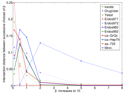
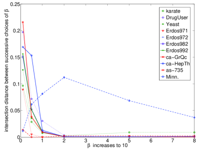
Fig. 4: The intersection distances between the exponential subgraph centrality (left) or total communicability (right) rankings produced by successive choices of $\beta$. Each line corresponds to a network in Table 3.

In Figure 4, the intersection distances between the rankings produced by exponential subgraph centrality and total communicability are compared for successive choices of $\beta$. Overall, these intersection distances are quite low (the highest is 0.25 and occurs for the exponential subgraph centrality rankings of the as-735 network when $\beta$ increases from 0.1 to 0.5). For all the networks examined, the largest intersection distances between successive choices of $\beta$ occur as $\beta$ increases to two. For higher values of $\beta$, the intersection distance drops, which corresponds to the fact that the rankings are converging to those produced by eigenvector centrality. In general, there is less change in the rankings produced by the total communicability scores for successive values of $\beta$ than for the rankings produced by the exponential subgraph centrality scores.

If the intersection distances are restricted to the top 10 nodes, they are even lower. For the karate, Erdos992, and ca-GrQc networks, the intersection distance for the top 10 nodes between successive choices of $\beta$ is always less than 0.1. For the DrugUser, Yeast, Erdos971, Erdos982, and ca-HepTh networks, the intersection distances are somewhat higher for low values of $\beta$, but by the time $\beta=2$, they are all equal to 0 as the rankings have converged to those produced by the eigenvector centrality. For the Erdos972 network, this occurs slightly more slowly. The intersection distances between the rankings of the top 10 nodes produced by $\beta=2$ and $\beta=5$ are 0.033 and for all subsequence choices of $\beta$ are 0. In the case of the Minnesota Road network, the intersection distances between the top 10 ranked nodes never stabilize to 0, as is expected. More detailed results and plots can be found in [7, Appendix B].

For the networks examined, when $\beta<0.5$, the exponential subgraph centrality and total communicability rankings are very close to those produced by degree centrality. When $\beta\geq 2$, they are essentially identical to the rankings produced by eigenvector centrality. Thus, the most additional information about node rankings (i.e. information that is not contained in the degree or eigenvector centrality rankings) is obtained when $0.5<\beta<2$. This supports the intuition developed in section 5 of the of the accompanying paper that “moderate” values of $\beta$ should be used to gain the most benefit from the use of matrix exponential-based centrality rankings.

A.2.2 Resolvent subgraph and Katz centrality

In this section we investigate the effect of changes in $\alpha$ on the resolvent subgraph centrality and Katz centrality in the networks listed in Table 3, as well as the relationship of these centrality measures to degree and eigenvector centrality. We calculate the scores and node rankings produced by degree and eigenvector centrality, as well as those produced by the resolvent ($RC_{i}(\alpha)$) and Katz ($K_{i}(\alpha)$) centralities for various values of $\alpha$. The values of $\alpha$ tested are given by $\alpha=0.01\cdot\frac{1}{\lambda_{1}}$, $0.05\cdot\frac{1}{\lambda_{1}}$, $0.1\cdot\frac{1}{\lambda_{1}}$, $0.25\cdot\frac{1}{\lambda_{1}}$, $0.5\cdot\frac{1}{\lambda_{1}}$, $0.75\cdot\frac{1}{\lambda_{1}}$, $0.9\cdot\frac{1}{\lambda_{1}}$, $0.95\cdot\frac{1}{\lambda_{1}},$ and $0.99\cdot\frac{1}{\lambda_{1}}$.

As in section A.2.1, the rankings produced by degree centrality and eigenvector centrality were compared to those produced by resolvent-based centrality measures for all choices of $\alpha$ using the intersection distance method. The results are plotted in Figs. 5 and 6. The rankings produced by successive choices of $\alpha$ are also compared and these intersection distances are plotted in Fig. 7.

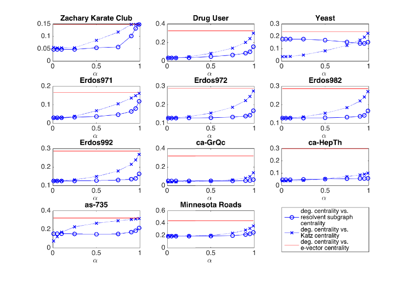
Fig. 5: The intersection distances between degree centrality and the resolvent subgraph centrality (blue circles) or Katz centrality (blue crosses) rankings of the nodes in the networks in Table 3. The $x$-axis measures $\alpha$ as a percentage of its upper bound, $\frac{1}{\lambda_{1}}$. The red lines show the intersection distances between degree centrality and eigenvector centrality for each of the networks.

Fig. 5 shows the intersection distances between the degree centrality rankings and those produced by resolvent subgraph centrality or Katz centrality for the values of $\alpha$ tested. When $\alpha$ is small, the intersection distances between the resolvent-based centrality rankings and the degree centrality rankings are low. For $\alpha=0.01\cdot\frac{1}{\lambda_{1}}$, the largest intersection distance between the degree centrality rankings and the resolvent subgraph centrality rankings is slightly less than 0.2 (for the Minnesota road network). The largest intersection distance between the degree centrality rankings and the Katz centrality rankings is also slightly less than 0.2 (again, for the Minnesota road network). The relatively large intersection distances for the node rankings on the Minnesota road network when $\alpha=0.01\cdot\frac{1}{\lambda_{1}}$ is due to the fact that with both the degree centrality and the resolvent subgraph (or Katz) centrality, there are many nodes with very close scores. Thus, small changes in the score values (induced by small changes in $\alpha$) can lead to large changes in the rankings. As $\alpha$ increases towards $\frac{1}{\lambda_{1}}$, the intersection distances increase. This increase is more rapid for the Katz centrality rankings than for the resolvent subgraph centrality rankings.

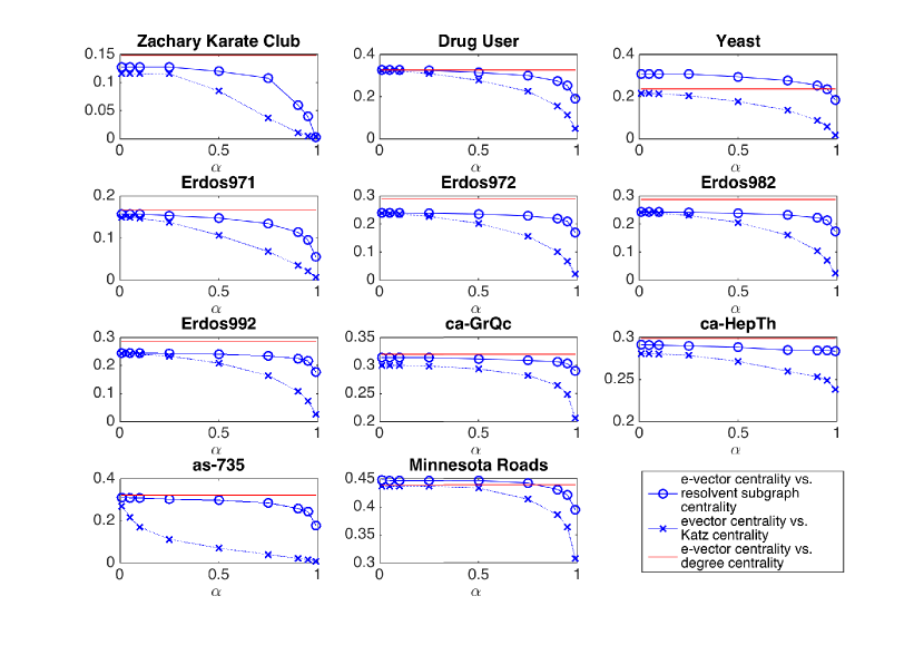
Fig. 6: The intersection distances between eigenvector centrality and the resolvent subgraph centrality (blue circles) or Katz centrality (blue crosses) rankings of the nodes in the networks in Table 3. The $x$-axis measures $\alpha$ as a percentage of its upper bound, $\frac{1}{\lambda_{1}}$. The red reference lines show the intersection distance between eigenvector centrality and degree centrality.

In Fig. 6, the resolvent subgraph centrality and Katz centrality rankings for various values of $\alpha$ are compared to the eigenvector centrality rankings on the networks described in Table 3. For small values of $\alpha$, the intersection distances tend to be large. As $\alpha$ increases, the intersection distances decrease for both resolvent subgraph centrality and Katz centrality on all of the networks examined. This decrease is faster for the (row sum-based) Katz centrality rankings than for the (diagonal-based) resolvent subgraph centrality rankings. The network with the highest intersection distances between the eigenvector centrality rankings and those based on the matrix resolvent, and slowest decrease of these intersection distances as $\alpha$ increases, is the Minnesota road network. As was the case when matrix exponential-based scores were examined, this is expected due to this network’s small spectral gap. The node rankings in networks with large relative spectral gaps (karate, Erdos971, as-735) converge to the eigenvector centrality rankings most quickly.

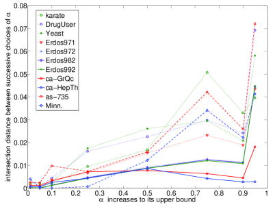
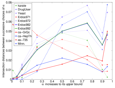
Fig. 7: The intersection distances between resolvent subgraph centrality (left) or Katz centrality (right) rankings produced by successive choices of $\alpha$. Each line corresponds to a network in Table 3.

The intersection distance between the resolvent subgraph and Katz centrality rankings produced by successive choices of $\alpha$ are plotted in Fig. 7. All of these intersection distances are extremely small (the largest is $<0.08$), indicating that the rankings do not change much as $\alpha$ increases. However, as $\alpha$ increases, the rankings corresponding to successive values of $\alpha$ tend to be slightly less similar to each other. The exception to this is the Katz centrality rankings for the as-735 network which become more similar as $\alpha$ increases.

Again, if the analysis is restricted to the top 10 nodes, the intersection distances between the rankings produced by successive choices of $\alpha$ are very small. For the karate, Erdos971, Erdos982, Erdos992, ca-GrQc, and Minnesota road networks, the intersection distances between the top 10 ranked nodes for successive choices of $\alpha$ are always less than or equal to 0.1 and often equal to zero. For the ca-HepTh network, the top 10 ranked nodes are exactly the same for all choices of $\alpha$. For the DrugUser, Yeast, and Erdos972 networks, they are always less than 0.2. Detailed results can be found in [7].

For the eleven networks examined, the resolvent subgraph and Katz centrality rankings tend to be close to the degree centrality rankings when $\alpha<0.5\cdot\frac{1}{\lambda_{1}}$. It is interesting to note that as $\alpha$ increases, these rankings stay close to the degree centrality rankings until $\alpha$ is approximately one half of its upper bound. Additionally, the resolvent based rankings are close to the eigenvector centrality rankings when $\alpha>0.9\cdot\frac{1}{\lambda_{1}}$. Thus, the most information is gained by using resolvent based centrality measures when $0.5\cdot\frac{1}{\lambda 1}\leq\alpha\leq 0.9\cdot\frac{1}{\lambda_{1}}$. This supports the intuition from section 5 of the accompanying paper that “moderate” values of $\alpha$ provide the most additional information about node ranking beyond that provided by degree and eigenvector centrality.

It is worth noting that similar conclusions have been obtained for the choice of the damping parameter $\alpha$ used in the PageRank algorithm; see [2, 3].

A.3 Numerical experiments on directed networks

In this section, we examine the relationship between the exponential and resolvent-based broadcast centrality measures with the out-degrees and the dominant right eigenvectors of two real world directed networks. A similar analysis can be done on the relationship between the receive centrality measures and the in-degrees and dominant left eigenvectors. For the experiments we use two networks from the University of Florida Sparse Matrix Collection [5]. As before, the rankings are compared using the intersection distance method. The first network we examine is wb-cs-Stanford, a network of hyperlinks between the Stanford CS webpages in 2001. It is in the Gleich group of the UF collection. The second network is the wiki-Vote network, which is a network of who votes for whom in elections for Wikipedia editors to become administrators. It is in the SNAP group of the UF collection.

Since our theory applies to strongly connected networks with irreducible adjacency matrices, our experiments were performed on the largest strongly connected component of the above networks. Basic data on these strongly connected components can be found in Table 4. In both of the networks examined, the two largest eigenvalues of the largest strongly connected component are real. Both networks are simple.

Table 4: Basic data on the largest strongly connected component of the real-world directed networks examined.

Graph	$n$	$nnz$	$\lambda_{1}$	$\lambda_{2}$
Gleich/wb-cs-Stanford	2759	13895	35.618	12.201
SNAP/wiki-Vote	1300	39456	45.145	27.573

A.3.1 Total communicability

As in section A.2.1, we examine the effect of changing $\beta$ on the broadcast total communicability rankings of nodes in the networks, as well as their relation to the rankings obtained using the out-degrees and dominant right eigenvectors of the networks. The measures were calculated for the networks described in Table 4. To examine the sensitivity of the broadcast total communicability rankings, we calculate the scores and rankings for various choices of $\beta$. The values of $\beta$ tested are: 0.1, 0.5, 1, 2, 5, 8 and 10.

The broadcast rankings produced by total communicability for all choices of $\beta$ were compared to those produced by the out-degree rankings and the rankings produced by ${\bf x}_{1}$ using the intersection distance method as described in section A.2. Plots of the intersection distances for the rankings produced by various choices of $\beta$ with those produced by the out-degrees and right dominant eigenvector can be found in Figs. 8 and 9. The intersection distances for rankings produced by successive choices of $\beta$ can be found in Figure 10.

Fig. 8: The intersection distances between the out-degree rankings and the broadcast total communicability rankings (blue circles) of the nodes in the networks in Table 4. The red reference line shows the intersection distance between the out-degree centrality and the ${\bf x}_{1}$ centrality rankings.

In Fig. 8, the intersection distances between the rankings produced by broadcast total communicability are compared to those produced by the out-degrees of nodes in the network. As $\beta$ approaches 0, the intersection distances decrease for both networks. As $\beta$ increases to 10, the intersection distances initially increase, then stabilize as the rankings converge to those produced by ${\bf x}_{1}$.

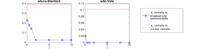
Fig. 9: The intersection distances (blue circles) between the rankings produced by ${\bf x}_{1}$ and the broadcast total communicability rankings of the nodes in the networks in Table 4. The red lines show the intersection distances between the ${\bf x}_{1}$ rankings and those produced by the out-degrees.

The intersection distances between the rankings produced by broadcast total communicability are compared to those produced by ${\bf x}_{1}$ in Figure 9. For both networks, the intersection distances quickly decrease as $\beta$ increases. In the wiki-Vote network, the intersection distances between the compared rankings are 0 by the time $\beta=0.5$. For the wb-cs-Stanford network, by the time $\beta$ has reached five, the intersection distances between the broadcast total communicability rankings and those produced by ${\bf x}_{1}$ have decreased to about 0.04. The rankings then stabilize at this intersection distance. This is due to a group of nodes that have nearly identical total communicability scores.

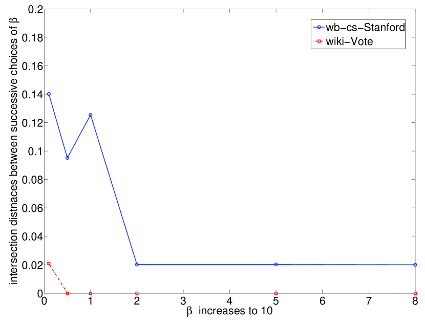
Fig. 10: The intersection distances between the broadcast total communicability rankings produced by successive choices of $\beta$. Each line corresponds to a network in Table 4.

In Fig. 10, the intersection distances between the broadcast total communicability rankings for successive choices of $\beta$ are plotted. These intersection distances are slightly lower than those observed in the undirected case, with a maximum of approximately 0.14, which occurs in the wb-cs-Stanford network when $\beta$ increases from 0.01 to 0.05. By the time $\beta=0.5$, therankings on the wiki-Vote network have stabilized and all subsequent intersection distances are 0. For both the broadcast total communicability rankings on the wb-cs-Stanford network, the intersection distances decrease (non-monotonically) as $\beta$ increases until they stabilize at approximately 0.02.

When this analysis is restricted to the top 10 nodes, the intersection distances are extremely small. For the wb-cs-Stanford network, the largest intersection distance between the top 10 ranked nodes for successive choices of $\beta$ is 0.11 (when $\beta$ increases from 0.1 to 0.5). For the wiki-Vote network, the intersection distance between the top 10 total communicability scores is 0.01 when $\beta$ increases from 0.1 to 0.5, and zero otherwise; see [7, Appendix B] for detailed results and plots.

The differences between the out-degree rankings and the broadcast total communicability rankings are greatest when $\beta\geq 0.5$. The differences between the left and right eigenvector based rankings and the broadcast rankings are greatest when $\beta<2$ (although in the case of the wiki-Vote network, they have converged by the time $\beta=0.5$). Thus, like in the case of the undirected networks, moderate values of $\beta$ give the most additional ranking information beyond that provided by the out-degrees and the left and right eigenvalues.

A.3.2 Katz centrality

In this section, we investigate the effect of changes in $\alpha$ on the broadcast Katz centrality rankings of nodes in the networks listed in Table 4 and relationship of these centrality measures to the rankings produced by the out-degrees and the dominant right eigenvectors of the network. We calculate the scores and node rankings produced by $K_{i}^{b}(\alpha)$ for various values of $\alpha$. The values of $\alpha$ tested are given by $\alpha=0.01\cdot\frac{1}{\lambda_{1}}$, $0.05\cdot\frac{1}{\lambda_{1}}$, $0.1\cdot\frac{1}{\lambda_{1}}$, $0.25\cdot\frac{1}{\lambda_{1}}$, $0.5\cdot\frac{1}{\lambda_{1}}$, $0.75\cdot\frac{1}{\lambda_{1}}$, $0.9\cdot\frac{1}{\lambda_{1}}$, $0.95\cdot\frac{1}{\lambda_{1}}$, and $0.99\cdot\frac{1}{\lambda_{1}}$.

The rankings produced by the out-degrees and the dominant right eigenvectors were compared to those produced by Katz centrality for all choices of $\alpha$ using the intersection distance method, as was done in Section A.3.1. The results are plotted in Figs. 11 and 12.

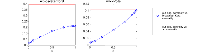
Fig. 11: The intersection distances (blue circles) between the rankings produced by the out-degrees and the broadcast Katz centrality rankings of the nodes in the networks in Table 4. Here, the $x$-axis shows $\alpha$ as a percentage of its upper bound, $\frac{1}{\lambda_{1}}$. The red reference lines show the intersection distance between the rankings produced by ${\bf x}_{1}$ and those produced by the out-degrees of the nodes.

As $\alpha$ increases from $0.01\cdot\frac{1}{\lambda_{1}}$ to $0.99\cdot\frac{1}{\lambda_{1}}$, the intersection distances between the scores produced by the broadcast Katz centralities and the out-degrees increase. When $\alpha$ is small, the broadcast Katz centrality rankings are very close to those produced by the out-degrees (low intersection distances). On the wb-cs-Stanford network, when $\alpha=0.01\cdot\frac{1}{\lambda_{1}}$, the intersection distance between the two rankings is approximately 0.06. On the wiki-Vote network, it is approximately 0.01. As $\alpha$ increases, the intersection distances also increase. By the time $\alpha=0.99\cdot\frac{1}{\lambda_{1}}$, the intersection distance between the two sets of node rankings on the wb-cs-Stanford network is above 0.2 and on the wiki-Vote network it is approximately 0.1.

Fig. 12: The intersection distances (blue circles) between the rankings produced by ${\bf x}_{1}$ and the broadcast Katz centrality rankings of the nodes in the networks in Table 4. Here, the $x$-axis shows $\alpha$ as a percentage of its upper bound, $\frac{1}{\lambda_{1}}$. The red lines show the intersection distance between the rankings produced using ${\bf x}_{1}$ and the node out-degrees.

In Fig. 12, the rankings produced by broadcast Katz centrality are compared to those produced by ${\bf x}_{1}$. Overall, The intersection distances between the two sets of rankings are lower on the wiki-Vote network than they are on the wb-cs-Stanford network. As $\alpha$ increases from $0.01\cdot\frac{1}{\lambda_{1}}$ to $0.99\cdot\frac{1}{\lambda_{1}}$, the intersection distances between the two sets of rankings on the wiki-Vote network decrease from 0.1 to essentially 0. On the wb-cs-Stanford network, they decrease from approximately 0.47 to 0.24.

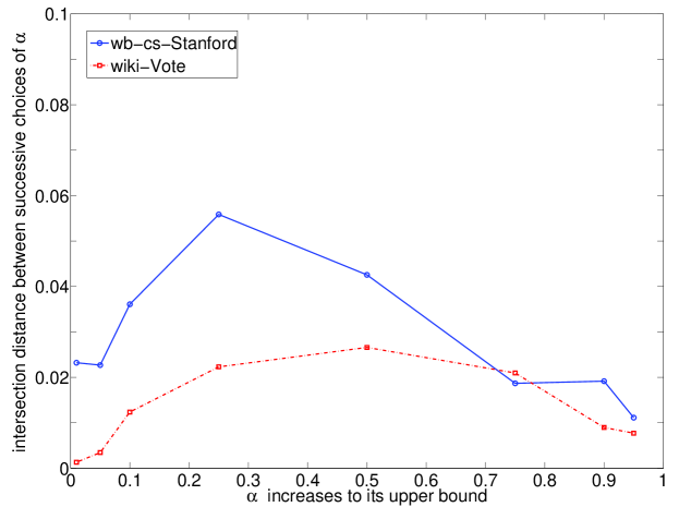
Fig. 13: The intersection distances between the broadcast Katz centrality rankings produced by successive choices of $\alpha$. Each line corresponds to a network in Table 4.

The intersection distances between the rankings produced by the broadcast Katz centralities for successive values of $\alpha$ are plotted in Figure 13. As was the case for the undirected networks, these rankings are more stable in regards to the choice of $\alpha$ than the total communicability rankings were in regards to the choice of $\beta$. Here, the maximum intersection distance is less than 0.1. When only the top 10 ranked nodes are considered, the intersection distances have a maximum of 0.06 (on the wb-cs-Stanford network when $\alpha$ increases from $0.25\cdot\frac{1}{\lambda_{1}}$ to $0.5\cdot\frac{1}{\lambda_{1}}$). For both networks, the intersection distances between the rankings on the top 10 nodes for successive choices of $\alpha$ are quite small (the maximum is 0.18 and the majority are $<0.1$).

The broadcast Katz centrality rankings are only far from those produced by the out-degrees when $\alpha\geq 0.5\cdot\frac{1}{\lambda_{1}}$. They are farthest from those produced by the dominant right eigenvector of $A$ when $\alpha<0.9\cdot\frac{1}{\lambda_{1}}$. Thus, as was seen in the case of undirected networks, the most additional information is gained when moderate values of $\alpha$, $0.5\cdot\frac{1}{\lambda_{1}}\leq\alpha<0.9\cdot\frac{1}{\lambda_{1}}$, are used to calculate the matrix resolvent based centrality scores.

Acknowledgments

Thanks to Carl Meyer for allowing us to use Fig. 1 From [8].

References

- [1] A.-L. Barabasi, Linked: The New Science of Networks, Perseus, Cambridge, UK, 2002.
- [2] A. Barrat, M. Barthelemy, and A. Vespignani, Dynamical Processes on Complex Networks, Cambridge University Press, Cambridge, UK, 2008.
- [3] M. Benzi and P. Boito, Quadrature rule-based bounds for functions of adjacency matrices, Linear Algebra Appl., 433 (2010), pp. 637–652.
- [4] M. Benzi, E. Estrada, and C. Klymko, Ranking hubs and authorities using matrix functions, Lin. Algebra Appl., 438 (2013), pp. 2447–2474.
- [5] M. Benzi and C. Klymko, Total communicability as a centrality measure, J. Complex Networks, 1(2) (2013), pp. 124–149.
- [6] S. Boccaletti, V. Latora, Y. Moreno, M. Chavez, and D.-U. Hwang, Complex networks: structure and dynamics, Phys. Rep., 424 (2006), pp. 175–308.
- [7] P. Boldi, M. Santini, and S. Vigna, PageRank as a function of the damping factor, in Proceedings of the 14th international conference on World Wide Web, Association for Computing Machinery, New York, NY (2005), pp. 557–566.
- [8] P. Boldi, M. Santini, and S. Vigna, PageRank: Functional dependencies, ACM Trans. Inf. Sys., 27(4) (2009), pp. 1–23.
- [9] P. Bonacich, Power and centrality: a family of measures, Amer. J. Sociology, 92 (1987), pp. 1170–1182.
- [10] P. Bonacich and P. Lloyd, Eigenvector-like measures of centrality for asymmetric relations, Social Networks, 23 (2001), pp. 191–201.
- [11] F. Bonchi, P. Esfandiar, D. F. Gleich, C. Greif, and L. V. S. Lakshmanan, Fast matrix computations for pair-wise and column-wise commute times and Katz scores, Internet Math., 8 (2012), pp. 73–112.
- [12] U. Brandes, On variants of shortest-path betweenness centrality and their generic computation, Social Networks, 30 (2008), pp. 136–145.
- [13] U. Brandes and T. Erlebach, eds., Network Analysis: Methodological Foundations, Lecture Notes in Computer Science Vol. 3418, Springer, New York, 2005.
- [14] S. L. Campbell and C. D. Meyer, Generalized Inverses of Linear Transformations, Dover, 1991.
- [15] T. P. Chartier, E. Kreutzer, A. N. Langville, and K. E. Pedings, Sensitivity and stability of ranking vectors, SIAM J. Sci. Comput., 33 (2011), pp. 1077–1102.
- [16] F. Chung, The heat kernel as the pagerank of a graph, Proc. Nat. Acad. Sci., 104 (2007), pp. 19735–19740.
- [17] R. Cohen and S. Havlin, Complex Networks: Structure, Robustness and Function, Cambridge University Press, Cambridge, UK, 2010.
- [18] P. Constantine and D. Gleich Random Alpha PageRank, Internet Math., 6 (2009), pp. 199–236.
- [19] D. Cvetković, P. Rowlinson, and S. Simić, Eigenspaces of Graphs, Cambridge University Press, Cambridge, UK, 1997.
- [20] R. Diestel, Graph Theory, Springer-Verlag, Berlin, 2000.
- [21] C. H. Q. Ding, H. Zha, X. He, P. Husbands, and H. D. Simon, Link analysis: hubs and authorities on the World Wide Web, SIAM Rev., 46 (2004), pp. 256–268.
- [22] S. N. Dorogovtsev and J. F. F. Mendes, Evolution of Networks: From Biological Nets to the Internet and WWW, Oxford University Press, Oxford, UK, 2003.
- [23] E. Estrada, Spectral scaling and good expansion properties in complex networks, Europhys. Lett., 73 (2006), pp. 649–655.
- [24] E. Estrada, The Structure of Complex Networks, Oxford University Press, Oxford, UK, 2011.
- [25] E. Estrada, N. Hatano, and M. Benzi, The physics of communicability in complex networks, Phys. Rep., 514 (2012), pp. 89–119.
- [26] E. Estrada and D. J. Higham, Network properties revealed through matrix functions, SIAM Rev., 52 (2010), pp. 671–696.
- [27] E. Estrada and J. A. Rodríguez-Velázquez, Subgraph centrality in complex networks, Phys. Rev. E, 71 (2005), 056103.
- [28] C. Fenu, D. Martin, L. Reichel, and G. Rodriguez, Network analysis via partial spectral factorization and Gauss quadrature, SIAM J. Sci. Comput., 35(4) (2013), pp. A2046–A2068.
- [29] C. Fenu, D. Martin, L. Reichel, and G. Rodriguez, Block Gauss and anti-Gauss quadrature with application to networks, SIAM J. Matrix Anal. Appl., 34(4) (2013), pp. 1655–1684.
- [30] L. Freeman, A set of measures of centrality based on betweenness, Sociometry, 40 (1977), pp. 35–41.
- [31] L. Freeman, Centrality in networks. I: Conceptual clarification, Social Networks, 1 (1979), 215–239.
- [32] J. R. Furlan Ronqui and G. Travieso, Analyzing complex networks through correlations in centrality measurements, arXiv:1405.7724v2 [physics.soc-ph], 2 June 2014.
- [33] R. Ghosh and K. Lerman, Parameterized centrality metric for network analysis, Phys. Rev. E, 83 (2011), 066118.
- [34] N. J. Higham, Functions of Matrices. Theory and Computation, Society for Industrial and Applied Mathematics, Philadelphia, PA, 2008.
- [35] R. A. Horn and C. R. Johnson, Matrix Analysis. Second Edition, Cambridge University Press, Cambridge, UK, 2013.
- [36] L. Katz, A new status index derived from sociometric data analysis, Psychometrika, 18 (1953), pp. 39–43.
- [37] J. Kleinberg, Authoritative sources in a hyperlinked environment, J. ACM, 46 (1999), pp. 604–632.
- [38] C. F. Klymko, Centrality and Communicability Measures in Complex Networks: Analysis and Algorithms, PhD thesis, Emory University, Atlanta, GA, 2013.
- [39] A. N. Langville and C. D. Meyer, Google’s PageRank and Beyond: The Science of Search Engine Rankings, Princeton University Press, Princeton, NJ, 2006.
- [40] A. N. Langville and C. D. Meyer, Who’s ? The Science of Rating and Ranking, Princeton University Press, Princeton, NJ, 2012.
- [41] C.-Y. Lee, Correlations among centrality measures in complex networks, arXiv:physics/0605220v1, 25 May 2006.
- [42] J. E. Marsden and I. Hoffman, Basic Complex Analysis. Fourth Edition, W. H. Freeman and Co., New York, 1987.
- [43] C. D. Meyer, Limits and the index of a square matrix, SIAM J. Appl. Math., 26 (1974), pp. 469–478.
- [44] C. D. Meyer, Matrix Analysis and Applied Linear Algebra, Society for Industrial and Applied Mathematics, Philadelphia, 2000.
- [45] M. Mihail and C. Papadimitriou, On the eigenvalue power law, in J. D. P. Rolim and S. Vadhan (Eds.), Proceedings of RANDOM 2002, Lectures Notes in Computer Science, 2483 (2002), pp. 254–262.
- [46] M. E. J. Newman, The structure and function of complex networks, SIAM Rev., 45 (2003), pp. 167–256.
- [47] M. E. J. Newman, Networks: An Introduction, Oxford University Press, Oxford, UK, 2010.
- [48] L. Page, S. Brin, R. Motwani, and T. Winograd, The PageRank Citation Ranking: Bringing Order to the Web, Tech. Report, Stanford Digital Libraries Technology Project, 1998.
- [49] J. A. Rodríguez, E. Estrada, and A. Gutíerrez, Functional centrality in graphs, Linear Multilinear Algebra, 55 (2007), pp. 293–302.
- [50] M. Romance, Local estimates for eigenvector-like centralities of complex networks, J. Comput. Appl. Math., 235 (2011), pp. 1868–1874.
- [51] M. Shimbo, T. Ito, D. Mochihashi, and Y. Matsumoto, On the properties of von Neumann kernels for link analysis, Mach. Learn., 75 (2009), pp. 37–67.
- [52] S. Vigna, Spectral ranking, arXiv:0912.0238v13, 8 November 2013.
- [53] H. Yang, I. King, and M. R. Lyu, DiffusionRank: A possible penicillin for Web spamming, SIGIR 2007 Proceedings, ACM 978-1-59593-597-7/07/0007. Association for Computing Machinery, 2007.

References

- [1] P. Boldi, TotalRank: Ranking Without Damping, in Proceedings of WWW’05, Special interest tracks and posters of the 14th international conference on World Wide Web, Association for Computing Machinery, New York, NY (2005), pp. 898–899.
- [2] P. Boldi, M. Santini, and S. Vigna, PageRank as a function of the damping factor, in Proceedings of the 14th international conference on World Wide Web, Association for Computing Machinery, New York, NY (2005), pp. 557–566.
- [3] P. Boldi, M. Santini, and S. Vigna, PageRank: Functional dependencies, ACM Trans. Inf. Sys., 27(4) (2009), pp. 1–23.
- [4] P. Constantine and D. Gleich Random Alpha PageRank, Internet Math., 6 (2009), pp. 199–236.
- [5] T. Davis and Y. Hu, The University of Florida Sparse Matrix Collection, http://www.cise.ufl.edu/research/sparse/matrices/
- [6] R. Fagin, R. Kumar, and D. Sivakumar, Comparing top lists, SIAM J. Discr. Math., 17 (2003), pp. 134–160.
- [7] C. F. Klymko, Centrality and Communicability Measures in Complex Networks: Analysis and Algorithms, PhD thesis, Emory University, Atlanta, GA, 2013.
- [8] A. N. Langville and C. D. Meyer, Google’s PageRank and Beyond: The Science of Search Engine Rankings, Princeton University Press, Princeton, NJ, 2006.
- [9] W. W. Zachary, An information flow model for conflict and fission in small groups, J. Anthrop. Res., 33 (1977), pp. 452–473.