Approximate black hole binary spacetime via asymptotic matching

Abstract

We construct a fully analytic, general relativistic, nonspinning black hole binary spacetime that approximately solves the vacuum Einstein equations everywhere in space and time for black holes sufficiently well separated. The metric is constructed by asymptotically matching perturbed Schwarzschild metrics near each black hole to a two-body post-Newtonian metric far from them, and a two-body post-Minkowskian metric farther still. Asymptotic matching is done without linearizing about a particular time slice, and thus it is valid dynamically and for all times, provided the binary is sufficiently well separated. This approximate global metric can be used for long dynamical evolutions of relativistic magnetohydrodynamical, circumbinary disks around inspiraling supermassive black holes to study a variety of phenomena.

I INTRODUCTION

The interaction between black holes and matter in the highly energetic and strong gravitational regime can reveal invaluable information both about the geometry of these dark objects, as well as the physics of magnetohydrodynamics. A particularly interesting astrophysical scenario is a circumbinary accretion disk that surrounds a supermassive black hole (SMBH) binary. As the SMBHs slowly spiral toward each other, plunge and eventually merge, the interactions between gravity and matter lead to the emission of strong electromagnetic (EM) radiation and the formation of jets. Instruments such as Pan-STARRS Kaiser et al. (2010) or the planned LSST LSST Science Collaboration et al. (2009), are designed to detect such events and characterize them up to cosmological distances (see Schnittman (2013) for a recent review on this subject).

The search and characterization of such energetic events can be aided by predicting their EM features, but such predictions require modeling. The modeling of an accretion disk about an inspiraling, SMBH binary is a challenging problem because one needs to solve the general relativistic magnetohydrodynamic (GRMHD) equations—to evolve the disk, resolve shocks, and instabilities—coupled to the full Einstein equations—to evolve the SMBH binary. In spite of the many recent breakthroughs in numerical relativity Pretorius (2005); Campanelli et al. (2006); Baker et al. (2006), a full numerical solution to the Einstein-GRMHD coupled system over many orbits is far too computationally expensive (see e.g., Farris et al. (2011); Bode et al. (2012); Giacomazzo et al. (2012)).

The modeling of circumbinary accretion disks would be greatly aided if one could calculate the SMBH binary spacetime fully analytically. The freedom to discretize the spacetime domain most appropriately for the matter evolution without also having to maintain a stable evolution of the Einstein equations leads to a more efficient and accurate simulation of the accretion disk. This is because the Courant condition greatly limits the time step size, making full numerical simulations of the spacetime impractical when the characteristic MHD speeds are significantly smaller than $c$.

The modeling of compact binaries is well suited to the post-Newtonian (PN) approximation (see e.g. Blanchet (2006)), where one solves the Einstein equations in a weak-field and a slow-motion expansion. The latter is an excellent approximation to the inspiral of compact objects, since their orbital velocity is much smaller than the speed of light until right before they plunge. The former, however, is a poor approximation to describe black holes, as their gravitational field is not weak close to the event horizon. But it is precisely this region that is of most astrophysical interest—where jets are launched, matter is swallowed up by the SMBHs, and individual accretion disks may form.

In spite of this, a PN spacetime was used in Noble et al. (2012) to study circumbinary disks, using the Harm3d code Noble et al. (2009) to solve the GRMHD equations. Because the PN approximation breaks down close to event horizons, Ref. Noble et al. (2012) was forced to excise the region encompassing the binary, precisely where one may expect very interesting EM and fluid behavior. Nonetheless, that study showed that a nontrivial and variable EM signal originated from an overdense region close to the inner edge of the disk. This lump arose after many tens of binary orbits, and therefore it had previously only been seen in Newtonian simulations Shi et al. (2012).

The main goal of this paper is to combine the PN approximation with other black hole perturbation theory ideas Yunes et al. (2006) to construct a global, purely analytical spacetime that is approximately valid everywhere in space (including close to the event horizon) and time (up until roughly $10M$, with $M$ the total mass). This metric can then be used as a background on which to solve the GRMHD equations to evolve magnetized circumbinary disks everywhere on the computational domain. In particular, it will allow the BHs to actually be on the numerical domain, making circumbinary excision unnecessary and allowing for the modeling of all relevant physics close to each event horizon. This includes the study of disk formation around individual BHs, the relativistic dynamics of gas in the interior circumbinary region and the formation of jets and shocks.

The global metric will be constructed by first subdividing the spacetime into three separate regions, where different assumptions hold and different approximations can be used. The inner zone (IZ) is the region sufficiently close to either black hole where the metric can be described by a perturbed Schwarzschild or Kerr solution Thorne (1980); Thorne and Hartle (1985); Detweiler (2005); Yunes and Gonzalez (2006); Chatziioannou et al. (2013). The near zone (NZ) is the region far away from either black hole, but less than a gravitational wave wavelength $\lambda$ from the binary’s center of mass, such that the metric can be described by a PN expansion Blanchet et al. (1998). The far or wave zone (FZ) is the region outside a gravitational wave wavelength from the binary’s center of mass, where the metric can be described by a multipolar post-Minkowskian (PM) expansion Will and Wiseman (1996). Unlike in a PN expansion, a PM treatment properly accounts for gravitational wave retardation, which is essential in the wave zone. Of course, such a subdivision of the spacetime is only valid when the SMBHs are sufficiently well separated and slowly inspiraling, breaking down at separation of roughly $10M$.

A global spacetime can then be built from the IZ, NZ and FZ metrics by asymptotically matching them inside overlapping regions of validity, or buffer zones (BZs), where adjacent metrics are simultaneously valid. The matching procedure returns a coordinate and parameter transformation relating adjacent metrics, such that the latter asymptote to each other in the BZ. Asymptotic matching in GR was carried out in Alvi (2000); Pati and Will (2000, 2002); Alvi (2003); Yunes et al. (2006); Yunes and Tichy (2006); Yunes (2007); Johnson-McDaniel et al. (2009), but always restricting attention to a particular spatial hypersurface. In this paper, we are interested in long, dynamical evolutions, and we thus lift this restriction, allowing for time-dependent, asymptotically matched transformations. Once the metrics have been asymptotically matched, a global spacetime is constructed through transition functions Yunes (2007), carefully designed to avoid introducing spurious errors in the spacetime larger than those already contained in the individual approximate metrics.

Such a global metric is an approximate solution to the vacuum Einstein equations, satisfying the latter only to the degree that the individual approximate metrics do. In order to determine the accuracy of the global metric, we compute the Ricci scalar as a function of time, as shown in Fig. 1, for two metric perturbation orders, which will be defined in Sec. II. As expected the Ricci scalar is much smaller for the second-order metric, growing with time as the inspiral proceeds and the orbital separation decreases. In this paper, we focus on nonspinning black hole binaries in a quasicircular inspiral trajectories, but the methods introduced here are valid for general black holes in generic orbits.

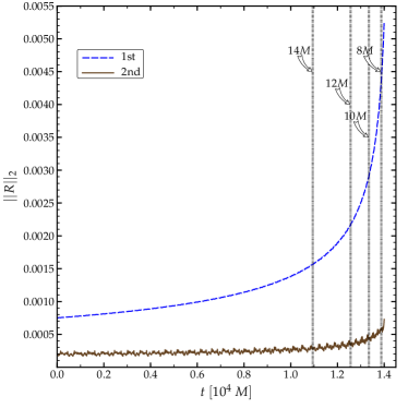
Figure 1: (Color online) L2 norm of the Ricci scalar as a function of time computed with metrics of two different perturbation orders (see Sec. II). The norms are computed using a physical domain extent of $[0,-80,-0.15]$ to $[159.95,79.95,0.1]$ in units of total mass $M$. The black hole horizons are excised and a mesh spacing of $0.05M$ is used. The black, dotted, vertical lines indicate instants of time when the binary separations reach $14M$, $12M$, $10M$ and $8M$, from left to right, respectively. The evolution is initialized at $20M$.

The remainder of this paper deals with the details of this calculation. Section II describes how to construct the global metric in more detail. Section III shows the degree to which the global metric satisfies the vacuum Einstein equations. Section IV concludes and points to future research. We mainly follow the conventions of Misner, Thorne and Wheeler Misner et al. (1973). In particular, we use greek letters $(\alpha,\beta,\cdots)$ in index lists to denote spacetime indices, and latin letters $(i,j,\cdots)$ to denote spatial indices. The metric is denoted $g_{\mu\nu}$ and it has signature $(-,+,+,+)$. We use the geometric unit system, where $G=c=1$, with the useful conversion factor $1M_{\odot}=1.477\;{\rm{km}}=4.926\times 10^{-6}\;{\rm{s}}$.

II CONSTRUCTION OF APPROXIMATE GLOBAL METRIC

In this section, we describe the construction of an approximate, global spacetime for a non-spinning binary black hole system in a quasicircular trajectory, during the inspiral regime. We begin by subdividing the spacetime into different zones, inside which different approximations will be used to obtain approximate metrics. We then explain how to connect these approximate metrics through time-dependent asymptotic matching, and conclude with a description of the transition functions necessary to glue these asymptotically matched, approximate metrics together.

II.1 Subdividing spacetime

We divide the spacetime into the following three regions:

• Inner Zone for BH1 (IZ1) and BH2 (IZ2).

• Near Zone (NZ).

• Far Zone (FZ).

Figure 2 shows a schematic representation of these three zones on a spatial hypersurface (see also Gallouin et al. (2012)). Black holes are shown as black, solid circles, with cyan circles denoting the boundaries of each zone, which are also listed in Table 1.

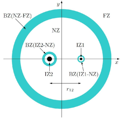
Figure 2: (Color online) Schematic diagram of the spacetime on a spatial hypersurface. BH1 and BH2 are denoted by filled, solid black circles, where the orbital separation is $r_{12}$. The BZs are denoted with cyan shells, the outer one representing the FZ-NZ BZ and the two inner ones representing the NZ-IZ BZs (see also Table 1). The circular nature of these BZs is only schematic; in practice, the BZs should be distorted. The IZ, NZ and FZ are also shown in this figure.

IZ$A$ is defined as the region sufficiently near black hole $A$ that the metric can be described as a tidally distorted black hole spacetime. Mathematically, this region can be defined via $r_{A}\ll r_{12}$, where $r_{A}$ is the distance from the $A$th black hole and $r_{12}$ is the binary’s orbital separation. The IZ metric can be modeled through black hole perturbation theory, as in Poisson (2005); Yunes and Gonzalez (2006); Detweiler (2005); Taylor and Poisson (2008); Comeau and Poisson (2009); Poisson and Vlasov (2010); Chatziioannou et al. (2013). In this paper, we concentrate on nonspinning black hole binaries, and thus, the IZ metrics will be described by a perturbed Schwarzschild solution either to quadrupole or to octupole order Poisson (2005); Detweiler (2005) in horizon-penetrating coordinates Johnson-McDaniel et al. (2009).

A highly desirable feature of the global metric for numerical purposes is the use of horizon penetrating Cook-Scheel harmonic coordinates Cook and Scheel (1997), which we will employ in the IZs. Such coordinates allow for excision of the region interior to the event horizons (especially for matter falling into the black holes). Nonpenetrating coordinates, such as standard PN harmonic coordinates, would lead to coordinate singularities and numerical difficulties on the horizons. Asymptotic matching will not spoil the horizon-penetrating properties of the global metric, since close to the horizons this metric will be that of the IZ in proper horizon-penetrating coordinates.

Table 1: Spatial regions of validity for the different zones. $r_{A}$ is the distance from the $A$th black hole with mass $m_{A}$, $r$ is the distance from the center of mass, and $r_{12}$ and $\lambda\sim\pi\sqrt{r_{12}^{3}/(m_{1}+m_{2})}$ are the orbital separation and the gravitational wavelength, respectively. For BZs to exist, the system must satisfy $m_{A}\ll r_{12}$.

Zone	Region of Validity
IZ1	$0$	$<$	$r_{1}$	$\ll$	$r_{12}$
IZ2	$0$	$<$	$r_{2}$	$\ll$	$r_{12}$
NZ	$m_{A}$	$\ll$	$r_{A}$	$\ll$	$\lambda$
FZ	$r_{12}$	$\ll$	$r$	$<$	$\infty$
IZ-NZ BZ	$m_{A}$	$\ll$	$r_{A}$	$\ll$	$r_{12}$
NZ-FZ BZ	$r_{12}$	$\ll$	$r$	$\ll$	$\lambda$

The NZ is the region sufficiently far from either black hole that the metric can be described through the PN approximation Blanchet (2006), yet is still much closer than a gravitational wavelength from the binary’s center of mass. Mathematically, this region can be defined via $m_{A}\ll r_{A}\ll\lambda$, where $m_{A}$ is the mass of the $A$th black hole and $\lambda$ is the gravitational wave wavelength. In the PN approximation, one solves the Einstein equations as an expansion in both $v/c\ll 1$ (slow motion), where $v$ is the binary’s orbital velocity and $c$ is the speed of light, and $Gm/(Rc^{2})\ll 1$ (weak fields), where $m$ is $m_{A}$ or $M=m_{A}+m_{B}$, and $R$ is $r_{A}$ or $r_{12}$. By construction, the PN approximation models black holes as point particles, expands the metric about Minkowski spacetime and models retardation in gravitational waves perturbatively. In this paper, we employ the 2.5PN NZ metric of Blanchet et al. (1998) for nonspinning black hole binaries.

The FZ is the region sufficiently far from the binary’s center of mass that the metric can be described through a multipolar, PM formalism. Mathematically, this region can be defined via $r\gg\lambda$ where $r$ is the distance from the center of mass. In this region, the metric can be obtained via direct integration of the relaxed Einstein equations Will and Wiseman (1996); Pati and Will (2000, 2002), or, alternatively, via the multipolar formalism in Blanchet et al. (1995); Blanchet (1995, 1996, 2006). Radiative effects are dominant in the FZ and retardation effects are large. In this paper, we employ a 2.5PN order PM metric, evaluated explicitly for quasicircular binaries in Johnson-McDaniel et al. (2009).

For binaries in the inspiral regime, these different zones overlap in BZs, shown as cyan shells in Fig. 2. Each IZ overlaps with the NZ, leading to 2 IZ-NZ BZs, while the NZ overlaps with the FZ in the NZ-FZ BZ. Inside the IZ-NZ BZ, the IZ’s perturbed Schwarzschild metric and the NZ’s PN metric are both simultaneously valid. Similarly, in the NZ-FZ BZ, the NZ’s PN metric and the FZ’s PM metric are simultaneously valid. The existence of such BZs is what allows one to carry out asymptotic matching and construct a global metric.

II.2 Asymptotic matching

II.2.1 Basics and prior work

Asymptotic matching is the mathematical technique that forces two approximate solutions to the same set of differential equations to asymptotically approach each other in their overlapping region of validity. This is achieved through a given coordinate and parameter transformation that relates the coordinates and parameters native to each approximation. Such transformations are obtained by setting the asymptotic expansion of the approximate solutions in the overlapping regions equal to each other.

For the problem at hand, asymptotic matching will be used to relate the perturbed Schwarzschild black hole metric of IZ$A$ to the two-body PN metric of the NZ. The NZ and FZ metrics are already asymptotically matched by construction Blanchet (2006). Through asymptotic matching, one obtains a coordinate and parameter transformation to relate IZ$A$ to the NZ, such that the transformed metric of IZ$A$ asymptotes to the NZ metric in the IZ$A$-NZ BZ.

Such a procedure to construct an approximate global metric is also ideal to compute initial data for binary black hole simulations. Alvi Alvi (2000, 2003) was the first to attempt such a construction, but ended up carrying out asymptotic patching rather than matching. Yunes et al. Yunes et al. (2006); Yunes and Tichy (2006); Yunes (2007); Johnson-McDaniel et al. (2009) succeeded in carrying out matching for nonspinning binary black holes and this data were recently evolved in Reifenberger and Tichy (2012) (see also Chu (2012) for numerical evolutions of superposed tidally perturbed BHs). Gallouin et al. Gallouin et al. (2012) recently extended this construction to spinning black hole binaries.

One may be tempted to use such a global “initial data metric” to obtain one that is valid on a large number of spatial hypersurfaces. Such a procedure, however, is doomed to fail from the start. The reason is that all initial data metrics make explicit use of expansions about $t=t_{0}$, where $t_{0}$ labels the time-parameter of the initial spatial hypersurface. Such expansions prohibits the use of the initial data metric at $t>t_{0}$, rendering them useless for dynamical evolutions. One may attempt to glue several such initial data metrics together to generate a 4-dimensional metric. However, this procedure will introduce inconsistencies in the coordinate transformations used in the matching procedure, leading to an invalid metric.

We here take a different route that is guaranteed to produce a global metric with IZ, NZ and FZ approximate metrics that asymptotically match each other for all times (up until the binary’s orbital separation becomes too small). The procedure is simply to carry out the matching without assuming $(t-t_{0})/r_{12}\ll 1$. Fortunately, part of this matching procedure has already been carried out by Taylor and Poisson Taylor and Poisson (2008). We will use the results of this paper, together with the formalism of Yunes et al. (2006); Yunes and Tichy (2006); Yunes (2007); Johnson-McDaniel et al. (2009), following closely Johnson-McDaniel et al. (2009), to construct the global metric.

We begin by reviewing the work of Taylor and Poisson Taylor and Poisson (2008). In that paper, they study the geometry of the event horizon of a nonspinning black hole that is perturbed by a companion in a quasicircular orbit. Their analysis follows Poisson’s approach to black hole perturbation theory Poisson (2004a, b, 2005); Poisson and Vlasov (2010); Comeau and Poisson (2009); Poisson et al. (2011); Chatziioannou et al. (2013), where the metric close to the black hole (the IZ metric) is expressed in ingoing Eddington-Finkelstein coordinates. This metric is composed of a background (the Schwarzschild metric) plus a metric perturbation, expressed as the product of certain functions of radius, tensor spherical harmonics of the angular coordinates, and certain functions of time. The latter characterizes the external universe (the external perturber) and it is expanded in terms of electric and magnetic tidal tensors.

Taylor and Poisson Taylor and Poisson (2008) asymptotically matched this metric to a 1PN metric in the IZ-NZ BZ. Their matching algorithm is different from the one pioneered in Yunes et al. (2006). In the latter, the matching transformation consists of both a parameter and a coordinate transformation, which is essential because the IZ and NZ metrics are not in the same coordinate system or gauge. Taylor and Poisson Taylor and Poisson (2008), instead, do a series of coordinate and gauge transformations on the IZ metric so that the end result is in harmonic coordinates and the perturbation is in harmonic gauge. Once this is done, the matching transformation just relates the parameters between the two metrics (i.e., the tidal tensors as functions of the NZ parameters).

Nowhere in the Taylor and Poisson analysis Taylor and Poisson (2008) is the IZ or NZ metrics expanded in terms of $(t-t_{0})/r_{12}\ll 1$, since they were not interested in initial data. In that paper, they in fact show by explicit calculation that asymptotic matching does not require this extra assumption, and thus, the parameter transformation they find is valid for all times, as long as a BZ exists. By composing the many coordinate transformations of Taylor and Poisson (2008), one can also obtain a time-dependent coordinate transformation that relates the IZ to the NZ metrics.

One caveat should be mentioned here before proceeding. Taylor and Poisson Taylor and Poisson (2008) only match the metric components that are needed to study the evolution of the event horizon, namely the shift and the lapse, but not the spatial metric. Moreover, they work only to 1PN order in the NZ and to quadrupole order in black hole perturbation theory in the IZ. Therefore, when applying their scheme to our problem, certain pieces of the 2PN NZ metric will not properly match to certain pieces of the octupole order IZ metric. In order for the global metric to match consistently to that order, the matching calculation would have to be redone, which will be considered elsewhere.

II.2.2 Time-dependent matching

We define the order of the matching calculation as follows. Let the IZ metric be composed of a background, such as the Schwarzschild spacetime, plus deformations of multipole orders up to $\ell=N+1$, where $N$ is an arbitrary non-negative integer. Let the NZ metric be a PN metric of $N$th PN order. With these definitions, we define the following:

• First-Order Matched Metric: Constructed from an IZ metric that consists of the Schwarzschild metric with a quadrupole deformation ($\ell=2$). This perturbation depends only on the electric quadrupole ${\cal{E}}_{ab}$ and the magnetic quadrupole ${\cal{B}}_{ab}$. The NZ metric consists of a 1PN metric.

• Second-Order Matched Metric: Constructed from an IZ metric that consists of the Schwarzschild metric with a quadrupole and an octupole deformation ($\ell=2$ and $\ell=3$). This perturbation depends on the electric quadrupole ${\cal{E}}_{ab}$ and the magnetic quadrupole ${\cal{B}}_{ab}$, as well as on their time derivatives $\dot{{\cal{E}}}_{ab}$ and $\dot{{\cal{B}}}_{ab}$, and the electric octupole ${\cal{E}}_{abc}$ and the magnetic octupole ${\cal{B}}_{abc}$. The NZ metric consists of a 2PN metric.

Of course, nothing prevents us from using the most accurate PN metric in the NZ that is available, possibly resummed in some way. However, this does not imply the IZ metric will asymptotically match the NZ metric to higher order.

The global metrics will be constructed as follows. We take the results of Johnson-McDaniel et al. (2009), which are formally valid only about a given spatial hypersurface, and perform a “temporal resummation”: we replace terms that depend on powers of $\omega t$ in the coordinate and parameter transformation of Johnson-McDaniel et al. (2009), with $\omega$ the orbital frequency, by functions of the PN orbital trajectories and velocities. For example, a term of the form $\omega t$ can be temporally resummed into $\sin{\omega t}$, which is proportional to the $y$ component of the trajectory of body 1. Similarly, a term of the form $-\omega^{2}t$ can be temporally resummed into $-\omega\sin{\omega t}$, which is proportional to the $x$ component of the velocity of body 1.

Note that the operation of temporal resummation is not unique. For example, a term of the form $\omega^{2}t^{2}$ can be temporally resummed either by $\sin^{2}{\omega t}$ or by $2(1-\cos{\omega t})$. So how does one choose the proper resummation? Here we will be guided by the work of Taylor and Poisson Taylor and Poisson (2008). We cannot use their transformations directly because they work in a different gauge and coordinate system. However, we can use the tensorial structure of their results as guiding principles to properly carry out the temporal resummation. As we will show next, using this insight, we can temporally resum the work of Johnson-McDaniel et al. (2009) to obtain an IZ metric that formally asymptotically matches the NZ metric to first order in all components and for all times. As explained in the caveat of the last subsection, we cannot use the work of Taylor and Poison to gain insight into temporal resummation at second-order in matching, since they work to first-order. Second-order, temporally resummed, asymptotic matching will have to be derived from first principles, as we will study in a future paper.

II.2.3 First-order matching

Based on Taylor and Poisson (2008), we here resum the time dependence of the coordinate transformation found in Johnson-McDaniel et al. (2009). First, we prepare various functions, as motivated by Taylor and Poisson (2008). Let us define $\tilde{x}^{i}=\{\tilde{x},\,\tilde{y},\,\tilde{z}\}$ as the coordinates centered on BH1,

$$\tilde{x} = x-{\frac{{m_{2}}\,{r_{12}}\,}{M}}\cos{\phi}\,,$$ (1)

$$\tilde{y} = y-{\frac{{m_{2}}\,{r_{12}}\,}{M}}\sin{\phi}\,,$$ (2)

$$\tilde{z} = z\,,$$ (3)

where $\tilde{r}=\sqrt{{{\tilde{x}}}^{2}+{{\tilde{y}}}^{2}+{{\tilde{z}}}^{2}}$ is the radial coordinate from BH1. The orbital phase evolution $\phi=\phi(t)$ and the evolution of the orbital separation $r_{12}=r_{12}(t)$ can be calculated in the PN formalism and must be evaluated in the same way as in the NZ PN metric. Keep in mind, however, that these quantities are both time dependent, and thus their temporal evolution must be included when computing the Jacobian of the coordinate transformation.

Let us also define the coordinates centered on BH1 that are corotating with the binary:

$$\tilde{x}_{c} = {\tilde{x}}\;\cos{\phi}\,+{\tilde{y}}\;\sin{\phi}\,,$$ (4)

$$\tilde{y}_{c} = {\tilde{y}}\;\cos{\phi}\,-{\tilde{x}}\;\sin{\phi}\,.$$ (5)

These quantities arise from the inner products $\tilde{x}^{i}\hat{x}_{(p)i}$ and $\tilde{x}^{i}\hat{v}_{(p)i}$ respectively, where $\hat{x}_{(p)i}$ and $\hat{v}_{(p)i}$ denote the unit vectors of the PN particles’ locations from the center of mass and their velocities. Note also that $\tilde{x}_{c}\sim{\tilde{x}}+\phi(t)\,{\tilde{y}}$ and $\tilde{y}_{c}\sim{\tilde{y}}-\phi(t)\,{\tilde{x}}$ for small $\phi(t)\ll 1$. If we neglect radiation-reaction, $\phi(t)=\omega t=v_{12}t/r_{12}$, so small $\phi(t)$ means an expansion in $t/r_{12}\ll 1$, precisely the expansion used in Johnson-McDaniel et al. (2009).

Let us now follow Taylor and Poisson Taylor and Poisson (2008) and introduce quantities similar to their Eqs. (7.21) and (7.22):

$$\dot{A} = \frac{1}{2}\,{\frac{{m_{2}}\,\left({m_{2}}+2\,M\right)}{M\;{r_{12}}}}\,,$$ (6)

$$R^{i} = \{0,\,0,\,R^{z}\}\,,$$ (7)

$$R^{z} = -\frac{1}{2}\,{\frac{{m_{2}}\,\left(4\,M-{m_{2}}\right)\sin{\phi}\,\cos{\phi}}{{M}\,{{r_{12}}}(1+(m_{2}-m_{2}^{2}/M-3M)/(2r_{12}))}}\,.$$ (8)

The vector $R^{i}$ shown above is obtained by simple integration, $R^{i}=\int dt\dot{R}^{i}=\dot{R}^{i}t$, where $\dot{R}^{i}$ is given in Taylor and Poisson (2008), and the last equality holds because $\dot{R}^{i}$ is constant in time, when one neglects radiation reaction. Of course, direct integration of $\dot{R}^{i}$ in Taylor and Poisson (2008) would lead to a term proportional to $\omega t$ in the spatial sector of the coordinate transformation, which is unacceptable and has here been temporally resummed. We empirically find that resumming $\omega t$ through $\sin{\phi}\cos{\phi}$ leads to proper matching at first order. Of course, the resummed form of $R^{z}$ shown above reduces exactly to the Taylor-Poisson expression for $\omega t\ll 1$. On the other hand, we temporally resum $A=\int dt\dot{A}=\int dr_{12}\dot{A}(dr_{12}/dt)^{-1}$, where the rate of change of the orbital separation $dr_{12}/dt$ is calculated from the balance law (for example, see Blanchet (2006)), because this term enters the time component of the coordinate transformation only, which evolves in the radiation reaction timescale, as we will see below. We could have resummed $R^{i}$ similarly to $A$, but we find that this is not necessary to the order we work here.

Then, taking into account the form of the coordinate transformation in Ref. Taylor and Poisson (2008), the following transformation is obtained as an extension of that in Ref. Johnson-McDaniel et al. (2009):

$$T =t-{\frac{{m_{2}}\,{\tilde{y}_{c}}}{\sqrt{{r_{12}}}\sqrt{M}}}+\frac{5}{384}\frac{(m_{2}+2M)(r_{12}^{3}-r_{12}(t_{0})^{3})}{M^{2}m_{1}}+\biggl{[}-\frac{1}{2}\,{\frac{{m_{2}}\,{\tilde{y}}\,\sqrt{M}{\tilde{x}}\,{{\tilde{r}}}^{2}}{{{r_{12}}}^{9/2}}}+\frac{1}{2}\,{\frac{{m_{2}}\,{\tilde{y}_{c}}\,\sqrt{M}{{\tilde{r}}}^{2}}{{{r_{12}}}^{7/2}}}+\frac{5}{2}\,{\frac{{m_{2}}\,{\tilde{y}}\,{{\tilde{x}}}^{3}\sqrt{M}}{{{r_{12}}}^{9/2}}}$$ (9)

$$\quad-2\,{\frac{{{\tilde{x}}}^{2}\sqrt{M}{\tilde{y}}\,{m_{2}}}{{{r_{12}}}^{7/2}}}-{\frac{{m_{2}}\,{\tilde{y}_{c}}\,{\tilde{x}_{c}}\,\left({m_{2}}-2\,M\right)}{\sqrt{M}{{r_{12}}}^{5/2}}}+\frac{1}{2}\,{\frac{{m_{2}}\,{\tilde{y}_{c}}\,\left(-5\,M+{m_{2}}\right)}{\sqrt{M}{{r_{12}}}^{3/2}}}\biggr{]}\,,$$ (10)

$$X ={\tilde{x}}+\left[-\frac{1}{2}\,{\frac{{{m_{2}}}^{2}\sin{\phi}\,{\tilde{y}_{c}}}{M{r_{12}}}}+{\tilde{x}}\,\left({\dot{A}}-\frac{1}{2}\,{\frac{{{m_{2}}}^{2}}{M{r_{12}}}}\right)+\frac{1}{2}\,{\frac{{m_{2}}\,\left(-2\,{\tilde{x}}\,{\tilde{x}_{c}}+\cos{\phi}\,{{\tilde{r}}}^{2}\right)}{{{r_{12}}}^{2}}}\right]-{\tilde{y}}\,{R^{z}}\,,$$ (11)

$$Y ={\tilde{y}}+\left[\frac{1}{2}\,{\frac{{{m_{2}}}^{2}\cos{\phi}\,{\tilde{y}_{c}}}{M{r_{12}}}}+{\tilde{y}}\,\left({\dot{A}}-\frac{1}{2}\,{\frac{{{m_{2}}}^{2}}{M{r_{12}}}}\right)+\frac{1}{2}\,{\frac{{m_{2}}\,\left(-2\,{\tilde{y}}\,{\tilde{x}_{c}}+\sin{\phi}\,{{\tilde{r}}}^{2}\right)}{{{r_{12}}}^{2}}}\right]+{\tilde{x}}\,{R^{z}}\,,$$ (12)

$$Z =z+\left[z\left({\dot{A}}-\frac{1}{2}\,{\frac{{{m_{2}}}^{2}}{M{r_{12}}}}\right)-{\frac{{m_{2}}\,z{\tilde{x}_{c}}}{{{r_{12}}}^{2}}}\right]\,,$$ (13)

The IZ1 metric components are expressed in terms of the coordinates $\{T,X,Y,Z\}$; the transformation from $\{t,x,y,z\}$ to $\{T,X,Y,Z\}$, therefore, provides a means by which we can relate points in the NZ to those in the IZ1 (with similar transformations for IZ2 after the $1\leftrightarrow 2$ exchange symmetry transformation). As mentioned earlier, notice that the temporal piece of the transformation contains the orbital separation, $r_{12}(t_{0})$, at a point in time, $t_{0}$, to describe the orbital evolution used to calculate the radiation reaction timescale; we set $t_{0}$ to be the initial time of a simulation.

Note that we have only discussed the resummation of the coordinate transformation and have not mentioned resumming the parameter transformation. The pieces of this transformation that are needed to be resummed are the relations of the multipole tidal fields as functions of the PN parameters. Such temporal resummation was already carried out in the Appendices of Johnson-McDaniel et al. (2009), and will thus not be presented again here.

With this resummed coordinate and parameter transformation, one can carry out several tests to check whether the temporal resummation was successful. First, we checked that the above transformation agrees exactly with that of Johnson-McDaniel et al. (2009) in the $\omega t\ll 1$ limit, i.e., when $t/r_{12}\ll 1$. This automatically implies that the IZ and NZ metrics matches to first order in the BZ for $t\ll r_{12}$. Second, we evaluated the transformation at a point on the horizon and plotted it as a function of time. We found that the transformation above takes this point to a trajectory identical to that of the NZ PN point particles, as expected. Third, we asymptotically expanded the transformed first-order IZ metric in the BZ and the NZ 1PN metric in the BZ (both without expanding in $t/r_{12}\ll 1$). We then compared every single metric component and found that they were identical in the BZ. This then proves that the temporally resummed transformation leads to first-order asymptotic matching for all times (as long as a BZ exists).

Before proceeding, we should mention that the transformation above is technically different from that in Taylor and Poisson (2008). In particular, we did not use the contribution to the transformation presented in their Eq. (6.16), and we changed the sign of the second term in the right-hand side of their Eq. (5.5). Their transformation and ours need not agree because Taylor and Poisson start with an IZ metric in a different gauge and coordinate system than the one used here. The functional form of the transformation, however, is indeed the same, which was crucial to select the proper temporal resummation. Ultimately, what really matters for our purposes is that the above transformation has been found to satisfy the asymptotic matching equations to first order.

II.2.4 Second-order matching

At second order in the matching, the problem becomes dramatically more complicated. Obviously, part of the complication is that the metrics in the IZ and NZ are themselves longer and more complicated (2PN versus 1PN, octupole deformation versus quadrupole). Symbolic manipulation software, such as Maple, can barely handle the necessary calculations presented here with our computational resources. But besides this, the main problem with temporally resumming the second-order matching transformation is that we have no guidance as to how to properly do it, because Taylor and Poisson only worked to first order. Without such guidance, there is an infinite number of ways in which the resummation can be carried out and not all will actually lead to a properly, second-order matched global metric.

In spite of these difficulties, we will proceed and attempt to temporally resum the transformation of Johnson-McDaniel et al. (2009) at second order in matching. First, let us take the temporally resummed transformation in Eq. (13) and expand it in $t/r_{12}\ll 1$. Comparing this to the second-order transformation in Johnson-McDaniel et al. (2009), one finds that the transformations do not agree. More in detail, the latter contains terms that do not arise upon expanding Eq. (13) in $t/r_{12}\ll 1$ and, the expanded version of Eq. (13) generated terms that are not contained in the second-order transformation of Johnson-McDaniel et al. (2009). Clearly, additional terms must be added to Eq. (13) to properly match at second order.

Let us then try to temporally resum the difference between the second-order transformation of Johnson-McDaniel et al. (2009) and the $t/r_{12}$-expanded version of Eq. (13). Using some guidance from the first-order matching calculation (but of course, as explained above, this guidance is limited), one can temporally resum the difference. The result is truly formidable, and thus, we will show it in Appendix B. Adding this resummed difference to Eq. (13) then provides a full, temporally resummed coordinate transformation to second-order in the matching. But of course, we have no guarantee that this particular choice of temporal resummation is the correct one, i.e., the one that leads to full asymptotic matching at second order for all times.

As in the first-order matching case, we can analytically investigate this last issue to see how well the second-order metric performs. First, we checked that the temporally resumed second-order transformation agrees exactly with that of Johnson-McDaniel et al. (2009) in the $\omega t\ll 1$ limit, i.e., when $t/r_{12}\ll 1$. As before, this automatically implies that the the IZ and NZ metrics match to second-order in the BZ at $t\ll r_{12}$. Second, we evaluated the transformation at a point on the horizon and plotted it as a function of time. Again, we found that the second-order transformation takes this point to a trajectory identical to that of the NZ PN point particles. Third, and perhaps most importantly, we asymptotically expanded the transformed IZ metric in the BZ and the NZ metric in the BZ (both without expanding in $t/r_{12}\ll 1$). This time, however, we did not find that all metric components matched in the BZ. That is, the temporally resummed second-order metric is not properly asymptotically matched for all times.

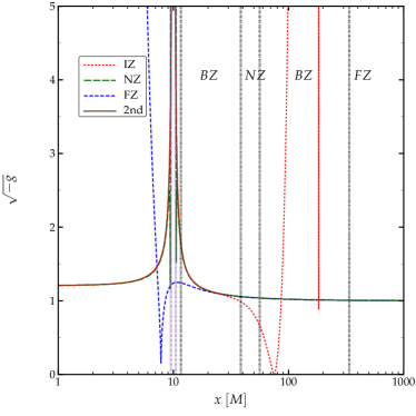
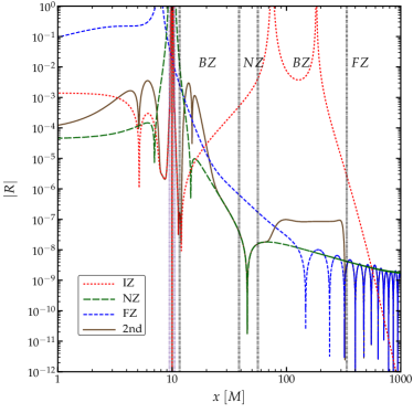
Figure 3: (Color online) Left: Comparison of the volume element, $\sqrt{-g}$, for the several different metric pieces composing the global, second-order matched metric, viz., the IZ, the NZ and the FZ metrics. Right: Absolute value of Ricci scalar computed with these metric pieces. The vertical dotted lines mark the boundaries of each zone.

For example, the off-diagonal spatial parts of the metric (e.g. $g_{12}$, $g_{13}$ and $g_{23}$) do not match at second order. At first order in the matching, one needs not worry about these components, as they simply do not enter the 1PN metric or the transformed IZ metric. Of course, at second-order in the matching, the 2PN NZ metric does have nonzero off-diagonal, spatial-spatial components, and these must be properly matched by the transformed IZ metric. In order to achieve this, we modified the resummed, second-order transformation so that many of the terms in the $(x,\,y)$ component would match. This required not only adding terms at ${\cal{O}}(v^{4})$ to the transformation, but also some at ${\cal{O}}(v^{5})$ Johnson-McDaniel et al. (2009). Given this analysis, it would seem that to complete the matching at second-order for all times, ${\cal{O}}(v^{6})$ pieces may be needed in the $t/r_{12}\ll 1$ expanded transformation, which are currently unknown. Needless to say, in spite of this improvement, the $(y,z)$ or $(x,z)$ components continue not to match at second order.

One may here wonder whether this second-order, temporally resummed matching transformation is better than the first-order one, since after all it does not properly lead to asymptotic matching in all components for all times. Evaluating the metric components, however, we empirically find that the second-order transformed IZ metric is actually much closer to the NZ metric in the BZ for all time. The improvement is roughly a factor of 5 relative to the first-order matching transformation. Of course, we suspect that if second-order, time-dependent matching were carried out properly and from first principles, the improvement between first and second-order matching would be even better (perhaps a factor of 7 or 10), but such an analysis will have to wait to future work.

II.3 Global metric

Once the IZ metrics have been transformed with the first or second-order, temporally resummed transformations, one must still glue each IZ metric to the NZ metric with proper transition functions. The global metric is then simply the weighted average

$$g_{\mu\nu} = (1-f_{\rm far})\Bigl{\{}f_{\rm near}\bigl{[}f_{{\rm inner},1}\,g_{\mu\nu}^{\rm(NZ)}+(1-f_{{\rm inner},1})\,g_{\mu\nu}^{\rm(IZ1)}\bigr{]}$$ (14)

$$+(1-f_{\rm near})\bigl{[}f_{{\rm inner},2}\,g_{\mu\nu}^{\rm(NZ)}+(1-f_{{\rm inner},2})\,g_{\mu\nu}^{\rm(IZ2)}\bigr{]}\Bigr{\}}$$

$$+f_{\rm far}\,g_{\mu\nu}^{\rm(FZ)}\,,$$

where the transition functions, $f_{\rm far}$, $f_{\rm near}$, $f_{{\rm inner},1}$ and $f_{{\rm inner},2}$ are summarized in Appendix A. The Maple scripts and C codes for the global, IZ, NZ and FZ metrics are all freely available online as “Supplemental Material” in Johnson-McDaniel et al. (2009). We have modified these scripts to include the temporally resummed matching transformation and to optimize them for speed.

Figure 3 shows how the several metric pieces contribute to the global second-order matched metric. Observe on the left panel how smoothly the IZ and NZ metric pieces approach each other in the BZ to make up the global metric. Furthermore, note on the right panel how each metric piece leads to different violations of the Ricci scalar. In particular violations outside the validity region of the several metric pieces become much larger than the ones resulting from the global metric.

III NUMERICAL ANALYSIS

Using the metric in Eq. (14), we calculate the Einstein tensor $G_{\mu\nu}$ (or Ricci tensor $R_{\mu\nu}$, Ricci scalar $R$, Hamiltonian constraint ${\cal H}$, and momentum constraint ${\cal M}_{i}$) to determine the accuracy of our approximations. Our computation does not depend on the Arnowitt-Deser-Misner (ADM, or $3+1$) decomposition Arnowitt et al. (2008), so we emphasize four dimensional quantities in our analysis below. We will here show that the Einstein tensor vanishes to the appropriate order not only at an initial moment of time, but on a sequence of time slices or arbitrary spatial extent, as expected.

III.1 Basic equations

An exact binary black hole vacuum spacetime must satisfy the ten vacuum Einstein equations $R_{\mu\nu}=0$. Hence deviations of $R=g^{\mu\nu}R_{\mu\nu}$ from zero are a measure of the error introduced in our analytical construction. We here use the conventions in Misner et al. (1973) to evaluate the Ricci scalar. Another approach to estimate the error on a given time slice is to calculate the violation of the Hamiltonian and momentum constraints. We follow here the standard conventions, for example in Nakamura et al. (1987), to compute these quantities.

Traditionally, the numerical relativity community evaluates the quality and correctness of the numerical solutions to the Einstein equations by monitoring the violation of the Hamiltonian and momentum constraints, as a function of space, time, and resolution. In analytical relativity, however, one usually computes the Einstein tensor to determine the correctness of approximate solutions. We have calculated all of these quantities and found that they present similar behavior. In this section, we present the Ricci scalar as a measure of the accuracy of the global metric.

But how should one interpret this measure? In vacuum GR, the Ricci scalar must vanish identically. The global metric constructed here, however, is approximate, and thus this scalar does not vanish identically. Physically, this error can be interpreted as a (possibly energy-condition-violating) nonvacuum component of spacetime, such as a noncollisional fluid or dust, since the Ricci scalar must be equal to the trace of the stress-energy tensor.

One would like to assess if this error is small enough to be negligible relative to other errors contained in the modeling of the system. This, of course, depends on the problem one is considering. In this paper, the problem one would eventually like to solve is the evolution of a black hole binary with a circumbinary accretion disk. It is thus natural to compare this error to the total mass present in the domain, which is dominated by the black hole masses in the IZs and the NZ. We plan on exploring further this interpretation in future work, computing the total amount of “fake” mass that would be felt by a magnetized disk as a function of the distance to the binary’s center of mass.

Before presenting a numerical analysis of the above calculations, we give rough estimates of the location of the horizon and the innermost stable circular orbit (ISCO). This will help us understand the numerical result better. For a single Schwarzschild black hole with mass $m$, the event horizon is located at $r_{\rm Hor,Sch}=2m$ and $r_{\rm Hor,Harm}=m$ in Schwarzschild and PN harmonic coordinates respectively, while the ISCO of a test particle in such a spacetime is at $r_{\rm ISCO,Sch}=6m$ and $r_{\rm ISCO,Harm}=5m$ respectively. Therefore, very roughly, the event horizon of the global metric for a binary system of comparable masses is located at $r_{A,{\rm Hor}}=0.5M$ for $A\in(1,2)$ and the ISCO is at $r_{A,{\rm ISCO}}=2.5M$ in PN harmonic coordinates, where $M=m_{1}+m_{2}$ is the total mass.

III.2 Numerical method and convergence tests

Our global approximate metric and associated analysis routines were implemented and tested both in a standalone code and in the Harm3d code. The former allowed us to perform point-wise tests of the routines anywhere on the $4$-dimensional manifold. The latter provided a platform to efficiently study the routines as a time series of $3$-dimensional slices, appropriately chosen to cover the regions around each black hole. Harm3d Noble et al. (2009, 2010, 2011) is a GRMHD code originally developed to study accretion disks around single black holes. It has recently been redesigned to handle any kind of analytic metric, including black hole binary metrics such as ours. For a review of its capabilities, please refer to Noble et al. (2012).

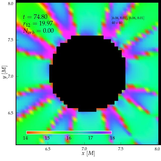
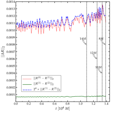
Figure 4: (Color online) Left: Convergence factor $Q^{h}$ computed using three different grid resolutions: $h=0.05M$, $h=0.025M$ and $h=0.0125M$, respectively, corresponding to $10$, $20$ and $40$ points across the horizon radius. Observe that this factor is almost everywhere close to $16$, which corresponds to fourth-order convergence. The magenta regions in this panel show areas that converge faster that fourth-order, while red regions show areas that converge slower, possibly due to zero-crossings of the solution error function. Right: L2 norm of the Ricci scalar difference for different levels of refinement as a function of time. The L2 norm is calculated over a sector of the simulation domain that ranges from $[-12,-12,-0.75]$ to $[12,12,0.75]$ with uniform resolutions following a $2:1$ Cartesian grid spacing ratio, where the coarsest grid has a mesh spacing of $0.05M$.

While the metric used in this paper is purely analytic, we chose to calculate its first and second derivatives numerically when computing the Einstein equations. We used fourth order finite difference approximations to the continuum derivative operators in a Cartesian coordinate system. Several different resolutions were employed to make sure the quantities presented are in the convergence regime to the continuum solution. We have avoided implementing an analytic version of the metric derivatives mainly due to the analytical complexity of the metric components themselves. An implementation of the analytic representation of second order mixed derivatives in time and space, for example, would not be efficient or advantageous from a computational point of view.

In our battery of tests, the first and most fundamental one is related to the convergence of the numerical solution to the analytic solution. Recall that we employed fourth-order, finite-difference approximations to the derivative operators. One way to assess the convergence rate is to look at the local convergence factor $Q^{h}(t)$ for a discrete solution function $u^{h}$ defined as

$$Q^{h}(t)=\frac{u^{4h}-u^{2h}}{u^{2h}-u^{h}}=2^{p}+O(h),$$ (15)

where $p$ is the order of the finite-difference approximation employed ($p=4$ here).

Let us now prove that our numerical implementation of Ricci scalar does indeed converge to its analytic nonzero value to fourth order, locally and globally in time. The left panel of Fig. 4 shows the convergence factor in a linear color scale ranging from $14$ to $18$. This figure shows that most of $Q^{h}$ stays in that range, suggesting fourth-order convergence. The star-ray pattern (regions where the convergence factor saturates the color scale) corresponds to regions where the discrete-solution, error function crosses zero and, therefore, cannot be appropriately represented with finite (double) machine precision. The right panel of the same figure shows the convergence of the Ricci scalar as a function of time. In particular, this figure shows the $L2$ norm of the difference of the Ricci scalar evaluated with different levels of resolution. The factor between the two curves, corresponding to the difference between medium and high levels of resolution and between low and medium ones, is close to $2^{4}$ as one can verify visually. Both panels reassure us of the correctness of our finite difference implementation.

III.3 Accuracy of global metric

We turn our attention next to how the Ricci scalar behaves as a function of the perturbative approximation order of the global metric and as a function of time. When we introduced our time resummation procedure to adapt the initial data metric to a global metric, we could have introduced artifacts or overlooked matching assumptions that could have led to undesirable errors. Figure 5 addresses these concerns by showing the Ricci scalar along the $x$ axis. The left panel shows this scalar computed with the first and the second-order metrics at a separation of $20M$. The right panel shows the scalar computed with the second-order metric at several instances of time in the evolution, starting from a separation of $20M$ and ending at $8M$. The different spacetime zones are marked with vertical lines. Observe that the magnitude of the Ricci scalar decreases as the order of the approximation increases. Furthermore, the violations increase slowly and smoothly as the orbital separation shrinks. These figures show that no artifacts or pathologies have been introduced in the global metric.

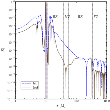
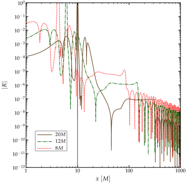
Figure 5: (Color online) Absolute value of the Ricci scalar along the $x$ axis (left) using the first and second-order metrics at a separation of $20M$ and (right) using the second-order metric at different separations. The mesh spacing is $dx=0.0125M$, roughly $40$ grid points along the horizon radius (unless indicated otherwise, the same resolution is used in all other figures). The thick purple vertical lines show the location of the event horizon, while the black ones show the boundary of the different zones. Observe how smoothly the violations to the Einstein equations increase as the orbital separation shrinks.

As a way of verifying that the second-order metric introduces fewer violations to the Einstein equations than the first-order one, we have extended our analysis to a domain consisting of a two dimensional slice, the $z=0$ plane, including one of the black holes, its IZ, NZ, and BZ. The slice is taken at a time $t=10756.60M$ (chosen because the BHs are again on the $x$ axis) when the binary separation is $r_{12}=14.13M$ after starting from $r_{12}=20M$ at $t=0M$. Figure 6 makes it clear that the trends observed above remain, i.e., that the more accurate the global metric, the closer the Ricci scalar is to zero. Thus, the smallness of the Ricci scalar computed with the second order metric is not due to plotting along the $x$ axis. In addition, this figure shows that the Ricci scalar decreases away from the black hole as expected from an approximation that asymptotically approaches Minkowski spacetime.

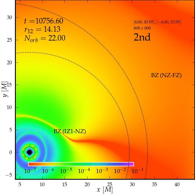
Figure 6: (Color online) Comparison of the absolute value of the Ricci scalar calculated with the first order (left) and the second order (right) metrics at $t=10756.60M$, corresponding to an orbital separation of $14.13M$, when the initial separation was $20M$. The color scale is logarithmic and fixed to emphasize the regions that saturate the interval $[10^{-7},10^{-1}]$. The concentric dotted lines centered around the black hole and the origin indicate where the IZ-NZ BZ and the NZ-FZ BZ start and end respectively.

Finally, let us include both black holes in the domain and focus our attention on the region between them and their immediate vicinity. Figure 7 shows the Ricci scalar computed with the first (left panels) and second-order metrics (right panels) at an initial separation of $20M$ (top panels) and at $t=10756.60M$ later (bottom panels), corresponding to a separation of $14.13M$. This figure shows several interesting features. First, the second order metric is globally more accurate than the first-order metric as expected. Second, the accuracy of the approximations deteriorate with shrinking orbital separation, as expected for our construction. Third, the largest violations are in the IZ-NZ BZ, just outside where the ISCO would be if the black hole were isolated. These violations correspond to the “humps” observed originally in Yunes et al. (2006) when constructing initial data. Fourth, the Ricci scalar decreases towards the perpendicular bisector of the line joining both black holes.

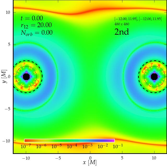
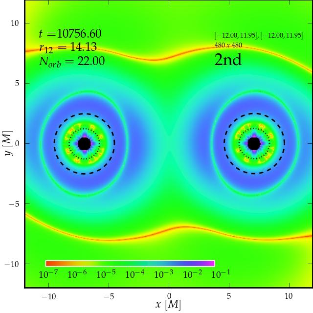
Figure 7: (Color online) Absolute value of the Ricci scalar calculated with the first-order (left) and the second-order (right) global metric at an initial separation of $20M$ (top) and after $10756.60M$ of evolution, when the separation is $14.13M$ (bottom). The color scale is logarithmic and fixed to emphasize the regions that saturates the interval $[10^{-7},10^{-1}]$. The concentric dotted and dashed lines around each black hole indicate where the IZ-NZ BZ starts and where the ISCO would be located for an individual black hole, respectively.

IV CONCLUSIONS

We have constructed a global, approximate spacetime metric that describes a nonspinning, black hole binary system in a quasicircular inspiral trajectory. This metric is built by asymptotically matching approximate metrics (a perturbed Schwarzschild metric, a two-body PN metric, and a multipolar PM metric) with a time-dependent transformation. We have evaluated the Ricci scalar as a function of time to determine how accurately this global metric satisfies the vacuum Einstein equations. We have found that indeed the metric constructed is as accurate as expected, with dominant errors arising due to uncontrolled remainders in the different approximations.

Our immediate goal is to use this metric to study a variety of astrophysical phenomena related to black hole binary spacetimes, such as the MHD evolution of accretion disks around SMBH mergers starting from astrophysically relevant initial conditions, the associated emission of electromagnetic radiation from such mergers, and the formation of jets. Upcoming work in this arena will be published in separate papers.

The specific spacetime work carried out here could be expanded in different directions. Perhaps the obvious first step is to repeat the matching calculation from first principles, without assuming $(t-t_{0})/r_{12}\ll 1$, as is done in (almost) all previous GR matching studies. Doing so to highest order possible in the matching may provide a more accurate transformation, which would thus reduce the magnitude of the uncontrolled remainders in the present metric. Another possible direction for future research would be to repeat this analysis for spinning black hole binaries. Recently, Ref. Gallouin et al. (2012) used the perturbed Kerr metric of Yunes and Gonzalez (2006) and the NZ PN metric of Faye et al. (2006) to compute an asymptotically matched metric on a short slab of spatial hypersurfaces. This asymptotically matched metric is then sufficient to construct a global metric, following the temporal-resummation prescription developed here.

Another possible avenue for future research would be to consider more generic orbits. In this paper, we focused on quasicircular, nonspinning inspirals, neglecting orbital eccentricity and precession. Recent work on eccentric inspirals Damour and Deruelle (1985); Gopakumar and Iyer (2002); Yunes et al. (2009) could be used to extend the work in Yunes et al. (2006); Yunes and Tichy (2006); Johnson-McDaniel et al. (2009); Gallouin et al. (2012) and construct an asymptotically matched spacetime for binaries in eccentric orbits.

Finally, it may be desirable to reconsider the construction of a global metric in a coordinate system that is better adapted to numerical simulations. One such set of coordinates are the ADM-TT ones, for example used in the PN work of Tichy et al. (2003); Yunes and Tichy (2006); Kelly et al. (2007, 2010); Mundim et al. (2011). One could start by constructing an asymptotically matched metric using ADM-TT coordinates in the NZ, as was done for example in Yunes and Tichy (2006). Of course, one would have to extend this work to next order in matching, which was accomplished in Johnson-McDaniel et al. (2009) using harmonic coordinates. If this is done without assuming an expansion about an initial spatial hypersurface, then the resulting global metric would be valid for all times, while a BZ exists.

Appendix A TRANSITION FUNCTIONS

When constructing a global metric, appropriate transition functions must be used to avoid introducing spurious error Yunes (2007). In this paper, we used the following piecewise function in the BZs:

$$f(r,\,r_{0},\,w,\,q,\,s)=\left\{\begin{array}[]{lr}0\,,&r\leq r_{0}\,,\\ \frac{1}{2}\left\{1+\tanh\left[\frac{s}{\pi}\left(\chi(r,\,r_{0},\,w)-\frac{q^{2}}{\chi(r,\,r_{0},\,w)}\right)\right]\right\}\,,&\hskip 25.60747ptr_{0}<r<r_{0}+w\,,\\ 1\,,&r\geq r_{0}+w\,,\end{array}\right.$$ (19)

where $\chi(r,r_{0},w)=\tan[\pi(r-r_{0})/(2w)]$, and $r_{0}$, $w$, $q$ and $s$ are parameters. References Yunes et al. (2006); Yunes and Tichy (2006); Johnson-McDaniel et al. (2009) discuss this transition function in great detail. This function satisfies the Frankenstein conditions of Yunes (2007) for an appropriate set of parameters.

The transition functions in different BZs will have slightly different parameters Johnson-McDaniel et al. (2009). We used the following throughout the paper (unless otherwise mentioned):

$$f_{\rm near} = f(x,\,2.2m_{2}-m_{1}r_{12}/M,\,r_{12}-2.2M,\,1,\,1.4)\,,$$

$$f_{{\rm inner},A} = f(r_{A},\,0.256r_{A}^{\rm T},\,3.17(M^{2}r_{12}^{5})^{1/7},\,0.2,\,r_{12}/M)\,.$$ (20)

The transition radius $r_{A}^{\rm T}=(m_{A}^{3}r_{12}^{5}/M)^{1/7}$ was derived by requiring that the uncontrolled remainders of the approximations in the IZ and NZ be comparable. The transition function in the NZ-FZ BZ was also given in Johnson-McDaniel et al. (2009) by Eq. (19) with the parameters $r_{0}=\lambda/5$, $w=\lambda$, $q=1$ and $s=2.5$, where $\lambda=\pi\sqrt{r_{12}^{3}/M}$ in the Newtonian limit. We found that this transition function leads to a rather large “bump” in the Ricci scalar $|R|$ around $x/M\approx 200$, where the transition between the NZ and FZ metrics occurs as shown in the left panel of Fig. 8.

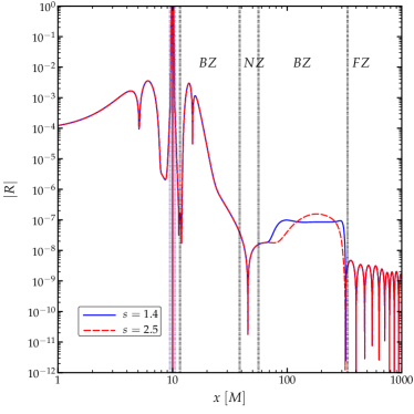
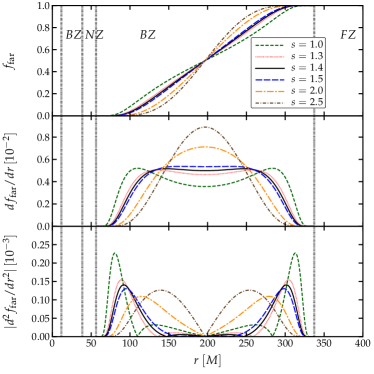
Figure 8: (Color online) Left: L2 norm of the Ricci scalar along the $x$ axis computed with the second-order metric for different choices of $s$ in the NZ-FZ BZ transition function. Observe that an appropriate choice of transition function parameter leads to a smaller “bump” in the Ricci scalar in the NZ-FZ BZ. Right: Behavior of $f_{\rm far}=f(r,\,\lambda/5,\,\lambda,\,1,\,s)$, $df_{\rm far}/dr$ and $|d^{2}f_{\rm far}/dr^{2}|$ for various values of $s$. Observe that the choice $s=1.4$ leads to a better behaved transition.

In order to remove this undesired behavior, let us study this transition function as a function of $s$ at $r_{12}/M=20$. The right panel of Fig. 8 shows $f_{\rm far}$ as well as its derivatives $df_{\rm far}/dr$ and $|d^{2}f_{\rm far}/dr^{2}|$ for various values of $s$. This figure suggests that any value of $s$ between $1.3$ and $1.5$ would lead to a better behaved NZ-FZ transition, so we here choose $s=1.4$. We have verified that with this choice of $s$, the Frankenstein theorems of Yunes (2007) are still satisfied.

Appendix B SOME DETAILS TO CONSTRUCT THE GLOBAL METRIC

In this appendix, we present in more detail the equations used to construct the global metric. In order not to duplicate equations in previous studies, let us first describe which equations we have used from previously published papers. For ease of reading, Eq. (n) from Ref. Johnson-McDaniel et al. (2009) will be denoted as Eq. (JM-n). For the NZ, the PN metric is given in Eq. (JM-4.1) (see also Eq. (7.2) of Ref. Blanchet et al. (1998) for completeness). Orbital information required to calculate the metric is taken from Ref. Blanchet (2006). For example, the phase evolution for quasicircular, nonspinning inspirals is given in Eq. (234) of Ref. Blanchet (2006). The FZ metric is obtained from Eq. (JM-6.3) with Eq. (JM-6.1), which is determined by the source multipoles in Eq. (JM-6.2). The IZ metric is given by Eq. (JM-3.2) with Eq. (JM-3.3). This metric is prescribed by multipole tidal fields in IZ coordinates $\{T,X,Y,Z\}$. The multipole tidal fields are given in Eq. (JM-B.1).

The temporally resummed coordinate transformation found in this paper (i.e., the mapping between the IZ coordinates $\{T,X,Y,Z\}$ and the PN harmonic coordinates $\{t,x,y,z\}$) to second order in the matching is explicitly

$$T =t-{\frac{{m_{2}}\,{\tilde{y}_{c}}}{\sqrt{{r_{12}}}\sqrt{M}}}+\frac{5}{384}\frac{(m_{2}+2M)(r_{12}^{3}-r_{12}(t_{0})^{3})}{M^{2}m_{1}}+\biggl{[}-\frac{1}{2}\,{\frac{{m_{2}}\,{\tilde{y}}\,\sqrt{M}{\tilde{x}}\,{{\tilde{r}}}^{2}}{{{r_{12}}}^{9/2}}}+\frac{1}{2}\,{\frac{{m_{2}}\,{\tilde{y}_{c}}\,\sqrt{M}{{\tilde{r}}}^{2}}{{{r_{12}}}^{7/2}}}+\frac{5}{2}\,{\frac{{m_{2}}\,{\tilde{y}}\,{{\tilde{x}}}^{3}\sqrt{M}}{{{r_{12}}}^{9/2}}}$$ (22)

$$\quad-2\,{\frac{{{\tilde{x}}}^{2}\sqrt{M}{\tilde{y}}\,{m_{2}}}{{{r_{12}}}^{7/2}}}-{\frac{{m_{2}}\,{\tilde{y}_{c}}\,{\tilde{x}_{c}}\,\left({m_{2}}-2\,M\right)}{\sqrt{M}{{r_{12}}}^{5/2}}}+\frac{1}{2}\,{\frac{{m_{2}}\,{\tilde{y}_{c}}\,\left(-5\,M+{m_{2}}\right)}{\sqrt{M}{{r_{12}}}^{3/2}}}\biggr{]}$$ (23)

$$\quad+\biggl{[}-4\,{\frac{\left({m_{2}}-M\right)^{2}}{{\tilde{r}}}}+2\,{\frac{{m_{2}}\,\sqrt{M}{\tilde{x}_{c}}\,\left(-2\,{{\tilde{y}_{c}}}^{2}+{{\tilde{x}_{c}}}^{2}\right)\sin{\phi}\cos{\phi}}{{r_{12}}^{7/2}}}$$ (24)

$$\qquad+{\frac{5}{1024}}\,{\frac{\left(4\,{M}^{3}-4\,{m_{2}}\,{M}^{2}-3\,{{m_{2}}}^{3}\right)(r_{12}^{2}-r_{12}(t_{0})^{2})}{{m_{1}}\,{M}^{3}}}\biggr{]}$$ (25)

$$\quad+\biggl{[}\frac{1}{12}\,{\frac{{m_{2}}\,{\tilde{y}_{c}}\,\left(6\,{{m_{2}}}^{2}+7\,{m_{2}}\,M+5\,{M}^{2}\right){{\tilde{r}}}^{2}}{\sqrt{M}{r_{12}}^{9/2}}}-\frac{14}{3}\,{\frac{{m_{2}}\,{\tilde{y}_{c}}\,\sqrt{M}{\tilde{x}_{c}}\,\left({m_{2}}-M\right){\tilde{r}}}{{r_{12}}^{9/2}}}$$ (26)

$$\qquad-{\frac{{m_{2}}\,{\tilde{y}_{c}}\,\sqrt{M}\left({m_{2}}-M\right){\tilde{r}}}{{r_{12}}^{7/2}}}+\frac{1}{4}\,{\frac{{m_{2}}\,{\tilde{y}_{c}}\,\left(M+{m_{2}}\right){{\tilde{r}}}^{2}\left(\sin{\phi}\right)^{2}\left(\cos{\phi}\right)^{2}}{\sqrt{M}{r_{12}}^{7/2}}}$$ (27)

$$\qquad-\frac{1}{3}\,{\frac{{m_{2}}\,{\tilde{y}_{c}}\,\left(6\,{{\tilde{y}_{c}}}^{2}M{m_{2}}+9\,{{\tilde{x}_{c}}}^{2}{{m_{2}}}^{2}-3\,{{\tilde{y}_{c}}}^{2}{{m_{2}}}^{2}-{{\tilde{y}_{c}}}^{2}{M}^{2}-7\,M{{\tilde{x}_{c}}}^{2}{m_{2}}+10\,{{\tilde{x}_{c}}}^{2}{M}^{2}\right)}{\sqrt{M}{r_{12}}^{9/2}}}$$ (28)

$$\qquad+\frac{1}{2}\,{\frac{{m_{2}}\,{\tilde{y}_{c}}\,{\tilde{x}_{c}}\,\left(2\,{M}^{2}+3\,{{m_{2}}}^{2}-3\,{m_{2}}\,M\right)}{\sqrt{M}{r_{12}}^{7/2}}}+\frac{1}{12}\,{\frac{{{m_{2}}}^{2}{\tilde{y}_{c}}\,\left(17\,{m_{2}}\,{M}^{2}+30\,{{m_{2}}}^{3}-17\,{{m_{2}}}^{2}M+12\,{M}^{3}\right)}{{M}^{5/2}{r_{12}}^{5/2}}}$$ (29)

$$\qquad-\frac{1}{4}\,{\frac{{m_{2}}\,{\tilde{y}_{c}}\,\left(56\,M{{\tilde{x}_{c}}}^{2}-16\,{{\tilde{y}_{c}}}^{2}M+13\,{m_{2}}\,{{\tilde{x}_{c}}}^{2}\right)\left(\sin{\phi}\right)^{2}\left(\cos{\phi}\right)^{2}}{\sqrt{M}{r_{12}}^{7/2}}}$$ (30)

$$\qquad+\frac{1}{2}\,{\frac{{m_{2}}\,{\tilde{y}_{c}}\,{\tilde{x}_{c}}\,\left(-19\,{m_{2}}\,M+3\,{{m_{2}}}^{2}+8\,{M}^{2}\right)\left(\sin{\phi}\right)^{2}\left(\cos{\phi}\right)^{2}}{{M}^{3/2}{r_{12}}^{5/2}}}+\frac{1}{24}\,{\frac{{m_{2}}\,{\tilde{y}_{c}}\,\left(\sin{\phi}\right)^{4}\left(\cos{\phi}\right)^{4}}{\sqrt{r_{12}}\sqrt{M}}}\biggr{]}\,,$$ (31)

$$X ={\tilde{x}}+\left[-\frac{1}{2}\,{\frac{{{m_{2}}}^{2}\sin{\phi}\,{\tilde{y}_{c}}}{M{r_{12}}}}+{\tilde{x}}\,\left({\dot{A}}-\frac{1}{2}\,{\frac{{{m_{2}}}^{2}}{M{r_{12}}}}\right)+\frac{1}{2}\,{\frac{{m_{2}}\,\left(-2\,{\tilde{x}}\,{\tilde{x}_{c}}+\cos{\phi}\,{{\tilde{r}}}^{2}\right)}{{{r_{12}}}^{2}}}\right]-{\tilde{y}}\,{R^{z}}$$ (32)

$$\quad+\biggl{[}-\frac{1}{8}\,{\frac{{m_{2}}\,\left(-M+2\,{m_{2}}\right){{\tilde{r}}}^{4}}{{r_{12}}^{5}}}+\frac{1}{4}\,{\frac{{m_{2}}\,\left(-{{\tilde{y}_{c}}}^{2}M-7\,M{{\tilde{x}_{c}}}^{2}+6\,{m_{2}}\,{{\tilde{x}_{c}}}^{2}\right){{\tilde{r}}}^{2}}{{r_{12}}^{5}}}-\frac{1}{2}\,{\frac{{m_{2}}\,\left({m_{2}}-M\right){{\tilde{r}}}^{3}}{{r_{12}}^{4}}}$$ (33)

$$\qquad-{\frac{{m_{2}}\,{\tilde{x}_{c}}\,\left({m_{2}}-M\right){{\tilde{r}}}^{2}}{{r_{12}}^{4}}}+3\,{\frac{{m_{2}}\,{{\tilde{x}_{c}}}^{2}\left({m_{2}}-M\right){\tilde{r}}}{{r_{12}}^{4}}}-\frac{5}{2}\,{\frac{{m_{2}}\,{{\tilde{x}_{c}}}^{4}\left({m_{2}}-M\right)}{{r_{12}}^{4}{\tilde{r}}}}+\frac{1}{2}\,{\frac{{m_{2}}\,\left(-3\,M+4\,{m_{2}}\right){{\tilde{r}}}^{2}}{{r_{12}}^{3}}}$$ (34)

$$\qquad-3\,{\frac{{m_{2}}\,{\tilde{x}_{c}}\,\left({m_{2}}-M\right){\tilde{r}}}{{r_{12}}^{3}}}+3\,{\frac{{m_{2}}\,{{\tilde{x}_{c}}}^{3}\left({m_{2}}-M\right)}{{r_{12}}^{3}{\tilde{r}}}}-2\,{\frac{\cos{\phi}{m_{2}}\,\left({m_{2}}-M\right){\tilde{r}}}{{r_{12}}^{2}}}$$ (35)

$$\qquad-\frac{1}{4}\,{\frac{{m_{2}}\,{{\tilde{x}_{c}}}^{2}\left(-7\,M{{\tilde{x}_{c}}}^{2}+5\,{m_{2}}\,{{\tilde{x}_{c}}}^{2}-11\,{{\tilde{y}_{c}}}^{2}M\right)}{{r_{12}}^{5}}}+{\frac{{m_{2}}\,{\tilde{x}_{c}}\,\left({m_{2}}\,{{\tilde{x}_{c}}}^{2}+{{\tilde{y}_{c}}}^{2}{m_{2}}-M{{\tilde{x}_{c}}}^{2}-2\,{{\tilde{y}_{c}}}^{2}M\right)}{{r_{12}}^{4}}}$$ (36)

$$\qquad+\left(-{m_{2}}\,\left(3\,{m_{2}}-2\,M\right){{\tilde{x}_{c}}}^{2}+{\frac{{m_{2}}\,\left({m_{2}}-M\right)^{2}{{\tilde{y}_{c}}}^{2}}{M}}\right)\frac{1}{r_{12}^{3}}+\frac{1}{2}\,{\frac{{m_{2}}\,\left(-7\,M+8\,{m_{2}}\right)\left({\tilde{x}_{c}}\,\cos{\phi}+{\tilde{y}_{c}}\,\sin{\phi}\right)}{{r_{12}}^{2}}}\biggr{]}$$ (37)

$$\quad+\biggl{[}-3\,{\frac{{m_{2}}\,{\tilde{y}_{c}}\,{\tilde{x}_{c}}\,\left({m_{2}}-M\right)\sin{\phi}\cos{\phi}{{\tilde{r}}}^{2}}{{r_{12}}^{5}}}-{\frac{{m_{2}}\,{\tilde{y}_{c}}\,\left({{m_{2}}}^{2}+{M}^{2}-{m_{2}}\,M\right)\sin{\phi}\cos{\phi}{{\tilde{r}}}^{2}}{M{r_{12}}^{4}}}$$ (38)

$$\qquad-6\,{\frac{{m_{2}}\,{\tilde{y}_{c}}\,{\tilde{x}_{c}}\,\left({m_{2}}-M\right)\sin{\phi}\cos{\phi}{\tilde{r}}}{{r_{12}}^{4}}}+10\,{\frac{{m_{2}}\,{{\tilde{x}_{c}}}^{3}{\tilde{y}_{c}}\,\left({m_{2}}-M\right)\sin{\phi}\cos{\phi}}{{r_{12}}^{4}{\tilde{r}}}}-3\,{\frac{{m_{2}}\,{{\tilde{x}_{c}}}^{2}{\tilde{y}_{c}}\,\left({m_{2}}-M\right)\sin{\phi}\cos{\phi}}{{r_{12}}^{3}{\tilde{r}}}}$$ (39)

$$\qquad+\frac{1}{2}\,{\frac{{m_{2}}\,{\tilde{y}_{c}}\,{\tilde{x}_{c}}\,\left(10\,{m_{2}}\,{{\tilde{x}_{c}}}^{2}-11\,{{\tilde{y}_{c}}}^{2}M-3\,M{{\tilde{x}_{c}}}^{2}\right)\sin{\phi}\cos{\phi}}{{r_{12}}^{5}}}$$ (40)

$$\qquad+\left({\frac{{m_{2}}\,\left(-{M}^{2}+3\,{{m_{2}}}^{2}+{m_{2}}\,M\right){\tilde{y}_{c}}\,{{\tilde{x}_{c}}}^{2}}{M}}-\frac{1}{2}\,{m_{2}}\,\left(-4\,M+3\,{m_{2}}\right){{\tilde{y}_{c}}}^{3}\right)\frac{\sin{\phi}\cos{\phi}}{{r_{12}}^{4}}$$ (41)

$$\qquad+{\frac{{m_{2}}\,{\tilde{y}_{c}}\,{\tilde{x}_{c}}\,\left({{m_{2}}}^{2}-4\,{m_{2}}\,M+2\,{M}^{2}\right)\sin{\phi}\cos{\phi}}{M{r_{12}}^{3}}}+\frac{1}{4}\,{\frac{{m_{2}}\,{\tilde{y}_{c}}\,\left({{m_{2}}}^{3}-5\,{{m_{2}}}^{2}M-4\,{M}^{3}-{m_{2}}\,{M}^{2}\right)\sin{\phi}\cos{\phi}}{{M}^{2}{r_{12}}^{2}}}$$ (42)

$$\qquad-\frac{1}{6}\,{\frac{{m_{2}}\,{\tilde{y}_{c}}\,{\tilde{x}_{c}}\,\left(\sin{\phi}\right)^{3}\left(\cos{\phi}\right)^{3}}{{r_{12}}^{2}}}-\frac{1}{6}\,{\frac{{m_{2}}\,{\tilde{y}_{c}}\,\left(-8\,M+5\,{m_{2}}\right)\left(\sin{\phi}\right)^{3}\left(\cos{\phi}\right)^{3}}{Mr_{12}}}\biggr{]}\,,$$ (43)

$$Y ={\tilde{y}}+\left[\frac{1}{2}\,{\frac{{{m_{2}}}^{2}\cos{\phi}\,{\tilde{y}_{c}}}{M{r_{12}}}}+{\tilde{y}}\,\left({\dot{A}}-\frac{1}{2}\,{\frac{{{m_{2}}}^{2}}{M{r_{12}}}}\right)+\frac{1}{2}\,{\frac{{m_{2}}\,\left(-2\,{\tilde{y}}\,{\tilde{x}_{c}}+\sin{\phi}\,{{\tilde{r}}}^{2}\right)}{{{r_{12}}}^{2}}}\right]+{\tilde{x}}\,{R^{z}}$$ (44)

$$\quad+\biggl{[}\frac{3}{4}\,{\frac{{\tilde{x}_{c}}\,{\tilde{y}_{c}}\,{m_{2}}\,\left(-3\,{m_{2}}+M\right){{\tilde{r}}}^{2}}{{r_{12}}^{5}}}+\frac{1}{2}\,{\frac{{\tilde{x}_{c}}\,{\tilde{y}_{c}}\,{m_{2}}\,\left({m_{2}}-M\right){\tilde{r}}}{{r_{12}}^{4}}}-\frac{5}{2}\,{\frac{{\tilde{y}}\,{m_{2}}\,{{\tilde{x}}}^{3}\left({m_{2}}-M\right)}{{r_{12}}^{4}{\tilde{r}}}}+3\,{\frac{{\tilde{y}_{c}}\,{m_{2}}\,{{\tilde{x}_{c}}}^{2}\left({m_{2}}-M\right)}{{r_{12}}^{3}{\tilde{r}}}}$$ (45)

$$\qquad-\frac{1}{4}\,{\frac{{\tilde{x}_{c}}\,{\tilde{y}_{c}}\,{m_{2}}\,\left(-21\,{m_{2}}\,{{\tilde{x}_{c}}}^{2}-6\,{{\tilde{y}_{c}}}^{2}M+13\,M{{\tilde{x}_{c}}}^{2}\right)}{{r_{12}}^{5}}}+{\frac{{\tilde{y}_{c}}\,{m_{2}}\,\left(3\,{{\tilde{x}_{c}}}^{2}-{{\tilde{y}_{c}}}^{2}\right)\left(M-{m_{2}}\right)}{{r_{12}}^{4}}}-\frac{1}{2}\,{\frac{{\tilde{x}_{c}}\,{\tilde{y}_{c}}\,{m_{2}}\,\left(2\,M-{m_{2}}\right)^{2}}{M{r_{12}}^{3}}}$$ (46)

$$\qquad+\frac{1}{8}\,{\frac{{m_{2}}\,\left({\tilde{y}_{c}}\,\cos{\phi}-{\tilde{x}_{c}}\,\sin{\phi}\right)\left(-16\,{m_{2}}\,{M}^{2}+8\,{{m_{2}}}^{2}M-{{m_{2}}}^{3}+20\,{M}^{3}\right)}{{M}^{2}{r_{12}}^{2}}}-2\,{\frac{\sin{\phi}{m_{2}}\,\left({m_{2}}-M\right){\tilde{r}}\,\cos{\phi}}{{r_{12}}^{2}}}\biggr{]}$$ (47)

$$\quad+\biggl{[}\frac{3}{4}\,{\frac{{m_{2}}\,\left({\tilde{y}_{c}}-{\tilde{x}_{c}}\right)\left({\tilde{y}_{c}}+{\tilde{x}_{c}}\right)\left(-M+3\,{m_{2}}\right)\sin{\phi}\cos{\phi}{{\tilde{r}}}^{2}}{{r_{12}}^{5}}}-\frac{3}{4}\,{\frac{{\tilde{x}_{c}}\,{{m_{2}}}^{2}\left(-M+3\,{m_{2}}\right)\sin{\phi}\cos{\phi}{{\tilde{r}}}^{2}}{M{r_{12}}^{4}}}$$ (48)

$$\qquad-\frac{1}{2}\,{\frac{{m_{2}}\,\left({\tilde{y}_{c}}-{\tilde{x}_{c}}\right)\left({\tilde{y}_{c}}+{\tilde{x}_{c}}\right)\left({m_{2}}-M\right)\sin{\phi}\cos{\phi}{\tilde{r}}}{{r_{12}}^{4}}}+\frac{1}{4}\,{\frac{{m_{2}}\,\left(4\,{m_{2}}\,M-6\,{M}^{2}+{{m_{2}}}^{2}\right)\sin{\phi}\cos{\phi}{{\tilde{r}}}^{2}}{M{r_{12}}^{3}}}$$ (49)

$$\qquad-3\,{\frac{{m_{2}}\,{\tilde{x}_{c}}\,\left({m_{2}}-M\right)\sin{\phi}\cos{\phi}{\tilde{r}}}{{r_{12}}^{3}}}+3\,{\frac{{m_{2}}\,{{\tilde{x}_{c}}}^{3}\left({m_{2}}-M\right)\sin{\phi}\cos{\phi}}{{r_{12}}^{3}{\tilde{r}}}}-8\,{\frac{{m_{2}}\,{\tilde{x}_{c}}\,\sqrt{M}\left({m_{2}}-M\right)}{{r_{12}}^{5/2}}}$$ (50)

$$\qquad-\frac{1}{4}\,{\frac{{m_{2}}\,\left(13\,{{\tilde{x}_{c}}}^{4}M-57\,M{{\tilde{x}_{c}}}^{2}{{\tilde{y}_{c}}}^{2}+63\,{m_{2}}\,{{\tilde{y}_{c}}}^{2}{{\tilde{x}_{c}}}^{2}+6\,M{{\tilde{y}_{c}}}^{4}-21\,{m_{2}}\,{{\tilde{x}_{c}}}^{4}\right)\sin{\phi}\cos{\phi}}{{r_{12}}^{5}}}$$ (51)

$$\qquad-\frac{1}{4}\,{\frac{{m_{2}}\,{\tilde{x}_{c}}\,\left(-60\,{{\tilde{y}_{c}}}^{2}M{m_{2}}+25\,M{{\tilde{x}_{c}}}^{2}{m_{2}}+36\,{{\tilde{y}_{c}}}^{2}{M}^{2}-12\,{{\tilde{x}_{c}}}^{2}{M}^{2}-21\,{{\tilde{x}_{c}}}^{2}{{m_{2}}}^{2}+18\,{{\tilde{y}_{c}}}^{2}{{m_{2}}}^{2}\right)\sin{\phi}\cos{\phi}}{M{r_{12}}^{4}}}$$ (52)

$$\qquad+\frac{1}{2}\,{\frac{{m_{2}}\,\left(-2\,M{{\tilde{x}_{c}}}^{2}{m_{2}}+2\,{{\tilde{y}_{c}}}^{2}{M}^{2}+4\,{{\tilde{x}_{c}}}^{2}{M}^{2}+2\,{{\tilde{y}_{c}}}^{2}{{m_{2}}}^{2}-{{\tilde{x}_{c}}}^{2}{{m_{2}}}^{2}-4\,{{\tilde{y}_{c}}}^{2}M{m_{2}}\right)\sin{\phi}\cos{\phi}}{M{r_{12}}^{3}}}$$ (53)

$$\qquad-\frac{1}{4}\,{\frac{{m_{2}}\,{\tilde{x}_{c}}\,\left(2\,{{m_{2}}}^{3}-4\,{M}^{3}-9\,{{m_{2}}}^{2}M-{m_{2}}\,{M}^{2}\right)\sin{\phi}\cos{\phi}}{{M}^{2}{r_{12}}^{2}}}$$ (54)

$$\qquad+\frac{1}{24}\,{\frac{{{m_{2}}}^{2}\left(-16\,{{m_{2}}}^{2}M+40\,{m_{2}}\,{M}^{2}+24\,{M}^{3}+51\,{{m_{2}}}^{3}\right)\sin{\phi}\cos{\phi}}{{M}^{3}r_{12}}}$$ (55)

$$\qquad-\frac{1}{12}\,{\frac{{m_{2}}\,\left(2\,{{m_{2}}}^{2}{r_{12}}^{2}-16\,{m_{2}}\,M{r_{12}}^{2}+16\,{M}^{2}r_{12}{\tilde{x}_{c}}-2\,{\tilde{x}_{c}}\,M{m_{2}}\,r_{12}+2\,{{\tilde{y}_{c}}}^{2}{M}^{2}-{M}^{2}{{\tilde{r}}}^{2}\right)\left(\sin{\phi}\right)^{3}\left(\cos{\phi}\right)^{3}}{{M}^{2}{r_{12}}^{2}}}$$ (56)

$$\qquad+\frac{1}{6}\,{\frac{{{m_{2}}}^{2}\left(-8\,M+{m_{2}}\right)\left(\sin{\phi}\right)^{3}\left(\cos{\phi}\right)^{3}}{{M}^{2}}}+{\frac{1}{120}}\,{\frac{{m_{2}}\,\left(\sin{\phi}\right)^{5}\left(\cos{\phi}\right)^{5}r_{12}}{M}}\biggr{]}\,,$$ (57)

$$Z =z+\left[z\left({\dot{A}}-\frac{1}{2}\,{\frac{{{m_{2}}}^{2}}{M{r_{12}}}}\right)-{\frac{{m_{2}}\,z{\tilde{x}_{c}}}{{{r_{12}}}^{2}}}\right]$$ (58)

$$\quad+\biggl{[}\frac{1}{4}\,{\frac{{m_{2}}\,z{\tilde{x}_{c}}\,\left(-9\,{m_{2}}+M\right){{\tilde{r}}}^{2}}{{r_{12}}^{5}}}+\frac{1}{2}\,{\frac{z{{m_{2}}}^{2}{{\tilde{r}}}^{2}}{{r_{12}}^{4}}}-\frac{1}{2}\,{\frac{{m_{2}}\,z{\tilde{x}_{c}}\,\left(M-{m_{2}}\right){\tilde{r}}}{{r_{12}}^{4}}}+\frac{5}{2}\,{\frac{{m_{2}}\,z{{\tilde{x}_{c}}}^{3}\left(M-{m_{2}}\right)}{{r_{12}}^{4}{\tilde{r}}}}$$ (59)

$$\qquad-3\,{\frac{{m_{2}}\,z{{\tilde{x}_{c}}}^{2}\left(M-{m_{2}}\right)}{{r_{12}}^{3}{\tilde{r}}}}-\frac{3}{4}\,{\frac{{m_{2}}\,z{\tilde{x}_{c}}\,\left(-7\,{m_{2}}\,{{\tilde{x}_{c}}}^{2}-2\,{{\tilde{y}_{c}}}^{2}M+M{{\tilde{x}_{c}}}^{2}\right)}{{r_{12}}^{5}}}$$ (60)

$$\qquad+{\frac{{m_{2}}\,z\left({{\tilde{y}_{c}}}^{2}{m_{2}}-{{\tilde{y}_{c}}}^{2}M-3\,{m_{2}}\,{{\tilde{x}_{c}}}^{2}+M{{\tilde{x}_{c}}}^{2}\right)}{{r_{12}}^{4}}}+\frac{1}{2}\,{\frac{{m_{2}}\,z\left(M-{m_{2}}\right)}{{r_{12}}^{2}}}\biggr{]}$$ (61)

$$\quad+\biggl{[}\frac{1}{4}\,{\frac{{\tilde{y}_{c}}\,{m_{2}}\,z\left(9\,{m_{2}}-M\right)\sin{\phi}\cos{\phi}{{\tilde{r}}}^{2}}{{r_{12}}^{5}}}-\frac{1}{2}\,{\frac{{\tilde{y}_{c}}\,{m_{2}}\,z\left({m_{2}}-M\right)\sin{\phi}\cos{\phi}{\tilde{r}}}{{r_{12}}^{4}}}$$ (62)

$$\qquad+\frac{15}{2}\,{\frac{{\tilde{y}_{c}}\,{m_{2}}\,{{\tilde{x}_{c}}}^{2}z\left({m_{2}}-M\right)\sin{\phi}\cos{\phi}}{{r_{12}}^{4}{\tilde{r}}}}-\frac{3}{4}\,{\frac{{\tilde{y}_{c}}\,{m_{2}}\,z\left(-7\,M{{\tilde{x}_{c}}}^{2}+2\,{{\tilde{y}_{c}}}^{2}M+21\,{m_{2}}\,{{\tilde{x}_{c}}}^{2}\right)\sin{\phi}\cos{\phi}}{{r_{12}}^{5}}}$$ (63)

$$\qquad-\frac{1}{2}\,{\frac{{\tilde{x}_{c}}\,{\tilde{y}_{c}}\,{m_{2}}\,z\left(8\,{M}^{2}-23\,{m_{2}}\,M+9\,{{m_{2}}}^{2}\right)\sin{\phi}\cos{\phi}}{M{r_{12}}^{4}}}-\frac{1}{6}\,{\frac{{\tilde{y}_{c}}\,{m_{2}}\,z\left(\sin{\phi}\right)^{3}\left(\cos{\phi}\right)^{3}}{{r_{12}}^{2}}}\biggr{]}\,.$$ (64)

The second-order transformed IZ metric under the PN harmonic coordinates is calculated by using the above equations.

References

- Kaiser et al. (2010) N. Kaiser, W. Burgett, K. Chambers, L. Denneau, J. Heasley, R. Jedicke, E. Magnier, J. Morgan, P. Onaka, and J. Tonry, in Society of Photo-Optical Instrumentation Engineers (SPIE) Conference Series, Society of Photo-Optical Instrumentation Engineers (SPIE) Conference Series, Vol. 7733 (2010).
- LSST Science Collaboration et al. (2009) LSST Science Collaboration, P. A. Abell, J. Allison, S. F. Anderson, J. R. Andrew, J. R. P. Angel, L. Armus, D. Arnett, S. J. Asztalos, T. S. Axelrod, and et al., ArXiv e-prints (2009), arXiv:0912.0201 [astro-ph.IM] .
- Schnittman (2013) J. D. Schnittman, Class. Quantum Grav. 30, 244007 (2013), arXiv:1307.3542 [gr-qc] .
- Pretorius (2005) F. Pretorius, Phys. Rev. Lett. 95, 121101 (2005), arXiv:gr-qc/0507014 .
- Campanelli et al. (2006) M. Campanelli, C. O. Lousto, P. Marronetti, and Y. Zlochower, Phys. Rev. Lett. 96, 111101 (2006), gr-qc/0511048 .
- Baker et al. (2006) J. G. Baker, J. Centrella, D.-I. Choi, M. Koppitz, and J. van Meter, Phys. Rev. Lett. 96, 111102 (2006), gr-qc/0511103 .
- Farris et al. (2011) B. D. Farris, Y. T. Liu, and S. L. Shapiro, Phys. Rev. D84, 024024 (2011), arXiv:1105.2821 [astro-ph.HE] .
- Bode et al. (2012) T. Bode, T. Bogdanović, R. Haas, J. Healy, P. Laguna, and D. Shoemaker, Astrophys. J. 744, 45 (2012), arXiv:1101.4684 [gr-qc] .
- Giacomazzo et al. (2012) B. Giacomazzo, J. G. Baker, M. C. Miller, C. S. Reynolds, and J. R. van Meter, Astrophys. J. 752, L15 (2012), arXiv:1203.6108 [astro-ph.HE] .
- Blanchet (2006) L. Blanchet, Living Rev. Relativity 9, 4 (2006).
- Noble et al. (2012) S. C. Noble, B. C. Mundim, H. Nakano, J. H. Krolik, M. Campanelli, et al., Astrophys. J. 755, 51 (2012), arXiv:1204.1073 [astro-ph.HE] .
- Noble et al. (2009) S. C. Noble, J. H. Krolik, and J. F. Hawley, Astrophys. J. 692, 411 (2009), arXiv:0808.3140 .
- Shi et al. (2012) J.-M. Shi, J. H. Krolik, S. H. Lubow, and J. F. Hawley, Astrophys. J. 749, 118 (2012), arXiv:1110.4866 [astro-ph.HE] .
- Yunes et al. (2006) N. Yunes, W. Tichy, B. J. Owen, and B. Bruegmann, Phys. Rev. D74, 104011 (2006), arXiv:gr-qc/0503011 .
- Thorne (1980) K. S. Thorne, Rev. Mod. Phys. 52, 299 (1980).
- Thorne and Hartle (1985) K. S. Thorne and J. B. Hartle, Phys. Rev. D31, 1815 (1985).
- Detweiler (2005) S. L. Detweiler, Class. Quantum Grav. 22, S681 (2005), arXiv:gr-qc/0501004 .
- Yunes and Gonzalez (2006) N. Yunes and J. A. Gonzalez, Phys. Rev. D73, 024010 (2006), arXiv:gr-qc/0510076 .
- Chatziioannou et al. (2013) K. Chatziioannou, E. Poisson, and N. Yunes, Phys. Rev. D87, 044022 (2013), arXiv:1211.1686 [gr-qc] .
- Blanchet et al. (1998) L. Blanchet, G. Faye, and B. Ponsot, Phys. Rev. D58, 124002 (1998), arXiv:gr-qc/9804079 .
- Will and Wiseman (1996) C. M. Will and A. G. Wiseman, Phys. Rev. D54, 4813 (1996), arXiv:gr-qc/9608012 .
- Alvi (2000) K. Alvi, Phys. Rev. D61, 124013 (2000), arXiv:gr-qc/9912113 .
- Pati and Will (2000) M. E. Pati and C. M. Will, Phys. Rev. D62, 124015 (2000), arXiv:gr-qc/0007087 .
- Pati and Will (2002) M. E. Pati and C. M. Will, Phys. Rev. D65, 104008 (2002), arXiv:gr-qc/0201001 .
- Alvi (2003) K. Alvi, Phys. Rev. D67, 104006 (2003), arXiv:gr-qc/0302061 .
- Yunes and Tichy (2006) N. Yunes and W. Tichy, Phys. Rev. D74, 064013 (2006), arXiv:gr-qc/0601046 .
- Yunes (2007) N. Yunes, Class. Quantum Grav. 24, 4313 (2007), arXiv:gr-qc/0611128 .
- Johnson-McDaniel et al. (2009) N. K. Johnson-McDaniel, N. Yunes, W. Tichy, and B. J. Owen, Phys. Rev. D80, 124039 (2009), arXiv:0907.0891 [gr-qc] .
- Misner et al. (1973) C. W. Misner, K. Thorne, and J. A. Wheeler, Gravitation (W. H. Freeman & Co., San Francisco, 1973).
- Gallouin et al. (2012) L. Gallouin, H. Nakano, N. Yunes, and M. Campanelli, Class. Quantum Grav. 29, 235013 (2012), arXiv:1208.6489 [gr-qc] .
- Poisson (2005) E. Poisson, Phys. Rev. Lett. 94, 161103 (2005), arXiv:gr-qc/0501032 .
- Taylor and Poisson (2008) S. Taylor and E. Poisson, Phys. Rev. D78, 084016 (2008), arXiv:0806.3052 [gr-qc] .
- Comeau and Poisson (2009) S. Comeau and E. Poisson, Phys. Rev. D80, 087501 (2009), arXiv:0908.4518 [gr-qc] .
- Poisson and Vlasov (2010) E. Poisson and I. Vlasov, Phys. Rev. D81, 024029 (2010), arXiv:0910.4311 [gr-qc] .
- Cook and Scheel (1997) G. B. Cook and M. A. Scheel, Phys. Rev. D56, 4775 (1997).
- Blanchet et al. (1995) L. Blanchet, T. Damour, and B. R. Iyer, Phys. Rev. D51, 5360 (1995), arXiv:gr-qc/9501029 .
- Blanchet (1995) L. Blanchet, Phys. Rev. D51, 2559 (1995), arXiv:gr-qc/9501030 .
- Blanchet (1996) L. Blanchet, Phys. Rev. D54, 1417 (1996), arXiv:gr-qc/9603048 .
- Bender and Orszag (1999) C. M. Bender and S. A. Orszag, Advanced mathematical methods for scientists and engineers 1, Asymptotic methods and perturbation theory (Springer, New York, 1999).
- Reifenberger and Tichy (2012) G. Reifenberger and W. Tichy, Phys. Rev. D86, 064003 (2012), arXiv:1205.5502 [gr-qc] .
- Chu (2012) T. Chu, Numerical simulations of black-hole spacetimes, Ph.D. thesis, California Institute of Technology, Pasadena, CA 91125, USA (2012).
- Poisson (2004a) E. Poisson, Phys. Rev. D69, 084007 (2004a), arXiv:gr-qc/0311026 .
- Poisson (2004b) E. Poisson, Phys. Rev. D70, 084044 (2004b), arXiv:gr-qc/0407050 .
- Poisson et al. (2011) E. Poisson, A. Pound, and I. Vega, Living Rev. Relativity 14, 7 (2011), arXiv:1102.0529 [gr-qc] .
- Arnowitt et al. (2008) R. L. Arnowitt, S. Deser, and C. W. Misner, Gen. Rel. Grav. 40, 1997 (2008), arXiv:gr-qc/0405109 .
- Nakamura et al. (1987) T. Nakamura, K. Oohara, and Y. Kojima, Prog. Theor. Phys. Suppl. 90, 1 (1987).
- Noble et al. (2010) S. C. Noble, J. H. Krolik, and J. F. Hawley, Astrophys. J. 711, 959 (2010), arXiv:1001.4809 [astro-ph.HE] .
- Noble et al. (2011) S. C. Noble, J. H. Krolik, J. D. Schnittman, and J. F. Hawley, Astrophys. J. 743, 115 (2011), arXiv:1105.2825 [astro-ph.HE] .
- Faye et al. (2006) G. Faye, L. Blanchet, and A. Buonanno, Phys. Rev. D74, 104033 (2006), arXiv:gr-qc/0605139 .
- Damour and Deruelle (1985) T. Damour and N. Deruelle, Ann. Inst. Henri Poincaré Phys. Théor., 43, 107 (1985).
- Gopakumar and Iyer (2002) A. Gopakumar and B. R. Iyer, Phys. Rev. D65, 084011 (2002), arXiv:gr-qc/0110100 .
- Yunes et al. (2009) N. Yunes, K. Arun, E. Berti, and C. M. Will, Phys. Rev. D80, 084001 (2009), arXiv:0906.0313 [gr-qc] .
- Tichy et al. (2003) W. Tichy, B. Bruegmann, M. Campanelli, and P. Diener, Phys. Rev. D67, 064008 (2003), arXiv:gr-qc/0207011 .
- Kelly et al. (2007) B. J. Kelly, W. Tichy, M. Campanelli, and B. F. Whiting, Phys. Rev. D76, 024008 (2007), arXiv:0704.0628 [gr-qc] .
- Kelly et al. (2010) B. J. Kelly, W. Tichy, Y. Zlochower, M. Campanelli, and B. F. Whiting, Class. Quantum Grav. 27, 114005 (2010), arXiv:0912.5311 [gr-qc] .
- Mundim et al. (2011) B. C. Mundim, B. J. Kelly, Y. Zlochower, H. Nakano, and M. Campanelli, Class. Quantum Grav. 28, 134003 (2011), arXiv:1012.0886 [gr-qc] .