Energy-Based Atomistic-to-Continuum
Coupling Without Ghost Forces

Abstract.

We present a practical implementation of an energy-based atomistic-to-continuum (a/c) coupling scheme without ghost forces, and numerical tests evaluating its accuracy relative to other types of a/c coupling schemes.

1. Introduction

Atomistic-to-continuum coupling methods (a/c methods) are a class of computational multiscale schemes that combine the accuracy of atomistic models of defects with the computational efficiency of continuum models of elastic far-fields [6, 15, 24, 23]. In the present article, we present the first succesful implementation of a practical patch test consistent energy based a/c coupling scheme. Previously such schemes were only available for 2-body interactions [20, 21]

In recent years a numerical analysis theory of a/c methods has emerged; we refer to [11] for a review. This theory has identified three prototypical classes of a/c schemes: patch test consistent energy-based coupling, force-based coupling (including force-based blending), and energy-based blending. The classical numerical analysis concepts of consistency and stability are applied to precisely quantify the errors committed in these schemes, and clear guidelines are established for their practical implementation including optimisation of approximation parameters. The results in [2, 14, 11, 16, 19] indicate that patch test consistent a/c couplings observe (quasi-)optimal error estimates in the energy-norm. However, to this date, no general construction and implementation of such schemes has been presented. Instead, one normally compromises by either turning to patch test consistent force-based schemes [22, 9, 8, 6] or to blending schemes [24, 12] which have some control over the consistency error. Quasi-optimal implementations of such schemes are described in [12, 8].

Existing patch test consistent schemes are restricted in their range of validity: [23] is only consistent for flat a/c interfaces and short-ranged interactions, [4] extends the idea to arbitrary range and [19] to domains with corners (but restricting again to nearest-neighbour interaction). On the other hand, the schemes presented in [20, 21, 13] are valid for general interaction range and a/c interfaces with corners, but are restricted to pair interactions.

In the present article, we shall present a generalisation of the geometric reconstruction technique [23, 4, 19], which we subsequently denote GRAC. Briefly, the idea is that, instead of evaluating the interatomic potential near the a/c interface with atom positions obtained by interpolating the continuum description, one extrapolates atom positions from those in the atomistic region (geometric reconstruction). This idea is somewhat analogous to the implementation of Neumann boundary conditions for finite difference schemes. There is substantial freedom in how this reconstruction is achieved, leading to a number of free parameters. One then determines these reconstruction parameters by solving the “geometric consistency equations” [4], which encode a form of patch test consistency and lead to a first-order consistent coupling scheme [16].

The works [4, 19, 16] have demonstrated that GRAC is a promising approach, but also indicate that explicit analytical determination of the reconstruction parameters for general a/c interface geometries with general interaction range may be impractical. Instead we propose to compute the reconstruction parameters in a preprocessing step. Although this is a natural idea it has not been pursued to the best of our knowledge.

A number of challenges must be overcome to obtain a robust numerical scheme in this way. The two key issues we will discuss are:

• If the geometric consistency equations have a solution then it is not unique. The consistency analysis [16] suggests that a solution is best selected through $\ell^{1}$-minimisation of the coefficients. Indeed, we shall demonstrate that the least squares solution leads to prohibitively large errors.

• In [17] we proved that there exists no universally stable a/c coupling of geometric reconstruction type. We will see that this is in fact of practical concern and demonstrate that the stabilisation mechanism proposed in [17] appears to resolve this issue.

In the remainder of the paper we present a complete description of a practical implementation of the GRAC method (§ 2) and numerical experiments focused primarily on investigating approximation errors (§ 3). We will comment on open issues and possible improvements in § 4, which are primarily concerned with the computational cost of determining the reconstruction coefficients.

2. Formulation of the GRAC Method

In formulating the GRAC scheme, we adopt the point of view of [5], where the computational domain and boundary conditions are considered part of the approximation. This setting is convenient to assess approximation errors. Adaptions of the coupling mechanism to other problems are straightforward.

We first present a brief review, ignoring some technical details, of a model for crystal defects in an infinite lattice from [5], and some results concerning their structure (§ 2.1). In § 2.2 we present a generic form of a/c coupling schemes, which we then specialize to the GRAC scheme in § 2.3. In § 2.3 and in § 2.4 we address, respectively, the two key issues (A) and (B) mentioned in the introduction.

For the sake of simplicity of presentation, and to emphasize the algorithmic aspects of the GRAC method, we restrict the presentation to relatively simple settings such as point defects and microcracks as in [12, 8]. The concepts required to generalize the presentation to problems involving dislocations can be found in [5].

2.1. Atomistic model

Let $d\in\{2,3\}$ denote the problem dimension. Fix a non-singular ${\sf A}\in\mathbb{R}^{d\times d}$ to define a Bravais lattice ${\sf A}\mathbb{Z}^{d}$. Let $\Lambda\subset\mathbb{R}^{d}$ be a discrete reference configuration of a crystal, possibly with a local defect: for some compact domain $\Omega^{\rm def}$ we assume that $\Lambda\setminus\Omega^{\rm def}={\sf A}\mathbb{Z}^{d}\setminus\Omega^{\rm def}$ and $\Lambda\cap\Omega^{\rm def}$ is finite. It can be readily seen [5], that certain point defects (e.g., interstials, vacancies; see Figure 1) can be enforced that way.

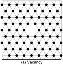
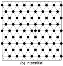
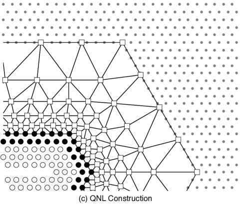
Figure 1. (a, b) Examples of reference configurations $\Lambda$ with point defects embedded. (c) Construction of the QNL method: $\circ$ atomistic potential $\Phi_{\ell}$; $\bullet$ interface potential $\Phi_{\ell}^{\rm i}$; $\square$ Cauchy–Born potential $W$ (precisely, $W$ is applied on elements/triangles); $\bullet$ far-field boundary condition $y(\ell)={\sf B}\ell$ is imposed.

To avoid minor technical difficulties, we prescribe a maximal interaction neighbourhood in the reference configuration. This is a restriction that can be lifted with little additional work [5, Remark 2.1]. For each $\ell\in\Lambda$ we denote this neighbourhood by $\mathscr{N}(\ell):=\{\ell^{\prime}\in\Lambda\,|\,|\ell^{\prime}-\ell|\leq r_{\rm cut}\}$, for some specified reference cut-off radius $r_{\rm cut}$. We define the assocated sets $\mathscr{N}_{*}(\ell):=\mathscr{N}(\ell)\setminus\{\ell\}$ and $\mathscr{R}(\ell):=\{\ell^{\prime}-\ell\,|\,\ell^{\prime}\in\mathscr{N}_{*}(\ell)\}$. We define the “finite difference stencil” $Dv(\ell):=(D_{\rho}v(\ell))_{\rho\in\mathscr{R}(\ell)}:=(v(\ell+\rho)-v(\ell))_{\rho\in\mathscr{R}(\ell)}$. Higher-order finite differences, $D_{\rho}D_{\varsigma}v$ and $D^{2}v$ are defined in a canonical way.

We use this notation to define a discrete energy space. For $v:\Lambda\to\mathbb{R}^{m}$, let the discrete energy-norm be defined by

$$\|v\|_{\dot{\mathscr{W}}^{1,2}}:=\|Dv\|_{\ell^{2}}:=\bigg{(}\sum_{\ell\in\Lambda}\sum_{\rho\in\mathscr{R}(\ell)}\frac{|D_{\rho}v(\ell)|^{2}}{|\rho|^{2}}\bigg{)}^{1/2}=\bigg{(}\sum_{\ell\in\Lambda}\sum_{\ell^{\prime}\in\mathscr{N}_{*}(\ell)}\frac{|v(\ell^{\prime})-v(\ell)|^{2}}{|\ell^{\prime}-\ell|^{2}}\bigg{)}^{1/2},$$

which we can think of as a discrete $H^{1}$-seminorm. Then, the associated discrete function space is defined by

$$\dot{\mathscr{W}}^{1,2} :=\big{\{}u:\Lambda\to\mathbb{R}^{m}\,\big{|}\,\|u\|_{\dot{\mathscr{W}}^{1,2}}<+\infty\big{\}}.$$

The space $\dot{\mathscr{W}}^{1,2}$ can be thought of as the space of all relative displacements with finite energy.

For a deformed configuration $y:\Lambda\to\mathbb{R}^{d}$ and $\ell\in\Lambda$, let $\Phi_{\ell}(y)=\Phi_{\ell}((y_{\ell^{\prime}})_{\ell^{\prime}\in\mathscr{N}(\ell)})$ denote a site energy functional associated with $\ell$. For $\ell\in\Lambda\setminus\Omega^{\rm def}$ we assume that $\Phi_{\ell}(y)\equiv\Phi(y-y(\ell))$, i.e., the crystal is homogeneous outside $\Omega^{\rm def}$. By changing the interaction potential inside $\Omega^{\rm def}$, impurities or “cut bonds” can be modelled.

The prototypical example is the embedded atom model [1], for which $\Phi_{\ell}$ is of the form

$$\begin{split}\Phi_{\ell}(y)&=\sum_{\ell^{\prime}\in\mathscr{N}_{*}(\ell)}\phi\big{(}|y(\ell^{\prime})-y(\ell)|\big{)}+F\Big{(}{\textstyle\sum_{\ell^{\prime}\in\mathscr{N}_{*}(\ell)}}\psi\big{(}|y(\ell^{\prime})-y(\ell)|\big{)}\Big{)}\\ &=\sum_{\rho\in\mathscr{R}(\ell)}\phi\big{(}|D_{\rho}y(\ell)|\big{)}+F\Big{(}{\textstyle\sum_{\rho\in\mathscr{R}(\ell)}}\psi\big{(}|D_{\rho}y(\ell)|\big{)}\Big{)}.\end{split}$$ (2.1)

The energy of an infinite configuration is typically ill-defined, but the energy-difference functional

$$E(y;z)=\sum_{\ell\in\Lambda}\Phi_{\ell}(y)-\Phi_{\ell}(z)$$

is a meaningful object. For example, if $y-z$ has compact support, then $E(y;z)$ is well-defined. More generally it is shown in [5, Thm. 2.2], under natural technical conditions on the site potentials $\Phi_{\ell}$, that $u\mapsto E(y^{\sf B}+u;y^{\sf B}),u\in\dot{\mathscr{W}}^{1,2}$, is well-defined and (Fréchet) differentiable, where $y^{\sf B}(x)={\sf B}x$.

Given a macroscopic applied strain ${\sf B}\in\mathbb{R}^{d\times d}$, we aim to compute

$$y\in\arg\min\big{\{}E(y;y^{\sf B})\,\big{|}\,y-y^{\sf B}\in\dot{\mathscr{W}}^{1,2}\big{\}}.$$ (2.2)

A solution to (2.2) will satisfy the far-field boundary condition $y(\ell)\sim{\sf B}\ell$ as $|\ell|\to\infty$, imposed through the condition that $y-y^{\sf B}\in\dot{\mathscr{W}}^{1,2}$.

We call a solution $y$ strongly stable if there exists $c_{0}>0$ such that $\langle\delta^{2}E(y)v,v\rangle\geq c_{0}\|Dv\|_{\ell^{2}}^{2}$ for all $v\in\dot{\mathscr{W}}^{1,2}$.

Here, and throughout, we write $\delta^{j}E(y)$ instead of $\delta^{j}E(y;z)$ since the variations of the energy difference only depend on the first component.

Remark 2.1. The far-field boundary condition $y(\ell)\sim{\sf B}\ell$ can be generalised to any deformation $y_{0}$ satisfying $\delta E(y_{0})\in(\dot{\mathscr{W}}^{1,2})^{*}$, for example, to dislocations by replacing ${\sf B}\ell$ with the linear elasticity solution of the dislocation [5]. ∎

2.2. A/C coupling

We begin by giving a generic formulation of an a/c coupling, which we subsequently make concrete employing concepts and notation from various earlier works, such as [15, 22, 23, 12], but adapting the formulation to our setting of § 2. The construction is visualised in Figure 1(c).

To choose a computational domain let $\Omega\subset\mathbb{R}^{d}$ be a simply connected, polygonal and closed set. We decompose $\Omega=\Omega^{\rm a}\cup\Omega^{\rm c}$, where $\Omega^{\rm a}$ is again simply connected and polygonal, and contains the defect: $\Omega^{\rm def}\subset\Omega^{\rm a}$. Let $\mathscr{T}_{h}$ be a regular partition of $\Omega^{\rm c}$ into triangles ($d=2$) or tetrahedra ($d=3$). Let $I_{h}$ denote the associated nodal interpolation operator.

Next, we decompose the set $\Lambda^{{\rm a},{\rm i}}:=\Lambda\cap\Omega^{\rm a}=\Lambda^{\rm a}\cup\Lambda^{\rm i}$ into a core atomistic region $\Lambda^{\rm a}$ and an interface region $\Lambda^{\rm i}$ (typically a few “layers” of atoms surrounding $\Lambda^{\rm a}$).

We can now define the space of coarse-grained displacement maps,

$$\mathscr{W}_{h}:=\big{\{}u_{h}:\Omega^{\rm c}\cup\Lambda^{{\rm a},{\rm i}}\to\mathbb{R}^{m}\,\big{|}\,~{} u_{h} \mathscr{T}_{h}$$ is continuous and p.w. affine w.r.t. ,

$$\text{ and $u_{h}=0$ on $\partial\Omega$ }\big{\}}.$$

The associated space of coarse-grained deformations is $y^{\sf B}+\mathscr{W}_{h}$.

The Cauchy–Born strain energy function is given by

$$W({\sf F}):=|{\rm vor}(\ell)|^{-1}\Phi_{\ell}({\sf F}\cdot\mathscr{R}(\ell))\qquad\text{ for some }\ell\in\Lambda\setminus\Omega^{\rm def},$$

where ${\rm vor}(\ell)$ is the voronoi cell associated with $\ell$. (Due to the homogeneity of the lattice and interaction outside $\Omega^{\rm def}$, the definition is independent of $\ell$.)

For $\ell\in\Lambda^{{\rm i}}$, we choose a modified interface site potential $\Phi_{\ell}^{\rm i}$ and an effective cell $v_{\ell}^{\rm i}\subset{\rm vor}(\ell)$ associated with $\ell$ (specific choices will be specified in § 2.3), and define the effective volume associated with $\ell$ as $\omega^{{\rm i}}_{\ell}:=|v_{\ell}^{\rm i}|/|{\rm vor}(\ell)|$. Further, for each element $T\in\mathscr{T}_{h}$ we define the effective volume $\omega_{T}:=|T\setminus(\cup_{\ell\in\Lambda^{{\rm i}}}v^{\rm i}_{\ell})|$.

Then, a generic a/c coupling energy difference functional is then defined by

$$E^{\rm ac}(y_{h};z_{h}) :=\sum_{\ell\in\Lambda^{\rm a}}\Big{(}\Phi_{\ell}(y_{h})-\Phi_{\ell}(z_{h})\Big{)}+\sum_{\ell\in\Lambda^{\rm i}}\omega^{\rm i}_{\ell}\Big{(}\Phi^{\rm i}_{\ell}(y_{h})-\Phi_{\ell}^{\rm i}(z_{h})\Big{)}$$ (2.3)

$$\qquad+\sum_{T\in\mathscr{T}_{h}}\omega_{T}\Big{(}W(\nabla y_{h}|_{T})-W(\nabla z_{h}|_{T})\Big{)}.$$

Thus, we obtain the approximate variational problem

$$y_{h}\in\arg\min\big{\{}E^{\rm ac}(y_{h};y^{\sf B})\,\big{|}\,y_{h}-y^{\sf B}\in\mathscr{W}_{h}\big{\}}.$$ (2.4)

2.2.1. The patch tests

A key condition that has been widely discussed in the a/c coupling literature is that $E^{\rm ac}$ should exhibit no “ghost forces”. Following the language of [16], we call this condition the force patch test: for $\Lambda={\sf A}\mathbb{Z}^{d}$ and $\Phi_{\ell}\equiv\Phi$ (homogeneous lattice without defects)

$$\langle\delta E^{\rm ac}(y^{\sf F}),v\rangle=0\qquad\forall v\in\mathscr{W}_{h},\quad{\sf F}\in\mathbb{R}^{d\times d}.$$ (2.5)

In addition, to guarantee that $E^{\rm ac}$ approximates the atomistic energy $E$, it is reasonable to also require that the interface potentials satisfy an energy patch test

$$\Phi_{\ell}^{\rm i}(y^{\sf F})=\Phi_{\ell}(y^{\sf F})\qquad\forall{\sf F}\in\mathbb{R}^{d\times d},\quad\ell\in\Lambda^{\rm i}.$$ (2.6)

2.3. General GRAC formulation

To complete the definition of the a/c coupling energy (2.3) and of the associated variational problem (2.4), we must specify the interface region $\Lambda^{\rm i}$, the interface site potentials $\Phi_{\ell}^{\rm i}$ and the associated volumes $\omega_{\ell}^{\rm i}$. The approach we present here is an extension of [23, 4, 19].

First we note that, due to homogeneity of $\Phi_{\ell}$ outside of $\Omega^{\rm def}$, we can write

$$\Phi_{\ell}(y)=V\big{(}Dy(\ell)\big{)},$$

for some potential $V$ that is a function of the finite differences instead of a function of positions.

We now define $\Phi_{\ell}^{\rm i}$ in terms of $V$. For each $\ell\in\Lambda^{\rm i},\rho,\varsigma\in\mathscr{R}(\ell)$, we let $C_{\ell;\rho,\varsigma}$ be free parameters, and define

$$\Phi_{\ell}^{\rm i}(y_{h}):=V\Big{(}\big{(}{\textstyle\sum_{\varsigma\in\mathscr{R}(\ell)}C_{\ell;\rho,\varsigma}D_{\varsigma}y_{h}(\ell)}\big{)}_{\rho\in\mathscr{R}(\ell)}\Big{)}$$ (2.7)

A convenient short-hand is

$$\Phi_{\ell}^{\rm i}(y_{h})=V(C_{\ell}\cdot Dy_{h}(\ell))\quad\text{where}\quad\left\{\begin{array}[]{rl}C_{\ell}:=(C_{\ell;\rho,\varsigma})_{\rho,\varsigma\in\mathscr{R}(\ell)},\quad\text{and}&\\ C_{\ell}\cdot Dy:=\big{(}{\textstyle\sum_{\varsigma\in\mathscr{R}(\ell)}C_{\ell;\rho,\varsigma}D_{\varsigma}y}\big{)}_{\rho\in\mathscr{R}(\ell)}.&\end{array}\right.$$

We call $C_{\ell;\rho,\varsigma}$ the reconstruction parameters.

The parameters are to be chosen so that the resulting energy functional $E^{\rm ac}$ satisfies the energy and force patch tests (2.5) and (2.6).

Remark 2.2. The approach (2.7) is labelled quasi-nonlocal coupling in [23] since the coefficients are (typically) chosen so that the interaction of $\Lambda^{\rm i}$ with the atomistic region $\Lambda^{\rm a}$ is non-local while the interaction of $\Lambda^{\rm i}$ with the continuum region is local. In [4] the approach is labelled geometric reconstruction since we can think of the operation $C_{\ell}\cdot Dy(\ell)$ as reconstructing atom positions in the continuum region, using only information from the atomistic region and interface.

A more pragmatic point of view is to simply view the atomistic model and continuum model as two different finite difference schemes for the same PDE and to “fit” parameters that would consistently patch them together. ∎

2.3.1. Energy patch test

A sufficient and necessary condition for the energy patch test (2.6) is that ${\sf F}\cdot\mathscr{R}(\ell)=C_{\ell}\cdot({\sf F}\cdot\mathscr{R})$ for all ${\sf F}\in\mathbb{R}^{m\times d}$ and $\ell\in\Lambda^{\rm i}$. This is equivalent to

$$\rho=\sum_{\varsigma\in\mathscr{R}(\ell)}C_{\ell;\rho,\varsigma}\varsigma\qquad\forall\ell\in\Lambda^{\rm i},\quad\rho\in\mathscr{R}(\ell).$$ (2.8)

2.3.2. Force patch test

The force patch test (2.5) leads to a fairly complex set of equations. From the general GRAC formulation (2.3), we can decompose the first variation of the A/C coupling energy into three parts,

$$\langle\delta E^{\rm ac}(y^{\sf F}),u\rangle=\langle\delta E^{\rm a}(y^{\sf F}),u\rangle+\langle\delta E^{\rm i}(y^{\sf F}),u\rangle+\langle\delta E^{\rm c}(y^{\sf F}),u\rangle.$$

To simplify the notation, we drop the $y^{\sf F}$ dependence from the expression, for example, we write $E^{\rm a}$ instead of $E^{\rm a}(y^{\sf F})$, $\nabla_{\rho}V$ instead of $\nabla_{\rho}V(Dy^{\sf F})$, and so forth. Here, $\nabla_{\rho}V$ denotes the partial derivative of $V$ with respect to the $D_{\rho}y$ component.

Since $\nabla_{\rho}V=-\nabla_{-\rho}V$, we only consider half of the interaction range: we fix $\mathscr{R}^{+}\subset\mathscr{R}$ such that $\mathscr{R}^{+}\cup(-\mathscr{R}^{+})=\mathscr{R}$ and $\mathscr{R}^{+}\cap(-\mathscr{R}^{+})=\emptyset$.

The first variations in the a/c coupling energy can be expanded into the following expressions,

$$\langle\delta E^{\rm a},u\rangle =\sum_{\begin{subarray}{c}\rho\in\mathscr{R}^{+}\\ \ell\in\Lambda^{{\rm a}}-\rho\end{subarray}}{\big{[}\nabla_{\rho}V\cdot u(\ell)\big{]}}-\sum_{\begin{subarray}{c}\rho\in\mathscr{R}^{+}\\ \ell\in\Lambda^{{\rm a}}+\rho\end{subarray}}\big{[}\nabla_{\rho}V\cdot u(\ell)\big{]},$$

$$\langle\delta E^{\rm i},u\rangle =\sum_{\begin{subarray}{c}\varsigma\in\mathscr{R}\\ \ell\in\Lambda^{{\rm i}}+\varsigma\end{subarray}}\omega_{\ell-\varsigma}^{\rm i}\sum_{\rho\in\mathscr{R}^{+}}(C_{\ell-\varsigma;\rho,\varsigma}-C_{\ell-\varsigma;-\rho,\varsigma})\big{[}\nabla_{\rho}V\cdot u(\ell)\big{]}$$

$$\qquad-\sum_{\ell\in\Lambda^{{\rm i}}}\omega_{\ell}^{\rm i}\sum_{\rho\in\mathscr{R}^{+}}\sum_{\varsigma\in\mathscr{R}}(C_{\ell;\rho,\varsigma}-C_{\ell;-\rho,\varsigma})\big{[}\nabla_{\rho}V\cdot u(\ell)\big{]},\quad\text{and}$$

$$\langle\delta E^{\rm c},u\rangle =\sum_{T}\sum_{\rho\in\mathscr{R}^{+}}\sum_{i=1}^{3}2\frac{\omega_{T}}{|\rm vor|}\nabla_{T}\phi_{i}^{T}\cdot\rho\big{[}{\nabla_{\rho}V}\cdot u^{T}_{i}\big{]},$$

where the nodes $\ell^{T}_{i}$ are the three corners of the triangle $T$, $u^{T}_{i}=u(\ell^{T}_{i})$ and $\phi_{i}^{T}$ are the three nodal linear basis corresponding to $u^{T}_{i}$, $i=1,2,3$. The complete calculations are shown in § 5.1.

Since we require that the force patch test (2.5) holds for all potentials $V$, we can think of $\nabla_{\rho}V\cdot u(\ell)$ as independent symbols. Collecting all the coefficients for the terms $\nabla_{\rho}V\cdot u(\ell)$, we obtain

$$\langle\delta E^{\rm a},u\rangle =\sum_{\ell\in\Lambda^{{\rm a}}+\mathscr{R}}\sum_{\rho\in\mathscr{R}^{+}}c^{\rm a}_{\rho}(\ell)\big{[}\nabla_{\rho}V\cdot u(\ell)\big{]}$$

$$\langle\delta E^{\rm i},u\rangle =\sum_{\ell\in\Lambda^{{\rm i}}+\mathscr{R}}\sum_{\rho\in\mathscr{R}^{+}}c^{\rm i}_{\rho}(\ell)\big{[}\nabla_{\rho}V\cdot u(\ell)\big{]}$$

$$\langle\delta E^{\rm c},u\rangle =\sum_{\ell\in\Lambda^{{\rm c}}}\sum_{\rho\in\mathscr{R}^{+}}c^{\rm c}_{\rho}(\ell)\big{[}\nabla_{\rho}V\cdot u(\ell)\big{]}.$$

The coefficients $c^{\rm a}_{\rho}(\ell)$, $c^{\rm i}_{\rho}(\ell)$ and $c^{\rm c}_{\rho}(\ell)$ are geometric parameters of the underlying lattice and of the interface geometry, while the coefficients $c^{\rm i}_{\rho}(\ell)$ also dependend linearly on the unknown reconstruction paramters $C_{\ell;\rho,\varsigma}$.

Since force patch test is automatically satisfied for the atomistic model and the Cauchy–Born continuum model, we only need to consider the force consistency for those sites which the modified interfacial potential can influence, namely, the extended interface region $\Lambda^{\rm i}+\mathscr{R}:=\{\ell\in\Lambda|\exists\ell^{\prime}\in\Lambda^{\rm i},\exists\rho\in\mathscr{R},\text{ such that }\ell=\ell^{\prime}+\rho\}$.

We summarize the foregoing calculation in the following result.

Proposition 2.3. A necessary and sufficient condition on the reconstruction parameters $C_{\ell}$ to satisfy the force patch test (2.5) for all $V\in C^{\infty}((\mathbb{R}^{d})^{\mathscr{R}})$ is

$$c^{\rm a}_{\rho}(\ell)+c^{\rm i}_{\rho}(\ell)+c^{\rm c}_{\rho}(\ell)=0$$ (2.9)

for $\ell\in\Lambda^{{\rm i}}+\mathscr{R}$, and $\rho\in\mathscr{R}^{+}$.

At this stage there is still some freedom in the design of GRAC type a/c couplings. We implemented the following two variants which place some additional restrictions, but still do not fully define the method. See also Figure 2.

• METHOD 1 is an extension of the construction in [19]. We choose $v_{\ell}^{\rm i}={\rm vor}(\ell)$ for all $\ell\in\Lambda^{{\rm i}}$. No other constraints are placed on the method.

  For practical purposes, this method normally requires that in $\Omega^{\rm c}$, within several layers of atoms surrounding $\Lambda^{\rm i}$ all nodes of the finite element mesh precisely coincide with the atomic sites in these layers; see § 5.2.

• METHOD 2 is a variation and extension of the local reflection method that is briefly discussed in [17]. We choose $v_{\ell}^{\rm i}={\rm vor}(\ell)\cap\Omega^{\rm a}$, and also constrain

  $$C_{\ell;\rho,\varsigma}=0\quad\text{ for }{\ell\in\Lambda^{{\rm i}},\ell+\varsigma\in\Omega^{\rm c}}.$$

  This has the advantage that we now only need to impose the force balance equation for $(\Lambda^{{\rm i}}+\mathscr{R})\cap\Lambda^{{\rm a},{\rm i}}$.

More details of the implementation of METHOD 1 and METHOD 2 can be found in Appendix 5.2.

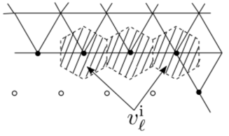
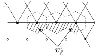
Figure 2. Effective Voronoi cells for the interface nodes (filled circles) are the shaded area in the above figure. Left figure corresponds to METHOD 1, right figure corresponds to METHOD 2. Different choices of effective cells result in different values of weights $\omega^{{\rm i}}_{\ell}$, for method 1, $\omega_{\ell}^{\rm i}=1$, and for method 2, $\omega_{\ell}^{\rm i}<1$ for the outmost interface atoms which are adjacent to the continuum region.

2.3.3. Rank deficiency

Let $I:=\#\Lambda^{i}$ be the number of atoms in the interface and $R:=\#\mathscr{R}$ the number of interacting sites. The number of unknowns $C_{\ell;\rho,\varsigma}$ is then $IR^{2}$. For Method 1, the number of force balance equations is $\frac{1}{2}\#(\Lambda^{\rm i}+\mathscr{R})\times R$, and the number of energy consistency equation is $2IR$. For method 2, we have fewer force balance equations, while the number of constraints for $C_{\ell,\rho,\varsigma}$ is less than $\frac{1}{2}IR^{2}$. It is therefore easy to see that the number of unknowns is much bigger than the number of equations.

2.3.4. Least squares computation of reconstruction parameters

The references [23, 4, 19] construct various examples, where reconstruction parameters can be determined analytically to satisfy the energy and force patch tests (2.8) and (2.9). Instead, we propose to solve them numerically in a preprocessing step.

Comparing the number of equations against the number of free parameters (see §2.3.3), we observe that, if a solution to (2.8) and (2.9) exists, then it cannot be unique. A natural idea, therefore, is to use a least-squares approach,

$$\text{minimize }\sum_{\ell\in\Lambda^{\rm i}}\sum_{\rho,\varsigma\in\mathscr{R}(\ell)}|C_{\ell;\rho,\varsigma}|^{2}\quad\text{ subject to \eqref{eq:E_pt_grac} and \eqref{eq:F_pt_grac}.}$$ (2.10)

We warn from the outset against using (2.10) and explain in § 2.4 that error estimates for QNL type a/c coupling schemes suggest a different selection principle.

Further, in § 2.5, we propose to add a stabilisation mechanism to the interface site potentials that we previously explored in [17]. Our subsequent numerical experiments in § 3 demonstrate that, in general, both of these modifications are required to obtain satisfactory accuracy of the a/c method.

2.4. Consistency and Optimisation of $C_{\ell}$

In [16, Thm. 6.1] it is shown that, under the assumptions that $d=2$ and that the atomistic region $\Omega^{\rm a}$ is connected (and additional natural technical assumptions), any a/c coupling scheme of the type (2.3) satisfying the force and energy patch tests (2.5), (2.6) satisfies a first-order consistency estimate: if $y=y^{\sf B}$ in $\Lambda\setminus\Omega$ and if $\tilde{y}$ is an $H^{2}_{\rm loc}$-conforming interpolant of $y$, then

$$\big{\langle}\delta E(y)-\delta E^{\rm ac}(I_{h}y),u_{h}\big{\rangle}\leq C_{1}\|h\nabla^{2}\tilde{y}\|_{L^{2}(\tilde{\Omega}^{\rm c})},$$ (2.11)

where $C_{1}$ is independent of $y$. (An improved result for a specific variant of GRAC is also proven in [19].)

Of particular interest for the present work is the dependence on $C_{1}$ on the reconstruction parameters $C_{\ell}$, which we can obtain from Equation (6.4) in [16, Thm. 6.1] and a brief calculation:

$$C_{1}\leq C_{1}^{\prime}\,(1+{\rm width}(\Lambda^{\rm i}))\,\sum_{\rho,\varsigma\in\mathscr{R}}|\rho|\,|\varsigma|\,M_{\rho,\varsigma}+C_{1}^{\prime\prime}$$ (2.12)

$$\text{where}\quad M_{\rho,\varsigma}=\max_{\ell\in\Lambda^{\rm i}}\sum_{\tau,\tau^{\prime}\in\mathscr{R}(\ell)}|V_{\tau,\tau^{\prime}}(C_{\ell}\cdot Dy(\ell))|\,|C_{\ell;\tau,\rho}|\,|C_{\ell;\tau^{\prime},\varsigma}|.$$

$C_{1}^{\prime}$ is a generic constant and $C_{1}^{\prime\prime}$ does not depend on the reconstruction parameters.

The estimate (2.12) is of course an overestimation that was convenient for the analysis, whereas intuitively one may think of

$$M(\ell):=\sum_{\rho,\varsigma}|\rho|\,|\varsigma|\sum_{\tau,\tau^{\prime}}\big{|}V_{\tau,\tau^{\prime}}(C_{\ell}\cdot Dy(\ell))\big{|}\,|C_{\ell;\tau,\rho}|\,|C_{\ell;\tau^{\prime},\varsigma}|$$

to be a realistic ($\ell$-dependent) pre-factor. Suppose now that we make the generic structural assumption (see App.B.2 in [18], where this is discussed for an EAM type potential) that $|V_{\tau,\tau^{\prime}}(C_{\ell}\cdot Dy(\ell))|\lesssim\omega(|\tau|)\,\omega(|\tau^{\prime}|)$, where $\omega$ has some decay that is determined by the interaction potential, then we obtain that

$$M(\ell) \lesssim\sum_{\rho,\varsigma}|\rho|\,|\varsigma|\sum_{\tau,\tau^{\prime}}\omega(|\tau|)\,\omega(|\tau^{\prime}|)\,|C_{\ell;\tau,\rho}|\,|C_{\ell;\tau^{\prime},\varsigma}|$$

$$=\Big{(}\sum_{\rho,\tau}|\rho|\omega(|\tau|)|C_{\ell;\tau,\rho}|\Big{)}\,\Big{(}\sum_{\varsigma,\tau^{\prime}}|\varsigma|\omega(|\tau^{\prime}|)|C_{\ell;\tau^{\prime},\varsigma}|\Big{)}$$

$$=\Big{(}\sum_{\rho,\tau}|\rho|\omega(|\tau|)|C_{\ell;\tau,\rho}|\Big{)}^{2}.$$

This indicates that, instead of $\|C\|_{\ell^{2}}$, we should minimise $\max_{\ell\in\Lambda^{\rm i}}\sum_{\rho,\tau}|\rho|\omega(|\tau|)|C_{\ell;\tau,\rho}|$. Since we do not in general know the generic weights $\omega$, we simply drop them, and instead minimise $\sum_{\rho,\tau}|C_{\ell;\tau,\rho}|$. Further, taking the maximum of $\ell\in\Lambda^{\rm i}$ leads to a difficult and computationally expensive multi-objective optimisation problem. Instead, we propose to minimise the $\ell^{1}$-norm of all the coefficients:

$$\text{ minimise }\sum_{\ell\in\Lambda^{\rm i}}\sum_{\rho,\varsigma\in\mathscr{R}(\ell)}|C_{\ell;\rho,\varsigma}|\quad\text{ subject to \eqref{eq:E_pt_grac} and \eqref{eq:F_pt_grac}.}$$ (2.13)

To justify the two rather significant simplifications, we observe that, intuitively, the reconstruction coefficients at different sites should take values of roughly the same order of magnitude. Further, the weight factors coming from the interaction potential should not play a big role since the reconstruction of each “shell” of neighbours is in essence independent of the rest (due to the fact that the reconstruction coefficients must also be valid for potentials with smaller interaction neighbourhood). Finally, we remark that $\ell^{1}$-minimisation tends to generate “sparse” reconstruction parameters which may present some gain in computational cost in the energy and force assembly routines for $E^{\rm ac}$.

2.5. Stability and stabilisation

In order to obtain an energy norm error estimate

$$\|Dy_{h}-Dy\|_{\ell^{2}}\leq C\Big{(}\|h\nabla^{2}\tilde{y}\|_{L^{2}(\tilde{\Omega}^{\rm c})}+\epsilon^{\rm bc}\Big{)},$$ (2.14)

where $\epsilon^{\rm bc}$ is the error due to the artificial boundary condition on $\partial\Omega$, we require a best approximation error estimate, the consistency error estimate (2.11), and most crucially, a stability estimate of the form

$$\langle\delta^{2}E^{\rm ac}(I_{h}y)u_{h},u_{h}\rangle\geq c_{0}\|Du_{h}\|_{\ell^{2}}^{2}$$ (2.15)

for some $c_{0}>0$, indepent of any approximation parameters.

Estimates of the form (2.15) for any form of A/C couplings in dimension greater than one are still poorly understood. We refer to [17, 7, 10] for some preliminary results. For our purposes, the key observations from [17] are the following:

1. There exists no GRAC type a/c coupling for which (2.15) can be expected for general potentials $V$ and general boundary conditions $y_{0}$ even if $y$ itself is stable in the atomistic model.

2. By adding a stabilisation of the from $\kappa|D^{2}y|^{2}$, with $\kappa$ sufficiently large, to the interface region, (2.15) can be expected. (We say “expected” instead of “guaranteed” since the proof of this statement in [17] is restricted to some specific interaction classes.)

Thus, we shall consider also stabilised GRAC type couplings, where the interface site potential is given by

$$\Phi_{\ell}^{\rm i}(y_{h}):=V\big{(}C_{\ell}\cdot Dy_{h}(\ell)\big{)}+\kappa|D_{\rm nn}^{2}y_{h}(\ell)|^{2},$$ (2.16)

where $\kappa\geq 0$ is a stabilisation parameter, and $|D_{\rm nn}^{2}u_{h}(\ell)|^{2}$ is defined as follows: we choose $m\geq d$ linearly independent “nearest-neighbour” directions $b_{1},\dots,b_{m}$ in the lattice, and denote

$$\big{|}D_{\rm nn}^{2}u_{h}(\ell)\big{|}^{2}:=\sum_{j=1}^{m}\big{|}y_{h}(\ell+b_{j})-2y_{h}(\ell)+y_{h}(\ell-b_{j})\big{|}^{2}.$$

The reconstruction parameters $C_{\ell}$ are still determined according to (2.10) or (2.13).

It is straightforward to see that the stabilisation does not generate any ghost forces. That is, if the GRAC part of the potential, $V(C_{\ell}\cdot Dy_{h})$, satisfies the two patch tests (2.5) and (2.6), then the stabilised interface potential $\Phi_{\ell}^{\rm i}$ defined by (2.16) also satisfies both patch tests.

3. Numerical Tests

3.1. Model problems

Our implementation is for the 2D triangular lattice ${\sf A}\mathbb{Z}^{2}$ defined by

$${\sf A}=\begin{pmatrix}1&\cos(\pi/3)\\ 0&\sin(\pi/3)\end{pmatrix}.$$

To generate a defect, we remove $k$ atoms

$$\left\{\begin{array}[]{rl}\Lambda^{\rm def}_{k}:=\big{\{}-(k/2+1)e_{1},\dots,k/2e_{1}\big{\}},&\text{ if $k$ is even, }\\[2.84526pt] \Lambda^{\rm def}_{k}:=\big{\{}-(k-1)/2e_{1},\dots,(k-1)/2e_{1}\big{\}},&\text{ if $k$ is odd,}\end{array}\right.$$

to obtain $\Lambda:={\sf A}\mathbb{Z}^{2}\setminus\Lambda^{\rm def}_{k}$. For small $k$, the defect acts like a point defect, while for large $k$ it acts like a small crack embedded in the crystal. In our experiments we shall consider $k=2,11$.

We choose an elongated hexagonal domain $\Omega^{\rm a}$ containing $K$ layers of atoms surrounding the vacancy sites and the full computational domain $\Omega$ to be an elongated hexagon containing $N$ layers of atoms surrounding the vacancy sites; see Figure 1(c) for an illustration. The domain parameters are chosen so that $N\approx K^{2}$. The finite element mesh is graded so that the mesh size function $h(x)={\rm diam}(T)$ for $T\in\mathscr{T}_{h}$ satisfies $h(x)\approx(|x|/K)^{3/2}$. These choices balance the coupling error at the interface, the finite element interpolation error and the far-field truncation error [5, Sec.5.2]. One then obtains [5, Prop. 5.5] under additional conditions on the stability of the method and the magnitude of the reconstruction parameters (we can verify both only a posteriori) that

$$\|\nabla y-\nabla y_{h}\|_{L^{2}}\leq C{\rm DOF}^{-1},$$ (3.1)

where $y$ is identified with its P1 interpolant on the canonical triangulation of $\Lambda$ and ${\rm DOF}$ denotes the total number of degrees of freedom (i.e. the number of atomistic sites $\Lambda^{{\rm a},{\rm i}}$ plus the number of finite element nodes).

The site energy is given by an EAM (toy-)model (2.1), with

$$\phi(r)=[e^{-2a(r-1)}-2e^{-a(r-1)}],\quad\psi(r)=e^{-br},$$

$$F(\tilde{\rho})=c\big{[}(\tilde{\rho}-\tilde{\rho}_{0})^{2}+(\tilde{\rho}-\tilde{\rho}_{0})^{4}\big{]},$$

with parameters $a=4.4,b=3,c=5,\tilde{\rho}_{0}=6e^{-b}$. The interaction range is $\mathscr{N}(\ell)=\Lambda\cap B_{2}(\ell)$, i.e., next nearest neighbors in hopping distance.

3.1.1. Di-vacancy

In the di-vacancy test two neighboring sites are removed, i.e., $k=2$. We apply $3\%$ isotropic stretch and $3\%$ shear loading, by setting

$${\sf B}:=\begin{pmatrix}1+s&\gamma_{\rm II}\\ 0&1+s\end{pmatrix}\cdot{\sf F}_{0}.$$

where ${\sf F}_{0}\propto I$ minimizes $W$, $s=\gamma_{\rm II}=0.03$.

3.1.2. Micro-crack

In the microcrack experiment, we remove a longer segment of atoms, $\Lambda^{\rm def}_{11}=\{-5e_{1},\dots,5e_{1}\}$ from the computational domain. The body is then loaded in mixed mode ${\rm I}$ & ${\rm II}$, by setting,

$${\sf B}:=\begin{pmatrix}1&\gamma_{\rm II}\\ 0&1+\gamma_{\rm I}\end{pmatrix}\cdot{\sf F}_{0}.$$

where ${\sf F}_{0}\propto I$ minimizes $W$, and $\gamma_{\rm I}=\gamma_{\rm II}=0.03$ ($3\%$ shear and $3\%$ tensile stretch).

3.2. Methods

We shall test the GRAC variants METHOD 1, METHOD 2 with both least squares solution (2.10) and $\ell^{1}$-minimisation (2.13) to solve for the reconstruction parameters, and with stabilisation parameters $\kappa=0,1$. The resulting methods are denoted by M$i$-L$p$-S$\kappa$, where $i\in\{1,2\}$, $p\in\{2,1\}$, $\kappa\in\{0,1\}$.

Some additional practical details for the implementation of METHOD 1 and METHOD 2 are described in Appendix 5.2.

We compare the GRAC methods with the five competitors previously considered in [8, 12]:

• ATM: full atomistic model is minimized with the constraint $y=y^{\sf B}$ in $\Lambda\setminus\Omega$; see also [5, Sec. 4.1].

• QCE: original quasicontinuum method without ghost-force correction [15].

• B-QCE, B-QCE+: blended quasicontinuum method, implementation based on [12]; B-QCE+ is a variant with highly optimised approximation parameters described in [8, Sec. 4.3].

• QCF: sharp-interface force-based a/c coupling [3], formally equivalent to the quasi-continuum method with ghost-force correction [22].

• B-QCF: blended force-based a/c coupling, as described in [8].

3.3. Results

Following [12, 8] we present two experiments, a di-vacancy ($k=2$) and a “micro-crack” ($k=11$). In the first experiment, we are able to clearly observe the asymptotic behaviour of the a/c coupling schemes predicted in (3.1), while in the second experiment we observe a significant pre-asymptotic regime where the prediction (3.1) becomes relevant only at fairly high DOF.

For both experiments we plot the absolute errors against the number of degrees of freedom (DOF), which is propoertional to computational cost, in the $H^{1}$-seminorm, the $W^{1,\infty}$-seminorm and in the (relative) energy.

The results are shown in Figures 3, 4 and 5 for the divacancy problem and in Figures 6, 7 and 8 for the micro-crack problem.

3.3.1. Effect of $\ell^{1}$-minimisation

In all error graphs we observe that computing the reconstruction coefficients via least-squares ($\ell^{2}$-minimisation) leads to large errors in the computed solution and likely even lack of convergence. Stabilisation does not remedy this, which indicates that the issue indeed lies in the consistency error. By contrast, using (2.13) ($\ell^{1}$-minimisation) to compute the reconstruction parameters leads to errors that are competitive with the provably quasi-optimal schemes QCF and B-QCF.

3.3.2. Effect of stabilisation

If no stabilisation is used ($\kappa=0$), then all error graphs display large errors in a pre-asymptotic regime and in some cases, most pronounced in Figure 7, non-monotone convergence history.

Adding the stabilisation by setting $\kappa=1$ the $H^{1}$ and $W^{1,\infty}$ errors are reduced in both examples, indeed significantly so in the important pre-asymptotic regime, and the oscillations in the convergence history are removed. With stabilisation the convergence rates predicted in [5, Sec. 5.2] are clearly observed.

3.3.3. Comparison of a/c couplings

In all error graphs we clearly observe the optimal convergence rate of GRAC (M$i$-L1-S1 variants) among the tested energy-based methods (ATM, QCE, B-QCE, B-QCE+, GRAC). Indeed, the errors are even competitive with the quasi-optimal force-based schemes (QCF, B-QCF): for $H^{1}$ errors they are essentially comparable, for $W^{1,\infty}$ errors the force-based schemes are only better by a moderate constant factor, while for the energy errors the GRAC methods are optimal. (Note that, for QCF we evaluate the QCE energy and for B-QCF we evaluate the B-QCE energy.)

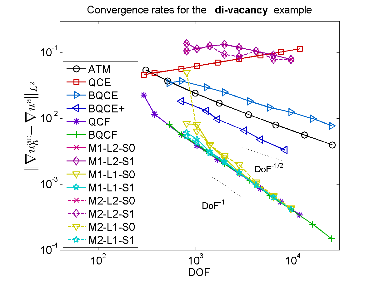
Figure 3. Convergence rates in the energy-norm (the $H^{1}$-seminorm) for the divacancy benchmark problem described in Section § 3.1.1 .

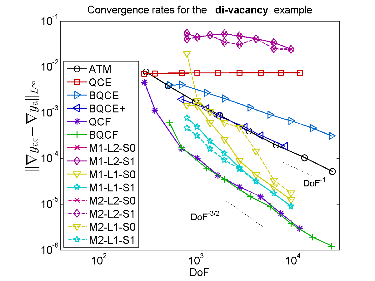
Figure 4. Convergence rates in the $W^{1,\infty}$-seminorm for the divacancy benchmark problem described in Section § 3.1.1 .

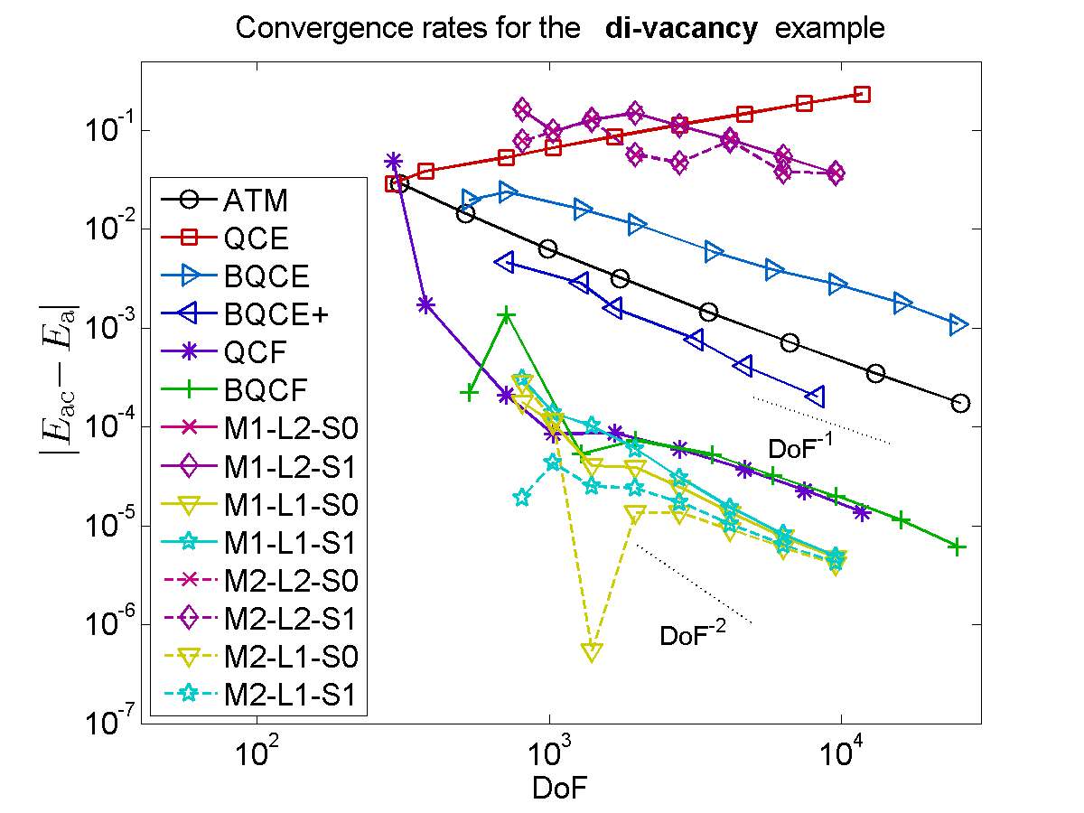
Figure 5. Convergence rates in the relative energy for the divacancy benchmark problem described in Section § 3.1.1 .

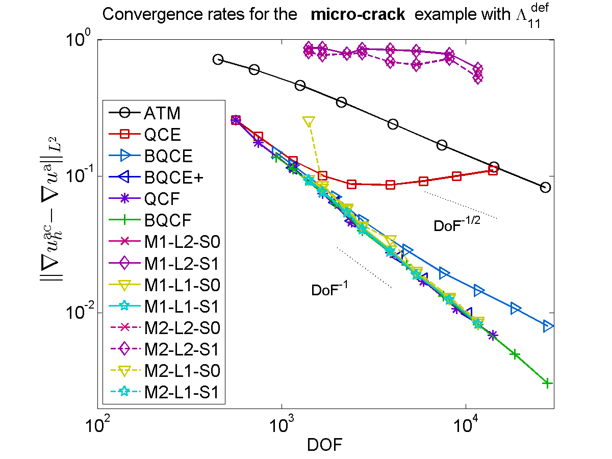
Figure 6. Convergence rates in the energy-norm (the $H^{1}$-seminorm) for the microcrack benchmark problem with $\Lambda^{\rm def}_{11}$ described in Section § 3.1.2 .

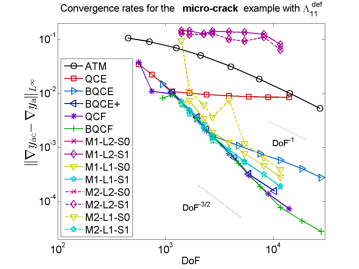
Figure 7. Convergence rates in the $W^{1,\infty}$-seminorm for the microcrack benchmark problem with $\Lambda^{\rm def}_{11}$ described in Section § 3.1.2 .

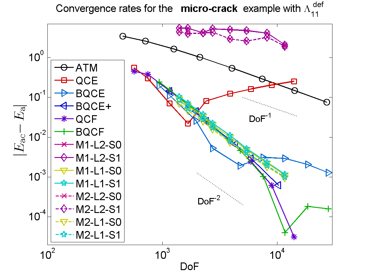
Figure 8. Convergence rates in the relative energy for the microcrack benchmark problem with $\Lambda^{\rm def}_{11}$ described in Section § 3.1.2 .

4. Conclusion

We have succeeded in presenting the first patch test consistent energy-based atomistic-to-continuum coupling formulation, GRAC, which is applicable to general a/c interface geometries and general (short-ranged) many-body interactions, and demonstrated its potential in a 2D implementation.

We have discussed the critical issues of $\ell^{1}$-minimisation and of stabilisation, and have demonstrated that our final formulations yield an energy-based a/c coupling that is optimal among the energy-based methods we tested, which represent a fairly generic sample, and are even competitive compared against the quasi-optimal force-based coupling schemes.

While the construction of the GRAC scheme is involved, it has the advantage that no additional approximation parameters (e.g., the blending function $\beta$ in the B-QCE and B-QCF schemes [12, 8]) must be adapted to the problem at hand.

The main challenge that requires additional work is the complexity of the precomputation of the reconstruction parameters, which may become prohibitive for wider interaction stencils, in particular in 3D. It may then become necessary to make further simplifications such as the ones we made in METHOD 2, in order to substantially reduce the computational cost and storage to compute these parameters.

From a theoretical perspective the main open problem is to prove that the geometric consistency equations (2.8) and (2.9) always have at least one solution. We can, at present, provide no analytical evidence to support this claim, however, we have so far not encountered a situation where a solution could not be computed numerically.

Finally, we remark that the consistency of the GRAC scheme is still not entirely settled. First-order consistency is only proven in 1D and in 2D under the restrictive assumption that the atomistic region is connected [16, 25].

5. Appendix

5.1. First variation of $E^{\rm ac}$

The following calculations provide the details for the computation of $\delta E^{\rm ac}$ in § 2.3.2.

5.1.1. Atomistic component

$$\langle\delta E^{\rm a},u\rangle= \sum_{\ell\in\Lambda^{{\rm a}}}\sum_{\rho\in\mathscr{R}}\nabla_{\rho}VD_{\rho}u(\ell)$$

$$= \sum_{\ell\in\Lambda^{{\rm a}}}\sum_{\rho\in\mathscr{R}^{+}}\nabla_{\rho}V(u(\ell+\rho)-u(\ell))+\nabla_{-\rho}V(u(\ell-\rho)-u(\ell))$$

$$= \sum_{\ell\in\Lambda^{{\rm a}}}\sum_{\rho\in\mathscr{R}^{+}}\nabla_{\rho}V(u(\ell+\rho)-u(\ell-\rho))$$

$$= \sum_{\ell+\rho\in\Lambda^{{\rm a}},\rho\in\mathscr{R}^{+}}\big{[}\nabla_{\rho}V\cdot u(\ell)\big{]}-\sum_{\ell-\rho\in\Lambda^{{\rm a}},\rho\in\mathscr{R}^{+}}\big{[}\nabla_{\rho}V\cdot u(\ell)\big{]}$$

5.1.2. Interface component

$$\langle\delta E^{\rm i},u\rangle= \sum_{\ell\in\Lambda^{{\rm i}}}\omega_{\ell}^{\rm i}\langle\delta V\big{(}(\sum_{\varsigma\in\mathscr{R}}C_{\ell;\rho,\varsigma}D_{\varsigma}y(\ell))_{\rho\in\mathscr{R}}\big{)},u\rangle$$

$$= \sum_{\ell\in\Lambda^{{\rm i}}}\omega_{\ell}^{\rm i}\sum_{\rho\in\mathscr{R}}\sum_{\varsigma\in\mathscr{R}}C_{\ell;\rho,\varsigma}\nabla_{\rho}VD_{\varsigma}u(\ell)$$

$$= \sum_{\ell\in\Lambda^{{\rm i}}}\omega_{\ell}^{\rm i}\sum_{\rho\in\mathscr{R}^{+}}\sum_{\varsigma\in\mathscr{R}}(C_{\ell;\rho,\varsigma}-C_{\ell;-\rho,\varsigma})\nabla_{\rho}V(u(\ell+\varsigma)-u(\ell))$$

$$= \sum_{\ell-\varsigma\in\Lambda^{{\rm i}},\varsigma\in\mathscr{R}}\omega_{\ell-\varsigma}^{\rm i}\sum_{\rho\in\mathscr{R}^{+}}(C_{\ell-\varsigma;\rho,\varsigma}-C_{\ell-\varsigma;-\rho,\varsigma})\big{[}\nabla_{\rho}V\cdot u(\ell)\big{]}$$

$$-\sum_{\ell\in\Lambda^{{\rm i}}}\omega_{\ell}^{\rm i}\sum_{\rho\in\mathscr{R}^{+}}\sum_{\varsigma\in\mathscr{R}}(C_{\ell;\rho,\varsigma}-C_{\ell;-\rho,\varsigma})\big{[}\nabla_{\rho}V\cdot u(\ell)\big{]}$$

5.1.3. Cauchy–Born component

$$\langle\delta E^{\rm c},u\rangle= \sum_{T}v_{T}\langle\delta W,u\rangle$$

$$= \sum_{T}\frac{v_{T}}{|\rm vor|}\langle\delta V\big{(}(\nabla_{T}y\cdot\rho)_{\rho\in\mathscr{R}}\big{)},u\rangle$$

$$= \sum_{T}\frac{v_{T}}{|\rm vor|}\sum_{\rho\in\mathscr{R}}\nabla_{\rho}V\nabla_{T}u\cdot\rho$$

$$= \sum_{T}\frac{v_{T}}{|\rm vor|}\sum_{\rho\in\mathscr{R}}\nabla_{\rho}V\sum_{i=1}^{3}u^{T}_{i}\nabla_{T}\phi_{i}^{T}\cdot\rho$$

$$= \sum_{T}\frac{v_{T}}{|\rm vor|}\sum_{\rho\in\mathscr{R}^{+}}2\nabla_{\rho}V\sum_{i=1}^{3}u^{T}_{i}\nabla_{T}\phi_{i}^{T}\cdot\rho$$

$$= \sum_{T}\sum_{\rho\in\mathscr{R}^{+}}\sum_{i=1}^{3}2\frac{v_{T}}{|\rm vor|}\nabla_{T}\phi_{i}^{T}\cdot\rho\big{[}\nabla_{\rho}V\cdot u^{T}_{i}\big{]}$$

5.2. Setup of the geometric consistency equations

We now introduce additional details for implementing the GRAC formulation in (2.3). This gives further concrete details on how to setup the geometric consistency equations (2.8) and (2.9) specifically for the triangular lattice. The process that we propose is, however, more generally applicable. Here, the interface region is $r$ layers of atoms around $\Lambda^{\rm a}$, and $r$ is the radius of interaction range $\mathscr{R}$ in terms of hopping distance. We describe the process only for METHOD 1, as the one for METHOD 2 is very similar.

To satisfy the force patch test consistency equation, in the nearest neighbor case we considered in [19] we take the following strategy, where the reconstruction parameters $C_{\ell}$ are extended to $\Lambda\setminus\Lambda^{\rm i}$ by

$$C_{\ell}=\left\{\begin{array}[]{rl}C^{\rm a},&\ell\in\Lambda^{\rm a},\\ C^{\rm c},&\ell\in\Lambda\setminus\Lambda^{{\rm a},{\rm i}},\end{array}\right.$$

Define the six nearest-neighbour lattice directions by $a_{1}:=(1,0)$, and $a_{j}:={\sf Q}_{6}^{j-1}a_{1}$, $j\in\mathbb{Z}$, where ${\sf Q}_{6}$ denotes the rotation through angle $2\pi/6$ and we note that $a_{j+3}=-a_{j}$. Then $C^{\rm a}$ is given by $C^{\rm a}_{i,j}=\delta_{i,j}$, $C^{\rm c}$ is given by $C^{\rm c}_{i,j}=\frac{2}{3}\delta_{i,j}+\frac{1}{3}\delta_{i,j+1}+\frac{1}{3}\delta_{i,j-1}$, $i,j=1,\dots,6$, where $\delta$ is the Kronecker delta function.

The argument employed in [19, Lemma 3.2] can be extended to longer range interactions. There exist matrices $C_{\ell}^{\rm c}$ such that, upon defining $\Psi_{\ell}(y):=V(C_{\ell}^{\rm c}\cdot Dy(\ell))$, we have

$$\langle\delta\Psi_{\ell}({\sf F}x),v\rangle=\int_{{\rm vor}(\ell)}\partial W({\sf F}):\nabla v(x)\,{\rm d}x\qquad\forall\ell\in\Lambda\cap\Omega^{\rm c},$$ (5.1)

that is, under uniform deformation, the forces generated by the Cauchy–Born site potential $\int_{{\rm vor}(\ell)}W(\nabla y)\,{\rm d}x$ are the same as those of $\Phi_{\ell}$.

Carrying this out in practise requires that several layers of atoms surrounding $\Lambda^{{\rm a},{\rm i}}$, denoted by $\Lambda^{\rm c}$, coincide with the finite element nodes in that region. Upon choosing $\mathscr{T}_{\mu}$ to be a uniform partition over $\Lambda^{\rm c}$, these parameters can be computed analytically. The details are shown in Appendix 5.3 for next nearest neighbor interactions.

Upon defining the coefficients for the atomistic and continuum region, we can use Proposition 2.3.2 to compute unknown parameters $C_{\ell;\rho,\varsigma}$.

5.3. Determination of the coefficients $C^{\rm c}$ for next nearest neighbor interaction.

We now calculate the coefficients $C^{\rm c}$ from the equation (5.1). On the canonical triangular mesh induced by $\Lambda$, let

$$V^{\rm c}_{\ell}=\frac{1}{6}\sum_{T\owns\ell}V(D_{T}u)$$

be the Cauchy-Born site energy with respect to $\ell\in\Lambda$. As the six nearest-neighbour lattice directions are defined in Section 5.2. The second nearest-neighbour lattice directions can be expressed as $a_{2j+5}=2a_{j}$, $a_{2j+6}=a_{j}+a_{\rm shift(j)}$, $j=1,\dots,6$, , where $\rm shift\{1,2,3,4,5,6\}=\{2,3,4,5,6,1\}$. Therefore $a_{j}$’s, $j=1,\dots,18$ form the the interaction range $\mathscr{R}$ for next nearest neighbor interactions.

$V_{\ell}^{\rm c}$ only depends on the first 6 variables $D_{i}y$ of $V$, a direct calculation shows that

$$\partial_{1}V_{\ell}^{\rm c}=\frac{1}{3}\partial_{2}V+\frac{2}{3}\partial_{1}V+\frac{1}{3}\partial_{6}V+\frac{2}{3}\partial_{9}V+\frac{2}{3}\partial_{9}V+\partial_{8}V+\frac{4}{3}\partial_{7}V+\partial_{18}V+\frac{2}{3}\partial_{17}V$$

and similiarly for $\partial_{i}V_{\ell}^{\rm c}$ with $i=2,\dots,6$.

Now we can write down the modified potential $\Psi_{\ell}$ defined in (5.1), which generate the same force for arbitrary uniform deformations. In the following expression of $\Psi_{\ell}$, for $i=1,\dots,6$, $D_{i}y$ are abbreviated by $D_{i}$,

$$\Psi_{\ell}= V\big{(}\frac{2}{3}D_{1}+\frac{1}{3}D_{2}+\frac{1}{3}D_{6},\frac{2}{3}D_{2}+\frac{1}{3}D_{1}+\frac{1}{3}D_{3},\frac{2}{3}D_{3}+\frac{1}{3}D_{2}+\frac{1}{3}D_{4},$$

$$\frac{2}{3}D_{4}+\frac{1}{3}D_{3}+\frac{1}{3}D_{5},\frac{2}{3}D_{5}+\frac{1}{3}D_{4}+\frac{1}{3}D_{6},\frac{2}{3}D_{6}+\frac{1}{3}D_{5}+\frac{1}{3}D_{1},$$

$$\frac{4}{3}D_{1}+\frac{2}{3}D_{2}+\frac{2}{3}D_{6},D_{1}+D_{2},\frac{4}{3}D_{2}+\frac{2}{3}D_{1}+\frac{2}{3}D_{3},$$

$$D_{2}+D_{3},\frac{4}{3}D_{3}+\frac{2}{3}D_{2}+\frac{2}{3}D_{4},D_{3}+D_{4}$$

$$\frac{4}{3}D_{4}+\frac{2}{3}D_{3}+\frac{2}{3}D_{5},D_{4}+D_{5},\frac{4}{3}D_{5}+\frac{2}{3}D_{4}+\frac{2}{3}D_{6},$$

$$D_{5}+D_{6},\frac{4}{3}D_{6}+\frac{2}{3}D_{5}+\frac{2}{3}D_{1},D_{6}+D_{1}\big{)}$$

Hence the coefficients $C_{\ell}^{\rm c}$ can be drawn from above expression by using $\Psi_{\ell}=V(C_{\ell}^{\rm c}\cdot Dy(\ell))$.

References

- [1] M. S. Daw and M. I. Baskes. Embedded-Atom Method: Derivation and Application to Impurities, Surfaces, and other Defects in Metals. Physical Review B, 20, 1984.
- [2] M. Dobson and M. Luskin. An optimal order error analysis of the one-dimensional quasicontinuum approximation. SIAM Journal on Numerical Analysis, 47(4):2455–2475, 2009.
- [3] M. Dobson, M. Luskin, and C. Ortner. Stability, instability, and error of the force-based quasicontinuum approximation. Arch. Ration. Mech. Anal., 197(1):179–202, 2010.
- [4] W. E, J. Lu, and J. Z. Yang. Uniform accuracy of the quasicontinuum method. Phys. Rev. B, 74(21):214115, 2006.
- [5] V. Ehrlacher, C. Ortner, and A. V. Shapeev. Analysis of boundary conditions for crystal defect atomistic simulations. ArXiv e-prints, 1306.5334, 2013.
- [6] H. Fischmeister, H. Exner, M.-H. Poech, S. Kohlhoff, P. Gumbsch, S. Schmauder, L. S. Sigi, and R. Spiegler. Modelling fracture processes in metals and composite materials. Z. Metallkde., 80:839–846, 1989.
- [7] X. Li, M. Luskin, and C. Ortner. Positive-definiteness of the blended force-based quasicontinuum method. Multiscale Model. Simul., 10, 2012.
- [8] X. Li, M. Luskin, C. Ortner, and A. Shapeev. Theory-based benchmarking of the blended force-based quasicontinuum method. Comput. Methods Appl. Mech. Engrg., to appear, 2013.
- [9] J. Lu and P. Ming. Convergence of a force-based hybrid method for atomistic and continuum models in three dimension. arXiv:1102.2523.
- [10] J. Lu and P. Ming. Stability of a force-based hybrid method in three dimension with sharp interface. ArXiv e-prints, 1212.3643, 2012.
- [11] M. Luskin and C. Ortner. Atomistic-to-continuum-coupling. Acta Numerica, 2013.
- [12] M. Luskin, C. Ortner, and B. Van Koten. Formulation and optimization of the energy-based blended quasicontinuum method. Comput. Methods Appl. Mech. Engrg., 253, 2013.
- [13] C. Makridakis, D. Mitsoudis, and P. Rosakis. On atomistic-to-continuum couplings without ghost forces in three dimensions. ArXiv e-prints, 1211.7158, 2012.
- [14] P. Ming and J. Z. Yang. Analysis of a one-dimensional nonlocal quasi-continuum method. Multiscale Modeling & Simulation, 7(4):1838–1875, 2009.
- [15] M. Ortiz, R. Phillips, and E. B. Tadmor. Quasicontinuum analysis of defects in solids. Philosophical Magazine A, 73(6):1529–1563, 1996.
- [16] C. Ortner. The role of the patch test in 2D atomistic-to-continuum coupling methods. ESAIM Math. Model. Numer. Anal., 46, 2012.
- [17] C. Ortner, A. Shapeev, and L. Zhang. (in-)stability and stabilisation of qnl-type atomistic-to-continuum coupling methods. ArXiv e-prints, 1308.3894, 2013.
- [18] C. Ortner and F. Theil. Justification of the cauchy–born approximation of elastodynamics. Arch. Ration. Mech. Anal., 207, 2013.
- [19] C. Ortner and L. Zhang. Construction and sharp consistency estimates for atomistic/continuum coupling methods with general interfaces: a 2D model problem. SIAM J. Numer. Anal., 50, 2012.
- [20] A. V. Shapeev. Consistent energy-based atomistic/continuum coupling for two-body potential: 1D and 2D case. arXiv:1010.0512, to appear in SIAM MMS.
- [21] A. V. Shapeev. Consistent energy-based atomistic/continuum coupling for two-body potentials in three dimensions. SIAM J. Sci. Comput., 34(3):B335–B360, 2012.
- [22] V. B. Shenoy, R. Miller, E. B. Tadmor, D. Rodney, R. Phillips, and M. Ortiz. An adaptive finite element approach to atomic-scale mechanics–the quasicontinuum method. J. Mech. Phys. Solids, 47(3):611–642, 1999.
- [23] T. Shimokawa, J. J. Mortensen, J. Schiotz, and K. W. Jacobsen. Matching conditions in the quasicontinuum method: Removal of the error introduced at the interface between the coarse-grained and fully atomistic region. Phys. Rev. B, 69(21):214104, 2004.
- [24] S. P. Xiao and T. Belytschko. A bridging domain method for coupling continua with molecular dynamics. Comput. Methods Appl. Mech. Engrg., 193(17-20):1645–1669, 2004.
- [25] L. Zhang. Patch test consistency implies first order consistency: Atomistic/continuum coupling in 3d. Work in progress.