Nuclear vorticity in isoscalar E1 modes: Skyrme-RPA analysis

Abstract

Two basic concepts of nuclear vorticity, hydrodynamical (HD) and Rawenthall-Wambach (RW), are critically inspected. As a test case, we consider the interplay of irrotational and vortical motion in isoscalar electric dipole E1(T=0) modes in ²⁰⁸Pb, namely the toroidal and compression modes. The modes are described in a self-consistent random-phase-approximation (RPA) with the Skyrme force SLy6. They are examined in terms of strength functions, transition densities, current fields, and formfactors. It is shown that the RW conception (suggesting the upper component of the nuclear current as the vorticity indicator) is not robust. The HD vorticity is not easily applicable either because the definition of a velocity field is too involved in nuclear systems. Instead, the vorticity is better characterized by the toroidal strength which closely corresponds to HD treatment and is approximately decoupled from the continuity equation.

I Introduction

It is well known that the nuclear flow may be both irrotational and vortical Bohr_book_74 ; Ring_book_80 . The irrotational motion is presented by numerous examples of low-energy excitations and electric giant resonances (GR) Harakeh_book_01 while the vortical motion is exhibited by single-particle excitations Ra87 , nuclear rotation Bohr_book_74 , and particular GR (toroidal electric dipole Dub_75_83 ; Sem81 and twist magnetic quadrupole HE_77 ; HE_79 ).

Collective nuclear vorticity in electric GR is especially interesting. Though multipole electric GR are most irrotational, there is a remarkable exception in the isoscalar E1(T=0) channel. Here, after exclusion of the nuclear center-of-mass (c.m.) motion, the vortical toroidal mode (TM) dominates in the low-energy (E$<$ 10 MeV) E1(T=0) excitations Pa07 ; Kva_PRC_11 . So, in this channel, the nuclear vorticity is realized as a leading mode. It is remarkable that the TM lies in the energy region of so called pygmy dipole resonance (PDR) and determines there the main flow Ry02 ; Rep_PRC_13 . The low-energy strength (LES) in this region is of high current interest as it can deliver useful information on principle nuclear properties (nuclear symmetry energy, neutron skin) with consequences to various astrophysical applications Pa07 . The vorticity can affect these relations and thus deserves detailed analysis.

Despite some previous studies (see e.g. Ra87 ; Sem81 ; Se83 ; Ca99 ), our knowledge about the nuclear vorticity is still poor. Even the basic points, the definition of nuclear vorticity and choice of the proper observable, are disputable. In hydrodynamics (HD), the vorticity is defined as a curl of the velocity Lan87 ,

$$\vec{\varpi}({\vec{r}})=\vec{\nabla}\times\vec{v}(\vec{r})\;.$$ (1)

However, nuclear physics deals not with velocities but nuclear currents. In this connection, Raventhall and Wambach have proposed the $j_{+}(r)$-component of the nuclear current as an indicator of the vorticity (RW vorticity in what follows) Ra87 . Indeed, $j_{+}(r)$ may be posed as unrestricted by the continuity equation (CE)

$$\delta\dot{\rho}_{\nu}(\vec{r})+\vec{\nabla}\cdot\delta\vec{j}_{\nu}(\vec{r})=0$$ (2)

(where $\delta\rho_{\nu}$ and $\delta\vec{j}_{\nu}$ are nucleon and current transition densities for excited states $\nu$) and thus suitable for a divergence-free (vortical) observable Ra87 ; Ca99 ; Hei_PRC_82 . However, HD and RW definitions of the vorticity strictly contradict each other Kva_PRC_11 when being applied to the E1(T=0) compression mode (CM) Har_PRL_77 ; Stri82 . Following HD, the CM velocity field is

$$\vec{v}_{\text{CM}}(\vec{r})\propto\vec{\nabla}\,(r^{3}Y_{1\mu})$$ (3)

and so this mode is fully irrotational. At the same time, the CM has an essential $j_{+}(r)$-contribution Kva_PRC_11 and so, following RW, is of a mixed (vortical/irrotational) character. This discrepancy certainly needs a careful analysis.

The aim of the present paper is to scrutinize the HD and RW prescriptions and finally propose the most relevant indicator and measure of the nuclear vorticity. As shown below, the RW prescription is not accurate and may result in wrong conclusions, like in the CM case mentioned above. The HD prescription (1) is more physically transparent but not convenient for practical use in nuclear physics. Instead, the toroidal strength seems to be the most appropriate (though not perfect) measure of nuclear vorticity in internal single-particle and collective excitations. Toroidal strength can be considered as approximate HD treatment in practicable form. It provides sufficiently good decoupling from CE (2), avoids shortcomings of the RW prescription, and exhibits a natural curl-like vortical motion.

Our analysis uses TM and CM as most relevant representatives of the vortical and irrotational flows. Schematic images of these modes in E1(T=0) channel are presented in Fig. 1. Note that the TM and CM operators are related Kva_PRC_11 . Both modes dominate the E1(T=0) channel and their maxima are well separated in energy.

The calculations are performed for ²⁰⁸Pb within the Skyrme random-phase-approximation (RPA) approach Rei92 . The method is fully self-consistent in the sense that both the mean field and residual interaction are derived from the Skyrme functional Skyrme ; Vau72 ; En75 ; Ben03 . The residual interaction takes into account all the terms of the Skyrme functional as well as the Coulomb (direct and exchange) terms. The Skyrme force SLy6 Sly6 , well describing the isovector (T=1) giant dipole resonance (GDR) in heavy nuclei nest_PRC_08 , is used. This study is a continuation of our previous exploration of TM, CM, and RW strengths Kva_PRC_11 within the self-consistent separable random-phase-approximation (SRPA) method nest_PRC_02 ; nest_PRC_06 . The present Skyrme RPA approach does not use any separable approximation and implements a wider configuration space.

A large set of dynamical characteristics is analyzed. Not only strength functions but also current/velocity fields, and formfactors are considered. What is important, curls and divergences of TM and CM flows, as their natural signatures, are inspected. These characteristics are refined from the dominant Tassie collective modes (e.g. GDR or spurious center of mass motion) whose curls and divergences are zero by definition. At the same time, curls and divergences are effective fingerprints of vortical TM and irrotational CM, which are not the Tassie modes.

The paper is organized as follows. In Sec. II, the basic formalism for TM/CM modes and RW/HD vorticity prescriptions is presented. In Sec. III, the calculation scheme is outlined and the dynamical characteristics to be explored (strength functions, curent/velocity fields) are defined. In Sec. IV, the numerical results are presented. In Sec. V, various prescriptions of the vorticity are discussed. The toroidal strength is shown to be the most robust measure of the vorticity. In Sec. VI, the summary is done.

II Theoretical background

II.1 Basic expressions

The standard electrical multipole operator reads BMv1 :

$$\hat{M}(E\lambda\mu,k) = -i\frac{(2\lambda+1)!!}{ck^{\lambda+1}(\lambda+1)}$$

$$\cdot\int\!d^{3}r\hat{\vec{j}}_{\text{nuc}}(\vec{r})\!\cdot\![\vec{\nabla}\!\times\!(\vec{r}\!\times\!\vec{\nabla})j_{\lambda}(kr)Y_{\lambda\mu}(\hat{\vec{r}})]$$

$$= \frac{(2\lambda+1)!!}{ck^{\lambda+1}}\sqrt{\frac{\lambda}{\lambda+1}}$$

$$\cdot\int d^{3}r\>[\>j_{\lambda}(kr)\>\vec{Y}_{\lambda\lambda\mu}(\hat{\vec{r}})\>]\cdot[\vec{\nabla}\times\hat{\vec{j}}_{\text{nuc}}(\vec{r})]$$

where $\hat{\vec{j}}_{\rm{nuc}}(\vec{r})=\hat{\vec{j}}_{\rm{c}}(\vec{r})+\hat{\vec{j}}_{\rm{m}}(\vec{r})$ is operator of the nuclear current density consisting from the convection and magnetization parts; $j_{\lambda}(kr)$ is the spherical Bessel function; $\vec{Y}_{\lambda\lambda\pm 1\mu}(\hat{\vec{r}})$ and $Y_{\lambda\mu}(\hat{\vec{r}})$ are vector and ordinary spherical harmonics Va76 . Following Kva_PRC_11 , the role of the magnetization current $\hat{\vec{j}}_{\text{m}}(\vec{r})$ in E1(T=0) channel is negligible. So only the convection current $\hat{\vec{j}}_{\text{c}}(\vec{r})$ is further involved. For the sake of brevity, we will skip below (up to the cases of a possible confusion) the coordinate dependence in currents, densities and spherical harmonics.

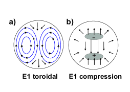
Figure 1: (a) Schematic view of the E1(T=0) toroidal (a) and compression (b) modes Rep_PRC_13 . The driving field is directed along z-axis. The arrows indicate the flow directions but not the strengths. In the panel (b), the compression (+) and decompression (–) regions, characterized by increased and decreased density, are marked.

In the long-wave approximation ($k\to 0$), we get

$$\hat{M}(E\lambda\mu,k)\approx\hat{M}(E\lambda\mu)+k\>\hat{M}_{\text{TM}}(E\lambda\mu)$$ (5)

where

$$\hat{M}(E\lambda\mu) = -\frac{i}{kc}\int d^{3}r\>(\vec{\nabla}\cdot\hat{\vec{j}}_{\text{c}})r^{\lambda}Y_{\lambda\mu}$$ (6)

$$= -\int d^{3}r\>\hat{\rho}\>r^{\lambda}Y_{\lambda\mu}$$

is the familiar electric operator (with $\hat{\rho}$ being the density operator) and

$$\hat{M}_{\text{TM}}(E\lambda\mu) = \frac{i}{2c(\lambda+1)(2\lambda+3)}$$ (8)

$$\cdot\int d^{3}r\hat{\vec{j}}_{\text{c}}\cdot[\>\vec{\nabla}\times\>(\vec{r}\times\vec{\nabla})r^{\lambda+2}Y_{\lambda\mu}]$$

$$= -\frac{1}{2c}\sqrt{\frac{\lambda}{\lambda+1}}\,\frac{1}{2\lambda+3}\int d^{3}r\>r^{\lambda+2}\vec{Y}_{\lambda\lambda\mu}$$

$$\cdot\left(\vec{\nabla}\times\hat{\vec{j}}_{\text{c}}\right)$$

is the toroidal operator Dub_75_83 ; Sem81 ; Kva_PRC_11 ; Kv03 . This operator is the second order ($\sim k^{2}$) correction to the dominant electric operator (6). It becomes dominant at $k\gg 0$. Being determined by the curl $\left(\vec{\nabla}\times\hat{\vec{j}}_{\text{c}}\right)$, the toroidal flow is well (though not exactly, see discussion in Sec. IV-D) decoupled from CE. For this reason the toroidal operator cannot be presented through the nuclear density alone and needs knowledge of the current distribution.

The CM operator reads Kva_PRC_11 ; Har_PRL_77 ; Stri82

$$\hat{M}_{\text{CM}}(E\lambda\mu) = -\frac{i}{2c(2\lambda+3)}\int d^{3}r\>r^{\lambda+2}{Y}_{\lambda\mu}\left(\vec{\nabla}\cdot\hat{\vec{j}}_{\text{c}}\right)$$ (9)

$$= -k\frac{1}{2(2\lambda+3)}\int d^{3}r\hat{\rho}r^{\lambda+2}Y_{\lambda\mu}\;$$ (10)

$$= -k\hat{M}^{\prime}_{\text{CM}}(E\lambda\mu)\;,$$ (11)

where $\hat{M}^{\prime}_{\text{CM}}(E\lambda\mu)$ is its familiar density-dependent form Har_PRL_77 ; Stri82 . The CM operator does not follow from the long-wave expansion of the initial electric operator (II.1) but is introduced as a proper probe operator for excitation of the isoscalar dipole giant resonance Har_PRL_77 ; Stri82 . Unlike the TM case, this operator may be presented in both current- and density-dependent forms. As mentioned above, the velocity of the CM flow is a gradient function, which justifies the irrotational (longitudinal) character of the flow.

As was found in Kva_PRC_11 , the sum of the TM and CM operators gives the operator responsible for RW vorticity:

$$\hat{M}_{\text{RW}}(E\lambda\mu)=\hat{M}_{\text{TM}}(E\lambda\mu)+\hat{M}_{\text{CM}}(E\lambda\mu)\;.$$ (12)

This relation makes possible a direct comparison of RW, TM, and CM strengths. Besides, it shows that all these three operators are of the second order with respect to the electric operator (6).

II.2 E1(T=0) case

In E1(T=0) channel, the RW, TM, and CM operators are reduced to

$$\hat{M}_{\text{RW}}(E1\mu)=-\frac{i}{5c}\sqrt{\frac{3}{2}}\int d^{3}r\hat{\vec{j}}_{c}r^{2}\vec{Y}_{12\mu},$$ (13)

$$\hat{M}_{\text{TM}}(E1\mu)=-\frac{i}{2\sqrt{3}c}\int d^{3}r\hat{\vec{j}}_{c}$$ (14)

$$\quad\cdot\;[\frac{\sqrt{2}}{5}r^{2}\vec{Y}_{12\mu}+(r^{2}-\langle r^{2}\rangle_{0})\vec{Y}_{10\mu}],$$

$$\hat{M}_{\text{CM}}(E1\mu)=-\frac{i}{2\sqrt{3}c}\int d^{3}r\hat{\vec{j}}_{c}$$ (15)

$$\quad\cdot\;[\frac{2\sqrt{2}}{5}r^{2}\vec{Y}_{12\mu}-(r^{2}-\langle r^{2}\rangle_{0})\vec{Y}_{10\mu}]$$

$$\hat{M}^{\prime}_{\text{CM}}(E1\mu)=\frac{1}{10}\int d^{3}r\hat{\rho}\;[r^{3}-\frac{5}{3}\langle r^{2}\rangle_{0}r]Y_{1\mu}\;.$$ (16)

Here, $\langle r^{2}\rangle_{0}^{\mbox{}}=\int d^{3}r\rho_{0}r^{2}/A$ is the ground-state squared radius, $\rho_{0}({\vec{r}})$ is the ground state density, $A$ is the mass number. The operators (14)-(16) have the center of mass correction (c.m.c.) proportional to $\langle r^{2}\rangle_{0}$, while in (13) the c.m.c. is zero. In what follows, we consider only $\mu$=0 case and thus skip the $\mu$ index.

The RW, TM, and CM matrix elements for $E1$ transitions between the ground state $|0\rangle$ and RPA excited state $|\nu\rangle$ can be determined through the current transition density

$$\delta\vec{j}^{\nu}(\vec{r})=\langle\nu|\>\hat{\vec{j}}_{\text{c}}(\vec{r})\>|0\rangle=[j^{\nu}_{10}(r)\>\vec{Y}_{10}^{*}+j^{\nu}_{12}(r)\>\vec{Y}_{12}^{*}]$$ (17)

as

$$\langle\nu|\hat{M}_{\text{RW}}(E1)|0\rangle=-\frac{1}{5\sqrt{2}c}\int drr^{4}j^{\nu}_{12}\;,$$ (18)

$$\langle\nu|\hat{M}_{\text{TM}}(E1)|0\rangle = -\frac{1}{6c}\int drr^{2}$$

$$\cdot [\frac{\sqrt{2}}{5}r^{2}j_{12}^{\nu}+(r^{2}-\langle r^{2}\rangle_{0})j_{10}^{\nu}]\;,$$

$$\langle\nu|\hat{M}_{\text{CM}}(E1)|0\rangle = -\frac{1}{6c}\int drr^{2}$$

$$\cdot [\frac{2\sqrt{2}}{5}r^{2}j_{12}^{\nu}-(r^{2}-\langle r^{2}\rangle_{0})j_{10}^{\nu}]\;.$$

The upper and lower current components are usually denoted as $j_{+}$ and $j_{-}$ ($j_{+}=j_{12}$ and $j_{-}=j_{10}$ in E1 case). In accordance to Ra87 , just $j_{+}$ determines the vorticity (and RW matrix element (18)). The flow can be fully vortical ($j_{+}\neq$0, $j_{-}$=0), fully irrotational ($j_{+}=$0, $j_{-}\neq$0), and mixed ($j_{+}\neq$0, $j_{-}\neq$0). Following this prescription, both TM and CM are of a mixed (irrotational/vortical) character, which contradicts with predominantly curl- and gradient-like velocities of these flows Kva_PRC_11 .

II.3 Hydrodynamical vorticity

To analyze the HD vorticity (1), we should define the velocity of a nuclear motion and build the corresponding matrix elements. This can be done by definition of the velocity transition density through the current one Se83 ,

$$\delta\vec{v}^{\nu}(\vec{r})=\frac{\delta\vec{j}^{\nu}(\vec{r})}{\rho_{0}(\vec{r})}\;,$$ (21)

and the replacement

$$\left[\vec{\nabla}\times\delta{\vec{j}}^{\nu}(\vec{r})\right]\to\rho_{0}(\vec{r})\left[\vec{\nabla}\times\delta{\vec{v}}^{\nu}(\vec{r})\right]$$ (22)

in the relevant matrix elements. It is easy to see from the exact expression

$$\vec{\nabla}\times\delta{\vec{j}}^{\nu}(\vec{r})=\rho_{0}(\vec{r})\vec{\nabla}\times\delta{\vec{v}}^{\nu}(\vec{r})+\vec{\nabla}\rho_{0}(\vec{r})\times\delta{\vec{v}}^{\nu}(\vec{r})$$ (23)

that the replacement (22) neglects $\vec{\nabla}\rho_{0}(\vec{r})$ and thus a large change of $\rho_{0}(\vec{r})$ at the nuclear surface. So, the HD vorticity build from (22) is relevant by construction only at nuclear interior.

Among RW, TM, and CM operators, only the TM one (8) and its matrix element

$$\langle\nu|\hat{M}_{\text{TM}}(E1)|0\rangle=-\frac{1}{10\sqrt{2}c}\int d^{3}r$$

$$\cdot [r^{3}-\frac{5}{3}r\langle r^{2}\rangle_{0}]\;\vec{Y}_{11}\cdot[\vec{\nabla}\times\delta\hat{\vec{j}}^{\nu}]$$

have the necessary curl-of-current structure suitable for using the replacement (22). Then, by substituting (22) to (II.3), we get the matrix element

$$\langle\nu|\hat{M}_{\text{HD}}(E1)|0\rangle=-\frac{1}{10\sqrt{2}c}\int d^{3}r$$

$$\cdot [r^{3}-\frac{5}{3}r\langle r^{2}\rangle_{0}]\;\rho_{0}\vec{Y}_{11}\cdot[\vec{\nabla}\times\delta\hat{\vec{v}}^{\nu}]\;,$$

characterizing the HD vorticity. The explicit expressions for curls and divergences of $\delta\hat{\vec{j}}^{\nu}$ and $\delta\hat{\vec{v}}^{\nu}$ are given in the Appendix A.

Note that, though the general electric operator (II.1) also has the curl-of-current term, it cannot be used for building HD matrix elements through the replacement (22). Indeed the vorticity is the second-order divergence-free effect vanishing in the long-wave ($k\to 0$) approximation (LWA). Instead, the operator (II.1) still has the LWA contribution.

Definition of the velocity (21) has a well known shortcoming. Being inverse to the density $\rho_{0}(\vec{r})$, the velocity becomes artificially large at the nuclear surface and beyond. This shortcoming persists in the HD matrix elements (II.3). As was mentioned above in connection to Eq. (23), the HD vorticity build from (22) can anyway be applied only to the nuclear interior where $\rho_{0}(\vec{r})$ changes smoothly. The toroidal flow is similar to HD in the interior but has a good behavior at the surface. Thus the TM strength is a more robust measure of the HD vorticity than the construction (II.3). This will be confirmed in Sec. IV by numerical results.

III Method

For analysis of the nuclear vorticity, a representative set of variables is used: strength functions, flow patterns and coordinate-energy maps for current (velocity) transition densities and their derivatives (curls and divergences), and form-factors.

III.1 Strength function

The energy distribution of the mode strengths is described by the strength function

$$S_{\alpha}(E1;\omega)=3\sum_{\nu}\omega_{\nu}^{l}|\langle\nu|\hat{M}_{\alpha}(E1)|0\rangle|^{2}\zeta(\omega-\omega_{\nu})$$ (26)

involving the Lorentz weight

$$\zeta(\omega-\omega_{\nu})=\frac{1}{2\pi}\frac{\Delta}{(\omega-\omega_{\nu})^{2}+\frac{\Delta^{2}}{4}}$$ (27)

with the smoothing width $\Delta$. The type of the transition operator $\hat{M}_{\alpha}(E1)$ is determined by the index $\alpha=\{\text{E1, RW, TM, CM, HD}\}$, $\nu$ runs over the RPA spectrum with eigen-frequencies $\omega_{\nu}$ and eigen-states $|\nu\rangle$. The E1(T=1) strength function ($\alpha=E1$) uses the energy weight ($l=1)$ and the ordinary E1 operator with the effective charges $e_{\text{eff}}^{n}=-Z/A$ and $e_{\text{eff}}^{p}=N/A$ (see the operator $\hat{D}_{1}$ below). Other strength functions with $\alpha=\{\text{RW, TM, CM, HD}\}$ skip the energy weight ($l=0$) and, being studied in T=0 channel, use $e_{\text{eff}}^{n}=e_{\text{eff}}^{p}=1$.

III.2 Flow patterns and coordinate-energy maps

The strength functions provide a first overview of the modes. A more insight can be gained by inspection of the current (velocity) transition densities and their derivatives.

Since we are interested in general features of the modes, it is convenient to consider the integral variables (involving contributions from all the RPA states in a given energy interval $[E_{1},E_{2}]$)

$$\vec{A}^{(D)}(\vec{r}) = \sum_{\nu\epsilon[E_{1},E_{2}]}D_{\nu}^{*}\vec{A}^{\nu}(\vec{r})\;,$$ (28)

$$B^{(D)}(\vec{r}) = \sum_{\nu\epsilon[E_{1},E_{2}]}D_{\nu}^{*}B^{\nu}(\vec{r})$$ (29)

or average variables (smoothed by the Lorentz weight $\zeta$)

$$C^{(D)}(r,\omega)=\sum_{\nu}D_{\nu}^{*}C^{\nu}(r)\zeta(\omega-\omega_{\nu})\;.$$ (30)

The vectors variables $\vec{A}^{(D)}(\vec{r})$ give the flow patterns describing in detail the coordinate (radial and angular) distribution of the modes. The vector contributions $\vec{A}^{\nu}(\vec{r})$ could be the curent/velocity transition densities, their components and curls. Further, the variables $B^{(D)}(\vec{r})$ provide the similar coordinate distribution but for the scalar patterns like divergences of the flows. The coordinate-energy maps $C^{(D)}(r,\omega)$ deliver information on radial/energy distribution, thus combining properties of the transition densities and strength functions. Using (28)-(30) allows to avoid individual details of RPA states but highlight their common features.

The calculation of such variables needs a precaution because of arbitrary signs of RPA $\nu$-states. To overcome this trouble, we use the technique Rep_PRC_13 where the values of interest are additionally weighted by the matrix elements $D_{\nu}=\langle\nu|\hat{D}_{T}(E1)|0\rangle$ of the dipole probe operator $\hat{D}_{T}(E1)$. Then every state $\nu$ contributes to (28)-(30) twice and thus the ambiguity is removed. Two dipole probe operators are implemented: isovector

$$\hat{D}_{1}(E1)=(N/A)\sum_{i}^{Z}(rY_{1})_{i}-(Z/A)\sum_{i}^{N}(rY_{1})_{i}$$ (31)

for the GDR strength ($\alpha=E1$) and isoscalar

$$\hat{D}_{0}(E1)=\sum_{i}^{A}(r^{3}Y_{1})_{i}$$ (32)

for the modes $\alpha=\{\text{RW, TM, CM, HD}\}$.

For example, for the current transition density $\delta\vec{j}(\vec{r})$ and its radial component ${j}_{21}(r)$, the variables (28) and (30) read

$$\delta\vec{j}^{(D_{0})}_{1}(\vec{r}) = \sum_{\nu\epsilon[E_{1},E_{2}]}D_{\nu}^{*}\delta\vec{j}^{\nu}_{1}(\vec{r})\;,$$ (33)

$$\delta j^{(D_{0})}_{12}(r,\omega) = \sum_{\nu}D_{\nu}^{*}\delta j^{\nu}_{12}(r)\zeta(\omega-\omega_{\nu})\;.$$ (34)

The explicit expressions for other cases are given in the Appendix B.

III.3 Form-factors

The form-factors are obtained from the average variables (30) by the Fourier-Bessel transformation

$$F^{(D)}(k,\omega)=\sum_{\nu}D_{\nu}^{*}\zeta(\omega-\omega_{\nu})\int drr^{2}j_{1}{(kr)}B^{\nu}(r)$$ (35)

where $j_{1}{(r)}$ is the dipole spherical Bessel function.

III.4 Calculation details

The calculations are performed within the one-dimensional (1D) Skyrme RPA approach Rei92 ; Ben03 . The approach is fully self-consistent in the sense that both the mean field and residual interaction are derived from the Skyrme functional Skyrme ; Vau72 ; En75 ; Ben03 . Besides the residual interaction takes into account all terms of the Skrme functional as well as the Coulomb (direct and exchange) terms. There is no variational c.m.c. term in the functional. The calculations are performed for the doubly-magic nucleus ²⁰⁸Pb. We use the Skyrme force SLy6 Sly6 which provides a satisfactory description of the giant dipole resonance (GDR) in heavy nuclei nest_PRC_08 .

The calculations employ a 1D spherical coordinate-space grid with the mesh size 0.3 fm and a calculational box of 21 fm. A large RPA expansion basis is used. The particle-hole ($1ph$) states are included up to an excitation energy of $\sim 35$ MeV. Furthermore, we employ a couple of fluid dynamical basis modes Rei92 , which allows to: i) include global polarization effects up to 200 MeV, ii) provide correct extraction of the center-of-mass mode, and iii) produce 100% exhaustion of the energy-weighted sum rules for isovector Ring_book_80 and isoscalar Harakeh_book_01 GDR.

IV Numerical results

IV.1 Strength functions

Figure 2: The RPA strength functions. (a) E1(T=1) giant resonance. The line with the arrow indicate the experimental width and energy centroid of the resonance GDR_exp . (b) E1(T=0) toroidal (TM, solid line) and compression (CM, dotted line) strengths. The widths and energy centroids of the low- and high-energy branches of E1(T=0) excitations observed in ($\alpha,\alpha^{\prime}$) reaction Uchida_PLB_03 ; Uchida_PRC_04 are denoted. c) The E1(T=0) hydrodynamical (HD, solid line) and Rawenthal-Wambach (RW, dotted line) vortical strengths.

In Fig. 2, some RPA strength functions in ²⁰⁸Pb are exhibited. In panel (a), the calculated isovector GDR is compared to the experimental data GDR_exp . A good agreement with the experiment justifies a satisfactory accuracy of our description.

Further, panels (b,c) demonstrate the TM, CM, HD, and RW strengths in E1(T=0) channel. Note that, due to the large configuration space and c.m.c. in the transition matrix elements (II.2), (II.2), and (II.3), the spurious strength is fully downshifted below 0.5 MeV and thus does not affect the results. The panel (b) shows that the calculated TM and CM strengths are peaked at 7-8 MeV and $\sim$25 MeV, respectively. These results somewhat deviate from available experimental $(\alpha,\alpha^{\prime})$ data for E1(T=0) resonance Uchida_PLB_03 ; Uchida_PRC_04 which give maxima at 12.7 and 23.0 MeV. Such discrepancy is common for various theoretical approaches Pa07 and worth to be commented in more detail.

First of all, following the panel (b), the measured E1(T=0) resonance may be treated as manifestation of the CM alone, i.e. without TM contribution. Indeed, the experimental peaks at 12.7 and 23.0 MeV can correspond to the CM structures at 13-15 and 25 MeV in our RPA calculations. The familiar interpretation of the experimental peak at 12.7 MeV as TM Uchida_PLB_03 ; Uchida_PRC_04 is questionable since the calculated TM lies much lower at 7-8 MeV. The experiment Uchida_PLB_03 ; Uchida_PRC_04 explores the excitation energy interval 8-35 MeV and thus perhaps loses the strong and narrow TM peak at 7-8 MeV. Moreover, the $(\alpha,\alpha^{\prime})$ reaction, being mainly peripheral, is generally not suitable for observation of the vortical TM.

Further, the discrepancy for CM energy (25 MeV in the theory versus 23 MeV in the experiment) may be explained by a sensitivity of this high-energy strength to the calculation scheme, in particular to the size of the configuration space. The larger the space, the lower the CM energy. It seems that even our impressive space size (up to $\sim$200 MeV) is not yet enough. Perhaps, the coupling to complex configurations has here some effect.

Our RPA results are close to the previous relativistic Vr00 ; Vr02 and Skyrme nonrelativistic Co00 ; Kva_PRC_11 studies, including SRPA ones Kva_PRC_11 . The TM lies at 6-9 MeV, i.e. in PDR location. Following Rep_PRC_13 , the E1(T=0) strength in this region has a complex composition with a strong toroidal fraction.

Figure 2(c) exhibits the RW and HD strengths calculated with the transition dipole matrix elements (18) and (II.3), respectively. As mentioned above, both them were proposed as the vortical fingerprints. It is seen that RW and HD give about equal strong peaks at 7-8 MeV, i.e. just at the TM energy. So both them signal on the truly TM vortical motion. However, the RW and HD deviate at higher energies. The HD, being similar to TM by construction, is modest everywhere with exception of the TM region. Instead, the RW has additional maxima at the GDR (10-15 MeV) and CM (25 MeV) regions, characterized by strong irrotational flows. This means that RW is not a robust measure of the vorticity.

Figure 3: (a) Toroidal (TM), (b) compression (CM), (c) hydrodynamical (HD), and (d) Rawenthal-Wambach (RW) RPA strength functions for the full nuclear current (bold line) and its $j_{-}\equiv j_{10}$ (dotted line) and $j_{+}\equiv j_{12}$ (thin line) components. For RW case, $j_{-}=0$ and so only the $j=j_{+}$ strength is shown.

In Fig. 3, the contributions of $j_{-}(r)\equiv j_{10}(r)$ and $j_{+}(r)\equiv j_{12}(r)$ components of the nuclear current (17) to E1(T=0) TM, CM, RW, and HD strengths are demonstrated. It is seen that both components are peaked in low-energy (LE) and high-energy (HE) regions, with some preference of LE for $j_{+}$ and HE for $j_{-}$. Following expressions (II.2), (II.2), (II.3), and Appendix A, the TM, CM, and HD strengths are produced by constructive or destructive interference of $j_{+}$ and $j_{-}$ (or $v_{+}$ and $v_{-}$) contributions. The LE interference is constructive for TD/HD and destructive for CM. For HE, the picture is opposite. The RW is by construction fully determined by $j_{+}$. There is no seen any essential advantage of $j_{+}$ over $j_{-}$ to represent the nuclear vorticity. Both components are almost equally active in the vortical TM at 7-8 MeV and irrotational CM at 25 MeV. This once more distrusts $j_{+}$ as a vortical descriptor.

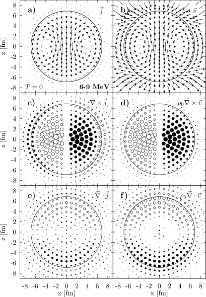
Figure 4: E1(T-0) current and velocity flow patterns (28)-(29) at x-z plane for the TM energy bin 6-9 MeV in ²⁰⁸Pb.:(a) nuclear current $\vec{j}$, (b) nuclear velocity $\vec{v}$, (c) current curl $\vec{\nabla}\times\vec{j}$, (d) velocity curl $\rho_{0}\vec{\nabla}\times\vec{v}$, e) current divergence $\vec{\nabla}\cdot\vec{j}$, and f) velocity divergence $\rho_{0}\vec{\nabla}\cdot\vec{v}$. In the panels (c)-(f), the flows, being perpendicular to the plane x-z, are exhibited by circles. The open (filled) circles represent flows along (opposite to) the y-axis. The flow magnitude is depicted by the size of the arrows and circles (in arbitrary units). The nuclear boarder is marked by a large circle. See explicit expressions for patterns in Appendix B.

IV.2 Flow patterns

As compared to the strength functions, the flow patterns deliver a more detailed information on nuclear dynamics. Here we depict not only nuclear current and velocity fields but also their divergences and curls. The patterns $\vec{\nabla}\cdot\vec{j}$ and $\vec{\nabla}\times\vec{j}$ are especially important since they directly indicate if the current contributes to CE. Obviously, only curl-free ($\vec{\nabla}\times\vec{j}$=0) currents are irrotational and coupled to CE. Instead, the divergence-free ($\vec{\nabla}\cdot\vec{j}$=0) currents carry the vorticity and are CE-unrestricted.

Note that the isovector GDR and isoscalar spurious c.m. motion are basically driven by the operator $rY_{1\mu}$ with the velocity field $\vec{v}\propto\vec{\nabla}(rY_{1\mu})$. They are the collective Tassie modes with $\vec{\nabla}\cdot\vec{j}=\vec{\nabla}\times\vec{j}=0$ and thus do not contribute to the curl and divergence patterns. Instead, the E1 TM and CM are characterized by the operators with $r^{3}$-dependence and so do not belong the Tassie modes. For them, the patterns $\vec{\nabla}\cdot\vec{j}$ and $\vec{\nabla}\times\vec{j}$ become indeed informative.

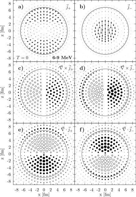
Figure 5: E1(T=0) flow patterns for the current components $\vec{j}_{+}$ (left) and $\vec{j}_{-}$ (right) at x-z plane for the TM energy bin 6-9 MeV in ²⁰⁸Pb. The current components $\vec{j}_{\pm}$ (a)-(b), as well as their curls (c)-(d) and divergences (e)-(f) are exhibited. Like in Fig. 4, the presentation is in terms of arrows and circles. See explicit expressions for the patterns in Appendix B.

In Fig. 4, different patterns for the energy bin 6-9 MeV containing the TM are considered. The panel (a) shows that, in accordance with our previous study Rep_PRC_13 , the current $\vec{j}$ is mainly of the toroidal nature (compare to Fig 1(a) for the schematic image of TM). The same takes place for the velocity field $\vec{v}$ exhibited in the panel (b). The velocity is not damped by the density factor and so is artificially strong at the nuclear surface (marked by the circle of the radius $R$ = 1.16 fm $A^{-1/3}$) and beyond. Following panels (c) and (e), the current curl is much stronger than its divergence, which confirms basically vortical character of the flow. The density-weighted curl and divergence of the velocity (panels (d)-(f)) are very similar to their current counterparts in the nuclear interior. A difference takes place only at the nuclear surface. So, up to the surface region, the HD vorticity determined by $\vec{\nabla}\times\vec{v}$ can be well characterized by $\vec{\nabla}\times\vec{j}$.

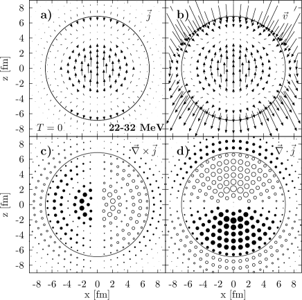
Figure 6: E1(T=0) flow patterns in ²⁰⁸Pb for the CM energy bin 22-32 MeV. See Fig. 4 for notation.

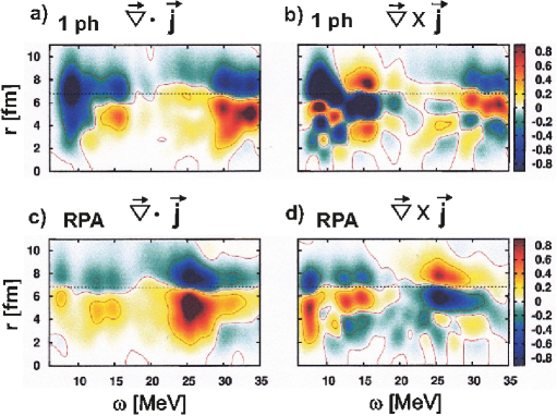
Figure 7: The coordinate-energy maps for the divergence (a,c) and curl (b,d) of the nuclear current in E1(T=0) channel in ²⁰⁸Pb. The upper (a,b) and lower (c,d) panels represent the 1ph and RPA strengths, respectively. The nuclear radius is marked by the dotted line. See explicit expressions for the patterns in Appendix B.

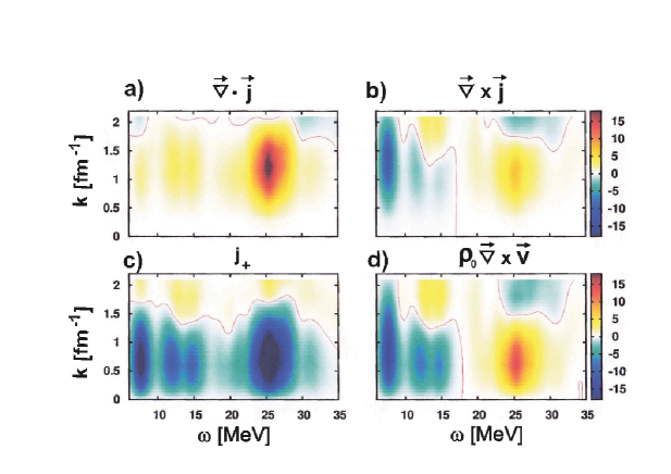
Figure 8: The E1(T=0) RPA formfactors (35) in ²⁰⁸Pb for divergence of current (a), curl of current (b), $j_{+}$ component of the current (c), density-weighted velocity curl (d). See explicit expressions for the patterns in Appendix B.

As shown in Sec. 2, the TM and CM operators are composed from $\vec{j}_{+}$ and $\vec{j}_{-}$ components of the nuclear current. Moreover, following Ra87 , the component $\vec{j}_{+}$ is treated as a measure of the nuclear vorticity. So it is worth to inspect the $\vec{j}_{+}$ and $\vec{j}_{-}$ flows in more detail. The relevant flow patterns are given in Fig. 5. It is seen (panels (a)-(b)) that $\vec{j}_{+}$ and $\vec{j}_{-}$ are essentially different: the former is maximal in the north and south poles while the later is maximal in the nuclear center. Despite this difference, curls of $\vec{j}_{+}$ and $\vec{j}_{-}$ are rather similar (panels (c)-(d)). The same takes place (up to the total sign) for the divergencies (panels (e)-(f)). Moreover, divergences and curls of $\vec{j}_{+}$ and $\vec{j}_{-}$ are of the same order of magnitude. So neither of these current components alone is suitable to represent neither vortical nor irrotational flows. Only their proper combinations, like TM and CM ones, may be appropriate for this aim. The value $\vec{j}_{+}$ has no any significant advantage over $\vec{j}_{-}$ as a measure of the vorticity, which makes the RW vorticity criterium Ra87 indeed questionable.

In Fig. 6, both fields $\vec{j}$ and $\vec{v}$ reproduce the typical compression dipole motion (compare to Fig 1(b) for the schematic image of CM). The divergence of the current is stronger than its curl. This is natural for CM which, being almost irrotational, is not, at the same time, the Tassie divergence-free mode.

IV.3 Coordinate-energy maps and form-factors

In Fig. 7, the smoothed coordinate-energy maps (30) for divergence and curl of the nuclear current are given for 1ph (unperturbed Hartree-Fock) and RPA E1(T=0) excitations. It is seen that both $\vec{\nabla}\cdot\vec{j}$ and $\vec{\nabla}\times\vec{j}$ are strong in a wide radial region 3 fm $<r<$ 10 fm around the nuclear surface at $\sim$ 7 fm. Following panels (a,b), the 1ph strength is concentrated in broad energy intervals: low-energy (LE) 4-17 MeV and high-energy (HE) 28-35 MeV. In both intervals, the curl and divergence are strong. The strength is multi-modal, which is common for non-collective (single-particle) excitations.

As seen from the panels (c,d) for the RPA case, inclusion of the residual interaction considerably changes the pictures. Being isoscalar, the residual interaction downshifts by energy both $\vec{\nabla}\cdot\vec{j}$ and $\vec{\nabla}\times\vec{j}$. In the CM region, the maxima are shifted from 30-35 MeV to 24-28 MeV. The RPA distributions correspond to the strength functions exhibited in Fig. 2 with the TM at $\sim$ 7 MeV, increased vorticity at 12-15 MeV and 25-30 MeV, and irrotational CM at $\sim$ 25 MeV.

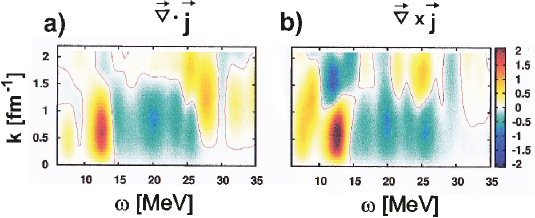
Figure 9: The E1(T=1) RPA formfactors (35) in ²⁰⁸Pb for divergence (a) and curl (b) of the current. See explicit expressions for the patterns in Appendix B.

It is remarkable that, after switch to RPA, both $\vec{\nabla}\cdot\vec{j}$ and $\vec{\nabla}\times\vec{j}$ become weaker in the GDR region 10-15 MeV. For the first glance, this result looks surprising. However both isovector GDR and isoscalar spurious c.m. motion are collective Tassie modes for which $\vec{\nabla}\cdot\vec{j}=\vec{\nabla}\times\vec{j}=0$. Then the panels (c)-(d) actually show the rest of $\vec{\nabla}\cdot\vec{j}$ and $\vec{\nabla}\times\vec{j}$ not yet washed out by the dominant Tassie collective dipole motion. So the Tassie motion can significantly suppress $\vec{\nabla}\cdot\vec{j}$ and $\vec{\nabla}\times\vec{j}$ initially produced by the single-particle motion. Instead, the CM and TM are not Tassie modes and thus survive in the RPA case. The plots (c,d) show that CM determined by $\vec{\nabla}\cdot\vec{j}$ (see Eq. (9)) is concentrated at $\sim$ 25 MeV while TM determined by $\vec{\nabla}\times\vec{j}$ (see Eq. (8)) is distinctive at $\sim$ 7 MeV. Some $\vec{\nabla}\times\vec{j}$ strength still remains at 12-15 MeV.

In Fig. 8, the smoothed E1(T=0) form-factors (35) for the values of interest are presented. Namely,the values $\vec{\nabla}\cdot\vec{j}$ , $\vec{\nabla}\times\vec{j}$, current component $j_{+}$, and $\rho_{0}\;\vec{\nabla}\times\vec{v}$, pertinent for CM,TM, RW, and HD strengths, are considered. Unlike the above transition coordinate-energy maps, the form-factors are direct constituents of $(e,e^{\prime})$ cross-section and their inspection may suggest the most optimal transfer momenta $k$ to observe a desirable mode. As follows from Fig. 9, the observation of $\vec{\nabla}\cdot\vec{j}$ and $\vec{\nabla}\times\vec{j}$, and thus related CM ($\sim$ 25 MeV) and TM ($\sim$ 7 MeV), requests rather large momenta, 0.8 fm${}^{-1}<k<$ 1.6 fm^-1, which testifies that CM and TM are mainly concentrated in the nuclear interior (which confirmed by Figs. 1, 4(a) and 7(a)). Instead the form-factors for $j_{+}$, and $\rho_{0}\vec{\nabla}\times\vec{v}$ are maximal for lower momenta, 0.6 fm${}^{-1}<k<$ 1.1 fm^-1, which points to their more surface character. Note that $j_{+}$ has strict maxima in both low-energy TM and high-energy CM regions. The form-factors for $\rho_{0}\vec{\nabla}\times\vec{v}$ and $\vec{\nabla}\times\vec{j}$ are similar, though the former is a bit stronger and shifted to lower $k$. The difference at low $k$ arises because these two form-factors are mainly distinguished by the coordinate dependence of the density $\rho_{0}(r)$, which is maximal at the nuclear surface (= low $k$).

For the comparison, in Fig. 9, the isovector E1(T=1) RPA form-factors for $\vec{\nabla}\cdot\vec{j}$ and $\vec{\nabla}\times\vec{j}$ are depicted. It is seen that they are weaker than in T=0 channel. The reason is again in the presence of the dominant collective Tassie mode. Indeed, within the Goldhaber-Teller model GT_48 , the GDR is essentially the Tassie mode. Hence we have the strong suppression of $\vec{\nabla}\cdot\vec{j}$ and $\vec{\nabla}\times\vec{j}$. Nevertheless, in Fig. 10, the GDR region still has noticeable $\vec{\nabla}\cdot\vec{j}$ and $\vec{\nabla}\times\vec{j}$ at 12-13 MeV. This could signal that the actual GDR is a combination of the Goldhaber-Teller GT_48 (Tassie mode) and Steinwedel-Jensen SJ_50 (beyond Tassie mode) flows. There are hints of the isovector TM at 11-13 MeV. The isovector CM is not seen. Perhaps it is shifted above the energy 35 MeV (as compared to the unperturbed 1ph CM strength at 29-35 MeV, depicted in Fig. 8(a)). Comparison of Figs. 9 and 10 shows that the T=0 channel is more suitable for the experimental search of TM and CM than the T=1 one.

V Discussion

The strength functions, flow patterns, coordinate-energy maps, and formfactors exhibited above show that $j_{+}$ component of the current has no any essential advantage over $j_{-}$ as the vorticity indicator. Indeed both components: i) are peaked in TM (basically vortical) and CM (basically irrotational) regions, ii) have curls and divergences of the same order of magnitude in TM region. This indicates that $j_{+}$ or $j_{-}$ alone cannot be a relevant measure of the vorticity. However, such a measure can be designed as a proper combination of $j_{+}$ or $j_{-}$. The toroidal mode is a natural case of such design. This transversal mode is free from the longitudinal part arising in the long-wave approximation (LWA) and its flow has a clear curl-like character.

As shown above, implementation of HD characteristics, like $\delta{\vec{v}}$, is not convenient because of their unphysical behavior at the nuclear surface and beyond. To demonstrate the HD vorticity, it is better to use the toroidal flow which gives a similar vorticity and is well behaved near the nuclear surface. Altogether, the numerical arguments favor TM as a measure of the vorticity.

Before discussing different aspects of nuclear vorticity, it is worth to define criteria for the vortical nuclear current. These could be: i) rotational flow pattern closely corresponding to the HD view, ii) decoupling from the CE i.e. transversal (divergence-free) character of the current. Such vortical nuclear current should correctly manifest itself in the basic test cases of TM and CM in E1(T=0) channel. Namely it has to dominate in the TM which is mainly vortical and vanish in the CM whose flow pattern is mainly irrotational.

The above requirement ii) is closely related to the definition of the independent current component (ICC) Ra87 ; Hei_82 which, together with electric longitudinal (reduced to the nuclear density) and magnetic transversal components, should constitute a complete set describing the charge and current distributions in the nucleus. There are at least two ways to define ICC.

The first way to determine ICC is proposed by Heisenberg Hei_82 and later Rawenthall and Wambach Ra87 . Here the decomposition of the nuclear current transition density

$$\delta\vec{j}(\vec{r})=-i\sum_{\lambda\mu}a_{\lambda\mu}\>(j_{\lambda\lambda-1}(r)\>\vec{Y}^{*}_{\lambda\lambda-1\mu}+j_{\lambda\lambda+1}(r)\>\vec{Y}^{*}_{\lambda\lambda+1\mu})$$ (36)

in terms of $j_{-}=j_{\lambda\lambda-1}(r)$ and $j_{+}=j_{\lambda\lambda+1}(r)$ is used. The component $j_{+}$ is claimed CE-unrestricted despite the CE (2) actually couples the radial parts of $\delta\rho_{\lambda}$, $j_{-}$, and $j_{+}$:

$$\omega\delta\rho_{\lambda}(r)= - \sqrt{\frac{\lambda}{2\lambda+1}}(\frac{d}{dr}-\frac{\lambda-1}{r})j_{\lambda\lambda-1}(r)$$ (37)

$$+ \sqrt{\frac{\lambda+1}{2\lambda+1}}(\frac{d}{dr}+\frac{\lambda+2}{r})j_{\lambda\lambda+1}(r)\;.$$

The claim is based on the analysis of the multipole moments given from the right and left sides of (37). The moments for $\delta\rho_{\lambda}$ and $j_{-}$ are coupled,

$$\omega\int drr^{\lambda+2}\delta\rho_{\lambda}(r)=\sqrt{\lambda(2\lambda+1)}\int drr^{\lambda+1}j_{\lambda\lambda-1}(r)\;,$$ (38)

while $j_{+}$-moments fully vanish. Therefore, $j_{+}$ is considered as CE-unrestricted and thus suitable to represent ICC and nuclear vorticity Ra87 . Following this prescription, vorticity of the nuclear current is fully determined by its $j_{+}$-component.

By our opinion, this prescription is not good at least for the following reasons. First, the vanishing of $j_{+}$-moments decouples $j_{+}$ from CE only in the integral sense while preserving the local coupling (37). In other words, $\vec{\nabla}\cdot\vec{j}_{+}(\vec{r})$ is not locally zero. Indeed in Fig. 5e) the field $\vec{\nabla}\cdot\vec{j}_{+}(\vec{r})$ is locally strong. However it has different sign at $z>0$ and $z<0$ and thus can vanish being integrated. Second, following (15), $j_{+}$ contributes to CM, which suggests a considerable vortical fraction in CM flow. At the same time, we know that CM is basically irrotational and has the gradient-like velocity Kva_PRC_11 . Third, our numerical analysis of TM/CM strengths and curl/divergences of the current does not reveal any essential advantage of $j_{+}$ over $j_{-}$ as the vorticity indicator. Altogether, the ansatz Ra87 to use $j_{+}$ as a measure of the vorticity and ICC looks doubtful.

Another (and more natural) way to define ICC has been proposed by Dubovik et al Dub_75_83 . Here the electric current transition density is decomposed into the longitudinal and transversal components,

$$\delta\vec{j}(\vec{r}) = \delta\vec{j}_{\parallel}(\vec{r})+\delta\vec{j}_{\perp}(\vec{r})\>,$$ (39)

$$\delta\vec{j}_{\parallel}(\vec{r}) = \vec{\nabla}\phi(\vec{r}),\quad\delta\vec{j}_{\perp}(\vec{r})=\vec{\nabla}\times\vec{\nabla}\times(\vec{r}\chi(\vec{r}))$$ (40)

where $\phi(\vec{r})$ and $\chi(\vec{r})$ are some scalar functions. As compared to the prescription Ra87 ; Hei_82 , this way looks more logical for the search of CE-unrestricted divergence-free ICC. Now we get $\delta\vec{j}_{\perp}$ as the natural ICC candidate from very beginning.

The current components can be expanded in the basis of eigenfunctions $\vec{\it J}^{(\kappa)}_{\lambda\mu k}({\vec{r}})$ ($\kappa$ = -, 0, +) of the vector Helmholtz equation (the similar expansion is familiar for the vector-potential, see e.g. EG_book ). Then the transversal component reads

$$\delta\vec{j}_{\perp}(\vec{r})=\sum_{\lambda\mu k}\vec{\it J}^{(+)}_{\lambda\mu k}({\vec{r}})\;m^{(+)}_{\lambda\mu}(k)$$ (41)

where $m^{(+)}_{\lambda\mu}(k)$ are electric transversal formfactors and integration by $k$ is assumed, In the LWA ($k\to 0$), the transversal component is reduced to the longitudinal one. After subtraction of the LWA part from $\delta\vec{j}_{\perp}$, we get at $k>0$ the toroidal current density. The transversal character of the toroidal current is also seen from (8) and (II.3). Being independent from $\delta\vec{j}_{\parallel}$ and thus decoupled from CE, the toroidal current can be considered both as ICC Dub_75_83 and relevant vortical part of the complete nuclear current. Unlike the prescription Ra87 ; Hei_82 , this vortical current is built from both $j_{+}$ and $j_{-}$ components, see e.g. (II.3). Its vorticity corresponds to HD one, see Sec. II C. Besides, the relevance of the TM current as a measure of the vorticity is confirmed by our numerical analysis of flow patterns. Altogether, our analysis shows that just TM and its current are best representatives of the nuclear vorticity.

Finally note that for more detailed study of the nuclear vorticity, it is desirable to go beyond RPA by taking into account the coupling to complex configurations, see e,g, the relevant extensions CoBo01 ; Sever_08 ; Li08 ; bianco12 ; Ry02 ; Sol92 . Note that, for the proper treatment of anharmonic effects, inclusion only of two-phonon configurations may not be enough. The impact of higher configurations and exact record of the Pauli principle are also necessary, see discussion Sol92 ; Ne90 . All these factors make anharmonic models very complicated. Anyway, before performing these involved investigations, a mere RPA exploration is desirable and this is just our case.

VI Conclusions

The problem of nuclear vorticity in isoscalar E1 excitations (toroidal and compression modes - TM and CM) was scrutinized within the Skyrme RPA with the force SLy6. A representative set of characteristics (strength functions, flow pattern for currents and velocities, curls and divergences of the current and its components, coordinate-energy maps and formactors) was inspected. Analysis of curls $\vec{\nabla}\cdot\vec{j}$ and divergences $\vec{\nabla}\times\vec{j}$ of the nuclear current, as direct indicators of the vortical/irrotational flow and coupling to the continuity equation (CE), was especially important. Note that the isovector GDR and isoscalar spurious c.m. motion, being the Tassie collective modes, do not contribute to $\vec{\nabla}\cdot\vec{j}$ and $\vec{\nabla}\times\vec{j}$. Instead, the TM and CM do not belong the Tassie modes and for them the curls and divergences become informative.

The numerical and analytical analysis shows that, unlike the prescription Ra87 ; Hei_82 , the nuclear vorticity is better described not by $j_{+}$ component of the nuclear current but by its transversal toroidal part Dub_75_83 composed from both $j_{+}$ and $j_{-}$ components. The toroidal motion is well decoupled from continuity equation, closely corresponds to the hydrodynamical picture of the vorticity, and provides a reasonable treatment of vortical/irrotational flow in toroidal and compression mods in E1(T=0) channel.

Appendix A Curls and divergencies

The curl and divergence of the current E1 transitions densities read:

$$\vec{\nabla}\times\delta\vec{j}^{\nu}_{1}(\vec{r})=i[rot\;j]^{\nu}(r)\;\vec{Y}^{*}_{11}$$ (42)

where

$$[rot\;j]^{\nu}(r)=\sqrt{\frac{2}{3}}\frac{d}{dr}j_{10}^{\nu}(r)+\sqrt{\frac{1}{3}}[\frac{d}{dr}+\frac{3}{r}]j_{12}^{\nu}(r)$$ (43)

and

$$\vec{\nabla}\cdot\delta\vec{j}^{\nu}_{1\mu}(\vec{r})=i[div\;j]^{\nu}(r)\;Y^{*}_{1}$$ (44)

where

$$[div\;j]^{\nu}(r)=\sqrt{\frac{1}{3}}\frac{d}{dr}j_{10}^{\nu}(r)-\sqrt{\frac{2}{3}}[\frac{d}{dr}+\frac{3}{r}]j_{12}^{\nu}(r)\;.$$ (45)

The velocity transition density can be decomposed like the current one (17):

$$\delta\vec{v}^{\nu}_{1\mu}(\vec{r})=[v_{10}^{\nu}(r)\vec{Y}^{*}_{10\mu}(\hat{\vec{r}})+v_{12}^{\nu}(r)\vec{Y}^{*}_{12\mu}(\hat{\vec{r}})]\;,$$ (46)

with

$$v_{10}^{\nu}(r)=\frac{j_{10}^{\nu}(r)}{\rho_{0}(r)}\;,\quad v_{11}^{\nu}(r)=\frac{j_{11}^{\nu}(r)}{\rho_{0}(r)}\;.$$ (47)

Then

$$\vec{\nabla}\times\delta\vec{v}^{\nu}_{1\mu}(\vec{r}) = i[rot\;v]^{\nu}(r)\;\vec{Y}^{*}_{11}\;,$$ (48)

$$\vec{\nabla}\cdot\delta\vec{v}^{\nu}_{1\mu}(\vec{r}) = [div\;v]^{\nu}(r)\;Y^{*}_{1}$$ (49)

with

$$[rot\;v]^{\nu}(r)=\sqrt{\frac{2}{3}}\frac{d}{dr}v_{10}^{\nu}(r)+\sqrt{\frac{1}{3}}[\frac{d}{dr}+\frac{3}{r}]v_{12}^{\nu}(r)\;,$$ (50)

$$[div\;v]^{\nu}(r)=\sqrt{\frac{1}{3}}\frac{d}{dr}v_{10}^{\nu}(r)-\sqrt{\frac{2}{3}}[\frac{d}{dr}+\frac{3}{r}]v_{12}^{\nu}(r)\;.$$ (51)

Appendix B Integral and average characteristics

The flows in Figs. 4-7 represent the integral vector variables (28) in $\{x,y=0,z\}$ cartesian plane, i.e. $\vec{A}(\vec{r})=A_{x}(x,y=0,z)\vec{e}_{x}+A_{z}(x,y=0,z)\vec{e}_{z}$. Namely, we use:

$$\vec{j}\to\vec{A}^{\nu}(\vec{r}) = \delta\vec{j}^{\nu}(\vec{r}),$$ (52)

$$\vec{j}_{10}\to\vec{A}^{\nu}(\vec{r}) = j_{10}^{\nu}(r)\vec{Y}^{*}_{10},$$ (53)

$$\vec{j}_{12}\to\vec{A}^{\nu}(\vec{r}) = j_{12}^{\nu}(r)\vec{Y}^{*}_{12},$$ (54)

$$\vec{\nabla}\times\vec{j}\to\vec{A}^{\nu}(\vec{r}) = [rot\;j]^{\nu}(r)\vec{Y}^{*}_{11},$$ (55)

$$\vec{\nabla}\times\vec{j}_{10}\to\vec{A}^{\nu}(\vec{r}) = \sqrt{\frac{2}{3}}\frac{d}{dr}j_{10}^{\nu}(r)\vec{Y}_{11},$$ (56)

$$\vec{\nabla}\times\vec{j}_{12}\to\vec{A}^{\nu}(\vec{r}) = \sqrt{\frac{1}{3}}[\frac{d}{dr}+\frac{3}{r}]j_{12}^{\nu}(r)\vec{Y}^{*}_{11},$$ (57)

$$\vec{v}\to\vec{A}^{\nu}(\vec{r}) = \delta\vec{v}^{\nu}(\vec{r}),$$ (58)

$$\rho_{0}(r)\vec{\nabla}\times\vec{v}\to\vec{A}^{\nu}(\vec{r}) = \rho_{0}(r)[rot\;v]^{\nu}(r)\vec{Y}^{*}_{11}.$$ (59)

The values in (52)-(54), (55)-(57), and (58,59) are taken from expressions (17), (42,43), and (46-48,50), respectively.

The scalar divergences in Figs. 4-7 use the values

$$\vec{\nabla}\cdot\vec{j}\to B^{\nu}(\vec{r}) = [div\;j]^{\nu}(r)Y^{*}_{1},$$ (60)

$$\vec{\nabla}\cdot\vec{j}_{10}\to B^{\nu}(\vec{r}) = \sqrt{\frac{1}{3}}\frac{d}{dr}j_{10}^{\nu}(r)Y^{*}_{1},$$ (61)

$$\vec{\nabla}\cdot\vec{j}_{12}\to B^{\nu}(\vec{r}) = -\sqrt{\frac{2}{3}}[\frac{d}{dr}+\frac{3}{r}]j_{12}^{\nu}(r)Y^{*}_{1},$$ (62)

$$\rho_{0}(r)\vec{\nabla}\cdot\vec{v}\to B^{\nu}(\vec{r}) = \rho_{0}(r)[div\;v]^{\nu}(r)Y^{*}_{1}$$ (63)

from expressions (44,45) and (49,47,51). The divergences are depicted in the figures as circles of the area proportional to $B(x,y=0,z)$. The filled (open) circles mean the positive (negative) sign of the variable.

Further, Figs. 8-10 give the average radial-energy maps (30) and form-factors (35) for the values

$$\vec{\nabla}\times\vec{j}\to C^{\nu}(r) = [rot\;j]^{\nu}(r)\;,$$ (64)

$$\vec{\nabla}\cdot\vec{j}\to C^{\nu}(r) = [div\;j]^{\nu}(r)\;,$$ (65)

taken from expressions (43) and (45).

References

- (1) A. Bohr and B. R. Mottelson, Nuclear Structure Vol. 2 (Benjamin, New York, 1974).
- (2) P. Ring and P. Schuck, Nuclear Many Body Problem, (Springer-Verlag N.Y.-Hedelberg-Berlin, 1980).
- (3) M.N. Harakeh and A. van der Woude, Giant Resonances (Clarendon Press, Oxford, 2001).
- (4) D.G. Raventhall, J. Wambach, Nucl. Phys. A475, 468 (1987).
- (5) V.M. Dubovik and A.A. Cheshkov, Sov. J. Part. Nucl. 5, 318 (1975); V.M. Dubovik and L.A. Tosunyan, ibid, 14, 504 (1983).
- (6) S.F. Semenko, Sov. J. Nucl. Phys. 34, 356 (1981).
- (7) G. Holzwarth and G. Ekart, Z. Phys. A283 219 (1977).
- (8) G. Holzwarth and G. Ekart, Nucl. Phys. A325, 1 (1979).
- (9) N. Paar, D. Vretenar, E. Khan, and G. Colo, Rep. Prog. Phys. 70, 691 (2007).
- (10) J. Kvasil, V.O. Nesterenko, W. Kleinig, P.-G. Reinhard, and P. Vesely, Phys. Rev. C84, 034303 (2011).
- (11) N. Ryezayeva et al, Phys. Rev. Lett. 89, 272502 (2002).
- (12) A. Repko, P.-G. Reinhard, V.O. Nesterenko, and J. Kvasil, Phys. Rev. C87, 024305 (2013).
- (13) F.E. Seer, T.S. Dumitrescu, T. Suzuki, C.H. Dasso, Nucl. Phys. A404, 359 (1983).
- (14) E.C. Caparelli and E.J.V. de Passos, J. Phys. G: Nucl. Part. Phys. 25, 537 (1999).
- (15) L.D. Landau and E. M. Lifshitz, Course of Theoretical Physics: Hydrodynamics Vol. 6, (Butterworth-Heinemann, Oxford, 1987).
- (16) J. Heisenberg, J. Lichtenstadt, C.N. Papanicolas, and J.S. McCarthy, Phys. Rev. C25, 2292 (1982).
- (17) M.N. Harakeh et al, Phys. Rev. Lett. 38, 676 (1977).
- (18) S. Stringari, Phys. Lett. B108, 232 (1982).
- (19) P.-G. Reinhard, Ann. Physik, 1, 632 (1992).
- (20) T.H.R. Skyrme, Phil. Mag. 1, 1043 (1956).
- (21) D. Vauterin, D.M. Brink, Phys. Rev. C5, 626 (1972).
- (22) Y.M. Engel, D.M. Brink, K. Goeke, S.J. Krieger, and D. Vauterin, Nucl. Phys. A249, 215 (1975).
- (23) M. Bender, P.-H. Heenen, and P.-G. Reinhard, Rev. Mod. Phys. 75, 121 (2003).
- (24) E. Chabanat, P. Bonche, P. Haensel, J. Meyer, and R. Schaeffer, Nucl. Phys. A635, 231 (1998).
- (25) W. Kleinig, V.O. Nesterenko, J. Kvasil, P.-G. Reinhard, and P. Vesely, Phys. Rev. C78, 044313 (2008).
- (26) V.O. Nesterenko, J. Kvasil, and P.-G. Reinhard, Phys. Rev. C66, 044307 (2002).
- (27) V.O. Nesterenko, W. Kleinig, J. Kvasil, P. Vesely, P.-G. Reinhard, and D.S. Dolci, Phys. Rev. C74, 064306 (2006).
- (28) A. Bohr and B. R. Mottelson, Nuclear Structure Vol. 1 (Benjamin, New York, 1969).
- (29) J. Kvasil, N. Lo Iudice, Ch. Stoyanov, and P. Alexa, J. Phys. G: Nucl. Part. Phys. 29, 753 (2003).
- (30) D.A. Varshalovich, A.N. Moskalev, V.K. Khersonskii, Quantum Theory of Angular Momentum (World Scientific, Singapore, 1976).
- (31) A.V. Varlamov, V.V. Varlamov, D.S. Rudenko, and M.E. Stepanov, Atlas of Giant Dipole Resonances, INDC(NDS)-394, 1999.
- (32) M. Uchida et al, Phys. Lett. B 557, 12 (2003).
- (33) M. Uchida et al, Phys. Rev. C 69, 051301(R) (2004).
- (34) D. Vretenar, A. Wandelt, and P. Ring, Phys. Lett. B487, 334 (2000).
- (35) D. Vretenar, N. Paar, P. Ring, and T. Niksic, Phys. Rev. C65, 021301(R) (2002).
- (36) G. Colo, N. Van Giai, P. Bortignon, and M.R. Quaglia, Phys.Lett. B485, 362 (2000).
- (37) M. Goldhaber and E. Teller, Phys. Rev. 74, 1046 (1948).
- (38) H. Steinwedel and J.H.D. Jensen, Z. Naturforsch. 5a, 413 (1950).
- (39) A. Carbone et al, Phys. Rev. C81, 041301(R) (2010).
- (40) J. Heisenberg, J. Lichtenstadt, C.N. Papanicolas, and J.S. McCarthy, Phys. Rev. C25, 2292 (1982).
- (41) J.M. Eisenberg and W. Greiner, Excitation Mechanisms of the Nucleus: Electromagnetic and weak interaction, (North-Holland, 1988).
- (42) G. Col and P. F. Bortignon, Nucl. Phys. A 696, 427 (2001).
- (43) A.P. Severyukhin, V.V. Voronov, N.V. Giai, Phys. Rev. C77, 024322 (2008).
- (44) E. Litvinova, P. Ring, and V. Tselyaev, Phys. Rev. C78, 014312 (2008).
- (45) D. Bianco,F. Knapp, N. Lo Iudice, F. Andreozzi, and A. Porrino Phys. Rev. C 85, 014313 (2012).
- (46) V. G. Soloviev, Theory of atomic nuclei : Quasiparticles and Phonons (Institute of Physics, Bristol, 1992).
- (47) V.O. Nesterenko, Z. Phys. A335, 147 (1990).