Spin Transfer Torque and Electric Current in Helical Edge States in Quantum Spin Hall Devices

Abstract

We study the dynamics of a quantum spin Hall edge coupled to a magnet with its own dynamics. Using spin transfer torque principles, we analyze the interplay between spin currents in the edge state and dynamics of the axis of the magnet, and draw parallels with circuit analogies. As a highlighting feature, we show that while coupling to a magnet typically renders the edge state insulating by opening a gap, in the presence of a small potential bias, spin-transfer torque can restore perfect conductance by transferring angular momentum to the magnet. In the presence of interactions within the edge state, we employ a Luttinger liquid treatment to show that the edge, when subject to a small voltage bias, tends to form a unique dynamic rotating spin wave state that naturally couples into the dynamics of the magnet. We briefly discuss realistic physical parameters and constraints for observing this interplay between quantum spin Hall and spin-transfer torque physics.

The study of symmetry protected topological insulators has led to a series of remarkable theoretical and experimental discoveriesHasan and Kane (2010); Hasan and Moore (2011); Maciejko et al. (2011). The initial prediction of the time-reversal invariant quantum spin Hall (QSH) insulatorKane and Mele (2005a, b) was soon realized in HgTe/CdTe quantum wellsBernevig et al. (2006); König et al. (2007) and, more recently, in InAs/GaSb quantum wellsLiu et al. (2008); Knez et al. (2011). One of the most exciting features of the quantum spin Hall insulator is the presence of robust, gapless edge states with counter propagating modes with opposite spin-polarization. The edge states form a so-called helical liquid which is a new class of 1D liquids that is perturbatively stable as long as time-reversal symmetry is preservedWu et al. (2006); Xu and Moore (2006). As predicted, experiments show that each edge, when biased, exhibits a quantized two-terminal, longitudinal conductivity of $e^{2}/h,$ even in the presence of disorder, as long as time-reversal symmetry is not brokenBernevig et al. (2006); König et al. (2007, 2008); Roth et al. (2009); Maciejko et al. (2011).

Some of the most interesting observable predictions concerning helical modes involve proximity coupling of the edge states to magnetic and/or superconducting layers that act to de-stabilize the edge and open a gapQi et al. (2008a, b); Fu and Kane (2008). For example, in the non-interacting limit, the helical liquid is simply a 1D Dirac fermion and it is well-known that the domain-walls of mass-inducing perturbations in this system lead to topological bound statesJackiw and Rebbi (1976); Su et al. (1979). These bound states can be the source of fractional charges, for the case of a magnetic domain wallJackiw and Rebbi (1976); Su et al. (1979); Qi et al. (2008a), or Majorana zero modes in a superconductor-magnet interfaceFu and Kane (2008). Our focus is on the coupling of magnetic perturbations to the helical liquid. Several works have discussed the coupling of dynamical magnets to the QSH edge states leading to various effects like adiabatic charge pumpingThouless (1983); Qi et al. (2008a), a spin-battery effectMahfouzi et al. (2010), and many related effects in 3D time-reversal invariant topological insulatorsGarate and Franz (2010); Yokoyama et al. (2010); Burkov and Hawthorn (2010); Mahfouzi et al. (2012); Ma et al. (2012); Chen et al. (2013).

In this article we consider the transport properties of a helical liquid in proximity to a dynamical ferromagnetic island and show that this coupled magnet-QSH edge system can exhibit a rich range of behavior due to spin-transfer torque physics. In the generic case, the magnetic island opens a gap and acts as a barrier for the helical liquid via the Zeeman coupling (if its magnetization has a component perpendicular to the spin-polarization of the helical liquid). Essentially the island provides a local mechanism for up-spin right-moving modes to backscatter to down-spin left-moving modes. This is a process that is usually strongly suppressed as it would require the electrons on one edge to scatter across the gapped interior of the sample to the opposite edge. Thus, in light of the gap formation, we would naively expect that if the edge is coupled to the magnetic island and then voltage biased, then as long as the voltage does not exceed the magnet-induced gap then there will be no longitudinal conductance on this edge. During this process we would expect charge to build up near the island until the potential counter-acts the applied voltage to reach a steady-state, i.e., we should have capacitor-like physics. In this article we show that, unexpectedly, once the magnet is dynamically influenced by a spin-transfer torque applied by the scattering edge states, then the edge can begin conducting current even at zero-temperature when the applied voltage is smaller than the magnet-induced gap. The resulting electrical behavior is then inductor-like.

The basic idea is as follows. A standard unbiased QSH bar carries gapless chiral edge currents of opposite spin (say polarized along $\hat{z}$ ) traveling in opposite directions, thus carrying zero charge current but two quantized units of spin current, if we ignore spin relaxation for now. The presence of a magnet, as in Fig. 1, couples the left and right movers and gaps these modes if the magnetization is not entirely along $\hat{z}.$ The gap renders the QSH edge a charge insulator, in that there is no initial charge current for a bias voltage with associated energy less than that of the magnet-induced gap. However, because of the spin-momentum locking, taking into account the spin degree of freedom yields more complex behavior. In the presence of such a bias the edge initially carries excess spin current on one side of the magnet. This imbalance of spin-current on the sides of the magnet provides a spin torque that results in the transfer of angular momentum and subsequent bias-controlled dynamics of the magnet. Again, because of the spin-momentum locking, the induced dynamics of the magnet in turn affects the QSH dynamics. For instance, in spite of the charge gap exceeding the applied voltage, the magnet induces a charge current in the edge as it rotatesQi et al. (2008a) due to the spin-transfer torque. Hence, we show that the magnet can act as an inductive circuit element instead of a capacitive element.

In what follows, we model the QSH-magnet coupled system and explore its dynamics employing spin-transfer torque methods. We analyze the approach to steady state, the nature thereof and characteristic relaxation times, and draw parallels with electrical circuit analogies. Applicable to experimental realizations, we estimate the effect from typical parameters of the QSH in HgTe/CdTe quantum wells and with the magnetic system of $K_{2}CuF_{4}$Yamada (1972). We then study the interplay between magnetization dynamics and bias voltage in the presence of interactions in the QSH edge states. Previously, within a Luttinger liquid framework, we have shown an instability towards an unusual spin-density wave orderingMeng et al. (2012a); here we find that the bias voltage endows this textured phase with unique dynamics.

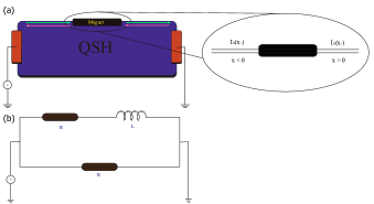
Figure 1: Quantum spin Hall insulator system coupled to a magnetic island on a single edge in the presence of a finite bias voltage. (a) We schematically illustrate the basic setup and zoom in the region of the island. (b) Circuit analogy for the Hall bar and magnet. Resistors represent the quantized $h/e^{2}$ resistance of each edge and the inductor represents the effect of the magnetic island.

Beginning with the free helical liquid, let us consider the QSH edge description which has the associated HamiltonianWu et al. (2006); Xu and Moore (2006)

$$H_{0} = \int dx\hbar v\left[\psi_{L\uparrow}^{\dagger}(x)(i\partial_{x})\psi_{L\uparrow}(x)-\psi_{R\downarrow}^{\dagger}(x)(i\partial_{x})\psi_{R\downarrow}(x)\right].$$

As shown in Fig. 2, these correspond to linearly dispersing edge states moving along the $x$-direction with speed $v,$ where the operator $\psi_{R\uparrow(L\downarrow)}$ annihilates an electron moving to the right(left) with up(down) spin. The proximity coupling between the magnet with magnetization $\overrightarrow{M}=(M_{x},M_{y},M_{z})$ and the QSH edge is given by the usual Zeeman coupling

$$H_{M}=-\mu_{0}\mu_{B}\overrightarrow{M}\cdot\overrightarrow{\sigma}$$ (2)

where $\mu_{0}$ is the the vacuum permeability, $\mu_{B}$ is the Bohr magneton and the Pauli matrices $\overrightarrow{\sigma}=(\sigma_{x},\sigma_{y},\sigma_{z})$ act on the space $\psi=[\psi_{R\uparrow}(x),\psi_{L\downarrow}(x)]^{T}$. In the region near the magnet, the QSH edge spectrum is effectively $\sqrt{(vp-\mu_{0}\mu_{B}M_{z})^{2}+(\mu_{0}\mu_{B})^{2}(M_{x}^{2}+M_{y}^{2})}$ which has an excitation gap induced by the magnet with magnitude $\Delta=2\mu_{0}\mu_{B}(M_{x}^{2}+M_{y}^{2})^{1/2}.$

Let us now consider the effect of a voltage bias $V$, which, for instance, we apply at the lead on the left in Fig. 1. Initially the spin currents in the left and right regions of the magnet are different, giving rise to a spin current imbalance $\Delta\overrightarrow{I}_{S}=[\overrightarrow{I}_{S}(x_{<})-\overrightarrow{I}_{S}(x_{>})]$, where $\overrightarrow{I}_{S}(x)=\frac{\hbar}{2}\psi^{\dagger}\frac{1}{2}(v\sigma_{z}\overrightarrow{\sigma}+\overrightarrow{\sigma}v\sigma_{z})\psi$, and $x_{<}(x_{>})$ is on the left (right) of the magnet as indicated in Fig. 1a. Because of the spin-momentum locking of the helical liquid, the spin current imbalance generically depends on the rotation frequency of the magnet. For simplicity, let us consider the case when the magnet rotates in-plane at a frequency ($\frac{\Omega_{M}}{2\pi}$). We can transform the full edge Hamiltonian $H=H_{0}+H_{M}$ to the rotating frame via the transformation $H^{\prime}=UHU^{\dagger}-iU\partial U^{\dagger}$, where $U=e^{i\frac{\Omega_{M}t}{2}\sigma_{z}}$Mahfouzi et al. (2010). In the new basis, the Hamiltonian takes the resultant form

$$H_{{\rm{rot}}}=\left[\begin{array}[]{cc}\hbar(-iv\partial_{x}-\frac{\Omega_{M}}{2})&-\mu_{0}\mu_{B}M_{s}\\ -\mu_{0}\mu_{B}M_{s}&\hbar(iv\partial_{x}+\frac{\Omega_{M}}{2})\end{array}\right],$$ (3)

where there is a rotation-induced voltage shift of $\hbar\Omega_{M}/e$ which is opposite for each spin component (see Fig. 2b). After imposing the appropriate boundary conditions and matching $\psi$ fields at the interfaces between the unperturbed helical liquid and the magnet, we find the initial spin current imbalance

$$\Delta\overrightarrow{I}_{S}(t=0)=\frac{eV-\hbar\Omega_{M}}{2\pi}\hat{z}.$$ (4)

Here have assumed that the length of magnet, $L_{M}$, is long enough , $L_{M}\gg\frac{\hbar v}{\mu_{0}\mu_{B}M_{s}}$, that a low-energy electron incident on the magnet barrier is completely reflected; accounting for tunneling requires a simple modification.

The spin-current imbalance applies a torque on the magnet and we can appeal to spin transfer torque (STT) physics to analyze the coupled dynamics between QSH edge currents and the magnet. Applying the well-established STT formalismSlonczewski (1996); Berger (1996), the dynamics is described by the Landau-Lifshitz equation

$$\gamma^{-1}\partial_{t}\overrightarrow{M}=-D\overrightarrow{M}\times M_{z}\hat{z}+\frac{1}{V_{M}}\hat{M}\times(\Delta\overrightarrow{I}_{S}\times\hat{M})$$ (5)

where $\gamma$ is the gyromagnetic ratio of the magnet, $V_{M}$ is the volume of the magnet, and $\hat{M}$ is the unit vector directed along the magnetization $\overrightarrow{M}$. The first term on the right-hand side accounts for the easy-plane anisotropy energy $\frac{1}{2}DM_{z}^{2}V_{M}$ of the magnet Bazaliy et al. (1998). The source of the anisotropy can be either intrinsic, as for an easy-plane magnet, or induced by the coupling to the edge states itself, though the latter effect is weak compared to usual magnetic energy scales. Thus we would generally desire the intrinsic anisotropy to be large to observe interesting dynamics since the edge coupling is usually small. The second term on the right-hand side accounts for the torque due to the spin current imbalance $\Delta\overrightarrow{I}_{S}$ derived above. Since the magnitude of the magnetization is effectively fixed, the spin torque along the direction of the magnetization has no effect; only the transverse part of this imbalanced spin current exerts the torque on the magnetization. We will see that the effect of this term is to drive the edge from an insulating state to a conducting state.

In general, the dynamics derived from substituting the spin imbalance expression of Eq. (4) into the dynamical equation of motion Eq. (5) has no simple solution. However, in most of the physical cases of interest we can make the approximation that the magnet always stays in-plane, i.e. $M_{z}\ll M_{S}$, where $M_{S}$ is the magnitude of the spontaneous magnetization. This condition holds for small enough bias voltages, i.e., bias voltages that are small compared to the magnet-induced gap, as will be justified in the proposed experimental setup to follow. With this approximation, we obtain the simple solution:

$$\Delta\overrightarrow{I}_{S} = \frac{eV}{2\pi}e^{-\frac{\gamma^{2}D\hbar}{2\pi V_{M}}t}\hat{z}$$

$$I_{C} = \frac{e^{2}V}{h}(1-e^{-\frac{\gamma^{2}D\hbar}{2\pi V_{M}}t})$$

$$M_{x}+iM_{y} = M_{S}e^{i\int_{0}^{t}\Omega_{M}dt^{\prime}}$$

$$M_{z} = \frac{2\pi}{e\gamma D}I_{C}$$ (6)

where $I_{C}=e\psi^{\dagger}v\sigma_{z}\psi$ is the charge current on the edge. Thus, we can immediately see that the dynamics involves a characteristic relaxation time $\tau=\frac{2\pi V_{M}}{\gamma^{2}D\hbar}$. The smaller the magnet and larger the anisotropy, the faster the relaxation.

We can simply illustrate the consequences of the dynamics. The STT on the magnet due to the spin current imbalance ($\Delta\overrightarrow{I}_{S}$) decays to zero, while the in-plane magnetization begins to rotate; the rotation frequency increases to the constant value $\frac{eV}{h}$ . Interestingly, in spite of the magnet-induced gap, the charge current ramps up to its quantized saturation value of $\frac{e^{2}}{h}V$, rendering the magnetic barrier transparent to charge. The spin transfer torque provides a magnetization along the $z$ direction, which reaches a new equilibrium value $\frac{eV}{\gamma D\hbar}$. In fact, this $z$ direction magnetization acts as an effective magnetic field causing the in-plane magnetization to precess. The charge current that flows here is essentially due to the same charge-pumping mechanism reported in Ref. Qi et al., 2008a for a rotating magnet. However, for our case the magnetization dynamics and the rotation frequency are intrinsically controlled by the applied bias voltage.

An even simpler picture for understanding the dynamics involves representing the geometry in Fig. 1a as an effective electrical circuit analog shown in Fig. 1b. The upper and lower QSH edges in Fig. 1 each provide a resistance of $R=\frac{h}{e^{2}}$. What our dynamical solution has shown is that the coupling of the edge states to the magnet can effectively be represented by an inductor with inductance $L=\tau R$. Hence, for this set up, charge is only transported through the lower edge initially, which yields an effective conductance of $e^{2}/h$. As with a real inductor, which stores energy in an induced field, here the energy is stored in the form of the anisotropy energy of the easy-plane magnet. Over time, the inductive component becomes transparent, allowing current to pass through. In the final steady state, the upper and lower edges both conduct perfectly and the conductance of the system rises and saturates to its quantized value of $2e^{2}/h.$

Let us briefly consider a physical magnetic system, for which we focus on $K_{2}CuF_{4}$, known for its large easy-plane anisotropyYamada (1972); Hirakawa and Yoshizawa (1979). This material possesses a spontaneous magnetization of $\mu_{0}M_{s}=0.124\text{T},\$ a gyromagnetic ratio $\gamma=-2\times 10^{11}\text{s}^{-1}\text{T }^{-1}$, and an out-of-plane anisotropy field $B_{A}=0.280\text{T}$, i.e. $D=\frac{B_{A}}{M_{s}}=2.26\mu_{0}$. For a typical magnet of volume $V_{M}=10^{4}\text{nm}\times 10^{2}\text{nm}\times 10^{2}\text{nm}$ these parameters provide a relaxation time estimate of $\tau=10^{-1}\text{s}.$ In order to be consistent with our approximation that $M_{z}\ll M_{S}$ ,we require an applied voltage to be smaller than $1\text{mV }$. This constraint confines the rotational frequency of the magnet ($\Omega_{M}=\frac{eV}{h}$) and the associated radiation to lie in the microwave range which indicates that microwave cavity resonator experiments may be useful for the observation of this effect.

While we have so far presented a clean, optimistic description of the effect, it must be mentioned that in addition to the primary contribution to the dynamics stemming from spin transfer torque, one also expects two sources of dissipation: (i) Gilbert damping of the magnetization dynamics and (ii) spin-relaxation of the helical liquid due to spin-orbit scattering. Gilbert damping contributes an additional term $\frac{\alpha}{M_{s}\gamma}\overrightarrow{M}\times\frac{d\overrightarrow{M}}{dt}$ to the right-hand side of Eq. (5) , where $\alpha$ is the damping constant. As shown in Appendix A we find that the damping provides an additional channel for relaxation, modifying the relaxation rate in Eq. (6) to $\tau^{-1}=\gamma^{2}D(\frac{\hbar}{2\pi V_{M}}+\alpha\frac{M_{S}}{|\gamma|})$. More importantly, it also changes the precession frequency to $\Omega_{M}=eV/(\hbar+\alpha 2\pi V_{M}M_{S}/|\gamma|)$. The effects of spin-orbit scattering will cause the spin carried by the helical liquid to relax as the charge current is carried from the leads to the magnetic island. This will reduce the amount of spin-current imbalance by a geometry and impurity-dependent factor $\zeta$ and subsequently the precession frequency will be reduced by the same factor. Both of these effects alter $\Omega_{M},$ and since the charge current is simply $e\Omega_{M},$ these two sources of dissipation will reduce the saturation conductance of the magnet-coupled edge from its quantized value. Notably, experiments indicate that spin-orbit scattering effects do not dominate the spin physics in HgTe/CdTe quantum wellsBrüne et al. (2012), however the Gilbert damping of the magnet will surely reduce the effective edge conductance, though hopefully not below an observable value.

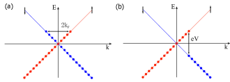
Figure 2: (a) Spectrum of the free helical liquid at finite chemical potential. With repulsive interactions present, system forms a gapped spin-density wave order parameter with wave vector $2k_{F}$, which nests the Fermi-points. (b) Spectrum of a free current-carrying helical liquid in the presence of a finite bias voltage. Alternatively, when coupled to a magnet,in the rotating frame of the magnet, the helical edges show a relative chemical potential shift. The magnetic order parameter that can effectively gap the associated Fermi-points has to thus connect states at different energies, exhibiting finite frequency dynamics.

So far we have neglected interactions within the QSH edges; we now examine the stability of the magnetization dynamics presented above in the presence of interactions. First we will consider the possibility of new interaction-driven phenomena, initially analyzing the QSH system in and of itself without the coupling to the magnet. As done previouslyWu et al. (2006); Xu and Moore (2006); Hou et al. (2009); Meng et al. (2012a, b), the interacting helical liquid can be explored within a Luttinger liquid framework through the bosonization of the fermion fields. We can use the boson fields $\phi$ and $\theta$ and the correspondence $\psi_{R\uparrow}(x)\sim e^{-i(\phi(x)-\theta(x))},\ \psi_{L\downarrow}(x)\sim e^{i(\phi(x)+\theta(x))}$ to bosonize the helical liquid. The Hamiltonian in Eq. (LABEL:eq:QSH-1), along with interactions, can be bosonized to yield the Luttinger liquid HamiltonianGiamarchi (2003)

$$H=\frac{1}{2\pi}\int dx\left[uK(\nabla\theta)^{2}+\frac{u}{K}(\nabla\phi)^{2}+2\mu\nabla\phi\right],$$ (7)

where $u=v((1+\frac{g_{4}}{2\pi v})^{2}-(\frac{g_{2}}{2\pi v})^{2})^{1/2}$ is the renormalized velocity, $K=(\frac{1+\frac{g_{4}}{2\pi v}-\frac{g_{2}}{2\pi v}}{1+\frac{g_{4}}{2\pi v}+\frac{g_{2}}{2\pi v}})^{1/2}\$ is the Luttinger parameter, and the $g_{2},g_{4}$ represent the standard interaction coupling constantsGiamarchi (2003). Values of $K<(>)1\$represent repulsive (attractive) interactions, and here we only consider repulsive interactions. We have also included a chemical potential ($\mu$) term to account for the edge Fermi-level not lying exactly at the Dirac point, a condition that leads to interesting physics in the presence of interactions (see Fig. 2a for an illustration in the free case). For repulsive interactions, the system is unstable to spontaneously breaking time-reversal symmetry and generating in-plane ferromagnetic order which opens a gap at the Fermi-energy when $\mu=0.$ If the chemical potential is not exactly tuned to be at the Dirac point, the system instead exhibits a spatial oscillation of the in-plane magnetic order, forming spin density wave (SDW) Giamarchi (2003); Meng et al. (2012a).

For the remainder of the calculations it is convenient to transform into the Lagrangian formulation, yielding the Lagrangian associated with Eq. 7

$$L_{\gamma}=\frac{1}{2\pi uK}((\partial_{t}\phi)^{2}-u^{2}(\nabla\phi)^{2}-2\mu uK\nabla\phi)+\partial_{t}(\gamma\phi).$$ (8)

Here the last term corresponds to a total derivative, which does not affect the classical equations of motion, but allows us to add a non-vanishing charge current. The parameter $\gamma$ represents an additional freedom that should be fixed by a physical quantity, which we choose to be the particle current operator $j$ given by

$$j=\left\langle\frac{\partial_{t}\phi}{\pi}\right\rangle,$$

thus fixing the choice: $\gamma=-j/Ku$.

The effect of repulsive interactions on the helical liquid can be seen by evaluating the appropriate susceptibilities. The primary quantity of interest is the susceptibility of the operator $O_{+}(x,t)\equiv\psi_{R\uparrow}^{\dagger}(x,t)\psi_{L\downarrow}(x,t)$ which is related to the in-plane magnetization of the edge state via $m_{+}(x,t)\equiv m_{x}(x,t)+im_{y}(x,t)=2\mu_{B}\langle O_{+}(x,t)\rangle$. To evaluate the spin susceptibility associated with the in-plane magnetization, $\chi_{m}(x,t)=-i\hbar\theta(t)\langle[O_{+}(x,t),O_{+}^{\dagger}(0,0)]\rangle$, it is easiest to first shift the $\phi$ field in the Lagrangian in Eq. (8) as $\tilde{\phi}(x,t)=\phi(x,t)+\mu Kx/u+\pi uK\gamma t$, and then employ standard Luttinger liquid techniques. As a function of temperature $T$ we find that the Fourier-transformed susceptibility in momentum and frequency space diverges as

$$\chi_{m}(\omega=-2\pi j,k=-2\tfrac{K}{u}\mu)\sim T^{2K-2}$$

near $(\omega_{c},k_{c})=(-2\pi j,-2K\mu/u).$

The divergence of the spin susceptibility is indicative of an intrinsic instability towards a magnetically ordered phase in the presence of repulsive interactions. As we discussed in previous work Meng et al. (2012a), the finite momentum at which the spin susceptibility diverges indicates that for $\mu\neq 0$ SDW order is preferred in which the in-plane magnetization spatially rotates over a length scale $\sim\frac{\pi u}{K\mu}$. A new effect is that, in the presence of an injected current, the susceptibility diverges at finite-frequency, i.e., the SDW order rotates at the frequency $2\pi j$ as a function of time. Thus, the edge can be carrying current and in a gapped, intrinsically-magnetized state if the SDW order rotates as a function of time.

We can heuristically illustrate why the time oscillation of the SDW occurs by resorting to the free-fermion description ($K=1$) where the current $j$ induced by a bias voltage $V$ can be determined by the filling of the single-particle energy spectrum as shown in Fig. 2b. In the presence of the repulsive interaction term $H_{int}=\psi_{R\uparrow}^{\dagger}\psi_{R\uparrow}\psi_{L\downarrow}^{\dagger}\psi_{L\downarrow}=O_{+}(x,t)O_{+}^{\dagger}(x,t)$ the system will try to develop in-plane magnetic order $\langle O_{+}(x,t)\rangle$, in order to induce a mass term $\psi_{R\uparrow}^{\dagger}\psi_{L\downarrow}\langle O_{+}^{\dagger}(x,t)\rangle$, that will open up a gap and lower the energy of the system. Notice that the most efficient way to lower the energy is to open up the gap at the Fermi points. When the current vanishes this implies that SDW order will form with a wave-vector that nests the two degenerate Fermi-points (see Fig. 2a). However, when there is finite current in this system, then, effectively, the two Fermi points are not at the same energy. In order to couple these two Fermi points that lie at different energies, the SDW has to have a time dependent part $\langle O_{+}(x,t)\rangle\sim e^{ieVt/\hbar}$ which is exactly why we observe a divergent spin susceptibility at finite frequency.

Finally, we revisit the coupling to the external magnet in the presence of interactions. Since the external magnetic island has been assumed to be uniform, we expect that to achieve the strongest coupling between QSH edge (with SDW order) and the external magnet, the length of the magnet should be smaller than the SDW wavelength $\sim\frac{\pi u}{K\mu}.$ The presence of a magnet, as in the non-interacting case, opens up a gap in the helical liquid. This is easy to see in the Luttinger liquid formalism, where the coupling between the edge state and external magnet in Eq.(2) has the Sine-Gordon form $\cos(2\phi-\theta_{H})$, where $\theta_{H}$ is the angle of the in-plane magnetization. This coupling is relevant in the renormalization group sense, and hence locks the phase $2\phi=\theta_{H}$ at low temperature. In previous work, we have analyzed the static effect of external magnets on the helical liquid at finite $\mu$ Meng et al. (2012a). For the dynamic situation we are considering in this work, one can derive the particle current as $j=\left\langle\frac{\partial_{t}\phi}{\pi}\right\rangle=\frac{\partial_{t}\theta_{H}}{2\pi}$ which is simply the adiabatic charge pumping on the QSH edge as derived in Ref. Goldstone and Wilczek (1981); Thouless (1983); Qi et al. (2008a), but now including interactions.

If the magnet is not initially rotating then, just as in the non-interacting case, we expect an initial spin current imbalance across the magnet when a voltage is applied. We can calculate this spin current imbalance, which, due to spin-momentum locking is proportional to the charge density difference across the the magnet, $\Delta I_{S}^{z}=\frac{\hbar}{2}v(\rho(x_{<})-\rho(x_{>}))=\frac{K}{2\pi}\frac{v}{u}eV$. Thus, even with interactions there is an initial spin-current imbalance which will apply a STT to the magnet. While a full analysis of the spin-transfer torque in the presence of interactions is beyond the scope of this work, we expect that just as with the non-interacting case, the excess spin current, now accompanied by an in-plane magnetization rotation of the edge, transfers angular momentum to the magnetic region. Once again, as with the non-interacting case, in steady state, a charge current will flow as the magnet evolves to a steady-state of rotation at a rate proportional to the applied voltage.

Applications - The unique combination of QSH physics and spin transfer torque gives rise to new ways of probing and manipulating the QSH edge, particularly by exploiting well-characterized magnetic materials and their information storage and access properties. i) Microwave resonator - We saw above that an excess QSH spin current produced by a voltage bias $V$ induces the magnet to precess at a frequency $eV/h$. This precession would result in microwave radiation of about $24\text{GHz}$ for typical bias voltages of order $0.1\text{meV}$. In principle, one can envision putting an array of QSH-coupled magnets in a microwave resonator to generate a voltage-tunable microwave laser. ii) Spin polarization detector- Thus far, we have assumed that the QSH spin axis coincides with that of the easy plane of the spin magnet. In principle, the two need not be aligned, effectively giving the excess QSH spin current components in the $xy$-plane and in turn affecting the dynamics of the magnet. Analyzing this dynamics would provide information on spin polarization in the QSH system. iii)AC QSH circuit - Information on the QSH edges can also be obtained by charge current measurements from the perspective of the circuit analogy of Fig. 1. The circuit description can be taken further by including a conventional capacitance element to produce oscillatory charge and spin currents. In conclusion, here we have presented an initial glimpse of the rich physics that can emerge through the interplay of QSH edge and spin-transfer torque physics.

Appendix A Gilbert damping

Now we include the Gilbert damping term in the spin transfer torque analysis of the Landau-Lifshitz-Gilbert equation:

$$\gamma^{-1}\partial_{t}\overrightarrow{M} = -D\overrightarrow{M}\times M_{z}\hat{z}+\frac{1}{V_{M}}\hat{M}\times(\Delta\overrightarrow{I}_{S}\times\hat{M})$$ (9)

$$+ \frac{\alpha}{M_{s}\gamma}\overrightarrow{M}\times\frac{d\overrightarrow{M}}{dt}$$

where the last term is due to Gilbert damping. Now we can write Eq. 9 in terms of components, and furthermore continue our approximation from the body of the text where we assume $M_{z}\ll M_{S}$ for total in-plane magnetization $M_{S}.$ Additionally, making an ansatz that $M_{x}=M_{S}\cos\theta(t),\ M_{y}=M_{S}\sin\theta(t),$

$$\gamma^{-1}\partial_{t}M_{z} = \frac{eV-\hbar\dot{\theta}(t)}{2\pi V_{M}}+\frac{\alpha}{\gamma}M_{S}\dot{\theta}(t)$$

$$\gamma^{-1}\partial_{t}M_{x} = -DM_{S}\sin\theta(t)M_{z}-\frac{\alpha}{\gamma}\dot{\theta}(t)\cos\theta(t)M_{z}$$

$$\gamma^{-1}\partial_{t}M_{y} = DM_{S}\cos\theta(t)M_{z}-\frac{\alpha}{\gamma}\dot{\theta}(t)\sin\theta(t)M_{z}.$$

In general the dynamics can be complicated, even after assuming $M_{z}\ll M_{S}.$ Let us consider our physical system of interest $K_{2}CuF_{4}$ where we estimate that $DM_{S}=0.28\text{T }.$ Thus for small voltages $V<1\text{mV }$, then $DM_{S}>-\frac{\alpha}{\gamma}\Omega_{M}$, as long as $\alpha<10^{-1}.$ With this approximation we have

$$\gamma^{-1}\partial_{t}M_{z} = \frac{eV-\hbar\dot{\theta}(t)}{2\pi V_{M}}+\frac{\alpha}{\gamma}M_{S}\dot{\theta}(t)$$

$$\gamma^{-1}\partial_{t}M_{x} = -DM_{S}\sin\theta(t)M_{z}$$

$$\gamma^{-1}\partial_{t}M_{y} = DM_{S}\cos\theta(t)M_{z}.$$

From here we see that Gilbert damping will just provide another channel for the damping of the imbalanced spin current, which will decrease relaxation time to

$$\tau=\left[\left(\frac{\hbar}{2\pi V_{M}}+\alpha\frac{M_{S}}{|\gamma|}\right)\gamma^{2}D\right]^{-1}$$ (10)

and decrease the rotation frequency to

$$\Omega_{M}=\frac{eV}{\hbar+\alpha 2\pi V_{M}M_{S}/\gamma}.$$ (11)

References

- Hasan and Kane (2010) M. Z. Hasan and C. L. Kane, Rev. Mod. Phys. 82, 3045 (2010).
- Hasan and Moore (2011) M. Z. Hasan and J. E. Moore, Annu. Rev. Condens. Matter Phys. 2, 55 (2011).
- Maciejko et al. (2011) J. Maciejko, T. L. Hughes, and S.-C. Zhang, Annu. Rev. Condens. Matter Phys. 2, 31 (2011).
- Kane and Mele (2005a) C. Kane and E. Mele, Phys. Rev. Lett. 95, 226801 (2005a).
- Kane and Mele (2005b) C. L. Kane and E. J. Mele, Phys. Rev. Lett. 95, 146802 (2005b).
- Bernevig et al. (2006) B. A. Bernevig, T. L. Hughes, and S.-C. Zhang, Science 314, 1757 (2006).
- König et al. (2007) M. König, S. Wiedmann, C. Brüne, A. Roth, H. Buhmann, L. W. Molenkamp, X.-L. Qi, and S.-C. Zhang, Science 318, 766 (2007).
- Liu et al. (2008) C. Liu, T. L. Hughes, X.-L. Qi, K. Wang, and S.-C. Zhang, Phys. Rev. Lett. 100, 236601 (2008).
- Knez et al. (2011) I. Knez, R.-R. Du, and G. Sullivan, Phys. Rev. Lett. 107, 136603 (2011).
- Wu et al. (2006) C. Wu, B. A. Bernevig, and S.-C. Zhang, Phys. Rev. Lett. 96, 106401 (2006).
- Xu and Moore (2006) C. Xu and J. E. Moore, Phys. Rev. B 73, 045322 (2006).
- König et al. (2008) M. König, H. Buhmann, L. W. Molenkamp, T. Hughes, C.-X. Liu, X.-L. Qi, and S.-C. Zhang, J Phys. Soc. Jpn. 77, 031007 (2008).
- Roth et al. (2009) A. Roth, C. Brüne, H. Buhmann, L. W. Molenkamp, J. Maciejko, X.-L. Qi, and S.-C. Zhang, Science 325, 294 (2009).
- Qi et al. (2008a) X.-L. Qi, T. L. Hughes, and S.-C. Zhang, Nat. Phys. 4, 273 (2008a).
- Qi et al. (2008b) X.-L. Qi, T. L. Hughes, and S.-C. Zhang, Phys. Rev. B 78, 195424 (2008b).
- Fu and Kane (2008) L. Fu and C. L. Kane, Phys. Rev. Lett. 100, 096407 (2008).
- Jackiw and Rebbi (1976) R. Jackiw and C. Rebbi, Phys. Rev. D 13, 3398 (1976).
- Su et al. (1979) W. Su, J. Schrieffer, and A. Heeger, Phys. Rev. Lett. 42, 1698 (1979).
- Thouless (1983) D. Thouless, Phys. Rev. B 27, 6083 (1983).
- Mahfouzi et al. (2010) F. Mahfouzi, B. K. Nikolić, S.-H. Chen, and C.-R. Chang, Phys. Rev. B 82, 195440 (2010).
- Garate and Franz (2010) I. Garate and M. Franz, Phys. Rev. Lett. 104, 146802 (2010).
- Yokoyama et al. (2010) T. Yokoyama, J. Zang, and N. Nagaosa, Phys. Rev. B 81, 241410 (2010).
- Burkov and Hawthorn (2010) A. Burkov and D. Hawthorn, Phys. Rev. Lett. 105, 066802 (2010).
- Mahfouzi et al. (2012) F. Mahfouzi, N. Nagaosa, and B. K. Nikolić, Phys. Rev. Lett. 109, 166602 (2012).
- Ma et al. (2012) M. Ma, M. Jalil, S. Tan, Y. Li, and Z. Siu, AIP Advances 2, 032162 (2012).
- Chen et al. (2013) J. Chen, M. B. A. Jalil, and S. G. Tan, arXiv preprint arXiv:1303.7031 (2013).
- Yamada (1972) I. Yamada, J Phys. Soc. Jpn. 33, 979 (1972).
- Meng et al. (2012a) Q. Meng, V. Shivamoggi, T. L. Hughes, M. J. Gilbert, and S. Vishveshwara, Phys. Rev. B 86, 165110 (2012a).
- Slonczewski (1996) J. C. Slonczewski, Journal of Magnetism and Magnetic Materials 159, L1 (1996).
- Berger (1996) L. Berger, Phys. Rev. B 54, 9353 (1996).
- Bazaliy et al. (1998) Y. B. Bazaliy, B. A. Jones, and S.-C. Zhang, Phys. Rev. B 57, R3213 (1998).
- Hirakawa and Yoshizawa (1979) K. Hirakawa and H. Yoshizawa, J Phys. Soc. Jpn. 47, 368 (1979).
- Brüne et al. (2012) C. Brüne, A. Roth, H. Buhmann, E. M. Hankiewicz, L. W. Molenkamp, J. Maciejko, X.-L. Qi, and S.-C. Zhang, Nat. Phys. 8, 485 (2012).
- Hou et al. (2009) C.-Y. Hou, E.-A. Kim, and C. Chamon, Phys. Rev. Lett. 102, 076602 (2009).
- Meng et al. (2012b) Q. Meng, S. Vishveshwara, and T. L. Hughes, Phys. Rev. Lett. 109, 176803 (2012b).
- Giamarchi (2003) T. Giamarchi, Quantum Physics in One Dimension (Oxford University Press, New York, 2003).
- Goldstone and Wilczek (1981) J. Goldstone and F. Wilczek, Phys. Rev. Lett. 47, 986 (1981).