Non-yrast spectra of odd-$A$ nuclei in a model of coherent quadrupole-octupole motion

Abstract

The model of coherent quadrupole and octupole motion (CQOM) is applied to describe non-yrast split parity-doublet spectra in odd-mass nuclei. The yrast levels are described as low-energy rotation-vibration modes coupled to the ground single-particle (s.p.) state, while the non-yrast parity-doublet structures are obtained as higher-energy rotation-vibration modes coupled to excited s.p. states. It is shown that the extended model scheme describes both the yrast and non-yrast quasi parity-doublet spectra and the related B(E1) and B(E2) transition rates in different regions of heavy odd-$A$ nuclei. The involvement of the reflection-asymmetric deformed shell model to describe the single-particle motion and the Coriolis interaction on a deeper level is discussed.

I Introduction

The observation of positive- and negative-parity states connected by E1 and E3 transitions in atomic nuclei is usually explained with the presence of quadrupole-octupole deformations EG87 ; BN96 . In the even-even nuclei one typically observes alternating-parity bands, whereas in odd-mass nuclei the spectrum is characterized by a quasi parity-doublet structure BN96 . The low-lying (yrast) structure of the quadrupole-octupole spectra was relatively well studied within different microscopic and collective model approaches Leand82 –Buck08 (see also BN96 and references therein). However, the interpretation and the model classification of the higher, non-yrast parts of these spectra is still limited.

Recently the model of Coherent Quadrupole-Octupole Motion (CQOM) b2b3mod ; b2b3odd was applied to describe non-yrast collective bands with positive and negative parities in even-even nuclei together with attendant B(E1), B(E2) and B(E3) transition probabilities MDSSL12 . It was shown that couples of $\beta$-bands and higher-energy (non-yrast) negative-parity bands can be interpreted within the model framework in the same way as the yrast alternating-parity bands. On this basis it was concluded that the octupole degrees of freedom have a persistent role at higher energies and the quadrupole-octupole structure of the spectrum develops towards the non-yrast region of collective excitations MDSSL12 .

The purpose of the present work is to examine the capability of the CQOM model scheme to describe non-yrast quadrupole-octupole excitations in odd-mass nuclei by extending the original consideration proposed in b2b3odd . For this reason it is assumed that some non-yrast level sequences with positive and negative parities observed in these nuclei can be associated to a higher-energy quasi parity-doublet structure of the spectrum. It is supposed that such a structure can appear as the manifestation of higher-energy quadrupole-octupole rotation-vibration modes coupled to the single-particle motion. The coupling of the odd nucleon to the even-even nuclear core as well as the Coriolis interaction are taken into account phenomenologically. At the same time the implemented approach is supposed to pave the way for a subsequent microscopic treatment of the odd-nucleon degrees of freedom. In this meaning the present work may be considered a necessary step towards a deeper understanding of the mechanism which governs the evolution of quadrupole-octupole dynamics in the higher-energy part of the spectrum in odd-mass nuclei.

This work is organized as follows. In Sec. II the CQOM model formalism for the split parity-doublet bands and its features in the non-yrast part of the spectrum are briefly presented. In Sec. III numerical results and a discussion on the application of the model to a number of odd-mass nuclei in the rare-earth and actinide regions are presented. In Sec. IV concluding remarks are given.

II Model of Coherent Quadrupole–Octupole Motion

The model Hamiltonian for odd-mass nuclei is taken as b2b3odd

$$H_{\mbox{\scriptsize qo}} = -\frac{\hbar^{2}}{2B_{2}}\frac{\partial^{2}}{\partial\beta_{2}^{2}}-\frac{\hbar^{2}}{2B_{3}}\frac{\partial^{2}}{\partial\beta_{3}^{2}}+U(\beta_{2},\beta_{3},I,K,\pi a),$$ (1)

where $\beta_{2}$ and $\beta_{3}$ are axial quadrupole and octupole deformation variables, respectively, and

$$U(\beta_{2},\beta_{3},I,K,\pi a)=\frac{1}{2}C_{2}{\beta_{2}}^{2}+\frac{1}{2}C_{3}{\beta_{3}}^{2}+\frac{X(I,K,\pi a)}{d_{2}\beta_{2}^{2}+d_{3}\beta_{3}^{2}}.$$ (2)

Here $B_{2}$ $(B_{3})$, $C_{2}$ $(C_{3})$ and $d_{2}$ ($d_{3}$) are quadrupole (octupole) mass, stiffness and inertia parameters, respectively. The quantity

$$X(I,K,\pi a) = \frac{1}{2}\biggl{[}d_{0}+I(I+1)-K^{2}$$ (3)

$$+ \left.\pi a\delta_{K,\frac{1}{2}}(-1)^{I+1/2}\left(I+\frac{1}{2}\right)\right]\ ,$$

involves the total angular momentum $I$, its third projection $K$ and the decoupling factor $a$ for the intrinsic states with $K=1/2$. The parameter $d_{0}$ determines the potential core at $I=0$. In the present work the decoupling factor is considered as a model parameter and is adjusted to the experimental data. In MDSS10 we show that a microscopically determined effect of the Coriolis interaction can be included in CQOM through an appropriate parity-projection particle-core coupling scheme in which the decoupling factor is calculated by using a reflection-asymmetric deformed shell model qocsmod .

Under the assumption of coherent quadrupole-octupole oscillations with a frequency

$$\omega=\sqrt{\frac{C_{2}}{B_{2}}}=\sqrt{\frac{C_{3}}{B_{3}}}\equiv\sqrt{\frac{C}{B}},$$ (4)

and after introducing ellipsoidal coordinates

$$\eta=\left[\frac{(d_{2}\beta_{2}^{2}+d_{3}\beta_{3}^{2})}{d}\right]^{\frac{1}{2}}\ \ \ \mbox{and}\ \ \ \phi=\arctan\left({\frac{\beta_{3}}{\beta_{2}}\sqrt{\frac{d_{3}}{d_{2}}}}\right)\ ,$$

such that

$$\beta_{2}=p\eta\cos\phi,\qquad\beta_{3}=q\eta\sin\phi,$$ (5)

with

$$p=\sqrt{\frac{d}{d_{2}}},\ \ \ q=\sqrt{\frac{d}{d_{3}}},\ \ \ d=\frac{1}{2}(d_{2}+d_{3}),$$ (6)

the collective energy of the system is obtained in the following analytic form b2b3odd

$$E_{nk}(I,K,\pi a) = \hbar\omega\left[2n+1+\sqrt{k^{2}+bX(I,K,\pi a)}\right],$$ (7)

$$n = 0,1,2,...\ ,\ \ k=1,2,3,...\ ,$$

where $n$ has the meaning of a radial $(\eta)$ quantum number, $k$ corresponds to an angular $(\phi)$ quantum number and $b=2B/(\hbar^{2}d)$ is considered as a parameter. The quadrupole-octupole vibration wave function is

$$\Phi^{\pi_{\mbox{\scriptsize c}}}_{nkI}(\eta,\phi)=\psi_{nk}^{I}(\eta)\varphi^{\pi_{\mbox{\scriptsize c}}}_{k}(\phi),$$ (8)

where the radial part

$$\psi^{I}_{nk}(\eta)=\sqrt{\frac{2c\Gamma(n+1)}{\Gamma(n+2s+1)}}e^{-c\eta^{2}/2}(c\eta^{2})^{s}L^{2s}_{n}(c\eta^{2})\$$ (9)

involves generalized Laguerre polynomials in the variable $\eta$ with $c=\sqrt{BC}/\hbar$ and $s=(1/2)\sqrt{k^{2}+bX(I,K,\pi a)}$. The angular part in the variable $\phi$ appears with a positive or negative parity, $\pi_{\mbox{\scriptsize c}}=(\pm)$, of the even-even core as follows

$$\varphi_{k}^{\pi_{\mbox{\scriptsize c}}=(+)}(\phi) = \sqrt{2/\pi}\cos(k\phi)\ ,\qquad k=1,3,5,...\ ,$$ (10)

$$\varphi_{k}^{\pi_{\mbox{\scriptsize c}}=(-)}(\phi) = \sqrt{2/\pi}\sin(k\phi)\ ,\qquad k=2,4,6,...\ .$$ (11)

The energy spectrum is determined in (7) by the quantum numbers $n$ and $k$. The parity-doublet structure is imposed by the condition $\pi=\pi_{\mbox{\scriptsize c}}\cdot\pi_{\mbox{\scriptsize sp}}$, where $\pi_{\mbox{\scriptsize sp}}$ is the parity of the odd-nucleon (single-particle) state. Then for a given state belonging to a parity-doublet the core parity is determined as $\pi_{\mbox{\scriptsize c}}=\pi\cdot\pi_{\mbox{\scriptsize sp}}$. The total core plus particle wave function for a state with an angular momentum $I^{\pi}$ belonging to a parity-doublet sequence in odd-even nuclei is given by b2b3odd

$$\Psi^{\pi,\pi_{\mbox{\scriptsize sp}}}_{nkIMK}(\eta,\phi) = \sqrt{\frac{2I+1}{16\pi^{2}}}\Phi^{\pi\cdot\pi_{\mbox{\scriptsize sp}}}_{nkI}(\eta,\phi)\left[D^{I}_{M\,K}(\theta)\mathcal{F}_{K}\right.$$ (12)

$$+ \left.\pi\cdot\pi_{\mbox{\scriptsize sp}}(-1)^{I+K}D^{I}_{M\,-K}(\theta)\mathcal{F}_{-K}\right]\ ,$$

where $D^{I}_{M\,K}(\theta)$ is the rotation Wigner function and $\mathcal{F}_{K}$ is the wave function of the odd-nucleon state.

In the present work it is supposed that the odd-nucleon parity $\pi_{\mbox{\scriptsize sp}}$ is a good quantum number, although in the more general treatment of the single-particle motion in the octupole deformed (reflection-asymmetric) mean-field (potential) the single nucleon state may appear with a mixed parity Leand82 -LC88 , MDSS10 . Then the parity-doublet is determined by a given $n$ and a pair of odd and even $k$-values, $k^{(\pi_{\mbox{\scriptsize c}}=+)}_{n}$ and $k^{(\pi_{\mbox{\scriptsize c}}=-)}_{n}$ ($k^{(+)}_{n}<k^{(-)}_{n}$), respectively. The $k$-values are determined so that $k=k^{(+)}_{n}$ for $I^{\pi=\pi_{\mbox{\scriptsize sp}}}$ and $k=k^{(-)}_{n}$ for $I^{\pi=-\pi_{\mbox{\scriptsize sp}}}$. The difference between $k^{(+)}_{n}$ and $k^{(-)}_{n}$ generates in (7) an energy splitting of the parity-doublet. That is why the term “quasi parity-doublet” was involved. According to the rule above the states having the same parity as the ground or bandhead state appear lower in energy and are characterized by the odd $k^{(+)}_{n}$ number, while the opposite-parity states are shifted up and are labeled by an even (and larger) $k^{(-)}_{n}$ number. The yrast doublet with $n=0$ is formed on the top of the ground state whose parity is $\pi_{\mbox{\scriptsize sp}}^{(n=0)}$. The non-yrast doublets with $n=1,2,...$ are coupled to excited s.p. or quasi-particle (q.p.) states (if the pairing correlations are taken into account) whose parities $\pi_{\mbox{\scriptsize sp}}^{(n)}$ determine the respective quasi-doublet structures according to the rule above. Also, the index $n$ labels the different intrinsic configurations to which the non-yrast doublets are coupled. The above model mechanism of the forming of parity-doublet structures takes into account the possibility for a switch, at certain higher angular momentum, of the s.p. state to which the doublet states are coupled to a state with an opposite parity, $\pi_{\mbox{\scriptsize sp}}\rightarrow-\pi_{\mbox{\scriptsize sp}}$. As suggested in b2b3odd the switch can be explained as the effect of an alignment process in the core JMS05 . In the present model this leads to a respective inversion of the parity $\pi_{\mbox{\scriptsize c}}$ of the vibration state at the given angular momentum and to a subsequent inversion of the mutual disposition of the parity-doublet counterparts, up-down $\leftrightarrow$ down-up. Such a situation is indeed observed in few cases and described by the model (see next section).

In the original application of the model to the yrast octupole spectra it was considered that for a given $n$ the nucleus always takes the lowest quadrupole-octupole vibration states with angular phonon numbers $k=1$ or $2$ depending on the parity b2b3mod ; b2b3odd . The generalization of the model description by including non-yrast alternating-parity spectra of even-even nuclei showed that a better agreement with the experimental data can be obtained if higher $k^{(\pm)}_{n}$-values are also allowed MDSSL12 . It was seen that the difference $\Delta k_{n}=k^{(-)}_{n}-k^{(+)}_{n}$ reasonably specifies the mutual disposition of the opposite-parity sequences in the spectrum. Therefore, it can be expected that the same meaning of the higher $k$-values will be valid for the parity-shift in the quasi-doublet bands of odd-mass nuclei. On the other hand, as recognized in MDSSL12 , in this case one has jumps of the quantum numbers $k_{n}^{(+)}$ and $k_{n}^{(-)}$ over several low-lying angular-phonon excitations within the set of levels characterized by given radial-phonon number $n$. Presently this is only justified by the meaning of $\Delta k_{n}$ as a characteristics of the mutual displacement of the opposite-parity sequences. The search for a deeper meaning and more sophisticated correlation between the quadrupole and octupole modes capable to compensate or explain these jumps is still an open issue. In this work we apply the original concept for the lowest $k^{(\pm)}_{n}=1$ or $2$ phonon numbers in the model description of yrast and non-yrast quasi parity-doublet spectra of odd-$A$ nuclei. At the same time in the end of the next section we discuss the difference between the obtained results and the result of calculations performed for the same nuclei by allowing higher $k_{n}^{(-)}$ values for the upper shifted doublet counterparts and fixed $k^{(+)}_{n}=1$ value for the counterparts whose parity coincides with the bandhead parity. For this reason we keep the formalism in its general form capable of treating unrestricted values of angular-phonon numbers.

By using the wave functions (12) one can calculate B(E$\lambda$) transition probabilities ($\lambda=1,2,3$) in the yrast and non-yrast quasi-doublet spectra. The relevant formalism was originally developed in b2b3mod ; b2b3odd and further extended to the non-yrast states of even-even nuclei MDSSL12 . In this work we apply the formalism developed in MDSSL12 . Due to the imposed axial symmetry the B(E$\lambda$) probabilities are non-zero only between states with the same $K$-values. Also, here the odd-nucleon wave function, $\mathcal{F}_{K}$ in (12), is not considered explicitly, while its parity is taken into account through the above explained parity-coupling scheme. As a result in this work we consider transition probabilities between states belonging to the same yrast or non-yrast quasi parity-doublet and, therefore, coupled to the same s.p. state (doublet bandhead). Then the CQOM reduced electric transition probabilities B($E\lambda$) with multipolarity $\lambda=1,2,3$ between the initial (i) and final (f) doublet states have the form

$$B(E\lambda;n_{i}k_{i}I_{i}K_{i}\rightarrow n_{f}k_{f}I_{f}K_{f})\hskip 108.12054pt$$

$$=\frac{2\lambda+1}{4\pi(4-3\delta_{\lambda,1})}\langle I_{i}K_{i}\lambda 0|I_{f}K_{f}\rangle^{2}R_{\lambda}^{2}(n_{i}k_{i}I_{i}\rightarrow n_{f}k_{f}I_{f}),$$ (13)

where $K_{i}=K_{f}$ corresponds to the same s.p. state. The factors $R_{\lambda}$ involve integrals over the radial $\eta$ and the angular $\phi$ variables and can be written in the following compact form

$$R_{\lambda}(n_{i}k_{i}I_{i}\rightarrow n_{f}k_{f}I_{f})\hskip 150.79968pt$$

$$=M_{\lambda}p^{a_{\lambda}}q^{b_{\lambda}}S_{l_{\lambda}}(n_{i}k_{i}I_{i};n_{f}k_{f}I_{f})I_{\lambda}^{\pi_{i},\pi_{f}}(k_{i},k_{f}),$$ (14)

with the exponents $a_{\lambda}=1,1,0$, $b_{\lambda}=1,0,1$ and indexes $l_{\lambda}=2,1,1$ for $\lambda=1,2,3$ , respectively. The integrals over $\eta$ are

$$S_{l}(n_{i}k_{i}I_{i};n_{f}k_{f}I_{f})\hskip 165.02606pt$$

$$=\int_{0}^{\infty}d\eta\psi_{n_{f}k_{f}}^{I_{f}}(\eta)\eta^{l+1}\psi_{n_{i}k_{i}}^{I_{i}}(\eta),\ \ \ l=1,2$$ (15)

while the integrals over $\phi$ read

$$I_{\lambda}^{\pi_{i},\pi_{f}}(k_{i},k_{f}) = \frac{2}{\pi}\int_{-\frac{\pi}{2}}^{\frac{\pi}{2}}A_{\lambda}(\phi)\varphi^{\pi_{f}\cdot\pi_{\mbox{\scriptsize sp}}}_{k_{f}}(\phi)\varphi^{\pi_{i}\cdot\pi_{\mbox{\scriptsize sp}}}_{k_{i}}(\phi)d\phi,\$$ (16)

where the factors $A_{\lambda}(\phi)$ represent series expansions defined in Eqs. (28)-(30) of MDSSL12 . Analytic expressions for the $\eta$-integrals (15) and explicit expressions for the $\phi$-integrals are given in Appendices B and C of MDSSL12 , respectively. The quantities $R_{\lambda}$ depend on the multipole charge factors $M_{\lambda}$, as determined in Eqs. (22) and (23) of MDSSL12 . The parameters $p$ and $q$ are defined in Eq. (6) above. However as shown in MDSSL12 they are not independent but one has $q=p/\sqrt{2p^{2}-1}$, so that only $p$ is kept as an adjustable parameter. Also, the integrals (15) depend on the parameter $c$ which enters the radial wave functions (9). In addition, an effective charge $e^{1}_{\mbox{\scriptsize eff}}$ is introduced to determine the correct scale of the B(E1) transition probabilities with respect to B(E2) MDSSL12 .

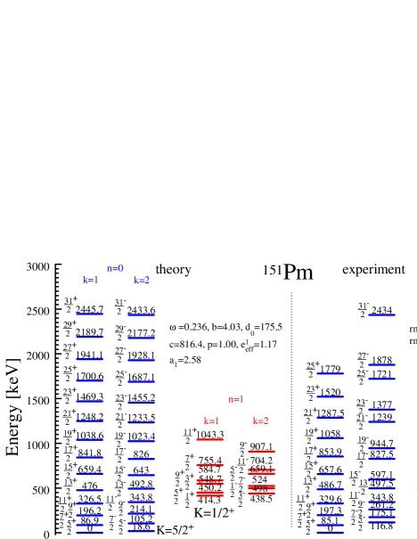
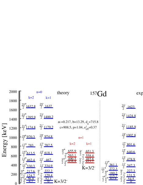
Figure 1: Theoretical and experimental quasi parity-doublet levels for ¹⁵¹Pm and ¹⁵⁷Gd. The root mean square (rms) deviations between the theoretical and experimental levels of the yrast band (rms₀), the first non-yrast band (rms₁) and the total rms factor for both bands (rms${}_{\mbox{\scriptsize total}}$) are given in keV. Data from ensdf . See the text for details.

The consideration of transition probabilities between states belonging to different parity-doublets, and with $K_{i}\neq K_{f}$, can be implemented after obtaining $\mathcal{F}_{K}$ within the reflection-asymmetric deformed shell model (DSM) qocsmod as done in MDSS10 and by taking into account the Coriolis $K$-mixing effect in the respective s.p. states as proposed in Mi13 . Such a task implies a natural connection of the collective CQOM model to an approach in which the ground state, the excited q.p. states, the respective decoupling factors (for $K=1/2$), as well as the Coriolis mixing contributions are obtained microscopically. Although the work in this direction is in an essential progress Mi13 , here we consider the s.p. degree of freedom phenomenologically. We consider that the knowledge of the pure collective CQOM description of quadrupole-octupole spectra, especially the yrast and non-yrast quasi-doublet levels, is a necessary step before attempting detailed implementation of the microscopic part of the approach. Thus for a given doublet we take the s.p. parity and the $K$-value as suggested by the experimental analysis or by microscopic calculations reported in the literature. The quasi-doublet band-heads are obtained as different rotation-vibration modes characterized by the CQOM oscillator quantum number $n=0,1,2,...$. In the cases of $K=1/2$ the decoupling factors $a_{n}$ for the respective doublets, labeled by $n$ and entering the expression (3), are adjusted according to the experimental data. It should be noted that these phenomenological decoupling factors are of special importance for determining the physically reasonable deformation regions where DSM calculations have to be performed after inserting the microscopic part in the CQOM. (See MDSS10 for more details on this consideration.)

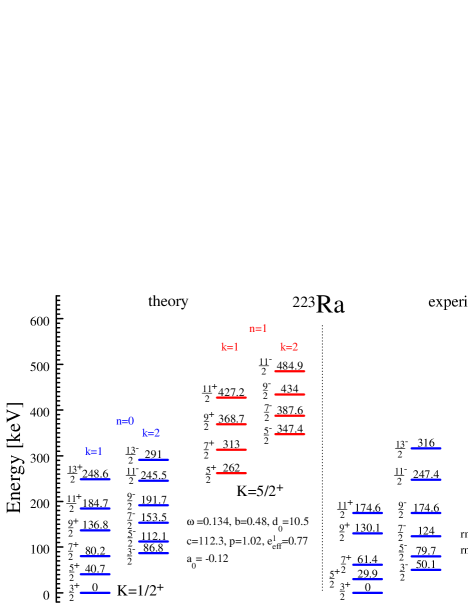
Figure 2: The same as Fig. 1, but for ²²³Ra.

III Numerical results and discussion

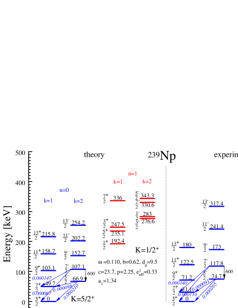
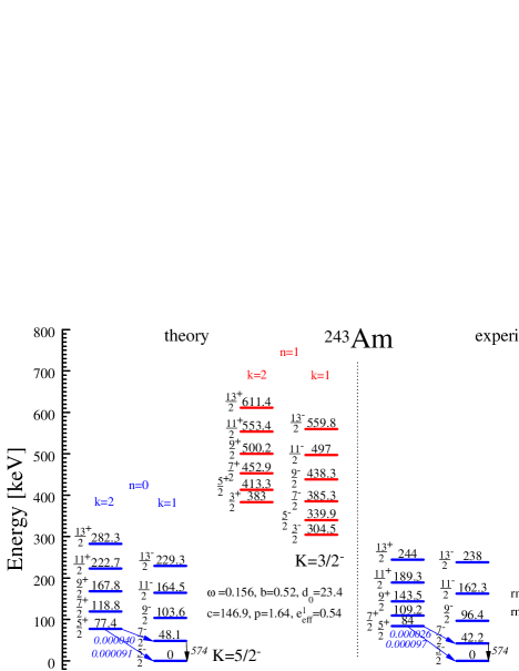
Figure 3: The same as Fig. 1, but for ²³⁹Np and ²⁴³Am. Theoretical and experimental B(E1) and B(E2) transition probabilities are also given (data from nudat2 ).

In this section results of the CQOM model calculations for several odd-mass nuclei are presented. The model energy levels are determined by Eq. (7) as

$$\tilde{E}_{nk}(I,K,\pi a)=E_{nk}(I,K,\pi a)-E_{0k_{0}}(I_{0},K_{0},\pi_{0}a_{0}),$$ (17)

where $I_{0}$, $K_{0}$, $k_{0}=1$, $\pi_{0}$ and $a_{0}$ correspond to the ground state. The model parameters $\omega$, $b$ and $d_{0}$ determine the energy levels, while the parameters $c$, $p$ and the effective charge $e^{1}_{\mbox{\scriptsize eff}}$ determine in addition the transition probabilities as explained below Eq. (16). These parameters are adjusted by simultaneously taking into account experimental data on the energy bands ensdf and the available B(E1) and B(E2) transition probabilities nudat2 . (Data on B(E3) probabilities are not available.) The theoretical B(E1) and B(E2) values are calculated through Eq. (13). In the case(s) of $K=1/2$ bandheads the decoupling factor(s) $a_{n}$ ($n=0$ for the yrast, and $n=1$ for the first non-yrast doublets) is (are) also adjusted. Calculations were performed for the nuclei ¹⁵¹Pm, ¹⁵⁷Gd, ²²³Ra, ²³⁹Np and ²⁴³Am. For each of them the yrast and one non-yrast quasi parity-doublet are considered together with a number of experimentally observed B(E1) and B(E2) transition probabilities.

The theoretical and experimental energy levels of the nuclei ¹⁵¹Pm, ¹⁵⁷Gd and ²²³Ra are compared in Figs. 1 and 2. In Fig. 3 both the energy levels and the transition probabilities for the nuclei ²³⁹Np and ²⁴³Am are given. The obtained parameter values are given in the figures. Also, the root mean square (rms) deviations between the theoretical and experimental levels of the yrast band (rms₀), the first non-yrast band (rms₁) and the total rms factors for both bands (rms${}_{\mbox{\scriptsize total}}$) are given in Figs. 1-3. The theoretical and experimental B(E1) and B(E2) transition probabilities for all considered nuclei are compared in Table 1. For each nucleus the model classification scheme accommodates one excited non-yrast quasi parity-doublet band. In all nuclei the theoretical energy sequences reproduce the structure of the experimentally observed yrast and non-yrast bands. This makes it meaningful to predict a few more states in some of the considered bands in order to show how the respective doublet-structures could develop with the angular momentum. More specifically, in Figs. 1-3 we add a number of predicted states to one of the parity-counterpart sequences in order to get an equal number of positive- and negative-parity levels in the theoretically obtained quasi-doublets.

The quasi-doublet sequences in the nuclei ¹⁵¹Pm and ¹⁵⁷Gd given in Fig. 1 have similar overall structures. In ¹⁵¹Pm we have a relatively well developed yrast doublet built on a $K=5/2^{+}$ ground state and a shorter non-yrast doublet considered to be coupled to a $K=1/2^{+}$ s.p. state. In the latter a strong Coriolis decoupling effect is observed, such that some higher-spin states appear at lower energy. This spin-interchange effect is partly reproduced in the model description through a relatively large decoupling-parameter value $a_{1}=2.58$. At the same time in the experimental yrast sequence we indicate an inversion of the up-down shift between the opposite-parity counterparts at $I^{\pi}=15/2^{\pm}$. This effect corresponds, according to the model assumption explained in the previous section, to an inversion of the s.p. parity and imposes an interchange of the $k^{(+)}_{0}=1$ and $k^{(-)}_{0}=2$ values in the model spectrum for $I^{\pi}\geq 15/2^{\pm}$. As a result the observed shift of the positive-parity states above their negative-parity counterparts is reproduced.

In ¹⁵⁷Gd both quasi-doublets are built on negative-parity s.p. states with $K=3/2^{-}$ which leads to the shift of the positive-parity counterparts in the lower part of the spectrum up in energy compared to the negative-parity ones. This is described according to the model scheme by assigning $k^{(-)}_{n}=2$ to the positive-parity states and $k^{(+)}_{n}=1$ ($n=0,1$) to the negative-parity ones. Similarly to ¹⁵¹Pm, in the yrast sequence of ¹⁵⁷Gd the two $k^{(\pm)}_{0}$ values are interchanged at $I^{\pi}=7/2^{\pm}$. We remark that for both nuclei in Fig. 1 the two $k$-values given above the theoretical yrast-band sequences correspond to the respective positive- or negative-parity counterparts before the interchange.

In ²²³Ra, given in Fig. 2, the yrast band is described by imposing $K=1/2^{+}$ instead of the experimentally suggested $K=3/2^{+}$. This is motivated by the previously indicated staggering behavior of the doublet splitting which is considered a manifestation of a Coriolis decoupling effect in that band b2b3odd . We remark that the decoupling factor obtains the same value $a_{0}=-0.12$ as in the model description obtained in b2b3odd for the yrast band only. (In Fig. 3(b) of b2b3odd this value was misprinted without the correct sign $(-)$.) The considered non-yrast quasi-doublet is built on a $K=5/2^{+}$ bandhead state. We see that the overall disposition of this doublet with respect to the yrast band is reasonably reproduced. The parity splitting in the yrast sequence is a bit overestimated by the theory, while that in the non-yrast band is slightly underestimated. Nevertheless, the root mean square (rms) deviations between the theoretical and experimental levels of the different bands as well as the total rms factor are obtained in quite reasonable limits between 20 and 25 keV (see Fig. 2).

The description of ²³⁹Np and ²⁴³Am given in Fig. 3 illustrates the applicability of the model scheme in the region of heavier nuclei. Here we can remark that the strong Coriolis effect in the non-yrast band of ²³⁹Np is adequately described with a decoupling factor $a_{1}=1.34$. As a result the situating of the $3/2^{-}$ state below the $1/2^{-}$ state and the $7/2^{-}$ state below the $5/2^{-}$ state in this band is well reproduced. At the same time the model predicts that in the positive-parity sequence of the non-yrast band the $5/2^{+}$ state will be placed below the $3/2^{+}$ state.

The theoretical values of the B(E1) and B(E2) transition probabilities, given in Table I, show an overall good agreement between theory and experiment. This makes it meaningful to predict a few more transition-probability values, especially between the lowest opposite-parity states in the non-yrast doublets (E1 transitions) as well as between states within sequences with the same parity (E2 transitions). Such predictions are given for all considered nuclei. It should be noted that data on transition probabilities in the non-yrast parts of the considered spectra are not available. In addition, we should remind that transitions between states belonging to different quasi parity-doublets are not included in the present consideration. For a number of yrast-band transitions larger discrepancies between theory and experiment are observed. In some cases, such as the E1 transitions in ²²³Ra, this can be explained with the more complicated structure due to the presence of the Coriolis interaction. However, we remark on the good model reproduction of the experimental B(E1) transition values in ¹⁵¹Pm, ²³⁹Np and ²⁴³Am. In the nuclei ²³⁹Np and ²⁴³Am for which only one B(E2) value is described we have an exact agreement between the theory and experiment due to the exact determination of the parameters $c$ and $p$ in the fitting procedure.

Table 1: Theoretical and experimental values of B(E1) and B(E2) transition probabilities in Weisskopf units (W.u.) for quasi parity-doublet spectra of several odd-mass nuclei. Notations: $I_{n_{i}}^{\pi_{i}}\rightarrow I_{n_{f}}^{\pi_{f}}$ with $n_{i}$ and $n_{f}$ denoting the doublet ($n=0,1$). The theoretical values are calculated in Eq. (13). The data are taken from nudat2 . The uncertainties (in parentheses) refer to the last significant digits in the experimental data.

Mult	Transition	Th [W.u.]	Exp [W.u.]
151Pm
E1	$5/2^{-}_{0}$ $\rightarrow$ $5/2^{+}_{0}$	0.0011	0.0014 (2)
E1	$7/2^{-}_{0}$ $\rightarrow$ $5/2^{+}_{0}$	$3.3\times 10^{-4}$	$>1.2\times 10^{-4}$
E1	$7/2^{-}_{0}$ $\rightarrow$ $7/2^{+}_{0}$	$6.3\times 10^{-4}$	$>2.1\times 10^{-4}$
E2	$7/2^{-}_{0}$ $\rightarrow$ $5/2^{-}_{0}$	8	$>8$
E2	$7/2^{+}_{0}$ $\rightarrow$ $5/2^{+}_{0}$	85
E1	$3/2^{-}_{1}$ $\rightarrow$ $1/2^{+}_{1}$	$6.3\times 10^{-4}$
E1	$5/2^{-}_{1}$ $\rightarrow$ $3/2^{+}_{1}$	$7.7\times 10^{-4}$
E2	$3/2^{+}_{1}$ $\rightarrow$ $1/2^{+}_{1}$	51
157Gd
E1	$5/2^{+}_{0}$ $\rightarrow$ $3/2^{-}_{0}$	$46.1\times 10^{-7}$	$4.6\times 10^{-7}$ (8)
E1	$5/2^{+}_{0}$ $\rightarrow$ $5/2^{-}_{0}$	$4.47\times 10^{-6}$	$10.3\times 10^{-6}$ (22)
E2	$5/2^{-}_{0}$ $\rightarrow$ $3/2^{-}_{0}$	311	293
E2	$7/2^{-}_{0}$ $\rightarrow$ $3/2^{-}_{0}$	130	119
E2	$7/2^{-}_{0}$ $\rightarrow$ $5/2^{-}_{0}$	195	230
E2	$7/2^{+}_{0}$ $\rightarrow$ $5/2^{+}_{0}$	18
E1	$5/2^{+}_{1}$ $\rightarrow$ $5/2^{-}_{1}$	$4.7\times 10^{-6}$
E1	$7/2^{+}_{1}$ $\rightarrow$ $5/2^{-}_{1}$	$6.6\times 10^{-6}$
E2	$5/2^{+}_{1}$ $\rightarrow$ $3/2^{+}_{1}$	30
E2	$7/2^{-}_{1}$ $\rightarrow$ $5/2^{-}_{1}$	199
223Ra
E1	$3/2^{-}_{0}$ $\rightarrow$ $3/2^{+}_{0}$	$4\times 10^{-5}$	$119\times 10^{-5}$ (16)
E1	$3/2^{-}_{0}$ $\rightarrow$ $5/2^{+}_{0}$	$4.2\times 10^{-4}$	$5.0\times 10^{-4}$ (9)
E1	$7/2^{-}_{0}$ $\rightarrow$ $5/2^{+}_{0}$	$3.30\times 10^{-4}$	$0.79\times 10^{-4}$ (24)
E1	$7/2^{-}_{0}$ $\rightarrow$ $7/2^{+}_{0}$	$1.4\times 10^{-5}$	$2.0\times 10^{-5}$ (22,-5)
E2	$7/2^{-}_{0}$ $\rightarrow$ $3/2^{-}_{0}$	17	10 (6)
E2	$7/2^{+}_{0}$ $\rightarrow$ $5/2^{+}_{0}$	18	70
E2	$7/2^{+}_{0}$ $\rightarrow$ $3/2^{+}_{0}$	148	44
E2	$11/2^{+}_{0}$ $\rightarrow$ $7/2^{+}_{0}$	210	280 (12)
E1	$5/2^{-}_{1}$ $\rightarrow$ $5/2^{+}_{1}$	$1.1\times 10^{-3}$
E1	$5/2^{-}_{1}$ $\rightarrow$ $7/2^{+}_{1}$	$4.9\times 10^{-4}$
E1	$7/2^{-}_{1}$ $\rightarrow$ $7/2^{+}_{1}$	$6.9\times 10^{-4}$
E2	$7/2^{+}_{1}$ $\rightarrow$ $5/2^{+}_{1}$	298
E2	$7/2^{-}_{1}$ $\rightarrow$ $5/2^{-}_{1}$	32
239Np
E1	$5/2^{-}_{0}$ $\rightarrow$ $5/2^{+}_{0}$	$2.10\times 10^{-4}$	$2.05\times 10^{-4}$ (11)
E1	$5/2^{-}_{0}$ $\rightarrow$ $7/2^{+}_{0}$	$9.8\times 10^{-5}$	$9.1\times 10^{-5}$ (4)
E1	$7/2^{-}_{0}$ $\rightarrow$ $5/2^{+}_{0}$	$7\times 10^{-5}$	$\geq 11\times 10^{-5}$
E1	$7/2^{-}_{0}$ $\rightarrow$ $7/2^{+}_{0}$	$1.5\times 10^{-4}$	$\geq 1.4\times 10^{-4}$
E2	$7/2^{-}_{0}$ $\rightarrow$ $5/2^{-}_{0}$	600	$\geq 600$
E2	$9/2^{-}_{0}$ $\rightarrow$ $7/2^{-}_{0}$	562
E1	$1/2^{-}_{1}$ $\rightarrow$ $1/2^{+}_{1}$	$2.1\times 10^{-4}$
E1	$3/2^{-}_{1}$ $\rightarrow$ $1/2^{+}_{1}$	$2.1\times 10^{-4}$
E2	$1/2^{-}_{1}$ $\rightarrow$ $3/2^{-}_{1}$	915
243Am
E1	$5/2^{+}_{0}$ $\rightarrow$ $5/2^{-}_{0}$	$9.1\times 10^{-5}$	$9.7\times 10^{-5}$(4)
E1	$5/2^{+}_{0}$ $\rightarrow$ $7/2^{-}_{0}$	$4\times 10^{-5}$	$2.6\times 10^{-5}$(3)
E2	$7/2^{-}_{0}$ $\rightarrow$ $5/2^{-}_{0}$	574	574 (9)
E2	$7/2^{+}_{0}$ $\rightarrow$ $5/2^{+}_{0}$	61
E1	$3/2^{+}_{1}$ $\rightarrow$ $3/2^{-}_{1}$	$1.7\times 10^{-4}$
E1	$3/2^{+}_{1}$ $\rightarrow$ $5/2^{-}_{1}$	$1.2\times 10^{-4}$
E1	$5/2^{+}_{1}$ $\rightarrow$ $5/2^{-}_{1}$	$7.7\times 10^{-5}$
E1	$7/2^{+}_{1}$ $\rightarrow$ $7/2^{-}_{1}$	$4.7\times 10^{-5}$
E2	$5/2^{-}_{1}$ $\rightarrow$ $3/2^{-}_{1}$	767
E2	$5/2^{+}_{1}$ $\rightarrow$ $3/2^{+}_{1}$	79

Here we can summarize that in all considered nuclei the rms deviations between the theory and experiment obtained for the different sequences as well as the total rms factors prove the good quality of the model description. We remark that the total rms factors do not exceed 50 keV, with the lowest rms${}_{\mbox{\scriptsize total}}$=23 keV being obtained for ²²³Ra and the higher one, 48 keV, observed in ¹⁵¹Pm. As mentioned in the previous section it can be expected that considerably better descriptions with lower rms factors may be expected if higher $k_{n}^{(-)}>2$ values are allowed for the upper quasi-doublet counterparts. We have performed such calculations for the same data in the same nuclei. For each nucleus the calculations were performed on a net over $k^{(-)}_{n}$ $(n=0,1)$ varying between $2$ and $20$ while $k^{(+)}_{n}$ was kept equal to 1. In this way the $k^{(-)}_{n}$ values which provide the best overall description of energy levels and transition probabilities were determined. As a result, essentially lower energy rms factors were obtained in: ²²³Ra with “favored” $k_{0}^{(-)}=4$ and $k_{1}^{(-)}=6$ values and rms${}_{\mbox{\scriptsize total}}$=7 keV; ²³⁹Np with $k_{0}^{(-)}=4$ and $k_{1}^{(-)}=2$ and rms${}_{\mbox{\scriptsize total}}$=15 keV; ²⁴³Am with $k_{0}^{(-)}=4$ and $k_{1}^{(-)}=6$ with rms${}_{\mbox{\scriptsize total}}$=18 keV. It is seen that in these nuclei the rms${}_{\mbox{\scriptsize total}}$ values obtained at $k_{n}^{(-)}>2$ are smaller than the values (given in Figs. 2 and 3) obtained for $k_{n}^{(-)}=2$ by a factor between 2 and 3. For the nuclei ¹⁵¹Pm with “favored” $k_{0}^{(-)}=6$ and $k_{1}^{(-)}=2$ values and rms${}_{\mbox{\scriptsize total}}$=37 keV, and ¹⁵⁷Gd with $k_{0}^{(-)}=2$ and $k_{1}^{(-)}=6$ and rms${}_{\mbox{\scriptsize total}}$=29 keV the improvement of the description is not too pronounced (see the rms values in Fig. 1).

The conclusion from the above mentioned calculations is that indeed the involvement of larger numbers of angular phonons leads to better model descriptions. Nevertheless the result illustrated in Figs. 1-3 shows that the imposing of the lowest quadrupole-octupole vibration modes with $k^{(+)}_{n}=1$ and $k^{(-)}_{n}=2$ still provides quite adequate interpretation and classification of the yrast and first non-yrast quasi-doublet energy sequences in the considered odd-mass nuclei. This means that the CQOM model is capable of reproducing the specific spectroscopic properties related to the simultaneous manifestation of quadrupole and octupole degrees of freedom in these nuclei. The use of the model with larger angular-phonon numbers can extend its applicability in wider regions of nuclei and quasi-doublet spectra, including higher non-yrast bands, but needs a detailed justification of the presence of lower model states for which experimental data are not observed. It should be noted that even on the present level of phenomenology, the CQOM model description provides a useful basis for further developments. As it was discussed in the end of Sec. II the knowledge of the decoupling factors as well as the model mechanism for the forming of parity-doublet spectra in odd-mass nuclei can guide the inclusion of microscopic calculations in the study.

IV Conclusion

In conclusion, the present work reports an application of the collective model of Coherent Quadrupole and Octupole Motion (CQOM) for the description of yrast and non-yrast quasi-doublet spectra in odd-mass nuclei. The calculations are performed by considering a zero number of radial quadrupole-octupole phonons in the yrast band and one radial-phonon excitation in the first non-yrast band. In both bands the lowest possible angular-phonon modes in the motion of the even-even core are considered. The results obtained for a number of odd-mass nuclei in the rare-earth and actinide regions illustrate the capability of the model to reproduce the structure of yrast and non-yrast energy levels together with the attendant B(E1) and B(E2) transition probabilities. The test of the model by allowing a higher number of angular phonons shows a better agreement with the experimental data, but still needs a justification of the jumps over the lower phonon numbers. At the same time the collective rotation-vibration structure of the spectra and the observed Coriolis decoupling effects are adequately taken into account. On this basis the present CQOM model descriptions can serve as a starting point for the application of a deeper collective and microscopic approach in the exploration of nuclear quadrupole-octupole collectivity. Work in this direction is in progress.

- (1) J. M. Eisenberg and W. Greiner, Nuclear Theory: Nuclear Models, 3rd ed. (North-Holland, Amsterdam, 1987), Vol. I.
- (2) P. A. Butler and W. Nazarewicz, Rev. Mod. Phys. 68, 349 (1996).
- (3) G. A. Leander, R. K. Sheline, P. Möller, P. Olanders, I. Ragnarsson, and A. J. Sierk, Nucl. Phys. A 388, 452 (1982).
- (4) G. A. Leander and R. K. Sheline, Nucl. Phys. A 413, 375 (1984).
- (5) G. A. Leander, Y. S. Chen, Phys. Rev. C 37, 2744 (1988).
- (6) A. Ya. Dzyublik and V. Yu. Denisov, Yad. Fiz. 56, 30 (1993) [Phys. At. Nucl. 56, 303 (1993)].
- (7) V. Yu. Denisov and A. Ya. Dzyublik, Nucl. Phys. A 589, 17 (1995).
- (8) N. V. Zamfir and D. Kusnezov, Phys. Rev. C 63, 054306 (2001).
- (9) N. Minkov, P. Yotov, S. Drenska, W. Scheid, D. Bonatsos, D. Lenis and D. Petrellis, Phys. Rev. C 73, 044315 (2006).
- (10) N. Minkov, S. Drenska, P. Yotov, S. Lalkovski, D. Bonatsos and W. Scheid, Phys. Rev. C 76, 034324 (2007).
- (11) P. G. Bizzeti and A. M. Bizzeti-Sona, Phys. Rev. C 77, 024320 (2008).
- (12) B. Buck, A. C. Merchant and S. M. Perez, J. Phys. G: Nucl. Part. Phys. 35, 085101 (2008).
- (13) N. Minkov, S. Drenska, M. Strecker, W. Scheid and H. Lenske, Phys. Rev. C 85, 034306 (2012).
- (14) N. Minkov, S. Drenska, M. Strecker and W. Scheid, J. Phys. G: Nucl. Part. Phys. 37, 025103 (2010).
- (15) S. Cwiok, J. Dudek, W. Nazarewicz, J. Skalski and T. Werner, Comp. Phys. Comm. 46, 379 (1987).
- (16) R. V. Jolos, N. Minkov and W. Scheid, Phys. Rev. C 72, 064312 (2005).
- (17) N. Minkov, Phys. Scripta T154, 014017 (2013).
- (18) http://www.nndc.bnl.gov/ensdf/.
- (19) http://www.nndc.bnl.gov/nudat2/indx_adopted.jsp.