A model selection approach for clustering a multinomial sequence with non-negative factorization

Abstract

We consider a problem of clustering a sequence of multinomial observations by way of a model selection criterion. We propose a form of a penalty term for the model selection procedure. Our approach subsumes both the conventional AIC and BIC criteria but also extends the conventional criteria in a way that it can be applicable also to a sequence of sparse multinomial observations, where even within a same cluster, the number of multinomial trials may be different for different observations. In addition, as a preliminary estimation step to maximum likelihood estimation, and more generally, to maximum $L_{q}$ estimation, we propose to use reduced rank projection in combination with non-negative factorization. We motivate our approach by showing that our model selection criterion and preliminary estimation step yield consistent estimates under simplifying assumptions. We also illustrate our approach through numerical experiments using real and simulated data.

1 Introduction

We consider a problem of clustering a sequence of multinomial observations. To be specific, consider a sequence $(X_{1},X_{2},\ldots,X_{T})$ of independent multinomial random vectors taking values in $\mathbb{N}^{d}$ for some $d\gg T$, where $\mathbb{N}=\{0,1,2,\ldots,\}$. For each $t=1,\ldots,T$, each $X_{t}$ is a multinomial random vector such that the number of trials is $N_{t}$ and the success probability vector is $P_{t}$. To simplify our notation, we write $X_{t}\sim{MN}(N_{t},P_{t})$. We allow the value of $N_{t}$ to depend on the value of $t$ and similarly, we allow the value of $P_{t}$ to depend on the value of $t$. Moreover, to formulate our clustering problem, we assume that there is a finite collection $\mathcal{Q}=\{Q_{1},Q_{2},\ldots,Q_{K}\}$ of $d$-dimensional probability vectors such that $\{P_{1},P_{2},\ldots,P_{T}\}=\mathcal{Q}$. Since $\{P_{1},P_{2},\ldots,P_{T}\}=\mathcal{Q}$, it follows that for each $k=1,\ldots,K$, there exists $t=1,\ldots,T$ such that $P_{t}=Q_{k}$. For each $t$, we let $\kappa(t)=k$ provided that $P_{t}=Q_{k}$, and to simplify our notation, we may also write $t\in k(\kappa)$ to mean $\kappa(t)=k$.

We assume that the value of $K$, $\kappa$ and $\mathcal{Q}$ are unknown, but the value of $(X_{1},\ldots,X_{T})$ is observed and forms the basis for statistical inference. Let $\theta=(\kappa,\mathcal{Q})$, and let $\Theta(K)$ be the set of all possible values for $\theta$. Note that $\kappa$ can be represented with an element in $\{1,\ldots,K\}^{T}$ and $\mathcal{Q}$ can be represented with an element in $[0,1]^{d\times K}$, i.e., a $d\times K$ non-negative matrix, where each column sums to $1$. Since the value of $K$ is assumed to be unknown, from a parameter estimation point of view, one also must consider the set $\Theta(K)$ for all $K=1,2,\ldots,T$ as a potential set to which the true parameter $\theta$ belongs. Then, we let

$$\Theta=\cup_{K=1}^{T}\Theta(K).$$ (1)

Henceforth, we write $K^{*}$ and $\theta^{*}=(\kappa^{*},\mathcal{Q}^{*})$ for the parameter that generates the data $(X_{1},X_{2},\ldots,X_{T})$. The estimates of $K$, $\kappa$ and $\mathcal{Q}$ are denoted by $\widehat{K}$, $\widehat{\kappa}$ and $\widehat{\mathcal{Q}}$ respectively, and we now use the letters $K$, $\kappa$, $\mathcal{Q}$ for a generic value that $\widehat{K},\widehat{\kappa},\widehat{\mathcal{Q}}$ can take respectively.

In this paper, we propose to take $\widehat{K}$, $\widehat{\kappa}$ and $\widehat{\mathcal{Q}}$ to be solutions to the optimization problems specified in (4) and (5). To this end, the rest of this paper is organized as follows.

In Section 2.1, we present the overall description of our approach, specifically introducing (4) and (5). In Section 2.2, we present a preliminary estimation technique, which can be used prior to performing a numerical search for the solution to (4). In Section 2.3, we specify the penalty term for our model selection criteria in (5).

In Section 3.1, we motivate our choice of the penalty term in (9) through Theorem 1 and 2. In Section 3.2, we motivate, in Theorem 3, our usage of the reduced rank projection step within our estimation steps.

In Section 4, we compare our model selection criterion with the conventional AIC via a Monte Carlo simulation experiment. We also study, through our approach, a two-sample test problem for comparing two graphs. This is done using simulated data sets, as well as a real data set involving the chemical and electrical connectivity structure of neurons of a C. elegan. Lastly, we apply our technique to a problem of determining the model dimension associated with the so-called Swimmer dataset which is well known to the non-negative factorization community (c.f. [1])

2 Background materials

2.1 General framework

To begin, we represent the sequence $(X_{1},X_{2},\ldots,X_{T})$ as an integer-valued random matrix $X$ so that the element in the $t$th column of $X$ is $X_{t}$. With slight abuse of notation, we denote the $i$th row and the $t$th column of $X$ by $X_{it}$. Since the sample value of $X$ is known, it follows that the sample values of $N_{1},N_{2},\ldots,N_{T}$ are known. Then, it follows that, denoting by $P$ the $d\times T$ matrix whose $t$th column is given by $P_{t}$, we have

$$\mathbf{E}_{\theta}[X\operatorname*{diag}(N_{1},\ldots,N_{T})^{-1}]=P,$$ (2)

where $\operatorname*{diag}(N_{1},\ldots,N_{T})$ is a $T\times T$ diagonal matrix such that its $t$th diagonal is $N_{t}$ and the expectation is taken with respect to the probability measure specified by $\theta$. Moreover, in general, it can be seen that $P$ can be factored as a product of two column stochastic non-negative matrices, namely, $W$ and $H$. Specifically,

$$P=WH,$$ (3)

where for each $k=1,\ldots,K$, the $k$th column $W_{k}$ of $W$ is $Q_{k}$ and for each $t=1,\ldots,T$, the $t$th column $H_{t}$ of $H$ is the basis vector of $\mathbb{R}^{K}$ such that its $k$-th entry is $1$ if and only if $\kappa(t)=k$.

In light of (2) and (3), when $X$ is observed without noise, i.e., $\mathbf{E}[X]=X$, and given that the value of $K$ is known, application of a non-negative factorization algorithm can recover $W$ and $H$ from $P$. However, in general, $X$ is random. Specifically, we have that for each $\theta\in\Theta$,

$$f_{X}(X_{1},X_{2},\ldots,X_{T}|\theta)=\prod_{t=1}^{T}\left({N_{t}\choose X_{t}}\prod_{i=1}^{d}P_{it}^{X_{it}}\right),$$

where for simplicity, we write

$${N_{t}\choose X_{t}}={N_{t}\choose X_{1t},X_{2t},\ldots,X_{dt}}.$$

Alternatively, we may also write, by grouping according to the value of $\kappa(t)$, that

$$f_{X}(X_{1},X_{2},\ldots,X_{T}|\theta)=\left(\prod_{k=1}^{K}\prod_{i=1}^{d}Q_{ik}^{\sum_{t\in k(\kappa)}X_{it}}\right)\prod_{t=1}^{T}{N_{t}\choose X_{t}}.$$

For simplicity, we may write

$$N=\sum_{t=1}^{T}N_{t}.$$

Then, for each $K=1,\ldots,T$, let $\widehat{\theta}(K)$ be an maximum $L_{q}$ estimate of $\theta^{*}$ with the restriction that the value of $\widehat{\theta}(K)$ must be an element of $\Theta(K)$, for some value of $q$ (c.f. [2]). Specifically, for each $K$ and $q$, we denote by $\widehat{\theta}(K;q)$, an maximum $L_{q}$ estimate of $\theta^{*}$ given $K$, and we have

$$\widehat{\theta}(K;q)\in\operatorname*{arg\,max}_{\theta\in\Theta(K)}\sum_{t=1}^{T}\sum_{i=1}^{d}X_{i}(t)\left(\frac{Q_{i,\kappa(t)}^{1-q}-1}{1-q}\right).$$ (4)

Note that by taking $q<1$ to $1$ in limit, then we see that

$$\lim_{q\rightarrow 1}\sum_{t=1}^{T}\sum_{i=1}^{d}X_{i}(t)\left(\frac{Q_{i,\kappa(t)}^{1-q}-1}{1-q}\right)$$

$$= \sum_{t=1}^{T}\sum_{i=1}^{d}X_{i}(t)\log(Q_{i,\kappa(t)}),$$

and as such, $\widehat{\theta}(K;1)$ reduces to a maximum likelihood estimate. When the value of $q$ is clear from context, we suppress $q$ from $\widehat{\theta}(K;q)$ and write $\widehat{\theta}(K)$ instead.

Then, we let $\widehat{K}$ be the smallest values of $K$ that minimizes the value of the following expression:

$$\Delta(K):=\sum_{t=1}^{T}D_{t}(X_{t},\widehat{Q}_{\widehat{\kappa}(t)})+\texttt{penalty}(K),$$ (5)

where $\texttt{penalty}(K)$ is assumed to be chosen a priori, $\widetilde{P}_{it}=X_{it}/N_{t}$, and

$$\quad D_{t}(X_{t},\widehat{Q}_{\widehat{\kappa}(t)}) :=D_{KL}({\widetilde{P}_{t}}||\widehat{Q}_{\widehat{\kappa}(t)})-\sum_{i=1}^{d}{\widetilde{P}_{it}}\log({\widetilde{P}_{it}})$$

$$=-\sum_{i=1}^{d}{\widetilde{P}_{it}}\log(\widehat{Q}_{i\widehat{\kappa}(t)}),$$

denoting by $D_{KL}(\mu_{1}||\mu_{2})$ the Kullback-Leibler divergence of $\mu_{2}$ from $\mu_{1}$. For reference, we let

$$D(\widehat{\mathcal{Q}},\widehat{\kappa}):=D(\widehat{\mathcal{Q}},\widehat{\kappa};X):=\sum_{t=1}^{T}D_{t}(X_{t},\widehat{Q}_{\widehat{\kappa}(t)}).$$

2.2 Preliminary estimation prior to $\operatorname*{MLqE}$

For our model selection problem, for each $K$, an estimator $\widehat{P}$ of $P^{*}$ as function of $\widetilde{P}$ must minimize the size $\|\widehat{P}-P^{*}\|$ of error while also allowing for non-negative factorization, i.e., $\widehat{P}=\widehat{W}\widehat{H}$ where $\widehat{W}$ and $\widehat{H}$ are $d\times K$ and $K\times T$ non-negative matrices. Directly computing an $\operatorname*{MLqE}$ to achieve this can be done numerically with varying degree of complexity, but in all cases, starting the search for $\operatorname*{MLqE}$ near $P^{*}=W^{*}H^{*}$ can be beneficial. To achieve this approximately for initializing our $\operatorname*{MLqE}$ search algorithm for numerical experiments, we propose a multi-step procedure in which $\operatorname*{OptSpace}$ and $\operatorname*{NMF}$ are used together. For more details on $\operatorname*{OptSpace}$ (and also on USVT, a related approach), we direct the reader to [3] (and [4]), and for $\operatorname*{NMF}$, to [5], [6] and [7].

Iteratively searching for a solution to the estimation problem in (4) can be computationally expensive. An approximate solution, which can be used as the initial point of the search, can be obtained in four steps, which are listed in Algorithm 1 collectively for convenience.

First we take a reduced rank projection of $X$ at the rank $K$. Specifically, we first compute the singular value decomposition of $X=U\Sigma V^{\top}$ with the diagonal of $\Sigma$ being sorted in a decreasing order, e.g. $\Sigma_{11}\geq\Sigma_{22}$. Then, we take

$$\widehat{X}=\operatorname*{OptSpace}(X;K):=\widehat{U}\widehat{\Sigma}\widehat{V}^{\top},$$ (6)

where $\widehat{\Sigma}$ is the upper $K\times K$ block of $\Sigma$, and $\widehat{U}$ and $\widehat{V}$ are the first $K$ columns of $U$ and $V$ respectively.

Because $\widehat{X}$ need not be non-negative, we then reset the negative entries of $\widehat{X}$ to zero. However, the resetting the negative entries of $\widehat{X}$ to zero can change the rank of $\widehat{X}$.

To correct this, after computing $\widehat{P}=\widehat{X}\operatorname{diag}(\bm{1}^{\top}\widehat{X})^{-1}$, we further perform non-negative factorization, which means we minimize $\|\widehat{P}-WH\|_{F}$ by running over all possible pairs of $d\times K$ matrix $W\geq 0$ and $K\times T$ matrix $H\geq 0$ (c.f. [5]).

In the last step, we define $\widehat{\kappa}$ by letting, for each $t=1,\ldots,T$, $\widehat{\kappa}(t)=k$ if and only if $\widehat{H}_{kt}\geq\widehat{H}_{k^{\prime}t}$ for all $k^{\prime}=1,\ldots,K$, where a tie, if any exists, is resolved by uniformly choosing among the tied indices. Then, estimate $\widehat{\mathcal{Q}}=\{\widehat{W}_{1},\ldots,\widehat{W}_{K}\}$.

The aforementioned steps for obtaining $\widehat{\kappa}$ and $\widehat{Q}$ are collectively denoted as $\operatorname*{MAP}(\widehat{W},\widehat{H})$ in the listing of Algorithm 1.

Upon obtaining the initial value of $(\widehat{Q},\widehat{\kappa})$, one can perform a numerical iterative search for $\operatorname*{MLqE}$, for example, using a variational method, an EM algorithm, an MCMC method, or a brute force iterative search. For an interested reader, in Section D, we outline an objective function to be maximized for an MCMC approach. In all cases, it is known that a good initialization of the chosen algorithm can improve its rate of convergence as well as allowing the algorithm to avoid a local stationary point. On the other hand, the number $K$ of clusters to be estimated still needs to be supplied, for each of these algorithms.

Algorithm 1 Preliminary Estimation prior to $\operatorname*{MLqE}$

1:$K=1,\ldots,T$ and data matrix $X$

2:procedure Preliminary Estimation

3:     $\widehat{X}\leftarrow\operatorname*{OptSpace}(X;K)$

4:     $\widehat{P}\leftarrow\widehat{X}\operatorname{diag}(\bm{1}^{\top}\widehat{X})^{-1}$

5:     $(\widehat{W},\widehat{H})\leftarrow\operatorname*{NMF}(\widehat{P};K)$

6:     $(\widehat{\kappa},\widehat{\mathcal{Q}})\leftarrow\operatorname*{MAP}(\widehat{W},\widehat{H})$

7:     return $(\widehat{\kappa},\widehat{\mathcal{Q}})$.

8:end procedure

2.3 Model selection criterion

For many application, the following standard model selection criteria are often used:

$$\Delta_{\operatorname*{AIC}}(K)=-\log(f_{X}(X|\widehat{\theta}(K)))+\texttt{penalty}_{\operatorname*{AIC}}(K),$$ (7)

$$\Delta_{\operatorname*{BIC}}(K)=-\log(f_{X}(X|\widehat{\theta}(K)))+\texttt{penalty}_{\operatorname*{BIC}}(K),$$ (8)

where

$\texttt{penalty}_{\operatorname*{AIC}}(K):=(d-1)K$, $\texttt{penalty}_{\operatorname*{BIC}}(K):=(d-1)K\log\left(N\right)$,

and $\widehat{\theta}(K)$ is chosen to be an MLE. Their derivation is based on analysis of an appropriate expected discrepancy (c.f. [8]) for a Gaussian regression model. In this section, we also follow this general approach, catering to our model.

Our model-based information criterion is obtained by appropriately penalizing the weighted log-likelihood of the multinomial model as specified in (5). Specifically, we consider, for each $s$ and $\gamma>0$,

$$\texttt{penalty}(K;s,\gamma):=\gamma\sum_{k=1}^{K}\frac{\widehat{Z}_{k}^{(K)}-1}{\left(\widehat{N}_{k}^{(K)}\right)^{s}},$$ (9)

where $\widehat{\kappa}^{(K)}$ is the estimate of $\kappa$ assuming that $K^{*}=K$, $\widehat{H}^{(K)}$ is the matrix such that $\widehat{H}^{(K)}_{kt}:=\bm{1}\{\widehat{\kappa}^{(K)}(t)=k\}$, $\widehat{N}_{k}^{(K)}:=\sum_{t=1}^{T}N_{t}\widehat{H}_{kt}^{(K)}$, $\widehat{Z}_{k}^{(K)}:=\sum_{i=1}^{d}\bm{1}\{\widehat{Q}^{(K)}_{ik}>0\}$. In words, $\widehat{N}_{k}^{(K)}$ is the number of “successes” from the $k$th cluster specified by $\widehat{\kappa}^{(K)}$. Also, $\widehat{Z}_{k}^{(K)}$ counts the number of non-zero entries from the $k$th cluster’s success probability vector $\widehat{Q}_{k}^{(K)}$, as specified by $\mathcal{\widehat{Q}}^{(K)}$.

We detail our motivation for (9) by way of Theorem 1 and 2. Intuitively, as $K$ increases, the term in (9) is expected to increase for a larger value of $K>K^{*}$ especially when $\widehat{W}_{i,c}^{(K)}>0$ and $\widehat{W}_{i,c^{\prime}}^{(K)}>0$ for $c\neq c^{\prime}$ for many values of $i$. In other words, when some columns of $\widehat{W}$ are “overly” similar to each other, the penalty term becomes more prominent (c.f. Table IV).

In Section E, we reduce (9) to $\Delta_{\operatorname*{AIC}}(K)$ and $\Delta_{\operatorname*{BIC}}(K)$ in (7) and (8) respectively, under some simplifying assumptions. However, for clustering a sequence of sparse multinomial data, the penalty terms in (7) and (8) that are appropriate for classical normal regression problems, can over-penalize, especially when the probability vectors $\mathcal{Q}$ contain many zeros (c.f. Figure 3).

3 Theoretical results

The main theoretical results of this paper are twofold. First, we motivate a particular choice of the form of the penalty term in (9) through an asymptotic analysis of $\Delta(K)$, under simplifying assumptions that $\widehat{\theta}(K^{*})=\theta^{*}\in\Theta(K^{*})$, $\widehat{\theta}(K^{*}-1)=\theta^{*,m}\in\Theta(K^{*}-1)$ and $\widehat{\theta}(K^{*}+1)=\theta^{*,s}\in\Theta(K^{*}+1)$. Following [9], we use the superscripted $m$ as a mnemonic for “merging”, and use the superscripted $s$ as a mnemonic for “splitting”. Second, we motivate the reduced rank projection approach for initializing the numerical search of the maximum $L_{q}$ likelihood estimate $\widehat{\theta}(K)\in\Theta(K)$.

3.1 Asymptotic derivation of the penalty term

In this section, we motivate a specific choice for the penalty term, $\texttt{penalty}(K)$, by computing the asymptotic form of the expected weighted discrepancy of $\Delta(K^{*})$ while taking the value of $\min_{t=1}^{T}\{N_{t}\}$ to $\infty$ along some sequence of index $\ell$. Let $\varphi(P):=-\sum_{t=1}^{T}\sum_{i=1}^{d}\frac{1}{N_{t}\overline{n}_{\kappa^{*}(t)}^{2}}\mathbf{E}\left[X_{i,t}\right]\log(P_{i,t}),$ where $P$ is associated with some $\theta\in\Theta$ through (2) and (3), the expectation is taken with respect to $\theta^{*}\in\Theta(K^{*})$, whence $P_{it}^{*}=\frac{1}{N_{t}}\mathbf{E}\left[X_{i,t}\right]$, and $\overline{n}_{k}=\sum_{t=1}^{T}\bm{1}\{\kappa^{*}(t)=k\}$.

Theorem 1.

Suppose that

1. for each $\ell$, we have $N_{1}^{(\ell)},\ldots,N_{T}^{(\ell)}$ such that for each $k=1,\ldots,K^{*}$, the number $N_{t}^{(\ell)}$ of trials is the same for all $t\in k(\kappa^{*})$,

2. for each $k=1,\ldots,K^{*}$, there exists $\overline{\lambda}_{k}\in(0,\infty)$ such that for each $t\in k(\kappa^{*})$

   $$\overline{\lambda}_{k}=\lim_{\ell}N_{t}^{(\ell)}/\ell.$$

Then,

$$\lim_{\ell\rightarrow\infty}\ell\left(\mathbf{E}[\varphi(\widehat{P})]-\varphi(P^{*})\right)=\frac{1}{2}\sum_{k=1}^{K^{*}}\frac{\overline{Z}_{k}^{*}-1}{\overline{n}_{k}\overline{\lambda}_{k}},$$

where $\widehat{P}=X^{(\ell)}\operatorname*{diag}(\bm{1}^{\top}X^{(\ell)})^{-1}$ and

$$\overline{Z}_{k}^{*}:=\overline{Z}_{k}^{*}(Q^{*}):=\sum_{i=1}^{d}\bm{1}\{W^{*}_{i,k}>0\}.$$ (10)

Theorem 1 suggests $(1,1/2)$ for the value of the pair $(s,\gamma)$ in (9). More importantly, we note that the non-zero entries do not contribute to the value of $\overline{Z}_{k}^{*}$ in (10).

For the rest of this section, we further study, through Theorem 2, the question of for what values of $s$ and $\gamma$, we can expect to see that $\widehat{K}$ chosen according to (5) with the penalty term specified by (9), estimate the true value $K^{*}$ with high probability.

Specifically, denoting by $N=\sum_{t}N_{t}$, in Theorem 2, we study the case in which choosing $(s,\gamma)=(1/2,\log(N))$ will lead to a model selection criterion that tends

(i)

not to under-estimate the value of $K^{*}$ when the alternative model is one that the $(K^{*}-1)$st and the $K^{*}$th clusters are “merged” into one,

(ii)

not to over-estimate the value of $K^{*}$, when the alternative model is one that for some $i$ and $j$, $\kappa^{*,s}(i)=K^{*}$ and $\kappa^{*,s}(j)=K^{*}+1$, i.e., the $K^{*}$th cluster is “split” into two.

Theorem 2.

Let $\theta^{*,m}=(\kappa^{*,m},\mathcal{Q}^{*,m})\in\Theta(K^{*}-1)$ and $\theta^{*,s}=(\kappa^{*,s},\mathcal{Q}^{*,s})\in\Theta(K^{*}+1)$, where we let

1. $\kappa^{*,m}:\{1,\ldots,n\}\rightarrow\{1,\ldots,K^{*}-1\}$ be such that $\kappa^{*,m}(i)=\kappa^{*}(i)$ for all $i$ that $\kappa^{*}(i)=k\leq K^{*}-2$ and $\kappa^{*,m}(i)=K^{*}-1$ for all $i$ that $\kappa^{*}(i)=K^{*}-1$ or $K^{*}$,

2. $\mathcal{Q}^{*,m}=\{Q^{*,m}_{k}\}_{k=1}^{K^{*}-1}$ be such that $Q^{*,m}_{k}=Q^{*}_{k}$ for $k=1,\ldots,K^{*}-2$ and $Q^{*,m}_{K^{*}-1}\in\mathbb{R}_{+}^{d}$ is a probability vector,

3. $\kappa^{*,s}:\{1,\ldots,n\}\rightarrow\{1,\ldots,K^{*}+1\}$ be such that $\kappa^{*,s}(i)=\kappa^{*}(i)$ for all $i$ that $\kappa^{*}(i)=k\leq K^{*}-1$ and $\kappa^{*,s}(i)\in\{K^{*},K^{*}+1\}$ for all $i$ that $\kappa^{*}(i)=K^{*}$, with $\kappa^{*,s}$ being surjective,

4. $\mathcal{Q}^{*,s}=\{Q^{*,s}_{k}\}_{k=1}^{K^{*}+1}$ be such that $Q^{*,s}_{k}=Q^{*}_{k}$ for $k=1,\ldots,K^{*}$ and then let $Q^{*,s}_{K^{*}+1}=Q^{*}_{K^{*}}$.

Suppose that $\lim_{N\rightarrow\infty}N_{t}/N>0$ for each $t=1,2,\ldots,T$, and that

$$D_{KL}(\theta^{*}||\theta^{*,m})\geq\min_{\theta\in\Theta(K^{*}-1)}D_{KL}(\theta^{*}||\theta)>0,$$ (11)

$$D_{KL}(\theta^{*}||\theta^{*,s})=\min_{\theta\in\Theta(K^{*}+1)}D_{KL}(\theta^{*}||\theta).$$ (12)

Then,

$$\lim_{N\rightarrow\infty}\mathbf{P}[\Delta^{*,m}(K^{*}-1)>\Delta^{*}(K^{*})]=1,$$ (13)

$$\lim_{N\rightarrow\infty}\mathbf{P}[\Delta^{*,s}(K^{*}+1)>\Delta^{*}(K^{*})]=1,$$ (14)

where

$$\Delta^{*}(K^{*}):=\sum_{t=1}^{T}D_{t}(X_{t},Q^{*}_{\kappa^{*}(t)})+\texttt{penalty}^{*}(K^{*}),$$

$$\Delta^{*,m}(K^{*}-1):=\sum_{t=1}^{T}D_{t}(X_{t},Q^{*,m}_{\kappa^{*,m}(t)})+\texttt{penalty}^{*,m}(K^{*}-1),$$

$$\Delta^{*,s}(K^{*}+1):=\sum_{t=1}^{T}D_{t}(X_{t},Q^{*,s}_{\kappa^{*,s}(t)})+\texttt{penalty}^{*,s}(K^{*}+1),$$

with

$$\texttt{penalty}^{*}(K^{*}):=\log(N)\sum_{k=1}^{K^{*}}\frac{\overline{Z}_{k}(Q^{*})-1}{(\sum_{t\in k(\kappa^{*})}N_{t})^{1/2}},$$

$$\texttt{penalty}^{*,m}(K^{*}-1):=\log(N)\sum_{k=1}^{K^{*}-1}\frac{\overline{Z}_{k}(Q^{*,m})-1}{(\sum_{t\in k(\kappa^{*,m})}N_{t})^{1/2}},$$

$$\texttt{penalty}^{*,s}(K^{*}+1)=\log(N)\sum_{k=1}^{K^{*}+1}\frac{\overline{Z}_{k}(Q^{*,s})-1}{(\sum_{t\in k(\kappa^{*,s})}N_{t})^{1/2}}.$$

In other words, in Theorem 2, assuming that $\widehat{\theta}(K^{*}-1)$ is such that its $\widehat{\mathcal{Q}}$ takes a form of $\{Q^{*,m}_{1},\ldots,Q^{*,m}_{K^{*}-1}\}$ and its $\widehat{\kappa}$ takes a form of $\kappa^{*,m}$, it follows that as $N\rightarrow\infty$, with high probability, $\Delta^{*,m}(K^{*}-1)>\Delta^{*}(K^{*})$, suggesting $\widehat{K}\geq K^{*}$. Similarly, in Theorem 2, assuming that $\widehat{\theta}(K^{*}+1)$ is such that its $\widehat{\mathcal{Q}}$ takes a form of $\{Q^{*,s}_{1},\ldots,Q^{*,s}_{K^{*}+1}\}$ and its $\widehat{\kappa}$ takes a form of $\kappa^{*,s}$, and that $\widehat{\theta}(K)=\theta^{*}$, it follows that as $N\rightarrow\infty$, with high probability, $\Delta^{*,s}(K^{*}+1)>\Delta^{*}(K^{*})$, suggesting $\widehat{K}\leq K^{*}$. Also, (5) with the penalty term specified by (9) with $(s,\gamma)=(1/2,\log(N))$ yields the specific form of $\Delta^{*}(K^{*})$, $\Delta^{*}(K^{*}-1)$ and $\Delta^{*}(K^{*}+1)$ in Theorem 2.

While proven under simplifying assumptions, through Theorem 1 and 2, we propose to choose the value of $(s,\gamma)$ to be $(1/2,\log(N))$ for consistence estimation of $K^{*}$.

On the other hand, as discussed in Section E, under some simplifying assumption, $(s,\gamma)=(1,1)$ can be associated with the conventional AIC, and similarly, $(s,\gamma)=(1/2,\log(N)/\sqrt{N/T})$ can be associated with the conventional BIC. For $(s,\gamma)=(1,1)$ and $(1/2,\log(N)/\sqrt{N/T})$, following the proof of Theorem 2, one can show results similar to (13) while the probability in (14) is positive but can be strictly less than $1$. For our numerical experiments in Section 4, to be comparable to the conventional AIC, we take $(s,\gamma)=(1,1)$ and we give a preference to a smaller value for $\widehat{K}$ if a near-tie occurs.

3.2 Reduced rank projection as a smoothing routine

The motivation behind using a reduced rank projection step is to remove random variation. As discussed in [3], when there is no missing entries in $X$, $\operatorname*{OptSpace}$ algorithm is equivalent to performing reduced-rank projection (or equivalently, singular value thresholding at a fixed rank). Specifically, it can be seen from [3, Theorem 4.4], that provided that a random matrix $M$ is assumed to be bounded appropriately and that its entries $\{M_{ij}\}$ are independent random variables, using $\operatorname*{OptSpace}$ yields a consistent estimate of $\mathbf{E}[M]$ under various conditions.

To give a more precise statement of our contribution on the topic, we begin by introducing some notation. Given a constant $C>0$, for each $i$ and $t$, let

$$Y_{i,t}:=X_{i,t}\wedge C:=\min\{X_{i,t},C\}.$$

Then, we let $\widehat{Y}$ be the result of a single iteration of the singular value threholding of $Y$ using the (true) value of $K^{*}$ of the matrix $\mathbf{E}[X]$. We will suppress, in our notation, the dependence of $X$, $Y$, and $\widehat{Y}$ on $C,n,T$ for simplicity.

Truncating each $X_{i}$ at $C$ yields an estimate that is biased due to truncation while its effect may diminish as the value of $C$ increases. We present an asymptotic result in which $C$ is allowed to grow as a function of $d$ and $T$ under several simplifying assumptions.

Our first simplifying assumption is that the mean matrix $\mathbf{E}[X]$ has a “finite” block structure, or equivalently, a “finite” checker-board type pattern. Specifically, we assume that $\mathcal{B}_{1},\ldots,\mathcal{B}_{B}$ partition the index set $\mathcal{B}:=\{(i,t):i=1,\ldots,d,t=1,\ldots,T\}$, where the value of $B$ is constant and does not depend on $C$, $d$ and $T$, Next, we assume also that for each $b=1,\ldots,B$, there exists a pair $(\nu_{b},p_{b})\in(0,\infty)\times(0,1)$ such that for each $(i,t)\in\mathcal{B}_{b}$, $\mathbf{E}[X_{i,t}]=\nu_{b}$ and $\lim_{d\wedge T\rightarrow\infty}|\mathcal{B}_{b}|/|\mathcal{B}|=p_{b}$. We assume that the values of $\{(\nu_{b},p_{b}):b=1,\ldots,B\}$ are constant and do not depend on $C$, $d$ and $T$.

We suppress in our notation, the dependence of $\nu_{b}$, $\mathcal{B}_{b}$, $\mathcal{B}$ and $C$ on $d$ and $T$ for simplicity. Also, $d\wedge T\rightarrow\infty$ means that the pair $(d,T)$ is indexed by $\ell=1,2,\ldots$, so that $\lim_{\ell\rightarrow\infty}\min(d_{\ell},T_{\ell})=\infty$.

Theorem 3.

Suppose that $N_{1},N_{2},\ldots,N_{T}$ are independent Poisson random variables, and that the rank of $\mathbf{E}[X]$ is $K^{*}$.

If $\lim_{T\wedge d\rightarrow\infty}C_{d,T}=\infty$ and $C:=C_{d,T}=o((d/T^{3})^{1/4})\wedge o(\log(T)^{1/2}/T)$,

then

$$\lim_{T\wedge d\rightarrow\infty}\operatorname*{MSE}(\widehat{Y};X)=0,$$

where $\operatorname*{MSE}(\widehat{Y};X):=\mathbf{E}\left[\frac{1}{dT}\|\widehat{Y}-\mathbf{E}[X]\|_{F}^{2}\right]$.

Note that generally, the rank of $\mathbf{E}[X]\leq K^{*}$ and for some cases, it is also possible to have the rank of $\mathbf{E}[X]<K^{*}$. In Theorem 3, to simplify our analysis, we have assumed that the rank of $\mathbf{E}[X]$ is $K^{*}$. Next, to consider Theorem 3 with respect to [3, Theorem 4.4], we note that the result in [3, Theorem 4.4] applies when the errors are independent while the entries of $\widehat{P}$ are correlated. Specifically, as a corollary to Theorem 3, we also have that, under the hypothesis of Theorem 3,

$$\lim_{T\wedge d\rightarrow\infty}\frac{1}{dT}\mathbf{E}[\|\widetilde{P}-P^{*}\|_{F}^{2}]=0$$ (15)

where $\widetilde{P}=Y\operatorname*{diag}(\bm{1}^{\top}Y)^{-1}$, since given the value of $\bm{N}=(N_{1},N_{2},\ldots,N_{T})$,

$$\mathbf{E}[\|\widetilde{P}-P^{*}\|_{F}^{2}\left|\bm{N}\right.]\leq\frac{1}{\min_{t=1}^{T}N_{t}^{2}}\mathbf{E}[\|\widehat{X}-\mathbf{E}[X]\|_{F}^{2}\left|\bm{N}\right.],$$

where $\bm{N}=(N_{t})_{t=1}^{T}$. In this manner, in addition to giving a motivation to reduced rank projection as a smoothing routine, Theorem 3 can be of interest on its own.

4 Numerical results

4.1 Simulation experiments

Table I: Comparison of $\Delta(K)$ and $\Delta_{\operatorname*{AIC}}(K)$ in terms of the values of $\Delta(K)$ and $\Delta_{\operatorname*{AIC}}(K)$, for a single-instance of a $50\times 2$ data matrix generated using a two-cluster parameter, i.e., $K^{*}=2$.

$K$	$D(\widehat{\mathcal{Q}},\widehat{\kappa})$	penalty	$\Delta(K)$	penalty	$\Delta_{\operatorname*{AIC}}(K)$
1	22.18	0.01	22.18	0.02	22.20
2	22.14	0.02	22.16	0.08	22.22

4.1.1 Simple experiment

In this section, through a simple numerical experiment, we reiterate our last observation made in Section 2.3. Consider a sequence $(X_{1},X_{2})$ of multinomial random vectors taking values in $\{0,1,2,\ldots,\}^{50}$, where their (common) number $N_{t}$ of multinomial trials is $200$. Specifically, the first success probability vector is proportional to the vector $(1,\ldots,1,10,10,10,10,0,\ldots,0)\in\mathbb{R}^{50}$ and the second probability vector is proportional to the vector $(0,\ldots,0,10,10,10,10,1,\ldots,1)\in\mathbb{R}^{50}$, where for both cases, the number of entries with its value being $0$ is $23$ and the number of entries with its value being $1$ is $23$. In other words, the value of $K^{*}$ is $2$, whence in this case, our model selection procedure seeks to reach the minimum value of $\Delta(K)$ with $K=2$. As shown in Table I, the value of $\Delta(K)$ is minimized at $K=2$ while the value of $\Delta_{\operatorname*{AIC}}(K)$ is minimized at $K=1$.

More generally, in Table II, we allow the value of $d$ to grow, while keeping the first success probability vector to be a scalar multiple of the vector $(1,\ldots,1,10,10,\cdots,10,0,\ldots,0)\in\mathbb{R}^{d}$ and keeping the second success probability vector to be a scalar multiple of $(0,\ldots,0,10,10,\cdots,10,1,\ldots,1)\in\mathbb{R}^{d}$, where for both cases, the number of entries with its value being $10$ is fixed at $10$ and the number of entries with its entries being $0$ and $1$ are the same or differ only by $1$. A general pattern Table II is that for all values of $d$, in comparison to $\Delta$, the conventional AIC, i.e. $\Delta_{\operatorname*{AIC}}$, performs poorly, and we attribute this to the fact that $\Delta_{\operatorname*{AIC}}$ over-penalizes in comparison to $\Delta(K)$.

Table II: Comparison of $\Delta$ and $\Delta_{\operatorname*{AIC}}$ in terms of the number of times that $\widehat{K}=2$ out of $100$ Monte Carlo repetitions. For each $d=20,25,\ldots,100$, each Monte Carlo replicates of a $d\times 2$ data matrix is generated using a two-cluster parameter.

$d$	$\Delta$	$\Delta_{\operatorname*{AIC}}$
20	11	0
25	61	1
30	86	6
35	100	16
40	99	25
45	100	52
50	100	56
55	100	60
60	100	70
65	100	70
70	100	78
75	100	72
80	100	83
85	100	76
90	100	81
95	100	80
100	100	82

4.1.2 Comparison to rank determination strategies

We now present numerical results for comparing our approach to two conventional rank determination methods. Specifically, we denote our first baseline algorithm with (pamk o dist) and the second with (mclust o pca), where o denotes composition. These competing algorithms are often used in practice for choosing the rank of a (random) matrix. In comparison, we denote our model selection procedure by (aic o nmf). For (pamk o dist), one first computes the distance/dissimilarity matrix using pair-wise Euclidean/Frobenius distances between the columns of $X$, and perform partition around medoids for clustering (c.f. [10]) together with “Silhouette” criterion (c.f. [11]) for deciding the number of clusters. For (mclust o pca), one first uses an “elbow-finding” algorithm to estimate the rank $K^{*}$ of the data matrix $X$ (c.f. [12]), say, by $r$, and then, use a clustering algorithm (c.f. [13]) to cluster columns of $X$ into $r$ clusters.

The result of our experiment is summarized in Figure 1, which illustrates that in all cases, (aic o nmf) either outperforms or nearly on par with the two baseline algorithms.

To explain our result, we now specify the set-up for our Monte Carlo experiment. Our experiment is motivated by the real data experiment studied in Section 4.2, where a problem of comparing two graphs representing electrical and chemical neuron pathways of C. elegan is studied.

Specifically, we consider random graphs on $n$ vertices such that each $\mathbf{E}[G(t)]$ has a block-structured pattern, i.e., a checker-board like pattern (c.f. Figure 3). For each $t=1,\ldots,T$, we take $G(t)$ to be a (weighted) graph on $n$ vertices, where each $G_{ij}(t)$ is a Poisson random variable. To parameterize the $5\times 5$ block structures, we set the number of vertices $n=5\times m$, where $m=20$.

The value of $m$ equals the number of rows in each block. Then, given a value for the intensity parameter $\rho\in[0,1]$, for each $i$ and $j=1,\ldots,n$, we let $\mathbf{E}[G_{ij}(t)]=100\rho B_{uv}^{(t)}$, where $u$ and $v\in\{1,2,\ldots,5\}$ are such that $20(u-1)+1\leq i\leq 20u$ and $20(v-1)+1\leq j\leq 20v$. We take

$$B^{(1)}:=\begin{pmatrix}0.1&0.045&0.015&0.19&0.001\\ 0.045&0.05&0.035&0.14&0.03\\ 0.015&0.035&0.08&0.105&0.04\\ 0.19&0.14&0.105&0.29&0.13\\ 0.001&0.03&0.04&0.13&0.09\end{pmatrix},$$

$$B^{(2)}:=\begin{pmatrix}0.19&0.14&0.29&0.105&0.13\\ 0.001&0.03&0.13&0.04&0.09\\ 0.015&0.035&0.105&0.08&0.04\\ 0.045&0.05&0.14&0.035&0.03\\ 0.1&0.045&0.19&0.015&0.001\end{pmatrix}.$$

In Figure 1, the horizontal axis specifies the number $c$ of nodes after aggregation. For the level of aggregation (or equivalently, vertex-contraction), if the number of nodes after vertex-contraction is $5$ (i.e. the far right side of Figure 1), the original graph is reduced to a graph with $5$ vertices. Aggregation of edge weights is only done within the same block. Then, we take $X$ to be the $c^{2}\times 2$ non-negative matrix such that its $t$th column is the vectorized version of the aggregation of $G(t)$. Our problem is then to estimate the number of clusters using data $X$, where the correct value for $\widehat{K}$ is $K^{*}=2$. In this particular case, $\mathbf{E}[X]$ is a rank-$2$ matrix, and as such, our problem can also be thought to be a problem of estimating the rank of $\mathbf{E}[X]$ after observing $X$, whence (pamk o dist) and (mclust o pca) are applicable.

In summary, there are two parameters that we have varied, specifically, the level of intensity and the level of aggregation. The level of intensity is changed by the value of $\rho\in(0,1)$, which is distinguished in Figure 1 by the shape of points. Note that a bigger value for $\rho$ means more chance for each entry of $X$ taking a large integer value.

Then, as the performance index, we use the adjusted Rand index (ARI) values (c.f. [14]). In general, ARI takes a value in $[-1,1]$. The cases in which the value of ARI is close to $1$ is ideal, indicating that clustering is consistent with the truth, and the cases in which the value of ARI is less than $0$ are the cases in which its performance is worse than randomly assigned clusters. Then, to compare three algorithms, we compare the values of ARI given each fixed value of $(\rho,c)\in[0,1]\times\{100,50,\ldots,5\}$.

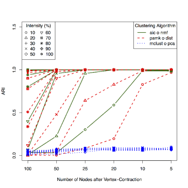
Figure 1: Comparison of three approaches through ARI for the model selection performance. In all cases, our procedure either outperforms or nearly on par with the two baseline algorithms.

4.1.3 Comparison to a non-parametric two-sample test procedure for random graphs

In this section, we consider a sequence of undirected loop-less (unweighted) random graphs $G_{1},\ldots,G_{T}$ such that $\mathbf{E}[G_{t}]$ is an element of a set of $K^{*}$ distinct $n\times n$ matrices whose entries are probabilities. Then, we consider a problem of clustering $T$ graphs into finite number of groups from the data $G_{1},\ldots,G_{T}$. This is an abstraction of a problem in neuroscience, where each $G_{t}$ can represents a copy of neuron-to-neuron interaction pattern, where each $G_{t}$ portraits a different mode of connectivity between neurons. For instance, in Section 4.2, the modes are the chemical and the electrical pathways.

Since each $G(t)$ is undirected and loop-less, its adjacency matrix can be embedded as a vector $X_{t}$ in an element in $\{0,1\}^{n(n-1)/2}$. For our simulation study, we take $T=6$, and take $P_{1}=P_{2}=P_{3}=Q_{1}$ and $P_{4}=P_{5}=P_{6}=Q_{2}$. Then, each $X_{t}$ takes values in $\{0,1\}^{d}$, where $d={100\choose 2}=4950$ for $n=100$. Hence, each $Q_{t}$ is a vector in $(0,1)^{d}$. For our simulation study, we let $n$ to take values in $\{40,60,80,100,120\}$.

For each $t=1,\ldots,T=6$, the matrix $M_{t}=\mathbf{E}[G_{t}]$ is an $n\times n$ block-patterned symmetric matrix such that each $M_{t,ij}\in(0,1)$ and each $G_{t,ij}$ is a Bernoulli random variable with success probability $M_{t,ij}$. Put differently, we simulate each $G_{t}$ according to a (degenerate) stochastic block model, which generalizes the celebrated Erdos-Reyni random graph. The stochastic block model owes its popularity for being a model useful in practice while still being analytic, and we direct the reader’s attention to [9] and [15] for a more detailed treatment.

For our simulation study with $n=100$, we take

$$M_{1}=\begin{bmatrix}[c|c|c|c]B_{11}&B_{12}&B_{13}&B_{14}\\ \cline{1-4}\cr B_{21}&B_{22}&B_{23}&B_{24}\\ \cline{1-4}\cr B_{31}&B_{32}&B_{33}&B_{34}\\ \cline{1-4}\cr B_{41}&B_{42}&B_{43}&B_{44}\end{bmatrix},$$

where each $B_{uv}$ is a $25\times 25$ matrix such that its entries assume the same value $b_{uv}$. Moreover, we set

$$[b_{uv}]=\begin{bmatrix}0.75&0.25&0.25&0.25\\ 0.25&0.75&0.25&0.25\\ 0.25&0.25&0.75&0.25\\ 0.25&0.25&0.25&0.75\end{bmatrix}.$$

Next, we take

$$M_{2}=\begin{bmatrix}[c|c|c]B_{11}^{\prime}&B_{12}^{\prime}&B_{13}^{\prime}\\ \cline{1-3}\cr B_{21}^{\prime}&B_{22}^{\prime}&B_{23}^{\prime}\\ \cline{1-3}\cr B_{31}^{\prime}&B_{32}^{\prime}&B_{33}^{\prime}\end{bmatrix},$$

where the entries of each block $B_{uv}^{\prime}$ assume the same value $b_{uv}^{\prime}$, $B_{11}^{\prime},B_{13}^{\prime},B_{31}^{\prime}$ are $25\times 25$ matrices, and $B_{12}^{\prime}$ and $(B_{23}^{\prime})^{\top}$ are $25\times 50$ matrices. Moreover, we set

$$[b_{uv}^{\prime}]=\begin{bmatrix}0.6&0.4&0.4\\ 0.4&0.6&0.4\\ 0.4&0.4&0.6\end{bmatrix}.$$

Note that, for $M_{1}$, the set of $100$ vertices is partitioned into $4$ groups, and for $M_{2}$, the set of $100$ vertices is partitioned into $3$ groups, where the first and the last groups are composed of $25$ vertices, and the middle group is composed of $50$ vertices.

The adjusted Rand index is used to compare the clustering result of our approach to the ground truth, i.e., $\widehat{K}$ versus $K^{*}$, and $\widehat{\kappa}$ versus $\kappa^{*}$. For each $n$, $100$ Monte Carlo clustering experiments were performed, yielding $100$ adjusted Rand index values, which were averaged. As the number $n$ of vertices takes values in $\{40,60,80,100,120\}$, the average of the values of adjusted Rand index from $100$ Monte Carlo experiments, took values in $\{0.42,0.6,0.8,0.9,0.92\}$ respectively.

To put the aforementioned numeric result in a context, we compare our approach to a non-parametric two-sample test approach of [16] for comparing graphs. To be self-contained, we briefly outline the steps of the two-sample test approach of [16] for comparing graphs. Specifically, first, using the singular value decomposition of each $G(t)$, $n$ vertices were embedded as $n$ points $(Y_{i}(t))_{i=1}^{n}$ in a Euclidean space with its dimension much less $n$, and then for each pair $(t,s)$ with $1\leq t<s=T=6$, the technique in [16] was used to compute the $p$-value $p(t,s)$ for testing whether or not the (empirical) density for $(Y_{i}(t))_{i=1}^{n}$ and the (empirical) density for $(Y_{i}(s))_{i=1}^{n}$ are identically distributed. Then, define $D$ to be the $6\times 6$ hollow symmetric matrix such that $D_{ts}=p(t,s)$ for $t<s$, and subsequently, a technique akin to the principal component analysis is applied to $D$ and then a $K$-means clustering algorithm is used to cluster six “graphs”. For a more detailed description and analysis of the algorithm, we direct the reader to [16], where the testing procedure is shown to be consistent as $n\rightarrow\infty$. As before, for each $n$, $100$ Monte Carlo clustering experiments were performed, yielding $100$ adjusted Rand index values, which were averaged. As the number $n$ of vertices takes values in $\{40,60,80,100,120\}$, the average of the values of adjusted Rand index from $100$ Monte Carlo experiments, took values in $\{0.18,0.28,0.33,0.38,0.39\}$ respectively.

Table III: Averaged value of ARI from a Monte Carlo experiment comparing two graphs

	40	60	80	100	120
aic o nmf	0.42	0.6	0.8	0.9	0.92
two sample	0.18	0.28	0.33	0.38	0.39

As can be seen in Table III, our approach outperforms the non-parametric two-sample approach for each $n=40,60,80,100,120$. On the other hand, this is, to some extend, understandable because the non-parametric two-sample approach uses embedding, and after embedding the algorithm ignores the information that the $i$th vertex in $G(t)$ is also the $i$th vertex in $G(s)$ for any $t<s$. In other words, an advantage of the non-parametric two-sample algorithm is that it can apply to a problem even when the vertex correspondence between vertices of $G(t)$ and the vertices of $G(s)$ is unknown, but in our present situation, the advantage becomes a disadvantage.

To this end, to make a more fair comparison, we modify our original problem slightly so that given $n$ vertices, we are allowed to assume the knowledge of the vertex correspondence across $T$ graphs only for some vertices. Then, for our approach only, to rectify the issue of unknown correspondence, we apply the technique known as the “seeded” graph matching algorithm of [17] to best extrapolate the unknown correspondence, before applying our approach. Specifically, given the number $n$ of vertices, we step the number $m$ of the known vertices toward $n$ in an increment of $5$.

The result is illustrated in Figure 2, where for compactness, MT abbreviates Multiple hypothesis Testing for the non-parametric two-sample approach, and NL abbreviates Non-zero penalizing weighted Likelihood for our model selection criterion, i.e., (aic o nmf). In summary, for each $n$, when $m$ is small, the non-parametric two-sample test approach outperforms our approach, but when $m$ is moderate or large, our approach outperforms the non-parametric two-sample test approach. The low values of the adjusted Rand index for our approach when $m/n\approx 0$ and for the non-paramaetric two-sample test approach when $m/n\approx 1$ are understandable. We conjecture that the location at which the values of the adjusted Rand index for two approaches cross over is a property of the underlying “seeded graph matching” algorithm of [17], but a deep analysis of this phenomenon is beyond the scope of our present work.

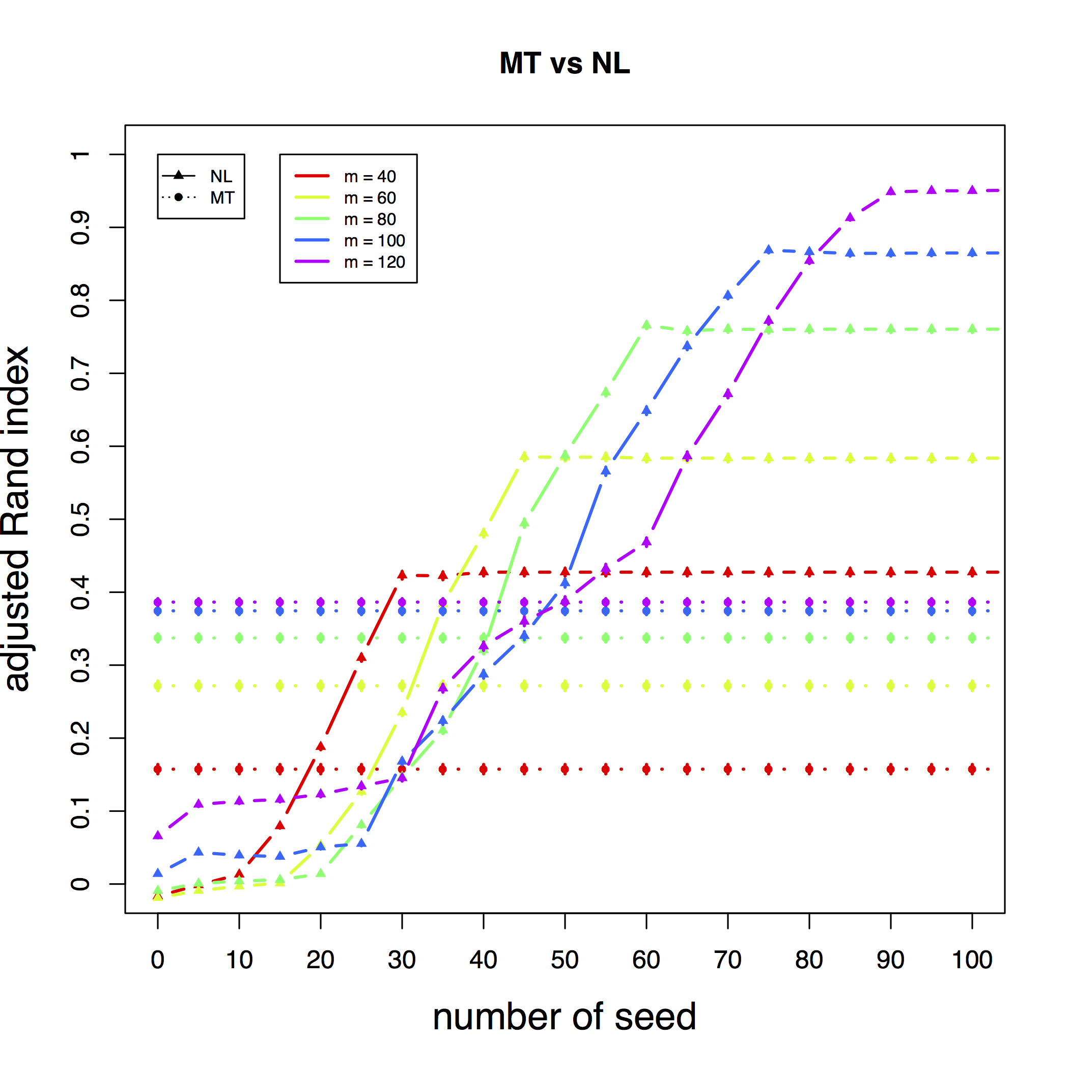
Figure 2: Comparison of two clustering algorithms, specifically, the two-sample test procedure (MT) in [16] and our clustering approach (NL) which is (aic o nmf) When the vertex correspondence is fully known, our approach outperforms, but when no vertex correspondence is known, the non-parametric two sample procedure outperforms. When only fraction of the true correspondence is known, the unknown correspondence is extrapolated from the known correspondence from the connectivity pattern, using the “seeded” graph matching algorithm from [17].

4.2 C. elegan connectomics

In [18], to study the decision-making process of the C. elegan, chemical and electrical neuronal pathways of a C. elegan worm’s $279$ neurons were observed, yielding a pair of graphs on the same (matching) vertex set. First, $279$ neurons are collapsed according to their types, yielding a pair of graphs on $3$ vertices. This yields a $3\times 2$ matrix $X$, where each row corresponds to a pair of vertices (collapsed neurons), and the two columns correspond to two types of pathways. Our clustering approach yields that the value of $\Delta(K)$ for $K=1$ and $K=2$ are $7.79$ and $7.69$, suggesting $\widehat{K}=2$. Next, to allow for a larger dimension while avoiding working with an excessively sparse matrix, vertex contraction is performed so that for each of the first eight groups of thirty neurons, its thirty neurons are aggregated (collapsed) to a single vertex, and then, the remaining thirty-nine vertices are aggregated to a single vertex. These groupings do not signify any special feature. This yields a pair of weighted graphs on $9$ vertices, whence the corresponding matrix $X$ is $36\times 2$ matrix $X$, because $36={9\choose 2}$. Performing our clustering procedure to the matrix yields that the values of $\Delta(K)$ for $K=1$ and $K=2$ are $15.84$ and $15.61$, suggesting that there are two patterns. In words, our approach suggests that the chemical pathways and electric pathways of the C. elegan worm were sufficiently different with respect to their connectivity patterns during the period of observation, corroborating the visual patterns observed in Figure 3.

Figure 3: Connectivity matrices for C. elegan’s chemical and electrical networks between neurons. Visually, while there are similarities between the graphs representing two networks, it can be seen that there are also dissimilarities. Our numerical experiment yields that $\widehat{K}=2$, further corroborating that two networks are sufficiently different.

4.3 Swimmer Dataset

The swimmer data set is a frequently-tested data set for bench-marking NMF algorithms (c.f. [1] and [19]). In our present notation, each column of $220\times 256$ data matrix $X$ is a vectorization of a binary image, and each row corresponds to a particular pixel. Each image is a binary images ($20$-by-$11$ pixels) of a body with four limbs which can be positioned in four different positions. As such, in the language of [19], it can be seen that the matrix $X$ is $16$-separable, or equivalently, the (minimal) inner dimension of $X$ is $16$. However, as it so happens, the rank of $X$ is $13$. In other words, there are $16$ basic patterns/motifs in $X$ that are repeated, and the rank of $X$ being $13$ is a nuisance fact. As displayed in Table IV, the value of $\Delta(K)$ is minimized at $K=16$, matching the inner dimension of $X$.

Table IV: Values of $\Delta(K)$ for estimating the inner dimension for the Swimmer dataset

$K$	$D(\widehat{\mathcal{Q}},\widehat{\kappa})$	penalty	$\Delta(K)$
1	997.87	0.00	997.87
2	986.32	0.02	986.34
3	982.11	0.05	982.16
4	982.94	0.08	983.02
5	982.16	0.10	982.27
6	979.66	0.14	979.80
7	973.32	0.16	973.49
8	967.80	0.20	967.99
9	958.16	0.27	958.42
10	957.31	0.31	957.62
11	957.71	0.31	958.02
12	947.05	0.35	947.40
13	907.26	0.32	907.58
14	889.82	0.51	890.32
15	865.97	0.76	866.73
16	834.69	0.91	835.59
17	834.66	4.07	838.73
18	834.65	13.79	848.44
19	834.65	29.27	863.92
20	834.65	10.61	845.27

5 Discussion

Theorem 1, 2, and Theorem 3 are proven under simplifying assumptions. Specifically, a shortcoming of Theorem 3 is that $\mathbf{E}[X]$ has a finite dimensional block structure, while this can be relaxed to other various settings in which the number of blocks can grow. Next, a shortcoming of Theorem 1 and 2 is that our analysis is done with $Q^{*}$, $Q^{*,m}$ and $Q^{*,s}$ rather than their $\operatorname*{MLqE}$ counter-parts. A remedy for this shortcoming is to use a concentration-inequality type argument to show that their counter-parts are concentrated at $Q^{*}$, $Q^{*,m}$ and $Q^{*,s}$ with high probability, but this is beyond the scope of our current work.

As obvious as the form of the penalty term in (9) may seems in retrospect, i.e., not counting the zero entries as a part of parameters, to our best knowledge, surprisingly, there is no literature that addresses this idea as we did. The idea of not counting the zeros is similar to McNemar’s test in the way it is discussed in [20, pg 77], although the similarity is only in sprit. On the other hand, as done in [21], often clustering of multinomial observations is studied in a Bayesian manner, where the prior distribution on a probability vector is specified by a non-degenerate Dirichlet distribution. For such situations, as discussed, our criterion with $(s,\gamma)=(1,1)$ reduces to the conventional AIC.

Beyond data of biological nature akin to our numerical section, our work in this paper can also be considered for various types of data with noise or without noise, which can be expected to be decomposed as a product of two non-negative matrices. For example, a collection of images of single color channel, a collection of documents with various topics and a collection of sensors interaction records are few such examples. A further investigation into how far our approach can be taken to determine the non-negative factorization’s inner dimension, is of interest beyond this work.

Appendix A Proof of Theorem 1

Proof.

First, by way of a Taylor expansion of the $\log$ function, we note

$$\quad\mathbf{E}[\varphi(\widehat{P})]$$ (16)

$$=\varphi(P^{*})-\mathbf{E}[\sum_{i,t}\frac{1}{\overline{n}_{\kappa^{*}(t)}^{2}}P^{*}_{i,t}\bm{1}\{P^{*}_{i,t}>0\}\frac{1}{P^{*}_{i,t}}(\widehat{P}_{i,t}-P^{*}_{i,t})]$$ (17)

$$-\mathbf{E}[\sum_{i,t}\frac{1}{\overline{n}_{\kappa^{*}(t)}^{2}}P^{*}_{i,t}\bm{1}\{P^{*}_{i,t}>0\}\frac{-1}{2(P^{*}_{i,t})^{2}}(\widehat{P}_{i,t}-P^{*}_{i,t})^{2}]$$ (18)

$$-\mathbf{E}[\sum_{i,t}\frac{1}{\overline{n}_{\kappa^{*}(t)}^{2}}R(\widehat{P}_{i,t},P^{*}_{i,t})],$$ (19)

where $R$ denotes the high order remainder term.

Since $\widehat{P}$ is an unbiased estimator of $P^{*}$, we see that the second term on the right in (17) vanishes to zero. For the term in (18), we note that since each $X_{i,t}$ is a binomial random variable for $N_{t}$ trials with its success probability $P^{*}_{i,t}$, we see that

$$\quad-\sum_{i,t}\frac{1}{\overline{n}_{\kappa^{*}(t)}^{2}}\bm{1}\{P^{*}_{i,t}>0\}\frac{-1}{2P^{*}_{i,t}}\mathbf{E}[(\widehat{P}_{i,t}-P^{*}_{i,t})^{2}]$$ (20)

$$=\sum_{i,t}\frac{1}{\overline{n}_{\kappa^{*}(t)}^{2}}\bm{1}\{P^{*}_{i,t}>0\}\frac{1}{2P^{*}_{i,t}}\frac{1}{N_{t}}P^{*}_{i,t}(1-P^{*}_{i,t})$$ (21)

$$=\sum_{i,t}\frac{1}{\overline{n}_{\kappa^{*}(t)}^{2}}\bm{1}\{P^{*}_{i,t}>0\}\frac{1}{2N_{t}}(1-P^{*}_{i,t})$$ (22)

$$=\sum_{t=1}^{T}\frac{1}{\overline{n}_{\kappa^{*}(t)}^{2}}\frac{1}{2N_{t}}\left(\sum_{i}\bm{1}\{P^{*}_{i,t}>0\}\right)$$ (23)

$$\qquad\qquad-\sum_{t=1}^{T}\frac{1}{\overline{n}_{\kappa^{*}(t)}^{2}}\frac{1}{2N_{t}}\left(\sum_{i}\bm{1}\{P^{*}_{i,t}>0\}P^{*}_{i,t}\right)$$ (24)

$$=\sum_{t=1}^{T}\frac{1}{\overline{n}_{\kappa^{*}(t)}^{2}}\frac{\overline{Z}_{\kappa^{*}(t)}}{2N_{t}}-\sum_{t=1}^{T}\frac{1}{\overline{n}_{\kappa^{*}(t)}^{2}}\frac{1}{2N_{t}},$$ (25)

where the last equality is due to the fact that each column of $P^{*}$ sums to one. Hence, in summary, we see that

$$\lim_{\ell\rightarrow\infty}\ell(\mathbf{E}[\varphi(\widehat{P})]-\varphi(P^{*}))=\lim_{\ell\rightarrow\infty}\ell\sum_{t=1}^{T}\frac{\overline{Z}_{\kappa^{*}(t)}-1}{2N_{t}{\overline{n}_{\kappa^{*}(t)}^{2}}}.$$ (26)

Letting $t_{k}$ be any fixed $t\in k(\kappa^{*})$, since $\lim_{\ell\rightarrow\infty}N_{t_{k}}/\ell=\overline{\lambda}_{k}$ by assumption,

$$\lim_{\ell\rightarrow\infty}\ell\sum_{t=1}^{T}\frac{\overline{Z}_{\kappa^{*}(t)}-1}{N_{t}\overline{n}_{\kappa^{*}(t)}^{2}} =\lim_{\ell\rightarrow\infty}\ell\sum_{k=1}^{K^{*}}\overline{n}_{k}\frac{\overline{Z}_{k}-1}{N_{t_{k}}\overline{n}_{k}^{2}}$$ (27)

$$=\sum_{k=1}^{K^{*}}\frac{\overline{Z}_{k}-1}{\overline{n}_{k}\lim_{\ell\rightarrow\infty}N_{t_{k}}/\ell}$$ (28)

$$=\sum_{k=1}^{K^{*}}\frac{\overline{Z}_{k}-1}{\overline{\lambda}_{k}\overline{n}_{k}}.$$ (29)

We next consider $\mathbf{E}[\sum_{i,t}R(\widehat{P}_{i,t},P^{*}_{i,t})]$. Note that

$$\quad R(\widehat{P}_{i,t},P_{i,t}^{*})$$ (30)

$$=\sum_{k=3}^{\infty}\frac{1}{k}\frac{(-1)^{k+1}}{(P^{*}_{i,t})^{k}}|\widehat{P}_{i,t}-P^{*}_{i,t}|^{k}$$ (31)

$$=\frac{-1}{(P^{*}_{i,t})^{3}}(\widehat{P}_{i,t}-P^{*}_{i,t})^{3}\sum_{k=0}^{\infty}\frac{(-1)^{k+1}}{(P^{*}_{i,t})^{k}}\frac{(\widehat{P}_{i,t}-P^{*}_{i,t})^{k}}{k+3}.$$ (32)

Hence,

$$\ell|R(\widehat{P}_{i,t},P_{i,t}^{*})|$$ (33)

$$\leq\frac{\ell}{(P^{*}_{i,t})^{3}}|\widehat{P}_{i,t}-P^{*}_{i,t}|^{3}\sum_{k=0}^{\infty}\frac{1}{(P^{*}_{i,t})^{k}}\frac{|\widehat{P}_{i,t}-P^{*}_{i,t}|^{k}}{k}.$$ (34)

Since $\widehat{P}_{i,t}\rightarrow P^{*}_{i,t}$ almost surely, it can be shown that there exists a constant $c>0$ such that for each sufficiently small $\varepsilon>0$, for sufficiently large $\ell$, with $1-\varepsilon$ probability,

$$\sum_{k=0}^{\infty}\frac{1}{(P^{*}_{i,t})^{k}}\frac{|\widehat{P}_{i,t}-P^{*}_{i,t}|^{k}}{k}\leq c.$$

Moreover, using the third moment formula for a binomial random variable explicitly, we have

$$\qquad\lim_{\ell\rightarrow\infty}\ell\mathbf{E}[|\widehat{P}_{i,t}-P^{*}_{i,t}|^{3}\left|\bm{N}\right.]$$ (35)

$$\leq\lim_{\ell\rightarrow\infty}\ell\frac{1}{N_{t}^{3}}N_{t}P^{*}_{i,t}(1-P^{*}_{i,t})(1-2P^{*}_{i,t})$$ (36)

$$\leq\lim_{\ell\rightarrow\infty}\frac{1}{N_{t}/\ell}P^{*}_{i,t}(1-P^{*}_{i,t})\lim_{\ell\rightarrow\infty}\frac{1-2P^{*}_{i,t}}{N_{t}}=0.$$ (37)

In summary, $\lim_{\ell\rightarrow\infty}\ell\mathbf{E}[R(\widehat{P}_{i,t},P_{i,t}^{*})]=0$. Combining with (26) and (29), this completes our proof. ∎

Appendix B Proof of Theorem 2

We first focus on the under-fitted case. That is, consider $\Delta(K^{*})-\Delta(K^{*}-1)$. First, for $(\kappa^{*},Q^{*})\in\Theta(K^{*})$, we have $\log(f(X;\kappa^{*},Q^{*}))=\sum_{t=1}^{T}\log\binom{N_{t}}{X_{t}}+\sum_{k=1}^{K^{*}}\sum_{i=1}^{d}\sum_{\{t:\kappa^{*}(t)=k\}}X_{it}\log Q^{*}_{ik}$, and similarly, but specializing for merging of the $K^{*}-1$ and $K^{*}$ blocks from the true parameter structure, for $(\kappa,Q)\in\Theta_{K^{*}-1}$ with merging of the $(K^{*}-1)$st and $K^{*}$th clusters,

$$\log(f(X;\kappa,Q))$$

$$= \sum_{t=1}^{T}\log\binom{N_{t}}{X_{t}}+\sum_{k=1}^{K^{*}-2}\sum_{i=1}^{d}\sum_{\{t:\kappa(t)=k\}}X_{it}\log Q_{ik}$$

$$+\sum_{i=1}^{d}\sum_{\{t:\kappa(t)=K^{*}-1\}}X_{it}\log Q_{i,K^{*}-1}$$

$$= \sum_{t=1}^{T}\log\binom{N_{t}}{X_{t}}+\sum_{k=1}^{K^{*}-2}\sum_{i=1}^{d}\sum_{\{t:\kappa^{*}(t)=k\}}X_{it}\log Q^{*}_{ik}$$

$$+\sum_{k=K^{*}-1}^{K^{*}}\sum_{i=1}^{d}\sum_{\{t:\kappa^{*}(t)=k\}}X_{it}\log Q_{i,K^{*}-1}.$$

Hence, it follows that

$$\log(f(X;\kappa^{*},Q^{*}))-\log(f(X;\kappa,Q))$$

$$= \sum_{k=K^{*}-1}^{K^{*}}\sum_{i=1}^{d}\sum_{\{t:\kappa^{*}(t)=k\}}X_{it}\log(Q^{*}_{ik}/Q_{i,K^{*}-1}).$$

Then, by taking the expectation with respect to the probability mass function defined by $f(\cdot|\kappa^{*},Q^{*})$, define

$$\delta^{*,m}(T):= \sum_{k=K^{*}-1}^{K^{*}}\sum_{i=1}^{d}\sum_{\{t:\kappa^{*}(t)=k\}}\frac{\mathbf{E}[X_{it}]}{N_{t}}\log(Q^{*}_{ik}/Q_{i,K^{*}-1})$$

$$= \sum_{k=K^{*}-1}^{K^{*}}\left(n_{k}(\kappa^{*})\sum_{i=1}^{d}Q^{*}_{ik}\log(Q^{*}_{ik}/Q_{i,K^{*}-1})\right),$$

where $n_{k}(\kappa^{*})=\sum_{t=1}^{T}\bm{1}\{\kappa^{*}(t)=k\}=\overline{n}_{k}$.

Next, note that

$$\Delta^{*,m}(K^{*}-1)-\Delta^{*}(K^{*})$$

$$= \sum_{k=K^{*}-1}^{K^{*}}\sum_{i=1}^{d}\sum_{\{t:\kappa^{*}(t)=k\}}\frac{X_{it}}{N_{t}}\log(Q^{*}_{ik}/Q_{i,K^{*}-1})$$

$$+\texttt{penalty}^{*,m}(K^{*}-1)-\texttt{penalty}^{*}(K^{*}).$$

Hence, we have

$$\Delta^{*,m}(K^{*}-1)-\Delta^{*}(K^{*})$$

$$= \sum_{k=K^{*}-1}^{K^{*}}\sum_{i=1}^{d}\sum_{\{t:\kappa^{*}(t)=k\}}\frac{X_{it}}{N_{t}}\log(Q^{*}_{ik}/Q_{i,K^{*}-1})-\delta^{*,m}(T)$$

$$+\texttt{penalty}^{*,m}(K^{*}-1)-\texttt{penalty}^{*}(K^{*})+\delta^{*,m}(T)$$

$$= \sum_{k=K^{*}-1}^{K^{*}}\sum_{i=1}^{d}\sum_{\{t:\kappa^{*}(t)=k\}}\left(\frac{X_{it}}{N_{t}}-\mathbf{E}[\frac{X_{it}}{N_{t}}]\right)\log\left(\frac{Q^{*}_{ik}}{Q_{i,K^{*}-1}}\right)$$

$$+\texttt{penalty}^{*,m}(K^{*}-1)-\texttt{penalty}^{*}(K^{*})+\delta^{*,m}(T).$$

Let

$$\zeta^{*,m}\equiv\sum_{k=K^{*}-1}^{K^{*}}\sum_{i=1}^{d}\sum_{\{t:\in k(\kappa^{*})\}}\left(\frac{X_{it}}{N_{t}}-\mathbf{E}[\frac{X_{it}}{N_{t}}]\right)\log\left(\frac{Q^{*}_{ik}}{Q_{i,K^{*}-1}}\right)$$

and note that almost surely, $\lim_{\ell\rightarrow\infty}\zeta=0$. Now, since

$$\lim_{\ell\rightarrow\infty}\mathbf{P}[{\zeta}^{*,m}+(\texttt{penalty}^{*,m}-\texttt{penalty}^{*}+\delta^{*,m})>0]$$

$$= \lim_{\ell\rightarrow\infty}\mathbf{P}[(\Delta^{*,m}-\Delta^{*})>0]$$

$$= \lim_{\ell\rightarrow\infty}\mathbf{P}[\Delta^{*,m}>\Delta^{*}],$$

to show our claim, it is enough to show that for sufficiently large $\ell$,

$$\texttt{penalty}^{*,m}-\texttt{penalty}^{*}+{\delta^{*,m}}>0.$$

In general, for $(s,\gamma)=(1/2,\log(N))$, as $N\rightarrow\infty$,

$$\quad\texttt{penalty}(K;s,\gamma)$$

$$=\log(N)\sum_{k=1}^{K}\frac{\widehat{Z}_{k}^{{(K)}}-1}{\sqrt{\widehat{N}_{k}^{(K)}}}$$

$$=\frac{\log(N)}{\sqrt{N}}\sum_{k=1}^{K}\left(\frac{1}{\sqrt{\widehat{N}_{k}^{(K)}/N}}(\widehat{Z}_{k}^{{(K)}}-1)\right)\rightarrow 0,$$

whence

$$\lim_{N\rightarrow\infty}\left(\texttt{penalty}^{*,m}-\texttt{penalty}^{*}+{\delta^{*,m}}\right)$$

$$= \sum_{k=K^{*}-1}^{K^{*}}\sum_{i=1}^{d}n_{k}(\kappa^{*})Q^{*}_{ik}\log(Q^{*}_{ik}/Q_{i,K^{*}-1}^{*,m})>0,$$

as desired. This completes the under-fitting case.

For the over-fitting case, let

$$\delta^{*,s}:= \sum_{k=K^{*}}^{K^{*}+1}\sum_{i=1}^{d}\sum_{\{t:\kappa^{*}(t)=k\}}\frac{E[X_{it}]}{N_{t}}\log(Q_{i,K^{*}}^{*}/Q_{ik})$$

$$=\sum_{k=K^{*}}^{K^{*}+1}\left(n_{k}(\kappa^{*})\sum_{i=1}^{d}Q^{*}_{iK^{*}}\log(Q_{i,K^{*}}^{*}/Q_{ik})\right),$$

where $n_{k}(\kappa^{*})=\sum_{t=1}^{T}\bm{1}\{\kappa^{*}(t)=k\}=\overline{n}_{k}$, and let

$$\zeta^{*,s}\equiv\sum_{k=K^{*}}^{K^{*}+1}\sum_{i=1}^{d}{\sqrt{N}}\sum_{t\in k(\kappa^{*,s})}\left(\frac{X_{it}}{N_{t}}-\mathbf{E}[\frac{X_{it}}{N_{t}}]\right)\log(\frac{Q^{*}_{i,K^{*}}}{Q_{i,k}^{*,s}}).$$

Since $Q_{i,k}=Q_{i,K^{*}-1}^{*}$ for each $k\geq K^{*}-1$, we have

$$\delta^{*,s}\equiv 0\text{ and }\zeta^{*,s}\equiv 0.$$

Then, we have

$$\lim_{N\rightarrow\infty}\mathbf{P}[\Delta^{*,s}>\Delta^{*}]$$

$$=\lim_{N\rightarrow\infty}\mathbf{P}[\sqrt{N}{\zeta}^{*,s}+\sqrt{N}(\texttt{penalty}^{*,s}-\texttt{penalty}^{*}+\delta^{*,s})>0]$$

$$=\lim_{N\rightarrow\infty}\mathbf{P}[\sqrt{N}(\texttt{penalty}^{*,s}-\texttt{penalty}^{*})>0].$$

Now,

$$\texttt{penalty}^{*,s}-\texttt{penalty}^{*}$$

$$=\log(N)\sum_{k=1}^{K^{*}+1}\frac{\overline{Z}_{k}(Q^{*,s})-1}{\sqrt{N_{k}^{*,s}}}-\log(N)\sum_{k=1}^{K^{*}}\frac{\overline{Z}_{k}(Q^{*})-1}{\sqrt{N_{k}^{*}}}$$

$$\geq\log(N)\frac{\overline{Z}_{K^{*}+1}(Q^{*,s})-1}{\sqrt{N_{K^{*}+1}^{*,s}}}>0,$$

where $\overline{Z}_{k}(Q^{*,s})$ counts the number of non-zero entries of $Q_{k}^{*,s}$, $N_{k}^{*}=(\sum_{t\in k(\kappa^{*})}N_{t})^{1/2}$,

and $N_{k}^{*,s}=(\sum_{t\in k(\kappa^{*,s})}N_{t})^{1/2}$. Hence,

$$\lim_{N\rightarrow\infty}\sqrt{N}(\texttt{penalty}^{*,s}-\texttt{penalty}^{*})$$

$$\geq\lim_{N\rightarrow\infty}\log(N)\frac{\overline{Z}_{K^{*}+1}(Q^{*,s})-1}{\sqrt{N_{K^{*}+1}^{*,s}/N}}$$

$$\geq\lim_{N\rightarrow\infty}\log(N)\frac{\overline{Z}_{K^{*}+1}(Q^{*,s})-1}{\sqrt{\lim_{N\rightarrow\infty}N_{K^{*}+1}^{*,s}/N}}=\infty.$$

Hence, it follows that, as desired,

$$\quad\lim_{\ell\rightarrow\infty}\mathbf{P}[\Delta^{*,s}>\Delta^{*}]$$

$$=\mathbf{P}[\lim_{N\rightarrow\infty}\sqrt{N}(\texttt{penalty}^{*,s}-\texttt{penalty}^{*})>0]=1.$$

This completes our proof.

As a side note, we finish by observing that the last part of our argument can be slightly generalized. Specifically, by the central limit theorem (CLT), as $N\rightarrow\infty$,

$$\sum_{\{t:\kappa(t)=k\}}\frac{(X_{it}/N_{t}-Q^{*}_{ik})}{\sqrt{Q^{*}_{ik}(1-Q^{*}_{ik})/N_{t}}}\implies\mathcal{N}(0,1),$$

where the convergence is in distribution, and similarly, we have as $N\rightarrow\infty$,

$$\sum_{\{t:\kappa(t)=k\}}\sqrt{N_{t}}{(X_{it}/N_{t}-Q^{*}_{ik})}\implies\mathcal{N}(0,Q^{*}_{ik}(1-Q^{*}_{ik})),$$

where $\mathcal{N}(0,Q^{*}_{ik}(1-Q^{*}_{ik}))$ denotes a normal random variable with mean zero and variance $Q^{*}_{ik}(1-Q^{*}_{ik})$. In fact, by the multivariate CLT, we have that as $N\rightarrow\infty$, $\zeta^{*,s}$ converges to a linear combination of normal random variables with mean zero even when $Q_{K^{*}}^{*,s}$ and $Q_{K^{*}}^{*,s}$ may not equal the value of $Q_{K^{*}}^{*}$. This allows one to extend the last part of the over-fitting case. ∎

Appendix C Proof of Theorem 3

We first start with the following lemma.

Lemma 1.

For each $n$, $T$ and $C$,

$$\frac{1}{\sqrt{dT}}\mathbf{E}[\|\widehat{Y}-\mathbf{E}[X]\|_{F}]$$ (38)

$$\leq \ C\sqrt{r}\left(\gamma_{1}\left(\frac{{d}}{T^{3}}\right)^{1/4}+\gamma_{2}\frac{\left(\log(T)\right)^{1/2}}{T}\right)$$ (39)

$$\quad+\sqrt{\frac{1}{dT}\sum_{i,t}\left(\mathbf{E}[(X_{i,t}-C)^{+}]\right)^{2}},$$ (40)

where $\gamma_{1},\gamma_{2},\gamma_{3}$ are (universal) constants that do not depend on $C$, $n$ and $T$ and $(X_{i,t}-C)^{+}=\max\{X_{i,t}-C,0\}$.

Proof.

Let

$$\operatorname*{MSE}(\widehat{Y}):=\frac{1}{dT}\sum_{i,t}(\widehat{Y}_{i,t}-\mathbf{E}[Y_{i,t}])^{2}.$$

By a triangular inequality, we have

$$\frac{1}{\sqrt{dT}}\mathbf{E}[\|\widehat{Y}-\mathbf{E}[X]\|_{F}]$$

$$\leq \frac{1}{\sqrt{dT}}\mathbf{E}[\|\widehat{Y}-\mathbf{E}[Y]\|_{F}]+\frac{1}{\sqrt{dT}}\|\mathbf{E}[Y]-\mathbf{E}[X]\|_{F}$$

$$\leq \sqrt{\operatorname*{MSE}(\widehat{Y})}+\sqrt{\frac{1}{dT}\|\mathbf{E}[Y]-\mathbf{E}[X]\|_{F}^{2}}$$

$$\leq \sqrt{C^{2}\left(\frac{1}{C^{2}}\operatorname*{MSE}(\widehat{Y})\right)}+\sqrt{\frac{1}{dT}\|\mathbf{E}[Y]-\mathbf{E}[X]\|_{F}^{2}}.$$

Now, by [3, Theorem 1.1 & 1.3], for some fixed (universal) constant $\gamma_{1},\gamma_{2}$ (in particular, not depending on $C$, $n$ and $T$), we have

$$\frac{1}{C^{2}}\operatorname*{MSE}(\widehat{Y}) \leq\gamma_{1}\sqrt{r}\left(\frac{{d}}{T^{3}}\right)^{1/4}$$ (41)

$$\qquad+\gamma_{2}\frac{\sqrt{r}}{d^{1/2}T^{1/2}}\left(\frac{d\log(T)}{T}\right)^{1/2}.$$ (42)

On the other hand,

$$\|\mathbf{E}[X-Y]\|_{F}^{2} =\sum_{i,t}\left(\mathbf{E}[X_{i,t}-Y_{i,t};X_{i,t}>C]\right)^{2}$$

$$=\sum_{i,t}\left(\mathbf{E}[(X_{i,t}-C)^{+}]\right)^{2},$$

where in the second equality, we have used the fact that on the event $\{X_{ij,t}\leq C\}$, we have $X_{ij,t}=Y_{ij,t}$ for all $ij$ and $t$. Our claim follows from this. ∎

Proof of Theorem 3.

By assumption, we have

$$0=\lim_{d\wedge T\rightarrow\infty}C_{d,T}\left(\gamma_{1}\left(\frac{{d}}{T^{3}}\right)^{1/4}+\gamma_{2}\frac{\left(\log(T)\right)^{1/2}}{T}\right).$$

Next, to complete our proof, it is enough to show that $\lim_{d\wedge T\rightarrow\infty}e(d,T)=0$, where

$$e(d,T):=\sqrt{\frac{1}{dT}\sum_{i,t}\left(\mathbf{E}[(X_{i,t}-C_{d,T})^{+}]\right)^{2}}.$$

Note that for sufficiently large values of $d\wedge T$, $C_{d,T}\geq(\mathbf{E}[X_{i,t}])$, and we have

$$\qquad\mathbf{E}[(X_{i,t}-C_{d,T})^{+}]$$

$$=\sum_{m=C_{d,T}+1}^{\infty}(m-C_{d,T})\frac{(\mathbf{E}[X_{i,t}])^{m}}{m!}\exp(-(\mathbf{E}[X_{i,t}]))$$

$$=(\mathbf{E}[X_{i,t}])\sum_{m=C_{d,T}+1}^{\infty}\frac{(\mathbf{E}[X_{i,t}])^{m-1}}{(m-1)!}\exp(-(\mathbf{E}[X_{i,t}]))$$

$$\qquad\qquad-C_{d,T}\sum_{m=C_{d,T}+1}^{\infty}\frac{(\mathbf{E}[X_{i,t}])^{m}}{m!}\exp(-(\mathbf{E}[X_{i,t}]))$$

$$\leq C_{d,T}\sum_{m=C_{d,T}}^{\infty}\frac{(\mathbf{E}[X_{i,t}])^{m}}{m!}\exp(-(\mathbf{E}[X_{i,t}]))$$

$$\qquad\qquad-C_{d,T}\sum_{m=C_{d,T}+1}^{\infty}\frac{(\mathbf{E}[X_{i,t}])^{m}}{m!}\exp(-(\mathbf{E}[X_{i,t}]))$$

$$\leq C_{d,T}\frac{(\mathbf{E}[X_{i,t}])^{C_{d,T}}}{C_{d,T}!}\exp(-(\mathbf{E}[X_{i,t}]))$$

$$=(\mathbf{E}[X_{i,t}])\frac{(\mathbf{E}[X_{i,t}])^{C_{d,T}-1}}{(C_{d,T}-1)!}\exp(-(\mathbf{E}[X_{i,t}])).$$

Then,

$$\frac{1}{|\mathcal{B}|}\sum_{i,t}(\mathbf{E}[(X_{i,t}-C_{d,T})^{+}])^{2}$$

$$\leq\frac{1}{|\mathcal{B}|}\sum_{i,t}(\mathbf{E}[X_{i,t}])^{2}\exp(-2(\mathbf{E}[X_{i,t}]))\left(\frac{(\mathbf{E}[X_{i,t}])^{C_{d,T}-1}}{(C_{d,T}-1)!}\right)^{2}$$

$$=\frac{1}{|\mathcal{B}|}\sum_{b=1}^{B}|\mathcal{B}_{b}|\nu_{b}^{2}\exp(-2\nu_{b})\left(\frac{\nu_{b}^{C_{d,T}-1}}{(C_{d,T}-1)!}\right)^{2}$$

$$=\sum_{b=1}^{B}\frac{|\mathcal{B}_{b}|}{|\mathcal{B}|}\nu_{b}^{2}\exp(-2\nu_{b})\left(\frac{\nu_{b}^{C_{d,T}-1}}{(C_{d,T}-1)!}\right)^{2}.$$

Then, $\lim_{d\wedge T\rightarrow\infty}e(n,T)=0$ since

$$0\leq\limsup_{d\wedge T\rightarrow\infty}\frac{1}{|\mathcal{B}|}\sum_{i,t}(\mathbf{E}[(X_{i,t}-C_{d,T})^{+}])^{2}$$

$$=\sum_{b=1}^{B}p_{b}\limsup_{d\wedge T\rightarrow\infty}\left(\nu_{b}^{2}\exp(-2\nu_{b})\left(\frac{\nu_{b}^{C_{d,T}-1}}{(C_{d,T}-1)!}\right)^{2}\right)=0.$$

∎

Appendix D Derivation of an objective function for computing $\operatorname*{MLqE}$ via a Markov chain Monte Carlo method

Fix $q<1$ and $\kappa:\{1,\ldots,T\}\rightarrow\{1,\ldots,K\}$. We let $\mathcal{Q}$ to be the free variables. Now, given $X_{1},X_{2},\ldots,X_{T}$, we let

$$L(\kappa,\mathcal{Q}) =\frac{1}{1-q}\sum_{t=1}^{T}\sum_{i=1}^{d}X_{i}(t)Q_{i,\kappa(t)}^{1-q},$$

$$=\frac{1}{1-q}\sum_{k=1}^{K}\sum_{i=1}^{d}\left(\sum_{\{t:\kappa(t)=k\}}X_{i}(t)\right)Q_{i,k}^{1-q},$$

where for each $k=1,\ldots,K$, $\sum_{i=1}^{d}Q_{i,k}=1$. Then, formulating the problem using the first order KKT condition reduces the problem of maximizing $L(\kappa,\mathcal{Q})$ with respect to $\mathcal{Q}$ to maximizing

$$\frac{1}{1-q}\sum_{k=1}^{K}\sum_{i=1}^{d}M_{i,k}Q_{i,k}^{1-q}+\sum_{k=1}^{K}\mu_{k}\left(1-\sum_{i=1}^{d}Q_{i,k}\right),$$

where $\mu_{1},\ldots,\mu_{K}$ denote the Lagrange multipliers and we write $M_{i,k}=\left(\sum_{\{t:\kappa(t)=k\}}X_{i}(t)\right)$.

Specifically, taking a derivative with respect to each $Q_{k,i}$ yields the condition that for each $k,i$,

$$0=M_{i,k}Q_{i,k}^{-q}+\mu_{k}(-1),$$

whence we have $\mu_{k}^{1/q}Q_{i,k}=M_{i,k}^{1/q}$, $\mu_{k}^{1/q}=\sum_{i=1}^{d}M_{i,k}^{1/q}$ and from this observation, we set

$$\widehat{Q}_{i,k}:=\frac{M_{i,k}^{1/q}}{\sum_{i=1}^{d}M_{i,k}^{1/q}}.$$

Now, let

$$L^{*}(\kappa;q)=\sum_{k=1}^{K}\sum_{i=1}^{d}M_{i,k}\left(\frac{M_{i,k}^{1/q}}{\sum_{j=1}^{d}M_{k,j}^{1/q}}\right)^{1-q},$$ (43)

where the dependence of $M_{i,k}$ on $\kappa$ is implicitly stated. Also, performing a similar sequence of computations, for $q=1$, i.e., for the maximum likelihood estimator, we have

$$L^{*}(\kappa;q)=\sum_{k=1}^{K}\sum_{i=1}^{d}M_{i,k}\log\left(\frac{M_{i,k}}{\sum_{j=1}^{d}M_{k,j}}\right).$$ (44)

Then, taking $\kappa$ as a free variable, the values of $L^{*}(\kappa;q)$ can be explored over all $\kappa\in\{1,\ldots,K\}^{T}$ using any Markov chain Monte Carlo method, for example, by a Gibbs sampling approach. We leave to the reader the remaining details for a Gibbs sampling procedure in which at each step, a single coordinate of $\kappa$ can be changed.

Appendix E Connection to the conventional AIC and BIC

In this section, we show that the form of the penalty term in (9) reduces to the conventional AIC and BIC criteria under some simplifying conditions.

Specifically, we assume in this section that $N_{0}=N_{1}=N_{2}=\cdots=N_{T}>0$ and for each $K$, that $\widehat{Q}_{ik}^{(K)}>0$ for all $i=1,\ldots,d$ and $k=1,\ldots,K$.

First, to see a connection to the conventional AIC criterion in (7), we note that

$$N_{0}\Delta(K)$$

$$=-\sum_{t=1}^{T}\sum_{i=1}^{d}X_{it}\log(\widehat{Q}_{i\widehat{\kappa}(t)}^{(K)})+N_{0}\texttt{penalty}(K;1,1),$$

where

$$N_{0}\texttt{penalty}(K;1,1)=\sum_{k=1}^{K}\left(\widehat{Z}_{k}^{(K)}-1\right)=dK-K.$$

Hence, for some constant $C$ that depends on only the value of $X$,

$$N_{0}\Delta(K)=C-\log(f_{X}(X|\widehat{\theta}(K)))+\texttt{penalty}_{\operatorname*{AIC}}(K),$$

which differs from the one in (7) by the additive constant $C$.

Next, to see a connection to the conventional BIC criterion in (8), we note that when $\gamma=\log(N)/\sqrt{N_{0}}$ and $s=1/2$,

$$N_{0}\Delta(K)=-\log(f_{X}(X|\widehat{\theta}(K)))+N_{0}\texttt{penalty}(K;\gamma,1/2).$$

Then, we have

$$N_{0}\texttt{penalty}(K;\gamma,1/2)=\log(N)(dK-K).$$

Hence,

$$N_{0}\Delta(K)=C-\log(f_{X}(X|\widehat{\theta}(K)))+\texttt{penalty}_{\operatorname*{BIC}}(K),$$

which differs from the one in (8) by the additive constant $C$.

Acknowledgment

This work is partially supported by Johns Hopkins University Armstrong Institute for Patient Safety and Quality and the XDATA program of the Defense Advanced Research Projects Agency (DARPA) administered through Air Force Research Laboratory contract FA8750-12-2-0303. We thank Youngser Park for his assistance in performing numerical experiments. We thank the anonymous referees for their valuable comments.

References

• [1] D. Donoho and V. Stodden, “When does non-negative matrix factorization give a correct decomposition into parts?” in Advances in Neural Information Processing Systems 16.   MIT Press, 2004, pp. 1141–1148.
• [2] D. Ferrari and Y. Yang, “Maximum Lq-likelihood estimation,” Ann. Statist., vol. 38, no. 2, pp. 753–783, 04 2010. [Online]. Available: http://dx.doi.org/10.1214/09-AOS687
• [3] R. H. Keshavan, A. Montanari, and S. Oh, “Matrix completion from noisy entries,” The Journal of Machine Learning Research, vol. 99, pp. 2057–2078, 2010.
• [4] S. Chatterjee, “Matrix estimation by universal singular value thresholding,” arXiv preprint arXiv:1212.1247, 2013. [Online]. Available: http://arxiv.org/abs/1212.1247
• [5] H. Kim and H. Park, “Nonnegative matrix factorization based on alternating nonnegativity constrained least squares and active set method,” SIAM Journal on Matrix Analysis and Applications, vol. 30, no. 2, pp. 713–730, 2008.
• [6] M. W. Berry, M. Browne, A. N. Langville, V. P. Pauca, and R. J. Plemmons, “Algorithms and applications for approximate nonnegative matrix factorization,” Computational statistics & data analysis, vol. 52, no. 1, pp. 155–173, 2007.
• [7] J.-P. Brunet, P. Tamayo, T. R. Golub, and J. P. Mesirov, “Metagenes and molecular pattern discovery using matrix factorization,” Proceedings of the National Academy of Sciences, vol. 101, no. 12, pp. 4164–4169, 2004. [Online]. Available: http://www.pnas.org/content/101/12/4164.abstract
• [8] H. Linhart and W. Zucchini, Model selection, ser. Wiley series in probability and mathematical statistics: Applied probability and statistics.   Wiley, 1986.
• [9] Y. Wang and P. J. Bickel, “Likelihood-based model selection for stochastic block models,” arXiv preprint arXiv:1502.02069, 2015.
• [10] R. O. Duda and P. E. Hart, Pattern Classification and Scene Analysis.   John Willey & Sons, 1973.
• [11] P. J. Rousseeuw, “Silhouettes: a graphical aid to the interpretation and validation of cluster analysis,” Journal of computational and applied mathematics, vol. 20, pp. 53–65, 1987.
• [12] M. Zhu and A. Ghodshi, “Automatic dimensionality selection from the scree plot via the use of profile likelihood,” Computational Statistics & Data Analysis, vol. 51, pp. 918–930, 2006.
• [13] C. Fraley and A. E. Raftery, “Model-based clustering, discriminant analysis and density estimation,” Journal of the American Statistical Association, vol. 97, pp. 611–631, 2002.
• [14] W. Rand, “Objective criteria for the evaluation of clustering methods,” Journal of the American Statistical Association, 1971.
• [15] D. M. Pavlovic, P. E. Vértes, E. T. Bullmore, W. R. Schafer, and T. E. Nichols, “Stochastic blockmodeling of the modules and core of the Caenorhabditis elegans connectome,” PloS one, vol. 9, no. 7, p. e97584, 2014.
• [16] M. Tang, A. Athreya, D. L. Sussman, V. Lyzinski, and C. E. Priebe, “A nonparametric two-sample hypothesis testing problem for random dot product graphs,” arXiv preprint arXiv:1409.2344, 2014.
• [17] V. Lyzinski, D. L. Sussman, D. E. Fishkind, H. Pao, J. T. Vogelstein, and C. E. Priebe, “Seeded graph matching for large stochastic block model graphs,” Parallel Computing, 2015.
• [18] T. A. Jarrell, Y. Wang, A. E. Bloniarz, C. A. Brittin, M. Xu, J. N. Thomson, D. G. Albertson, D. H. Hall, and S. W. Emmons, “The connectome of a decision-making neural network,” Science, vol. 337, no. 6093, pp. 437–444, 2012.
• [19] N. Gillis and R. Luce, “Robust near-separable nonnegative matrix factorization using linear optimization,” Journal of Machine Learning Research, pp. 1249–1280, 2014.
• [20] B. D. Ripley, Pattern recognition and neural networks.   Cambridge university press, 1996.
• [21] N. Bouguila, “Clustering of count data using generalized Dirichlet multinomial distributions,” Knowledge and Data Engineering, IEEE Transactions on, vol. 20, no. 4, pp. 462–474, 2008.