Nonparametric Inference For Density Modes
Christopher R. Genovese, Marco Perone-Pacifico,
Isabella Verdinelli and Larry Wasserman
Carnegie Mellon University and University of Rome

December 29, 2013

We derive nonparametric confidence intervals for the eigenvalues of the Hessian at modes of a density estimate. This provides information about the strength and shape of modes and can also be used as a significance test. We use a data-splitting approach in which potential modes are identified using the first half of the data and inference is done with the second half of the data. To get valid confidence sets for the eigenvalues, we use a bootstrap based on an elementary-symmetric-polynomial (ESP) transformation. This leads to valid bootstrap confidence sets regardless of any multiplicities in the eigenvalues. We also suggest a new method for bandwidth selection, namely, choosing the bandwidth to maximize the number of significant modes. We show by example that this method works well. Even when the true distribution is singular, and hence does not have a density, (in which case cross validation chooses a zero bandwidth), our method chooses a reasonable bandwidth.

Key words: bootstrap, density estimation, modes, persistence.

1 Introduction

Figure 1 shows a one-dimensional density estimate with two modes. The leftmost mode is likely to correspond to a real mode in the true density. But the second smaller mode on the right may be due to random fluctuation. How can we tell a real mode from random fluctuation? In this paper, we provide a simple hypothesis test to answer this question that is easy to implement, even in multivariate problems. The basic idea is this: a confidence interval for the second derivative of the density will be strictly negative for the left mode but is likely to cross 0 for the right mode.

Let $Z_{1},\ldots,Z_{n}\in\mathbb{R}^{d}$ be a sample from a distribution $P$ with density $p$. We assume that the gradient $g$ and Hessian ${\cal H}$ of $p$ are bounded continuous functions. Furthermore, we assume that $p$ has finitely many, well-separated modes $m_{1},\ldots,m_{k_{0}}$. We do not assume that $k_{0}$ is known. Our goal is to estimate the modes and to give confidence sets that provide shape information about the estimated modes.

There are many reasons for mode hunting and many methods to find modes; see, for example, Klemelä (2009); Li et al. (2007); Dümbgen and Walther (2008). In particular, modes can be used as the basis of nonparametric clustering (Chacón, 2012; Chazal et al., 2011; Comaniciu and Meer, 2002; Fukunaga and Hostetler, 1975; Li et al., 2007).

There are several difficulties in defining tests for modes. Consider a point $x\in\mathbb{R}^{d}$ and suppose we want to test

$$H_{0}:\ x\ \mbox{is not a mode\ of }p\ \ \ \ \ \ \ \ \mbox{versus}\ \ \ \ \ \ \ \ H_{1}:\ x\ \mbox{is a mode\ of }p.$$

First, testing the null hypothesis of “no mode” raises problems, analogous to testing the null that a mean is not zero, because the alternative forms a measure zero set. More precisely, if $\nabla p(x)\equiv g(x)=(g_{1}(x),\ldots,g_{d}(x))^{T}$ is the gradient of $p$ at $x$, $\lambda_{1}(x)\geq\cdots\geq\lambda_{d}(x)$ are the eigenvalues of the Hessian ${\cal H}(x)$, and $\Omega=\mathbb{R}\times\mathbb{R}^{d}$, then $H_{0}=\Omega-H_{1}$ and

$$H_{1}=\Bigl{\{}(\lambda_{1},g)\in\Omega:\ \lambda_{1}<0,\ g=(0,\ldots,0)^{T}\Bigr{\}}.$$

is a measure zero subset of $\Omega$. No meaningful test can be constructed of such a “reverse null hypothesis.” The second problem is that there are uncountably many possible locations at which a mode can occur, leading potentially to a difficult multiple testing problem. Finally, verifying that a mode exists requires making inference about eigenvalues of the Hessian. But the eigenvalues are not continuously differentiable functions of the Hessian which makes methods like the bootstrap and the delta method invalid.

Figure 1: The mode on the left appears to be real. The mode on the right might be due to random fluctuation.

We overcome these problems by combining several ideas:

1. We use data splitting to separate the process of finding candidate modes from the process of hypothesis testing. This ameliorates the multiplicity problem and simplifies the hypothesis test as well. Specifically, assume that the sample size is $2n$ and randomly split the data into two halves $X=(X_{1},\ldots,X_{n})$ and $Y=(Y_{1},\ldots,Y_{n})$.

2. In stage one, we use $X$ to find a finite set of candidate modes $\widehat{\cal M}$.

3. In stage two, we use the second half of the data $Y$ to estimate the Hessian of the density at the candidate modes $\widehat{\cal M}$. We transform the eigenvalues of the Hessian using elementary symmetric polynomials (ESP). As noted in Beran and Srivastava (1985), the bootstrap leads to asymptotically valid confidence sets for the transformed eigenvalues. We then invert the mapping to get a valid confidence set for the eigenvalues. This provides useful shape information about the modes, which we call an eigenportrait.

4. The eigenportrait can be used to formulate a test for the importance of the mode. As a surrogate for testing whether a candidate mode is not really a mode, we instead test if $x$ is an “approximate mode”. This requires reformulating $H_{1}$ to capture the idea of an approximate mode. There is no unique way to do this. One possibility is to take $H_{0}=\Omega-H_{1}$ where

   $$H_{1}=\Bigl{\{}(\lambda_{1},g)\in\Omega:\ \lambda_{1}<0,\ ||g||<\delta\Bigr{\}}$$

   where $\delta>0$ is a small positive constant. In practice, the constraint $||g||<\delta$ has no effect on the test since the estimated gradient is 0 at the modes in stage one and hence is likely to be close to 0 in stage two. In practice, therefore, we simplify matters by just testing

   $$H_{0}:\lambda_{1}\geq 0\ \ \ {\rm versus}\ \ \ H_{1}:\lambda_{1}<0.$$

Bias. We will use a kernel density estimator $\widehat{p}_{h}$ depending on a bandwidth $h>0$. In this paper we view $\widehat{p}_{h}$ as an estimator of its mean $p_{h}$. In particular, we view the modes of $\widehat{p}_{h}$ as estimates of the modes of $p_{h}$. Of course, there is a bias (typically of order $O(h^{2})$) that separates $p_{h}$ from $p$. This bias is not of critical importance when studying modes. Instead, our primary concern is the variability of $\widehat{p}_{h}$ as an estimator of $p_{h}$. Including the bias in any inferential procedures for density estimators raises well known complications since the bias is harder to estimate than the density. One can use various devices such as undersmoothing to deal with the bias. These difficulties are a distraction from our main thrust and so we focus on inference for $p_{h}$.

Related Work. There is a large literature on mode finding. Many methods are based on the mean-shift algorithm for finding modes of kernel estimators; see Comaniciu and Meer (2002); Fukunaga and Hostetler (1975). An early paper in the statistics literature on using kernel density estimators for mode hunting is Silverman (1981). He used the observed bandwidth at which a new mode appears as a test for multimodality. The properties of this test are rather complicated, even in one-dimension: see Mammen et al. (1992).

Significance testing for modes of kernel estimators was considered in Godtliebsen et al. (2002) and Duong et al. (2008). The latter reference is very related to this paper. We discuss the differences in our approaches in Section 3. Asymptotic theory and bandwidth selection for mode hunting and derivative estimation is discussed in Chacon and Duong (2013); Chacón and Duong (2010); Chacón et al. (2011). Donoho and Liu (1991) showed that the minimax rate for estimating a mode in one dimension, assuming the density is locally quadratic around the mode, is $O(n^{-1/5})$. Although not stated explicitly in that paper, it is clear that the rate for $d$-dimensional densities is $O(n^{-1/(4+d)})$. Konakov (1974) studied the asymptotics of the mode estimator in the multivariate case. Klemelä (2005) considered adaptive estimation that takes into account the regularity in a neighborhood of a mode. Dümbgen and Walther (2008) presented a method for constructing multiscale confidence intervals for modes but the method is only applicable to one-dimensional densities.

Clustering, based on modes, was used in Chacón (2012) and Li et al. (2007). Chazal et al. (2011) considered a completely different approach to mode-based clustering on persistent homology; we compare this to the current approach in Section 5. Finally, we mention that there is a large literature on the related problem of estimating level sets of density; for example, see Polonik (1995); Cadre (2006); Walther (1997). The concept of excess mass Müller and Sawitzki (1991) provides a link between level sets and modes.

Outline. In Section 2, we discuss mode hunting and mode clustering. We present our hypothesis test in Section 3. A crucial part of the test is a non-standard bootstrap procedure described in Section 4. We compare our approach to persistent homology in Section 5. Section 6 presents some examples. In Section 7, we use our procedure as part of a new method for bandwidth selection for mode hunting. Section 8 presents some theoretical properties of the method. Concluding remarks are in Section 9.

Notation. Given a density function $p$, we use $g(x)$ to denote the gradient of $p$ at $x$ and we use ${\cal H}(x)$ to denote the Hessian of $p$ at $x$. The eigenvalues of ${\cal H}(x)$ are denoted by $\lambda(x)=(\lambda_{1}(x),\ldots,\lambda_{d}(x))$ where $\lambda_{1}(x)\geq\cdots\geq\lambda_{d}(x)$. Since the eigenvalues at a mode are negative, it is convenient to define $\gamma(x)=(\gamma_{1}(x),\ldots,\gamma_{d}(x))$ where $\gamma_{j}(x)=-\lambda_{j}(x)$. For an $n\times r$ matrix $A$, define ${\rm vec}(A)$ to be the $nr\times 1$ column vector obtained by stacking the columns of $A$, that is, ${\rm vec}A=(A_{11},A_{21},\ldots,A_{n1},A_{12},\ldots,A_{nn})^{T}$. Also, for symmetric matrices, ${\rm vech}$ is the vec operator applied only to the upper triangular part of the matrix. For a vector-valued function $f=(f_{1},\ldots,f_{d})$ we follow Chacón et al. (2011), by defining $D^{\otimes r}f$ as

$$D^{\otimes r}f(x)=\left(\begin{array}[]{c}D^{\otimes r}f_{1}(x)\\ \vdots\\ D^{\otimes r}f_{d}(x)\end{array}\right).$$

Here, $D^{\otimes r}$ denotes the $r^{\rm th}$ derivative. Then, for the Hessian ${\cal H}f=\partial^{2}f/(\partial x\partial x^{T})$ we have ${\rm vec}\,{\cal H}f=D^{\otimes 2}f$. In the special case $r=1$ we usually just write $\nabla f$ for the gradient. Also, we sometimes use $\nabla^{(2)}$ for the second derivative. The largest eigenvalue of a matrix $A$ is denoted by $\lambda_{1}(A)$. We use $C$ to denote a generic positive constant.

Assumptions. Throughout the paper we make the following assumptions.

(A1) The density $p$ is a bounded, continuous density supported on a compact set ${\cal X}\subset\mathbb{R}^{d}$.

(A2) The gradient $g$ and Hessian ${\cal H}$ of $p$ are bounded and continuous. The Hessian is non-degenerate at all stationary points.

(A3) $p$ has finitely many modes $m_{1},\ldots,m_{k_{0}}$ in the interior of ${\cal X}$.

(A4) Let

$$\Delta=\min_{s\neq t}||m_{s}-m_{t}||\ \ \ \ \ \mbox{and}\ \ \ \ \ L=\max_{1\leq j\leq k_{0}}\lambda_{1}({\cal H}(m_{j})).$$ (1)

We assume that $\Delta>0$ and $L<0$.

(A5) The kernel $K$ used in the density estimator is a symmetric probability density with bounded and continuous first and second derivatives and bounded second moment.

2 Modes and Clusters

One of our main motivations for finding significant modes is so that they can be used for clustering. Let $m_{1},\ldots,m_{k_{0}}$ be the modes of $p$. Assume that $p$ is a Morse function, which means that the Hessian of $p$ at each stationary point is non-degenerate.

Given any point $x\in\mathbb{R}^{d}$ there is a unique gradient ascent path, or integral curve, passing through $x$ that eventually leads to one of the modes. We define the clusters to be the “basins of attraction” of the modes, the equivalence classes of points whose ascent paths lead to the same mode. Formally, an integral curve through $x$ is a path $\pi_{x}:\mathbb{R}\to\mathbb{R}^{d}$ such that $\pi_{x}(t)=x$ for some $t$ and such that

$$\pi^{\prime}_{x}(t)=\nabla p(\pi_{x}(t)).$$ (2)

Integral curves never intersect (except at stationary points) and they partition the space (Matsumoto (2002)). Equation (2) means that the path $\pi$ follows the direction of steepest ascent of $p$ through $x$. The destination of the integral curve $\pi$ through a (non-mode) point $x$ is defined by

$${\sf dest}(x)=\lim_{t\to\infty}\pi_{x}(t).$$ (3)

(We define ${\sf dest}(m)=m$ for any mode $m$.) It can then be shown that for all $x$, ${\sf dest}(x)=m_{j}$ for some mode $m_{j}$. That is: all integral curves lead to modes. For each mode $m_{j}$, define the sets

$${\cal A}_{j}=\Bigl{\{}x:\ {\sf dest}(x)=m_{j}\Bigr{\}}.$$ (4)

These sets are known as the ascending manifolds, and also known as the cluster associated with $m_{j}$, or the basin of attraction of $m_{j}$. The ${\cal A}_{j}$’s partition the space. See Figure 2.

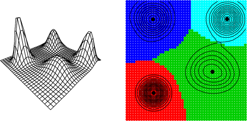
Figure 2: The left plot shows a function with four modes. The right plot shows the ascending manifolds (basins of attraction) corresponding to the four modes.

Given data $X_{1},\ldots,X_{n}$ we construct an estimate $\widehat{p}$ of the density. Let $\widehat{m}_{1},\ldots,\widehat{m}_{k}$ be the estimated modes and let $\widehat{\cal A}_{1},\ldots,\widehat{\cal A}_{k}$ be the corresponding ascending manifolds derived from $\widehat{p}$. The sample clusters $C_{1},\ldots,C_{k}$ are defined to be $C_{j}=\bigl{\{}X_{i}:\ X_{i}\in\widehat{\cal A}_{j}\bigr{\}}$. Before finding clusters, it is important to find out which modes are significant and which are explainable as random fluctuations. This is one of the motivations for the current paper.

We will estimate the density $p$ with the kernel density estimator

$$\widehat{p}(x)\equiv\widehat{p}_{h}(x)=\frac{1}{n}\sum_{i=1}^{n}\frac{1}{h^{d}}\,K\left(\frac{||x-X_{i}||}{h}\right)$$ (5)

where $K$ is a smooth, symmetric kernel and $h>0$ is the bandwidth. The mean of the estimator is

$$p_{h}(x)=\mathbb{E}[\widehat{p}_{h}(x)]=\int K(t)p(x+th)dt.$$ (6)

In general, one can use a bandwidth matrix $H$ in the estimator, with

$$\widehat{p}(x)\equiv\widehat{p}_{H}(x)=\frac{1}{n}\sum_{i=1}^{n}K_{H}(x-X_{i})$$ (7)

where $K_{H}(x)=|H|^{-\frac{1}{2}}K(H^{-\frac{1}{2}}x)$. As discussed in Chacon and Duong (2013) and Chacón et al. (2011), using a non-diagonal matrix can lead to better density estimates than using a diagonal bandwidth matrix. But for simplicity, here we use a single, scalar bandwidth $h$, corresponding to $H=h^{2}I$. As explained in the introduction, in this paper we regard $\widehat{p}_{h}$ as an estimator of $p_{h}$ and we aim to find the modes of $p_{h}$.

To locate the modes of $\widehat{p}_{h}$ we use the mean shift algorithm ((Fukunaga and Hostetler, 1975; Comaniciu and Meer, 2002)), which finds modes by approximating the steepest ascent paths. (Arias-Castro et al. (2013)). The algorithm is given in Figure 3. The result of this process is a set of candidate modes $\widehat{\cal M}=\{\widehat{m}_{1},\ldots,\widehat{m}_{k}\}$. Note that $k$ is random since it is the observed number of modes of the density estimator.

Mean Shift Algorithm
1. Input: $\widehat{p}(x)$ and a mesh of points $A=\{a_{1},\ldots,a_{N}\}$ (often taken to be the data points). 2. For each mesh point $a_{j}$, set $a_{j}^{(0)}=a_{j}$ and iterate the following equation until convergence: $$a_{j}^{(s+1)}\longleftarrow\frac{\sum_{i=1}^{n}X_{i}K\left(\frac{||a_{j}^{(s)}-X_{i}||}{h}\right)}{\sum_{i=1}^{n}K\left(\frac{||a_{j}^{(s)}-X_{i}||}{h}\right)}.$$ 3. Let $\widehat{\cal M}$ be the unique values of the set $\{a_{1}^{(\infty)},\ldots,a_{N}^{(\infty)}\}$. 4. Output: $\widehat{\cal M}$.

Figure 3: The Mean Shift Algorithm. (Fukunaga and Hostetler (1975); Comaniciu and Meer (2002))

3 The Method

For simplicity, assume that the sample size is even and let $2n$ denote the sample size. Our testing procedure involves the following steps:

1. Split the data randomly into two halves $X=(X_{1},\ldots,X_{n})$ and $Y=(Y_{1},\ldots,Y_{n})$, say.

2. Use $X$ to construct a density estimate $\widehat{p}_{X,h}$ and find candidate modes $\widehat{m}_{1},\ldots,\widehat{m}_{k}$.

3. Use $Y$ to construct another density estimate $\widehat{p}_{Y,h}$ and compute the Hessian $\widehat{\cal H}_{Y,h}$ of $\widehat{p}_{Y,h}$ at each $\widehat{m}_{j}$, where $1\leq j\leq k$. Let $\widehat{\lambda}_{j}=(\widehat{\lambda}_{1j},\ldots,\widehat{\lambda}_{dj})$ be the eigenvalues of $\widehat{\cal H}_{Y,h}(\widehat{m}_{j})$ and let $\widehat{\gamma}_{j}=(-\widehat{\lambda}_{1j},\ldots,-\widehat{\lambda}_{dj})$.

4. Construct a $1-\alpha/k$ confidence rectangle $G_{j}$ for $\gamma_{j}=(\gamma_{1j},\ldots,\gamma_{dj})^{T}$ where $\gamma_{sj}=-\lambda_{s}({\cal H}_{h}(\widehat{m}_{j}))$. The collection of confidence rectangles $G_{1},\ldots,G_{k}$ is called the eigenportrait. From $G_{j}$ we get a confidence interval ${\cal C}_{j}$ for the the leading eigenvalue $\gamma_{1j}=-\lambda_{1}({\cal H}_{Y,h}(\widehat{m}_{j}))$.

5. Reject $H_{0}:\gamma_{1j}<0$ if  $\inf\,\bigl{\{}x\in{\cal C}_{j}\bigr{\}}>0$ and declare $\widehat{m}_{j}$ to be a real mode.

There are $k$ candidate modes. At each mode, we have $d$-dimensional vectors $\lambda_{j}=(\lambda_{1j},\ldots,\lambda_{dj})$ and $\gamma_{j}=(\gamma_{1j},\ldots,\gamma_{dj})$. Here are some remarks on the steps.

Step 1 and 2: The purpose of the data splitting is to assure the validity of the confidence intervals. If we did not split the data, we could instead get a valid test by treating the estimated Hessian as a stochastic process over the whole space and then estimating the maximum fluctuations of this process. While this is possible, splitting the data and focusing on finitely many points is much simpler.

Step 3: We estimate the Hessian at $\widehat{m}_{j}$, $\widehat{\cal H}_{Y,h}(\widehat{m}_{j})$, by using the Hessian of the density estimator from the second half of the data. Specifically, with $H=h^{2}I$,

$${\rm vec}\,\widehat{\cal H}_{Y,h}(\widehat{m}_{j})=\frac{1}{n}|H|^{-{\frac{1}{2}}}(H^{-{\frac{1}{2}}})^{\otimes 2}\sum_{i=1}^{n}D^{\otimes 2}K(H^{-{\frac{1}{2}}}(\widehat{m}_{j}-Y_{i})).$$ (8)

Step 4. Using the method described later in Section 4, we construct $1-\alpha/k$ confidence intervals ${\cal C}_{j}$ for $\gamma_{1j}$, $j=1,\ldots,k$. The validity of the bootstrap in Section 4, together with the independence from sample splitting, ensures that

$$\liminf_{n\to\infty}\ \mathbb{P}(\gamma_{j}\in G_{j},\ {\rm for\ all\ }j)\geq 1-\alpha.$$

We test

$$H_{0j}:\gamma_{1j}\leq 0\ \ \ \ \ \mbox{versus}\ \ \ \ \ H_{1j}:\gamma_{1j}>0$$

for $j=1,\ldots,k$ and we reject $H_{0j}$ if the confidence set ${\cal C}_{j}$ lies above 0.

Step 5. In principle, we would like to test the null hypothesis $H_{0j}:\ \widehat{m}_{j}$ is not a mode versus the alternative $H_{1j}:\ \widehat{m}_{j}$ is a mode for $j=1,\ldots,k$. But, as we explained earlier it is not possible to construct a non-trivial test for this hypothesis since $H_{1j}$ has measure 0. Instead we could replace $H_{1j}$ with the statement: “$\widehat{m}_{j}$ is an approximate mode”. This suggests testing $\widetilde{H}_{0j}$ versus $\widetilde{H}_{1j}$ where

$$\widetilde{H}_{1j}=\Bigl{\{}(\lambda_{1},g):\ -\lambda_{1}<0,\ \ ||g||\leq\delta\Bigr{\}}$$

for some $\delta>0$, and $\widetilde{H}_{0j}=\widetilde{H}_{1j}^{c}$. However, thanks to the data-splitting, testing $\widetilde{H}_{0j}$ versus $\widetilde{H}_{1j}$ is asymptotically equivalent to testing $H_{0j}$ versus $H_{1j}$. This follows since

$$||\widehat{g}_{Y,h}(\widehat{m}_{j})||=||\widehat{g}_{X,h}(\widehat{m}_{j})||+O_{P}\left(\frac{1}{nh^{d+2}}\right)=0+O_{P}\left(\frac{1}{nh^{d+2}}\right)=o_{P}(1).$$

Hence, with probability tending to 1, $||\widehat{g}_{Y,h}(\widehat{m}_{j})||<\delta$ and, asymptotically, we reject $\widetilde{H}_{0j}$ if and only if we reject $H_{0j}$. In summary, we interpret the rejection of $H_{0}:\gamma_{1j}<0$ to mean that $\widehat{m}_{j}$ is an approximate mode.

Comparison with Duong et al. (2008). Duong et al. (2008) describe an approach with several features similar to ours. They carry out two statistical tests: that the gradient is 0 and that the norm of the Hessian is 0. They test these hypotheses at a large number of points, with a multiple testing correction. Regions where the gradient null is not rejected and the Hessian null is rejected are deemed interesting. Plotting these regions provides a useful visualization of the density’s behavior. Note that the hypotheses used and the goals are quite different between the two methods. Their method is more exploratory and provides effective visualizations. Our method is intended to produce a definite, finite set of potential modes, with a test for the significance of each. Further, our goal is to provide a set of confidence intervals for the eigenvalues of the Hessian at the estimated modes, as we describe in the next section.

4 The Telepathic Bootstrap

To implement the test described in the previous section, we need to construct a confidence interval for $\gamma_{1}(x)=-\lambda_{1}(x)$, for $x\in\widehat{\cal M}$, which requires some care. Let

$$\widehat{\lambda}_{1}(x)\geq\widehat{\lambda}_{2}(x)\geq\cdots\geq\widehat{\lambda}_{d}(x)$$ (9)

denote the eigenvalues of $\widehat{\cal H}_{Y,h}(x)$. We construct confidence regions for the eigenvalues using the bootstrap. Bootstrapping the eigenvalues poses some problems. In general, $\lambda(x)=(\lambda_{1}(x),\ldots,\lambda_{d}(x))$ is not a continuously differentiable function of ${\cal H}_{h}(x)$, the Hessian of $p_{h}$. As a result, standard bootstrapping applied to the Hessian will not produce valid confidence sets for the eigenvalues. However, Beran and Srivastava (1985) note that if the eigenvalues are transformed using elementary symmetric polynomials, then the confidence set obtained is valid as we now explain.

Given ordered, not necessarily distinct, eigenvalues $\lambda_{1}(x)\geq\lambda_{2}(x)\geq\cdots\geq\lambda_{d}(x)$, define the elementary symmetric polynomials (ESP) by

$$s_{1}(x) =\sum_{i=1}^{d}\lambda_{i}(x)$$

$$s_{2}(x) =\sum_{i_{1}=1}^{d}\;\sum_{i_{2}=i_{1}+1}^{d}\lambda_{i_{1}}(x)\cdot\lambda_{i_{2}}(x)$$

$$\cdots \cdots$$ (10)

$$s_{k}(x) =\sum_{i_{1}=1}^{d}\>\sum_{i_{2}=i_{1}+1}^{d}\ldots\sum_{i_{k}=i_{k-1}+1}^{d}\lambda_{i_{1}}(x)\cdot\lambda_{i_{2}}(x)\ldots\cdot\lambda_{i_{k}}(x)$$

$$\cdots \cdots$$

$$s_{d}(x) =\lambda_{1}(x)\cdot\lambda_{2}(x)\cdot\ldots\cdot\lambda_{d}(x).$$

Conversely, $\lambda_{1}(x),\cdots,\lambda_{d}(x)$ are roots of the characteristic polynomial

$$P(\lambda(x))\ =\ \prod_{i=1}^{d}(\lambda_{i}(x)-\lambda(x))\ =\ (-1)^{d}\lambda^{d}(x)+\sum_{k=1}^{d}(-1)^{k}\ s_{k}\ \lambda^{d-k}(x)=0.$$ (11)

Let $s(x)=(s_{1}(x),\ldots,s_{d}(x))$. Note that all the eigenvalues are negative if and only if $(-1)^{k}s_{k}>0$ for all $k$. Also, $s(x)$ is a continuously differentiable function of ${\cal H}_{h}(x)$ and the map from $\lambda(x)$ to $s(x)$ is one-to-one. Hence, we can write $s(x)=w(\lambda(x))$ and $\lambda(x)=w^{-1}(s(x))$. See Figure 4.

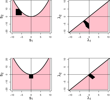
Figure 4: Left: Examples of rectangles ${\cal S}$ in terms of $(s_{1},s_{2})$. Right: Corresponding sets of eigenvalues $w^{-1}({\cal S})$.

The steps in the bootstrap, at a particular candidate mode $\widehat{m}_{j}$ (see Figure 5) are as follows (we suppress the subscript $j$):

1. Let $\widehat{\lambda}$ be the eigenvalues of the estimated Hessian and let $\widehat{s}=w(\widehat{\lambda})$.

2. Draw $Y_{1}^{*},\ldots,Y_{n}^{*}\sim P_{n}$ where $P_{n}$ is the empirical distribution of $Y_{1},\ldots,Y_{n}$.

3. Compute the density estimate, the Hessian and the estimates eigenvalues $\lambda^{*}=(\lambda_{1}^{*},\ldots,\lambda_{d}^{*})$. Compute the ESP-transformed eigenvalues $s^{*}=(s_{1}^{*},\ldots,s_{d}^{*})=w(\lambda^{*})$.

4. Repeat steps 2 and 3 $B$ times yielding $B$ vectors $s^{*1},\ldots,s^{*B}$.

5. Find the $1-\alpha/k$ bootstrap quantile $q$ defined by:

   $$\frac{1}{B}\sum_{b=1}^{B}I\Bigl{(}||s^{*b}-\widehat{s}||_{\infty}>q\Bigr{)}=\frac{\alpha}{k}.$$

   The set

   $${\cal S}=\Bigl{\{}s:\ ||s-\widehat{s}||_{\infty}\leq q\Bigr{\}}$$ (12)

   is a $1-\alpha$ asymptotic confidence set for $s=(s_{1},\ldots,s_{d})$.

6. Let

   $${\cal C}=\Biggl{[}\min_{b\in J}(-\lambda^{*b}_{1}),\ \ \max_{b\in J}(-\lambda^{*b}_{1})\Biggr{]}$$ (13)

   where $J=\Bigl{\{}1\leq b\leq B:\ s^{*b}\in{\cal S}\Bigr{\}}.$

The above procedure is used at each candidate mode $\widehat{m}_{j}$ and hence we get confidence sets ${\cal S}_{1},\ldots,{\cal S}_{k}$ for $s_{1},\ldots,s_{k}$, confidence rectangles $G_{1},\ldots,G_{k}$ for the $\gamma_{j}$’s and confidence intervals ${\cal C}_{1},\ldots,{\cal C}_{k}$ for $\gamma_{11},\ldots,\gamma_{1k}$. Here, $s_{j}=(s_{1j},\ldots,s_{dj})$ and $\gamma_{1j}$ is minus the largest eigenvalue of the Hessian at mode $\widehat{m}_{j}$.

The last two steps deserve some explanation. A confidence set for $\gamma_{1j}$ at $\widehat{m}_{j}$ is $w^{-1}({\cal S}_{j})$. From Corollary 1 of Beran and Srivastava (1985), it follows that

$$\liminf_{n\to\infty}\ \mathbb{P}(s_{j}\in{\cal S}_{j})\geq 1-\frac{\alpha}{k}$$

and hence

$$\liminf_{n\to\infty}\ \mathbb{P}(\gamma_{1j}\in w^{-1}({\cal S}_{j}))\geq 1-\frac{\alpha}{k}$$

Therefore,

$$\liminf_{n\to\infty}\ \mathbb{P}(\gamma_{1j}\in w^{-1}({\cal S}_{j})\ {\rm for\ each\ }j)\geq 1-\alpha.$$ (14)

We should point out that the result in Beran and Srivastava (1985) applies to covariance matrices. To adapt their results to the Hessian, we need a central limit theorem for the estimated Hessian. Such a result is provided by Theorem 3 of Duong et al. (2008) which shows that

$$\sqrt{n}|H|^{1/4}{\rm vech}\left[H^{1/2}\left(\widehat{\cal H}_{Y,h}-{\cal H}_{h}\right)H^{1/2}\right]\rightsquigarrow N(0,\Sigma_{2})$$ (15)

where $\Sigma_{2}=R({\rm vech}\nabla^{(2)}K)p_{h}(x)$, $R(g)=\int g(x)g^{T}(x)dx$.

Computing $w^{-1}({\cal S}_{j})$ exactly would require calculating the inverse map $w^{-1}$ explicitly. We do not know of any computationally efficient method for computing the inverse map $w$. However, we do know, by construction, that $\lambda^{*b}=w^{-1}(s^{*b})$ for each bootstrap sample. The set $\bigl{\{}w^{-1}(s^{*b}):\ s^{*b}\in{\cal S}_{j}\bigr{\}}$ approximates $w^{-1}({\cal S}_{j})$ arbitrarily well as $B\to\infty$. Thus, we can approximate $w^{-1}({\cal S}_{j})$ by ${\cal C}_{j}$ in step 6.

Local Mode Testing Algorithm 1. Split the data into two halves $X$ and $Y$. 2. Using $X$, construct $\widehat{p}_{X,h}$ and use the mean-shift algorithm to find the modes $\widehat{\cal M}=\{\widehat{m}_{1},\ldots\widehat{m}_{k}\}$ of $\widehat{p}_{X,h}$. 3. Using $Y$, find $\widehat{p}_{Y,h}$ and its gradient $\widehat{g}_{Y,h}$ and Hessian $\widehat{\cal H}_{Y,h}$. 4. For each candidate mode $m=\widehat{m}_{j}\in\widehat{\cal M}$: (a) Estimate the Hessian at $m$ and compute its eigenvalues $\widehat{\lambda}_{i}(m)$, $i=1,\ldots d.$ (b) Compute elementary symmetric polynomials $s_{i}(m)$, according to (4) for $i=1,\ldots,d$. (c) Generate $B$ bootstrap Hessians ${\cal H}^{*}_{b}(m)$, $b=1,\cdots,B$ and obtain $B$ corresponding elementary symmetrical polynomial $s_{i}^{*\,b}(m),i=1,\ldots d$. (d) Compute confidence rectangle $G_{j}$ and the confidence set ${\cal C}_{j}$. (e) Declare that there is a mode at $m=\widehat{m}_{j}$ if the confidence set ${\cal C}_{j}$ lies entirely above 0.

Figure 5: The Local Mode Testing Algorithm.

We automatically get confidence intervals for the $s^{\rm th}$ negative eigenvalue at the $j^{\rm th}$ mode $\gamma_{sj}$ where $s=1,\ldots,d$ and $j=1,\ldots,k$. Thus, in addition to the significance of the mode, we get valuable information about the shape of the mode, which we call the eigenportrait. This will be illustrated in Section 6.

5 Persistence

There is a completely different approach for eliminating non-significant modes based on the theory of persistent homology which has been the focus of recent research (Chazal et al. (2011); Edelsbrunner and Harer (2008)). We will not review persistent homology here but rather we describe the salient points that are germane to the present paper. The key ideas are from Chazal et al. (2011).

Consider a smooth density $p$ with $M=\sup_{x}p(x)<\infty$. The $t$-level set clusters are the connected components of the set $L_{t}=\{x:\ p(x)\geq t\}$. Suppose we find the upper level sets $L_{t}=\{x:\ p(x)\geq t\}$ as we vary $t$ from $M$ to $0$. Persistent homology measures how the topology of $L_{t}$ varies as we decrease $t$. In our case, we are only interested in the modes, which correspond to the zeroth order homology. (Higher order homology refers to holes, tunnels etc.)

Imagine setting $t=M$ and then gradually decreasing $t$. Whenever we hit a mode, a new level set cluster is born. As we decrease $t$ further, some clusters may merge and we say that one of the clusters (the one born most recently) has died. See Figure 6.

In summary, each mode $m_{j}$ has a death time and a birth time denoted by $(d_{j},b_{j})$. (Note that the birth time is larger than the death time because we start at high density and move to lower density.) The modes can be summarized with a persistence diagram where we plot the points $(d_{1},b_{1}),\ldots,(d_{k},b_{k})$ in the plane. See Figure 6. Points near the diagonal correspond to modes with short lifetimes. Chazal et al. (2011) suggested killing any mode with a short lifetime $\ell_{j}=b_{j}-d_{j}$. This requires choosing a significance threshold. Balakrishnan et al. (2013) suggest that this threshold can be based on the bootstrap quantile $\epsilon_{\alpha}$ defined by

$$\epsilon_{\alpha}=\inf\Biggl{\{}z:\ \frac{1}{B}\sum_{b=1}^{B}I\Bigl{(}||\widehat{p}_{h}^{*b}-\widehat{p}_{h}||_{\infty}>z\Bigr{)}\leq\alpha\Biggr{\}}.$$ (16)

Here, $\widehat{p}_{h}^{*b}$ is the density estimator based on the $b^{\rm th}$ bootstrap sample. This corresponds to killing a mode if it is in a $2\epsilon_{\alpha}$ band around the diagonal.

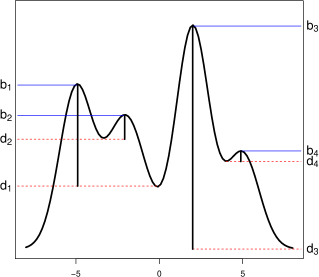
Figure 6: Starting at the top of the density and moving down, each mode has a birth time $b$ and a death time $d$. The persistence diagram (right) plots the points $(d_{1},b_{1}),\ldots,(d_{4},b_{4})$. Modes with a long lifetime are far from the diagonal.

The local test method proposed in this paper and the persistence method, each have advantages and disadvantages. The advantages of the persistence approach are that it does not require data-splitting, it does not require estimating derivatives and that, when used in its complete form, it can be used to find higher-order topological features. Also, the persistence diagram provides a simple visualization, independent of the dimension of the data.

The advantages of the local method are that it provides more shape information about each mode (via the confidence intervals for the eigenvalues of the Hessian) and that it is much faster since the bootstrap is only computed at $k$ points. In comparison, the bootstrap for the persistence approach has to be computed over a fine grid to approximate $||\widehat{p}_{h}^{*j}-\widehat{p}_{h}||_{\infty}$. Also, the local method never needs to compute the persistence of the modes which is itself computationally expensive.

In summary, there are advantages and disadvantages to each approach and in fact, they both provide useful information. The methods are less similar when one considers higher-order structure. The natural extension of local modes to higher-dimensional objects corresponds to ridges and hyper-ridges as in Genovese et al. (2013). In contrast, high-order persistent homology corresponds to holes and tunnels. Thus, the two approaches are aimed at different types of structure.

One thing that persistence and local eigenportraits have in common is that both permit visualization of data regardless of the dimension of the data.

6 Examples

We start with a few simple examples to illustrate the method. Figure 7 shows four one-dimensional examples. In each case $n=200$ and $\alpha=0.10$. The first column shows kernel density estimators and the second column shows confidence intervals for $\gamma_{1}$ at each mode.

The first two rows are based on data from a Normal distribution. Row 1 has a bandwidth of $h=1$ and we find one significant mode. In row 2 we use a small bandwidth namely $h=.1$. In this case there are numerous potential modes but each is declared to be non-significant as is evident from the plot of the confidence intervals for the $\gamma_{1j}$’s. This shows an important feature of our procedure: false modes that occur by using a bandwidth that is too small are correctly regarded as random fluctuations rather than being significant modes. This can be used as a diagnostic to alert us that the bandwidth is too small. We discuss this point further in Section 7. The next two rows show the results for a mixture of two Normals ($n=200$, $h=1$ and $\alpha=.10$) and a mixture of three Normals ($n=200$, $h=1.5$ and $\alpha=.10$). The method correctly finds the appropriate modes.

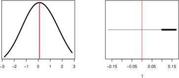
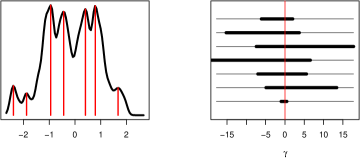
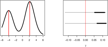
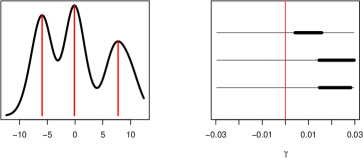
Figure 7: Left plots are kernel density estimators. Right plots are confidence intervals for the $\gamma_{1j}$’s. Top row: Normal data, $n=200$, $h=1$, $\alpha=0.10$. Second row: Normal data, $n=200$, $h=0.1$, $\alpha=0.10$. Third row: a mixture of two Normals, $n=200$, $h=1$ and $\alpha=.10$. Fourth row: a mixture of three Normals, $n=200$, $h=1$ and $\alpha=.10$.

The confidence intervals in Figure 8 are for a 10-dimensional dataset with two modes (a mixture of two Gaussians). The true density is $p(x)=\frac{1}{2}\phi(x;\mu_{1},\Sigma_{1})+\frac{1}{2}\phi(x;\mu_{2},\Sigma_{2})$ where

$$\mu_{1}=(-5,\ldots,-5),\ \ \ \mu_{2}=(5,\ldots,5),$$

$\Sigma_{1}$ is the identity matrix and $\Sigma_{2}$ is diagonal with diagonal entries $(1,1,1,1,1,.01,.01,.01,.01,.01)$. We used $n=10,000$, $h=1$ and $\alpha=0.05$. The procedure located four modes. The plots in Figure 8 are done per mode, rather than per eigenvalue. That is, there is one plot for each of the four modes, each showing the eigenportrait of all ten eigenvalues. We see that only two of the modes are significant. Thus two modes are correctly labeled as not real. The eigenportraits of the two significant modes are interesting. The first eigenportrait shows the spherical nature of the mode. The second shows that the mode is very non-spherical. Thus we have an informative way to visualize the 10-dimensional data.

Figure 9 shows a two-dimensional example with four modes that have different shapes. The eigenportrait reveals that one mode is highly non-spherical.

The data in Figure 10 show what happens when our assumptions are violated. The data have three well-separated modes. There is also a ring which, technically, consists of infinitely many, non-separated modes. Both the persistence method and the local testing method declare the three spherical modes to be significant. The modes on the ring are declared non-significant by both methods. The eigenportrait nicely distinguishes the difference in shape of the different modes.

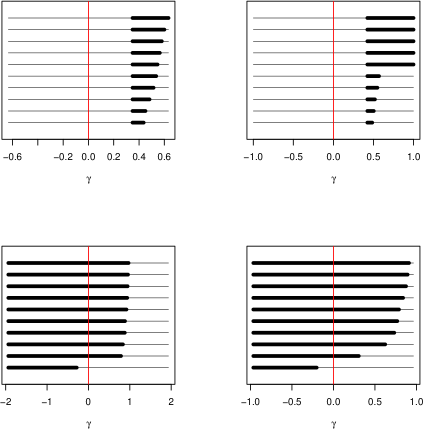
Figure 8: Eigenportrait of 10-dimensional data. Each plot shows confidence intervals for all 10 $\gamma_{j}$’s. The top two plots show the two significant modes. The bottom two plots show the two non-significant modes. Note that the eigenportraits of the significant modes show that the two modes have different shapes.

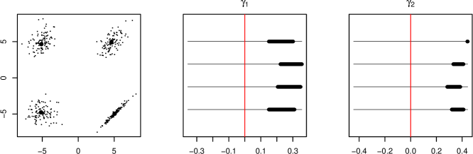
Figure 9: Left: Data with 4 modes of differing shapes. Middle: confidence intervals for $\gamma_{1j}$ at each mode. Right: confidence intervals for $\gamma_{2j}$ at each mode.

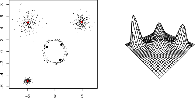
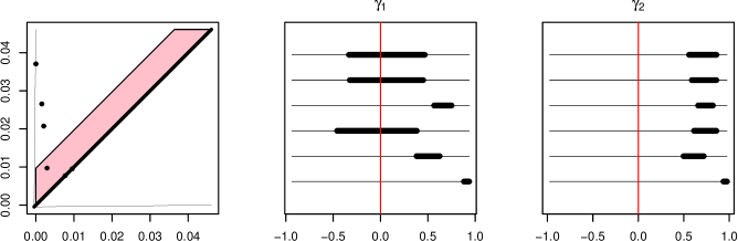
Figure 10: Top: 3 modes plus a ring. Bottom left: persistence diagram showing three significant modes and several non-significant modes. Points in the filled-in strip are declared to be non-significant. Middle: confidence intervals for $\gamma_{1}$ at each mode. (Three significant modes.) Right: confidence intervals for $\gamma_{2}$ at each mode.

Now we turn to the earthquake data analyzed in Duong et al. (2008). The data are the epicenters of 512 earthquakes before the 1982 eruption of Mt St Helens. The data, and the three significant modes we found are shown in Figure 11. The three variables are latitude, longitude and $-\log(-{\rm depth})$. We use a bandwidth of .3 (which is roughly consistent with the analysis in Duong et al. (2008).) Figure 12 shows the persistence diagram and the eigenportrait. All the analyses are consistent with three modes and three different depths. The modes we located are consistent with the regions of interest found in Duong et al. (2008). The eigenportraits show that $\gamma_{1}$ (corresponding to depth) has the most uncertainty (larger confidence intervals). This makes sense since the latitude and longitude have small variation.

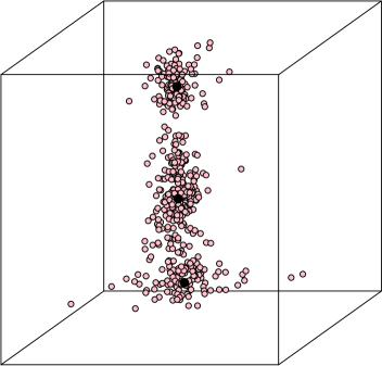
Figure 11: Scatterplot of the earthquake data. The three dark points are the estimated modes.

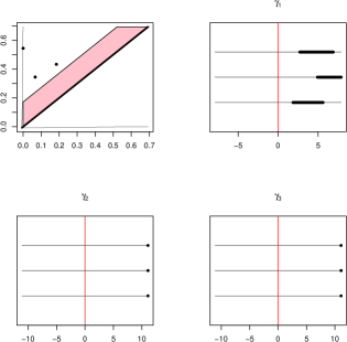
Figure 12: The earthquake data. Top left: the persistence diagram shows three significant modes. Points in the filled-in strip are declared to be non-significant. Top right: confidence intervals for $\gamma_{1}$. Bottom left: confidence intervals for $\gamma_{2}$. Bottom right: confidence intervals for $\gamma_{3}$.

7 A Possible Method For Choosing the Bandwidth

Bandwidth selection for mode hunting is a challenging problem. The first method we are aware of is Silverman (1981) although it has not been used much in practice. Recent, very promising work has focused on accurate estimation of derivatives; see Chacon and Duong (2013); Chacón and Monfort (2013). The results in this paper suggest another approach to selecting the bandwidth for mode hunting. The purpose of this section is to briefly (and heuristically) introduce the idea.

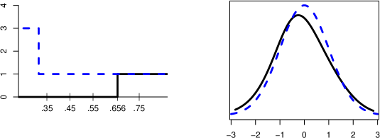
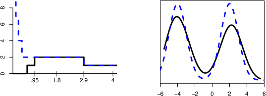
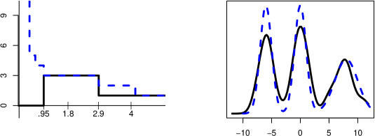
Figure 13: Left: Number of modes (dashed line) and number of significant modes (solid line) modes versus bandwidth. Right: true density (dashed) and estimated density (solid) using bandwidth $\widehat{h}$ given in equation (17).

We have seen that when the bandwidth $h$ is chosen to be small, many modes are found but our procedure identifies these modes as random fluctuations in the estimated density. On the other hand, when $h$ is large, there will be at most one mode.

Thus, while the number of modes decreases with $h$, the number of significant modes is small when $h$ is either too small or too large. If mode finding is our main goal, rather than accurate estimation in the $L_{2}$ norm, then this suggests a new way to choose the bandwidth $h$: choose $h$ to maximize the number of significant modes. More precisely, let $N(h)$ be the number of significant modes found by our test, as a function of $h$. Let $m=\max\{N(h):\ h>0\}$ and define

$$\widehat{h}=\inf\Bigl{\{}h:\ N(h)=m\Bigr{\}}.$$ (17)

We now examine the result of applying this procedure in a few examples. Figure 13 shows the number of modes and the number of significant modes $N(h)$ versus bandwidth for a Normal (top), a mixture of two Normals (middle) and a mixture of three Normals (bottom). In each case, choosing the bandwidth to maximize the number of significant modes leads to the correct number of modes.

Now we turn to a very challenging problem: selecting a bandwidth when the density is singular. Consider, for example, the distribution,

$$P=\frac{1}{3}N(-\mu,\sigma)+\frac{1}{3}\delta_{0}+\frac{1}{3}N(\mu,\sigma)$$

where $\delta_{0}$ is a point mass at 0. Of course, $P$ does not even have a density. Nonetheless, $p_{h}$ has three modes and a kernel density estimator will indeed show three modes for certain values of $h$. If we apply the usual cross-validation method, we will get $\widehat{h}=0$ because there are ties in the data. This leads to a useless estimator. What can we hope for in this example? Estimating well in the $L_{2}$ sense does not even make sense. Instead, we at least hope to get a density estimator with three modes. Figure 14 shows an example with $\mu=10$, $\sigma=1$ and $n=180$. Here we see that we do indeed get three modes.

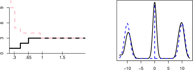
Figure 14: The true distribution is a mixture of two Normals and a point mass at 0. Left: number of modes (dashed) and number of significant modes (solid) versus bandwidth. Right: density estimator using $\widehat{h}$. The estimate is solid. The true density is dashed. We use a vertical line to indicate the singular component. The proposed bandwidth selection method chooses a bandwidth leading to a smooth density with three modes.

These results are very encouraging but, of course, a thorough investigation of the idea is needed before it can be recommended for general use. To establish theoretical properties of this method requires theory that is valid when $h\to 0$. Unfortunately, the usual asymptotic theory requires that $h^{d+4}n\to\infty$ which precludes small bandwidths. Hence, a rigorous theory for this method remains an open problem.

8 Theoretical Properties

We examine here some theoretical properties of the procedure described in Sections 3 and 4. Our main goal is to bound the width of the confidence interval for $\gamma_{1}$ (Theorem 5.) A secondary goal is to show that the modes discovered in stage 1 of the procedure are good estimators of the true modes. This fact has been established in various papers but we could not find an explicit statement of the result in the multivariate, multi-mode case so we include the details for completeness. We begin by restating the assumptions.

(A1) The density $p$ is a bounded, continuous density supported on a compact set ${\cal X}\subset\mathbb{R}^{d}$.

(A2) The gradient $g$ and Hessian ${\cal H}$ of $p$ are bounded and continuous. We assume that the Hessian is non-degenerate at every stationary point.

(A3) $p$ has finitely many modes $m_{1},\ldots,m_{k_{0}}$ in the interior of ${\cal X}$.

(A4) Let

$$\Delta=\min_{j\neq k}||m_{j}-m_{k}||\ \ \ \ \ \mbox{and}\ \ \ \ \ L=\max_{1\leq j\leq k_{0}}\lambda_{1}({\cal H}(m_{j})).$$ (18)

We assume that $\Delta>0$ and $L<0$.

(A5) The kernel $K$ is a symmetric probability density with bounded and continuous first and second derivatives and bounded second moment.

Properties of $p_{h}$. Recall that $\widehat{p}_{h}$ is the kernel density estimator with bandwidth matrix $H=h^{2}I$. Let $\widehat{g}_{h}$ and $\widehat{\cal H}_{h}$ are the gradient and Hessian of $\widehat{p}_{h}$. Let

$$p_{h}(x)=\int K(t)p(x+th)dt$$ (19)

be the mean of the kernel density estimator. Let $g_{h}$ and ${\cal H}_{h}$ denote the gradient and Hessian of $p_{h}$. For $h>0$ small enough, $p_{h}$ inherits all the above properties. The proofs of the following two lemmas are standard and are omitted.

Lemma 1

Assume (A1)-(A5). Assume that $h^{2}<C\epsilon$ for some $C$. Then, for all $h>0$ and $\epsilon$ small enough we have:

1. $p_{h}$ is a bounded and continuous density.

2. The gradient $g_{h}$ and Hessian ${\cal H}_{h}$ of $p_{h}$ are bounded and continuous.

3. $p_{h}$ has finitely many modes $m_{1h},\ldots,m_{k_{0}h}$ in the interior of ${\cal X}$ where $\max_{j}||m_{j}-m_{jh}||=O(h^{2})$.

4. $\Delta_{h}>0$ and $L_{h}<0$ where

   $$\Delta_{h}=\min_{j\neq k}||m_{jh}-m_{kh}||\ \ \ \ \ \mbox{and}\ \ \ \ \ L_{h}=\max_{1\leq j\leq k_{0}}\lambda_{1}({\cal H}_{h}(m_{jh})).$$

The conditions also guarantee that $p$ and $p_{h}$ are locally quadratic around their modes. Let $B(x,\epsilon)$ denote a ball of radius $\epsilon$ centered at $x$.

Lemma 2

Assume that $h^{2}<C\epsilon$ for some $C$. Let $B_{j}=B(m_{j},\epsilon)$. When $\epsilon$ and $h$ are small enough, $m_{jh}\in B_{j}$ for each $j$. Moreover, there exists $\delta>0$ and $c>0$ such that the following are true:

$$\max_{j}\sup_{x\in B_{j}}\lambda_{1}({\cal H}(x))\leq-\delta\ \ \ \mbox{and}\ \ \ \max_{j}\sup_{x\in B_{j}}\lambda_{1}({\cal H}_{h}(x))\leq-\delta$$

and, for all $j$ and all $x\in B_{j}$,

$$p(m_{j})-p(x)\geq c||x-m_{j}||^{2}\ \ \mbox{and}\ \ \ p_{h}(m_{jh})-p_{h}(x)\geq c||x-m_{jh}||^{2}.$$

Properties of $\widehat{p}_{h}$. Here we record some useful facts about $\widehat{p}_{h}$. We have that

$$\sup_{x\in{\cal X}}||\widehat{p}_{h}(x)-p_{h}(x)|| \leq C\sqrt{\frac{\log n}{nh^{d}}}$$

$$\sup_{x\in{\cal X}}||\widehat{g}_{h}(x)-g_{h}(x)|| \leq C\sqrt{\frac{\log n}{nh^{d+2}}}$$ (20)

$$\sup_{x\in{\cal X}}||\widehat{\cal H}_{h}(x)-{\cal H}_{h}(x)|| \leq C\sqrt{\frac{\log n}{nh^{d+4}}}$$

almost surely, for all large $n$. The first bound is proved in Giné and Guillou (2002) and the bounds on $\widehat{g}_{h}$ and $\widehat{\cal H}_{h}$ follow similarly. From Theorems 1 and 3 of Duong, Cowling, Koch and Wand (2008), we have that

$$\sqrt{nh^{d+2}}(\widehat{g}_{h}(x)-g_{h}(x))\rightsquigarrow N(0,\Sigma_{1})$$ (21)

where $\Sigma_{1}=p_{h}(x)\int\nabla K(x)\nabla K(x)^{T}dx$ and

$$\sqrt{nh^{d+4}}{\rm vech}(\widehat{\cal H}_{h}(x)-{\cal H}_{h}(x))\rightsquigarrow N(0,\Sigma_{2})$$ (22)

where $\Sigma_{2}=p_{h}(x)\int({\rm vech}\nabla^{(2)}K(x))({\rm vech}\nabla^{(2)}K(x))^{T}dx.$

Properties of the Estimated Modes. Let

$${\cal M} =\mbox{modes of}\ p$$

$${\cal M}_{h} =\mbox{modes of}\ p_{h}$$

$$\widehat{\cal M} =\mbox{modes of}\ \widehat{p}_{X,h}$$

$${\cal M}^{\dagger} =\mbox{modes in\ }\widehat{\cal M}\ \mbox{that pass the hypothesis test in Stage 2}.$$

Lemma 3

Let $\epsilon>0$ and $h>0$ be sufficiently small with $h^{2}<C\epsilon$ for some $C>0$. Let $B_{j}=B(m_{j},\epsilon)$. Let $B_{0}={\cal X}-\bigcup_{j=1}^{k}B_{j}$. Then, as $n\to\infty$:

1. $\mathbb{P}(B_{j}\bigcap\widehat{\cal M}\neq\emptyset\ {\rm for\ all\ }j)\to 1$. Thus, $\widehat{p}_{X,h}$ has at least one mode in each $B_{j}$.

2. With probability tending to 1, $\widehat{p}_{X,h}$ has exactly one mode $\widehat{m}_{jh}$ in each $B_{j}$.

3. Let $x_{n}$ be any maximizer of $\widehat{p}_{X,h}$ in $B_{j}$. Then

   $$||x_{n}-m_{jh}||=O_{P}\left((nh^{d})^{-1/4}\right)$$ (23)

   and

   $$||x_{n}-m_{j}||=O_{P}\left((nh^{d})^{-1/4}\right)+O(h^{2}).$$ (24)

Proof. (1) Since $\widehat{p}_{X,h}$ is a bounded continuous function, it has a maximizer over $B_{j}$. We claim that the maximizer must be in the interior of $B_{j}$. Write $B_{j}=A_{0}\cup A_{1}\cup A_{2}$ where $A_{0}=\{x:\ ||x-m_{j}||\leq\epsilon/3\}$, $A_{1}=\{x:\ \epsilon/3<||x-m_{j}||\leq 2\epsilon/3\}$ and $A_{2}=\{x:\ 2\epsilon/3<||x-m_{j}||\leq\epsilon\}$. For $C$ large enough, $m_{jh}\in A_{0}$. Also, from the properties of $p_{h}$,

$$\inf_{x\in A_{0}}p_{h}(x)>\sup_{x\in A_{2}}p_{h}(x).$$

With probability tending to 1,

$$\inf_{x\in A_{0}}\widehat{p}_{X,h}(x)\geq\inf_{x\in A_{0}}p_{h}(x)-C\sqrt{\frac{\log n}{nh^{d}}}>\sup_{x\in A_{2}}p_{h}(x)-C\sqrt{\frac{\log n}{nh^{d}}}\geq\sup_{x\in A_{2}}\widehat{p}_{X,h}(x)+C\sqrt{\frac{\log n}{nh^{d}}}.$$

So, with probability tending to 1,

$$\inf_{x\in A_{0}}\widehat{p}_{X,h}(x)>\sup_{x\in A_{2}}\widehat{p}_{X,h}(x).$$

This implies that any maximizer $x$ of $\widehat{p}_{X,h}$ over $B_{j}$ is in the interior of $B_{j}$ and hence $\widehat{g}_{X,h}(x)=(0,\ldots,0)^{T}$. Furthermore,

$$\lambda_{1}(\widehat{\cal H}_{X,h}(x))\leq\lambda_{1}({\cal H}_{X,h}(x))+o_{P}(1)\leq-\delta+o_{P}(1).$$

So, with probability tending to 1, $\widehat{p}_{X,h}$ has a maximizer $x$ in the interior of $B_{j}$ with 0 gradient and negative Hessian eigenvalues, i.e. it is a mode.

(2) Suppose $\widehat{p}_{X,h}$ has two modes $x$ and $y$ in $B_{j}$. So $\widehat{g}_{X,h}(x)=\widehat{g}_{X,h}(y)=(0,\ldots,0)^{T}$. Recall the exact Taylor expansion for a vector valued function $f$ is $f(a+t)-f(a)=t^{T}\int_{0}^{1}Df(a+ut)du.$ So

$$(0,\ldots,0)^{T}=\widehat{g}_{X,h}(y)-\widehat{g}_{X,h}(x)=(y-x)^{T}\int_{0}^{1}\widehat{\cal H}_{X,h}(x+u(y-x))du$$

and hence, multiplying on the right by by $y-x$,

$$0 =\int_{0}^{1}(y-x)^{T}\widehat{\cal H}_{X,h}(x+u(y-x))(y-x)du\leq||y-x||\sup_{u}\lambda_{1}(\widehat{\cal H}_{X,h}(x+u(y-x)))$$

$$\leq||y-x||\sup_{u}[\lambda_{1}({\cal H}_{X,h}(x+u(y-x)))+o_{P}(1)]$$

$$\leq||y-x||\Bigl{[}-\delta+o_{P}(1)\Bigr{]}<-\frac{\delta||y-x||}{2}$$

with probability tending to one. Hence, $x=y$.

(3) This proof uses a strategy similar to that in Donoho and Liu (1991, Theorem 5.5). Let $x$ be any maximizer of $\widehat{p}_{X,h}$ over $B_{j}$. Then $\widehat{p}_{X,h}(x)\geq\widehat{p}_{X,h}(m_{jh})$ (where $m_{jh}\in{\cal M}_{h}$) and hence

$$[\widehat{p}_{X,h}(x)-p_{h}(x)]-[\widehat{p}_{X,h}(m_{jh})-p_{h}(m_{jh})]\geq p_{h}(m_{jh})-p_{h}(x)\geq c||m_{jh}-x||^{2}$$

where we used Lemma 2. Hence,

$$Z_{n}(x)-Z_{n}(m_{jh})\geq c\sqrt{nh^{d}}||m_{jh}-x||^{2}$$

where $Z_{n}(x)=\sqrt{nh^{d}}(\widehat{p}_{X,h}(x)-p_{h}(x))$. It can be shown that $\sup_{x\in{\cal X}}||Z_{n}(x)||=O_{P}(1)$. Hence,

$$||m_{jh}-x||^{2}\leq\frac{1}{c\sqrt{nh^{d}}}\sup_{x}||Z_{n}(x)||=O_{P}\left(\sqrt{\frac{1}{nh^{d}}}\right).$$

Hence,

$$||x-m_{jh}||=O_{P}\left(\frac{1}{nh^{d}}\right)^{1/4}.$$ (25)

$\Box$

Properties of the ESP Transformation. By construction, the $1-\alpha$ asymptotic confidence set ${\cal S}$ in (12) is a $d$-dimensional hypercube in $\mbox{$\mathbb{R}$}^{d}$. The confidence interval ${\cal C}$ for $\lambda_{1}$ is

$$R=R({\cal S})=\Bigl{[}\inf\,\bigl{\{}a\in Q\bigr{\}},\ \ \sup\,\bigl{\{}a\in Q\bigr{\}}\Bigr{]}$$

where $Q=w^{-1}({\cal S})$. In this section, we bound the size of $R$.

Let ${\cal B}$ be the set of all symmetric $d\times d$ matrices and let ${\cal E}=\bigl{\{}w(\lambda(A)):\ A\in{\cal B}\bigr{\}}$. Thus, if $s=(s_{1},\ldots,s_{d})\in{\cal E}$ then $w^{-1}(s)$ corresponds to the eigenvalues of some symmetric matrix. Let ${\cal S}={\cal S}(s_{0},\epsilon)$ be any hyper-cube in $\mathbb{R}^{d}$:

$${\cal S}(s_{0},\epsilon)=\Bigl{\{}t\in\mathbb{R}^{d}:\ ||s-t||_{\infty}\leq\epsilon\Bigr{\}}$$

for some $s_{0}$ and $\epsilon$. We want to bound the size of

$$R=R({\cal S})=\Bigl{[}\inf\,\bigl{\{}a\in Q\bigr{\}},\ \ \sup\,\bigl{\{}a\in Q\bigr{\}}\Bigr{]}$$

where $Q=w^{-1}({\cal S}\bigcap{\cal E})$.

Each $s\in{\cal S}\cap{\cal E}$ defines a characteristic polynomial

$$P_{s}(\lambda)=\prod_{i=1}^{d}(\lambda_{i}-\lambda)=\lambda^{d}+\sum_{k=1}^{d}(-1)^{k}\ s_{k}\ \lambda^{d-k}=0$$ (26)

whose roots are the eigenvalues of some symmetric matrix.

Lemma 4

There exists $C>0$, depending only $\epsilon_{0}$ and $s_{0}$, such that, for all $\epsilon<\epsilon_{0}$,

$$C\epsilon+o(\epsilon)\leq\mu(R({\cal S}(s_{0},\epsilon)\cap{\cal E}))\leq C\epsilon^{1/d}.$$

Proof. Without loss of generality, assume that $d$ is even. (A simple modification of the proof works for $d$ odd.) First, note that, there is some $L>0$ (depending on $s_{0}$ and $\epsilon_{0}$) such that for all $\epsilon<\epsilon_{0}$ and all $s\in{\cal S}(s,\epsilon)$, we have $-L\leq\lambda_{d}(s)\leq\lambda_{1}(s)\leq L$. Let $s,\widetilde{s}\in{\cal S}\bigcap{\cal E}$ so that $||\widetilde{s}-s_{0}||_{\infty}\leq 2\sqrt{d}\epsilon$. Let $P_{s}$ and $\widetilde{P}_{\widetilde{s}}$ be the polynomials corresponding to $s$ and $\widetilde{s}$. Then

$$|P_{s}(\lambda)-\widetilde{P}_{\widetilde{s}}\ (\lambda)|\leq\sum_{k=1}^{d}|(-1)^{k}|\ |s_{k}-\widetilde{s}_{k}|\ |\lambda^{d-k}|\leq\ 2\sqrt{d}\ \epsilon\sum_{k=1}^{d}|\lambda|^{d-k}\ \leq\ C\ \epsilon$$ (27)

where $C=2\sqrt{d}\sum_{k=1}^{d}L^{d-k}$. Let $\lambda$ and $\widetilde{\lambda}$ be the ordered eigenvalues of $P_{s}$ and $\widetilde{P}_{\widetilde{s}}$. First, suppose $\widetilde{\lambda}_{1}>\lambda_{1}$. For all $\lambda>\lambda_{1}$, the polynomial in (26) can be written as $P_{s}(\lambda)=\prod_{i=1}^{d}(\lambda-\lambda_{i})$ showing that it is an increasing function of $\lambda$, since each factor in the product is increasing. Let $\lambda_{1}<t<\widetilde{\lambda}_{1}$, then

$$P_{s}\,(\widetilde{\lambda}_{1})=\prod_{i=1}^{d}(\widetilde{\lambda}_{1}-\lambda_{i})\geq(\widetilde{\lambda}_{1}-\lambda_{1})^{d}.$$

From (27)

$$C\ \epsilon\ \geq|P_{s}(\widetilde{\lambda}_{1})-\widetilde{P}_{\widetilde{s}}\ (\widetilde{\lambda}_{1})|\ =\ |P_{s}(\widetilde{\lambda}_{1})|\ \geq\ \ (\widetilde{\lambda}_{1}-\lambda_{1})^{d}.$$

Hence, $\lambda_{1}\leq\widetilde{\lambda}_{1}\leq(C\epsilon)^{1/d}$. Now assume $\widetilde{\lambda}_{1}<\lambda_{1}$. Then

$$\widetilde{P}_{\widetilde{s}}\ (\lambda_{1})=\prod_{i=1}^{d}(\lambda_{1}-\widetilde{\lambda}_{i})\geq(\lambda_{1}-\widetilde{\lambda}_{1})^{d}.$$

Similarly, from (27)

$$C\ \epsilon\ \geq|P_{s}(\lambda_{1})-\widetilde{P}_{\widetilde{s}}(\lambda_{1})|\ =\ |\widetilde{P}_{\widetilde{s}}(\lambda_{1})|\ \geq\ |\widetilde{\lambda}_{1}-\lambda_{1}|^{d}.$$

Thus $|\widetilde{\lambda}_{1}-\lambda_{1}|<C\ \epsilon^{1/d}$. The lower bound follows by choosing some point $s\in{\cal S}(s_{0},\epsilon)\cap{\cal E}$ that is in the interior of ${\cal E}$. For such a point, $\lambda$ is a continuously differentiable function of $s$ and the bound follows from a simple Taylor expansion. $\Box$

Remark: The worst case is when $\lambda_{1}=\cdots=\lambda_{d}$ and the characteristic polynomial is simply $(\lambda_{1}-\lambda)^{d}$. In that case, a small perturbation of $s$ can cause a perturbation of $\lambda_{1}$ of size $O(\epsilon^{1/d})$.

Properties of the Confidence Interval and Test.

Theorem 5

Let ${\cal C}_{j}$ be the confidence interval for $\gamma_{1j}=-\lambda_{1}({\cal H}_{h}(x))$ for any $x$. Then the Lebesgue measure is

$$\mu({\cal C}_{j})=O_{P}\left((nh^{d+4})^{-1/d}\right).$$

Proof Outline. We can write $s=f({\cal H}_{h})$ for some smooth, continuously differentiable function $f$. The asymptotic variance of $\widehat{\cal H}_{Y,h}$ is of order $\epsilon_{n}$ where $\epsilon_{n}=O_{P}((nh^{d+4})^{1/2})$. It may then be shown that the $1-\alpha$ confidence rectangle for $s$ has size of order $\epsilon_{n}$. The result then follows From Lemma 4, the size of of ${\cal C}_{j}$ is $O(\epsilon_{n}^{1/d})$. $\Box$

Lemma 6

Let $B_{j}=B(m_{j},\epsilon)$. We have:

1. $\mathbb{P}(B_{j}\cap{\cal M}^{\dagger}\neq\emptyset\ {\rm for\ all\ }j)\to 1$.

2. Let $B_{0}=\{x:\ \lambda_{1}({\cal H}_{h}(x))\geq 0\}$. Then $\limsup_{n\to\infty}\mathbb{P}(\widehat{\cal M}^{\dagger}\cap B_{0}\neq\emptyset)\leq\alpha$.

Proof. (1) In parts (1) and (2) of Lemma 3 we showed there exists one mode $\widehat{m}_{jh}\in B_{j}$ with zero gradient and negative eigenvalues. In Theorem 5, we showed that the width of the confidence interval for the first eigenvalue of the Hessian at $\widehat{m}_{jh}$ shrinks to 0. This implies that, with probability tending to 1, the test rejects the null and hence $\widehat{m}_{jh}$ is included in ${\cal M}^{\dagger}$.

(2) Let $x\in B_{0}$. Then $x\in{\cal M}^{\dagger}$ if and only if $x\in\widehat{\cal M}$ and if the confidence interval excludes the true value of $\lambda_{1}({\cal H}_{h}(x))$. Let $U=\widehat{\cal M}\cap B_{0}$. Conditional on $X$, the probability that the test rejects the null for any $z\in Z$ has, asymptotically, probability at most $\alpha/k$. Hence, $\mathbb{P}(U\neq\emptyset|X)\leq\alpha+o(1)$ and, by the independence of $X$ and $Y$, $\mathbb{P}(U\neq\emptyset)\leq\alpha+o(1)$. $\Box$

When the Bandwidth is Small. When $h$ is small, we get spurious modes which are killed off by the hypothesis test. This behavior is clear in the examples. Intuitively, it follows since the size of confidence rectangle increases as $h$ decreases. We have seen numerically that this prevents us from choosing a bandwidth that is too small because the number of significant modes becomes 0 when $h$ is too small. Making this fact rigorous remains an open question. When $h$ gets very small, the usual asymptotic methods no longer apply. It is possible that uniform-in-bandwidth asymptotics (Einmahl and Mason (2005)) might be useful here but this is beyond the scope of the paper and we leave this to future work.

9 Discussion

We have introduced a new method for testing the significance of modes in density estimators. There are several ideas that we hope to deal with in future work. These include the following:

1. Our method complements the approaches in Duong et al. (2008) and Chazal et al. (2011) by providing extra information about the estimated modes. A thorough investigation into combining the strengths of all three methods deserves future work.

2. If one makes specific assumptions about the size and separation of the modes, then it should be possible to find the asymptotic power of the test.

3. We indicated a possible method for choosing the bandwidth for mode hunting. Deriving precise theoretical properties of the method will require techniques that allow small bandwidths.

4. The ultimate goal of this line of work is to show that the clusters based on the significant modes are a good approximation to the population clusters ${\cal A}_{1},\ldots,{\cal A}_{k_{0}}$ defined in (4). The results in this paper are only a first step towards that goal. We would like to show, in fact, that with high probability, ${\cal A}_{j}$ contains one and only one significant mode. Furthermore, Chacón (2012) suggest an interesting risk function for mode clustering. We conjecture that deleting non-significant modes before clustering may improve the risk of mode-based clustering. Also, we conjecture that our bandwidth selection method will lead to good clustering risk.

References

- Arias-Castro et al. (2013) Ery Arias-Castro, David Mason, and Bruno Pelletier. On the estimation of the gradient lines of a density and the consistency of the mean-shift algorithm. Unpublished Manuscript, 2013.
- Balakrishnan et al. (2013) Sivaraman Balakrishnan, Brittany Fasy, Fabrizio Lecci, Alessandro Rinaldo, Aarti Singh, and Larry Wasserman. Statistical inference for persistent homology. arXiv preprint arXiv:1303.7117, 2013.
- Beran and Srivastava (1985) Rudolf Beran and Muni S Srivastava. Bootstrap tests and confidence regions for functions of a covariance matrix. The Annals of Statistics, pages 95–115, 1985.
- Cadre (2006) B. Cadre. Kernel estimation of density level sets. Journal of multivariate analysis, 97(4):999–1023, 2006.
- Chacón (2012) Chacón. Clusters and water flows: a novel approach to modal clustering through morse theory. arXiv preprint arXiv:1212.1384, 2012.
- Chacón and Monfort (2013) J. Chacón and P. Monfort. A comparison of bandwidth selectors for mean shift clustering. arXiv preprint arXiv:1310.7855, 2013.
- Chacón and Duong (2010) JE Chacón and T. Duong. Multivariate plug-in bandwidth selection with unconstrained pilot bandwidth matrices. Test, 19(2):375–398, 2010.
- Chacón et al. (2011) J.E. Chacón, T. Duong, and MP Wand. Asymptotics for general multivariate kernel density derivative estimators. Statistica Sinica, 21:807–840, 2011.
- Chacon and Duong (2013) Jose Chacon and Tarn Duong. Data-driven density derivative estimation, with applications to nonparametric clustering and bump hunting. Electronic Journal of Statistics, 7:1935–2524, 2013.
- Chazal et al. (2011) F. Chazal, L.J. Guibas, S.Y. Oudot, and P. Skraba. Persistence-based clustering in riemannian manifolds. In Proceedings of the 27th annual ACM symposium on Computational geometry, pages 97–106. ACM, 2011.
- Comaniciu and Meer (2002) D. Comaniciu and P. Meer. Mean shift: a robust approach toward feature space analysis. Pattern Analysis and Machine Intelligence, IEEE Transactions on, 24(5):603 –619, may 2002. ISSN 0162-8828. doi: 10.1109/34.1000236.
- Donoho and Liu (1991) David L Donoho and Richard C Liu. Geometrizing rates of convergence, iii. The Annals of Statistics, pages 668–701, 1991.
- Dümbgen and Walther (2008) L. Dümbgen and G. Walther. Multiscale inference about a density. The Annals of Statistics, 36(4):1758–1785, 2008.
- Duong et al. (2008) Tarn Duong, Arianna Cowling, Inge Koch, and MP Wand. Feature significance for multivariate kernel density estimation. Computational Statistics & Data Analysis, 52(9):4225–4242, 2008.
- Edelsbrunner and Harer (2008) Herbert Edelsbrunner and John Harer. Persistent homology-a survey. Contemporary mathematics, 453:257–282, 2008.
- Einmahl and Mason (2005) Uwe Einmahl and David M Mason. Uniform in bandwidth consistency of kernel-type function estimators. The Annals of Statistics, 33(3):1380–1403, 2005.
- Fukunaga and Hostetler (1975) Keinosuke Fukunaga and Larry D. Hostetler. The estimation of the gradient of a density function, with applications in pattern recognition. IEEE Transactions on Information Theory, 21:32–40, 1975.
- Genovese et al. (2013) Christopher R. Genovese, Marco Perone-Pacifico, Isabella Verdinelli, and Larry Wasserman. Nonparametric ridge estimation. arXiv preprint arXiv:1212.5156v1, 2013.
- Giné and Guillou (2002) E. Giné and A. Guillou. Rates of strong uniform consistency for multivariate kernel density estimators. In Annales de l’Institut Henri Poincare (B) Probability and Statistics, volume 38, pages 907–921. Elsevier, 2002.
- Godtliebsen et al. (2002) F Godtliebsen, JS Marron, and Probal Chaudhuri. Significance in scale space for bivariate density estimation. Journal of Computational and Graphical Statistics, 11(1):1–21, 2002.
- Klemelä (2005) J. Klemelä. Adaptive estimation of the mode of a multivariate density. Journal of Nonparametric Statistics, 17(1):83–105, 2005.
- Klemelä (2009) J. Klemelä. Smoothing of Multivariate Data: Density Estimation and Visualization. Wiley, 2009.
- Konakov (1974) VD Konakov. On the asymptotic normality of the mode of multidimensional distributions. Theory of Probability & Its Applications, 18(4):794–799, 1974.
- Li et al. (2007) J. Li, S. Ray, and B.G. Lindsay. A nonparametric statistical approach to clustering via mode identification. Journal of Machine Learning Research, 8(8):1687–1723, 2007.
- Mammen et al. (1992) Enno Mammen, James S Marron, and Nick I Fisher. Some asymptotics for multimodality tests based on kernel density estimates. Probability Theory and Related Fields, 91(1):115–132, 1992.
- Matsumoto (2002) Y. Matsumoto. An Introduction to Morse Theory. American Mathematical Society, 2002.
- Müller and Sawitzki (1991) Dietrich Werner Müller and Günther Sawitzki. Excess mass estimates and tests for multimodality. Journal of the American Statistical Association, 86(415):738–746, 1991.
- Polonik (1995) W. Polonik. Measuring mass concentrations and estimating density contour clusters-an excess mass approach. The Annals of Statistics, pages 855–881, 1995.
- Silverman (1981) Bernard W Silverman. Using kernel density estimates to investigate multimodality. Journal of the Royal Statistical Society. Series B (Methodological), pages 97–99, 1981.
- Walther (1997) G. Walther. Granulometric smoothing. The Annals of Statistics, pages 2273–2299, 1997.