Regular and exceptional spectra of the two-qubit quantum Rabi model

Abstract

We have studied the two-qubit quantum Rabi model in the asymmetric case and its generalizations with dipole and Heisenberg-type qubit-qubit interactions. The solutions are obtained analytically with eigenstates given in terms of the extended coherent states. These models are relevant to the construction of ultrafast two-qubit quantum gates and quantum state storage. For identical qubit-photon couplings, a novel type of quasi-exact solution which exists for all coupling values with constant eigenenergy is found, leading to level crossings within the same parity subspace even for non-identical qubits. In contrast to the quasi-exact states of the single-qubit model, the condition for these exceptional eigenstates depends only on a fine-tuning of the qubit level splittings but not on the coupling to the photon field. This makes them excellent candidates for direct experimental observation within circuit QED.

I Introduction

The quantum Rabi model jc describes in a very simple way the interaction between light and matter, the latter being modeled by a single spin-$1/2$ particle. It has found wide application in quantum optics guo ; tw , circuit QED sola ; tk , cavity QED s ; ac ; ih and quantum information aj . Theoretically, various investigations have been undertaken to solve it schweb ; swa ; trave ; vv . An analytical solution was obtained in br , using the Bargmann space of entire functions to model the bosonic degree of freedom barg . At the same time, developments in the field of circuit QED have reached the ultrastrong qubit-photon coupling region so ; so1 . Ensuing work studied other aspects of the full Rabi Hamiltonian, such as real-time dynamics and dynamical correlation functions bra1 ; bra2a , new methods to rederive the solution of the same model ly ; qing ; braak , and several generalizations trav ; pj ; 2bite ; pj1 ; bra2 ; dicke .

An important generalization of the single-qubit case, the two-qubit system with various interactions cpl is the simplest model of the universal quantum gate jj ; cp and has therefore applications in quantum state storage and transfer cp1 ; jm . The general two-qubit Rabi model has to be described for values of the coupling in the ultrastrong and deep strong regime where the rotating-wave approximation breaks down so , to be relevant to the recent developments in quantum optics ag ; jlf ; zrhk and quantum information afe ; rg .

In this paper, we will give its solution for the case of discernible qubits analytically, using a generalization of the method used in br , and also with extended coherent state method qing . At the same time, we consider some types of qubit-qubit interactions based on this model, including dipole interaction suda ; ggc , XXX fa and XYZ aa ; gs Heisenberg interactions. These generalized models allow for additional control of the system and may thus be of interest for applications. The eigenstates are obtained in terms of extended coherent states or Fock states. These expansions form the natural basis for numerical studies of the real-time evolution, unbiased by the truncation procedure bra1 . For identical qubit-photon couplings, there exists a novel type of quasi-exact solution for all the coupling values $g$ with constant eigenenergy, and the condition for its existence just depends on the qubit energy splittings if the qubit-qubit interactions are not taken into consideration. In contrast to the single-qubit case, these exceptional eigenstates have finite photon number and may be easily accessible in experiments, giving them possible application in quantum computation. A well-known example of these states are the spin-singlet “dark” states rod-lara for identical qubits, corresponding to a decoupling of the singlet sector. Remarkably, they exist also if the permutation symmetry is partially broken and the qubits are strongly coupled to the radiation field. If the qubits do not interact, we have found one such state for non-identical qubits. For a special choice of interaction, two exceptional states of the novel type are present in the spectrum.

Although all considered models possess a $\mathbb{Z}_{2}$-symmetry, this discrete symmetry is not sufficient to render them integrable because the dimension of the spin space (four) exceeds the number (two) of irreducible representations of $\mathbb{Z}_{2}$, according to the labeling criterion for quantum integrability introduced in br .

The paper is organized as follows. In Sec. II, we obtain the regular spectrum and the exceptional solutions of the two-qubit quantum Rabi model using Bargmann-space techniques and extended coherent state method. The exceptional solutions are given in closed form. In Sec. III, we generalize the two-qubit quantum Rabi model to include the dipole, XXX, and XYZ Heisenberg interactions and obtain their regular and exceptional solutions. Finally, we draw some conclusions including perspectives for future work in Sec. IV.

II Solution of the two-qubit quantum Rabi model

A Regular spectrum of the two-qubit quantum Rabi model

The Hamiltonian of the asymmetric two-qubit quantum Rabi model reads ($\hbar=1$)

$$H_{tq}= \omega a^{\dagger}a+g_{1}\sigma_{1x}(a+a^{\dagger})+g_{2}\sigma_{2x}(a+a^{\dagger})$$

$$+\Delta_{1}\sigma_{1z}+\Delta_{2}\sigma_{2z},$$ (1)

where $a^{\dagger}$ and $a$ are the single mode photon creation and annihilation operators with frequency $\omega$, respectively, and $\sigma_{i}\,(i=x,y,z)$ are the Pauli matrices. $2\Delta_{1}$, $2\Delta_{2}$ are the transition frequencies of the two (discernible) qubits. $g_{1}$ and $g_{2}$ are the qubit-photon coupling constants for the two qubits respectively. (The fully symmetric case corresponds to $g_{1}=g_{2}$, $\Delta_{1}=\Delta_{2}$.) First we make unitary transformations to interchange $\sigma_{x}$ and $\sigma_{z}$ and obtain $H^{\prime}_{tq}$. In Fock space, this Hamiltonian is infinite dimensional with off-diagonal elements. However, by using its $\mathbb{Z}_{2}$ symmetry with the transformation $R^{\prime}=R\otimes\sigma_{1x}\otimes\sigma_{2x}$, where $R=\exp(i\pi a^{\dagger}a)$, we obtain its solution analytically in the Bargmann space br ; barg , in which the bosonic creation and annihilation operators have the realizations $a~{}\rightarrow~{}\frac{\partial}{\partial z}$, $a^{\dagger}~{}\rightarrow~{}z$, with $z$ being a complex variable.

Setting $\omega=1$ and following the same procedure as pj , we obtain after a Fulton-Gouterman transformation $U$ fg ; pj , $U^{\dagger}H^{\prime}_{tq}U=\left(\begin{array}[]{cc}H_{+}&0\\ 0&H_{-}\\ \end{array}\right)$, where

$$H_{\pm}=z\partial_{z}+g_{1}(z+\partial_{z})+g_{2}(z+\partial_{z})\sigma_{2z}$$

$$+\Delta_{2}\sigma_{2x}\pm\Delta_{1}R\sigma_{2x},$$ (2)

acting on the subspace where $R^{\prime}$ has eigenvalues $\pm 1$ respectively. We expand $H_{\pm}$ in the basis of $\{|e\rangle\otimes\varphi^{\pm}_{1}$, $|g\rangle\otimes\varphi^{\pm}_{2}\}$, where $\varphi^{\pm}_{1}$ and $\varphi^{\pm}_{2}$ are photon field wavefunctions. Making the transformation $z\rightarrow-z$ to utilize the reflection symmetry and denoting $\varphi_{3}(z)=\varphi_{1}(-z)$, $\varphi_{4}(z)=\varphi_{2}(-z)$, we reduce the eigenvalue problem to four coupled differential equations (see Eqs. (27)–(30) in Appendix A). $\varphi^{\pm}_{j}$ ($j=1,\ldots,4$) can be expanded into normalized extended coherent states

$$|n,-\alpha\rangle=\frac{e^{-\alpha^{2}/2+\alpha z}}{\sqrt{n!}}(z-\alpha)^{n}$$ (3)

as $\varphi^{\pm}_{j}=e^{\alpha^{2}/2}\sum_{n=0}^{\infty}\sqrt{n!}e^{\pm}_{j,n}|n,-\alpha\rangle$, where $\alpha$ is a complex variable, with the recurrence relations of $e^{\pm}_{j,n}$ as Eqs. (31)–(34) in Appendix A.

Here the continued-fraction techniques, which work for the one-qubit case, fail for $g_{1}\neq g_{2}$, because the equivalent recurrence relation for $e^{\pm}_{1,n}$ has more than three terms if the $e^{\pm}_{2,n}\ldots e^{\pm}_{4,n}$ are eliminated. However, we can utilize the analyticity property of the Bargmann space br ; barg . All the power series depend on four free initial conditions $e^{\pm}_{j,0}$. Every expansion has a certain radius of convergence $R_{\alpha}$, and we choose $|z-\alpha|<R_{\alpha}$ so that the power series are absolutely convergent and a finite number of terms suffices to compute the function reliably. In contrast to numerical calculations in a truncated Hilbert space, where convergence is found “empirically”, convergence is a known property in our scheme. Analyticity requires the wavefunctions in the overlap of expansions around different points $\alpha$, $\alpha^{\prime}$ to be the same, which furnishes four equations $\varphi^{\pm}_{j}(z_{0})=\varphi^{\prime\pm}_{j}(z_{0})$ at a point $z_{0}$ in the overlap bra2 . But there are eight free initial conditions, so this will not impose enough constraints to obtain the eigenvalue $E$ if $\alpha$, $\alpha^{\prime}$ are arbitrary ordinary points of Eqs. (27) – (30). However, by analyzing the structure of the recurrence relations for $e^{\pm}_{j,n}$ and considering $\varphi^{\pm}_{1}(z)=\varphi^{\pm}_{3}(-z)$, $\varphi^{\pm}_{2}(z)=\varphi^{\pm}_{4}(-z)$ at $z=0$, we find for some special cases: $\alpha=\pm g$, $\pm g^{\prime}$, $0$, the free initial conditions reduce to less than four. Choosing $\alpha=0$, $g^{\prime}$ and $g$, we denote $\varphi^{\pm}_{j}(z)$ by $\Phi^{\pm}_{j}(z)$, $\phi^{\pm}_{j}(z)$ and $\psi^{\pm}_{j}(z)$, respectively. The corresponding radii of convergence are $R_{\alpha=0}=g^{\prime}$, $R_{\alpha=g^{\prime}}=\min\{2g^{\prime},g-g^{\prime}\}$, $R_{\alpha=g}=g-g^{\prime}$. The singularity structure for $\varphi^{\pm}_{j}$ in the complex plane is shown in Fig. 1.

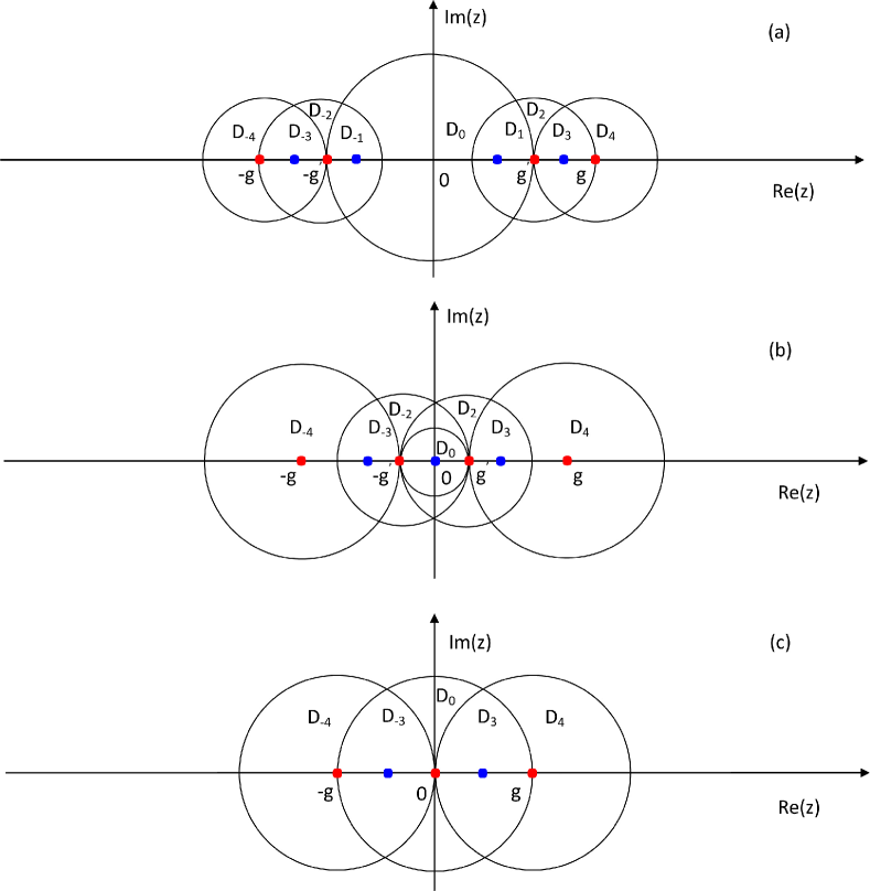
FIG. 1: (Color online) The singularity structure of $\varphi^{\pm}_{j}$ in the complex plane, where $D_{0}$, $D_{\pm 2}$ and $D_{\pm 4}$ denote the circles of convergence of $\varphi^{\pm}_{j}$ expanded around $0$, $\pm g^{\prime}$ and $\pm g$ respectively. Red/Light grey points denote regular singular points, while blue/dark grey ones are ordinary points. (a) $g^{\prime}\geq g/2$. $D_{\pm 1}=D_{0}\cap D_{\pm 2}$ and $D_{\pm 3}=D_{\pm 2}\cap D_{\pm 4}$ are the corresponding overlaps. (b) $0<g^{\prime}\leq g/3$. $D_{\pm 3}=D_{\pm 2}\cap D_{\pm 4}$. (c) $g^{\prime}=0$. $D_{\pm 3}=D_{0}\cap D_{\pm 4}$.

Now there are eight free initial conditions $\{e^{\pm,\alpha=0}_{1,0},$ $e^{\pm,\alpha=0}_{2,0}$, $e^{\pm,\alpha=g^{\prime}}_{1,0}$, $e^{\pm,\alpha=g^{\prime}}_{2,0}$, $e^{\pm,\alpha=g^{\prime}}_{3,0}$, $e^{\pm,\alpha=g}_{1,0}$,  $e^{\pm,\alpha=g}_{2,0}$, $e^{\pm,\alpha=g}_{4,0}\}$, determined by the following eight equations

$$\Phi^{\pm}_{j}(z_{0}^{\prime})-\phi^{\pm}_{j}(z_{0}^{\prime})=0,~{}\phi^{\pm}_{j}(z_{0})-\psi^{\pm}_{j}(z_{0})=0,$$ (4)

where $z_{0}^{\prime}$ and $z_{0}$ are arbitrary points which satisfy $|z-\alpha|<R_{\alpha}$, with which the analyticity condition of the Bargmann space in the whole complex plane is fulfilled. The condition for the linear equations (4) to have non-trivial solutions reads $G_{\pm}=\det(M_{\pm})=0$ for the $8*8$ coefficient matrix $M_{\pm}$ of Eq. (4) (see Eq. (51) in Appendix A), which can be used to determine the eigenvalue $E$ and sequently the eigenfunction $\varphi^{\pm}_{j}$ for $\alpha=0$, $g^{\prime}$, $g$. For $g^{\prime}=0.6g$, we choose $z_{0}=(g^{\prime}+g)/2$ in $D_{2}$ and $z^{\prime}_{0}=(g^{\prime})^{2}/g$ in $D_{1}$, which satisfies $z^{\prime}_{0}/g^{\prime}=(g^{\prime}-z^{\prime}_{0})/(g-g^{\prime})$ and obtain $G_{\pm}$, shown in Fig. 2. The eigenenergy locates at the zero of $G_{\pm}$, which does not vary with different $z_{0}$ and $z_{0}^{\prime}$.

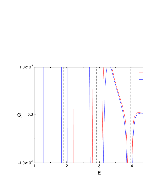
FIG. 2: The G-function of two-qubit Rabi model with $\Delta_{1}=0.6$, $\Delta_{2}=0.2$, $\omega=1$, $g=0.3$, $g^{\prime}=0.18$. Blue lines denote $G_{-}$ and red lines denote $G_{+}$, while dashed vertical lines are base lines.

For $0<g^{\prime}<g/2$, as shown in Fig. 1(b), one can choose $z_{0}^{\prime}=0$, then since $\Phi_{1}(0)=\Phi_{3}(0)=e^{\prime\prime}_{1,0}$ and $\Phi_{2}(0)=\Phi_{4}(0)=e^{\prime\prime}_{2,0}$, one finds $\phi_{j}(0)=\Phi_{j}(0)$ is equivalent to $\phi_{3}(0)=\phi_{1}(0)$, $\phi_{4}(0)=\phi_{2}(0)$, and the matrix can be reduced to $6$ dimensions.

For a special case $g^{\prime}=0$, i.e. $g_{1}=g_{2}$, we only need to choose $\alpha=0$ and $g$ (see Fig. 1(c)), and there are four equations

$$\Phi^{\pm}_{j}(z_{0})=\psi^{\pm}_{j}(z_{0})$$ (5)

for four free initial conditions $\{e^{\pm,\alpha=0}_{1,0}$, $e^{\pm,\alpha=g}_{1,0}$, $e^{\pm,\alpha=g}_{2,0}$, $e^{\pm,\alpha=g}_{4,0}\}$. The lowest part of the spectra for four sets of parameters are shown in Fig. 2, coinciding with the numerical results very well. The total wave function can be obtained as

$$\chi^{\pm}= e^{\alpha^{2}/2}\sum_{n=0}^{\infty}\sqrt{\frac{n!}{2}}[e^{\pm}_{1,n}\frac{1\pm R}{2}|n,-\alpha\rangle(|e,e\rangle+|g,g\rangle)$$

$$+e^{\pm}_{1,n}\frac{1\mp R}{2}|n,-\alpha\rangle(|e,g\rangle+|g,e\rangle)$$

$$+e^{\pm}_{2,n}\frac{1\pm R}{2}|n,-\alpha\rangle(|e,e\rangle-|g,g\rangle)$$

$$+e^{\pm}_{2,n}\frac{1\mp R}{2}|n,-\alpha\rangle(|g,e\rangle-|e,g\rangle)].$$ (6)

For $\alpha=0$, one has

$$\chi^{\pm}= \sum_{n}^{\infty}[e^{\pm}_{1,n}\sqrt{\frac{n!}{2}}(|n,e,e\rangle+|n,g,g\rangle)$$

$$+e^{\pm}_{2,n}\sqrt{\frac{n!}{2}}(|n,e,e\rangle-|n,g,g\rangle)$$

$$+e^{\pm}_{1,n\pm 1}\sqrt{\frac{(n\pm 1)!}{2}}(|n\pm 1,g,e\rangle+|n\pm 1,e,g\rangle)$$

$$+e^{\pm}_{2,n\pm 1}\sqrt{\frac{(n\pm 1)!}{2}}(|n\pm 1,g,e\rangle-|n\pm 1,e,g\rangle)],$$ (7)

where $n=0$, $2$, $4$, $\ldots$ for even parity and $n=1$, $3$, $5$, $\ldots$ for odd parity. Now $\chi^{\pm}$ is a series of products of Fock states and two-qubit Bell states. We can also obtain the solution analytically with extended coherent state method qing , as shown in Appendix B.

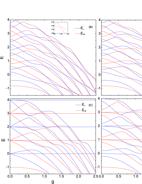
FIG. 3: (Color online) The spectra of two-qubit Rabi model with (a) $\Delta_{1}=0.6$, $\Delta_{2}=0.2$, $\omega=1$, $0\leq g=g_{1}+g_{2}\leq 2.5$, $g_{1}=4g_{2}$.  (b) $\Delta_{1}=0.6$, $\Delta_{2}=0.2$, $\omega=1$, $0\leq g=g_{1}+g_{2}\leq 2.5$, $g_{1}=2g_{2}$. (c)$\Delta_{1}=\Delta_{2}=0.5$, $\omega=1$, $0<g=g_{1}+g_{2}<2.5$, $g_{1}=g_{2}$.  (d)$\Delta_{1}=0.6$, $\Delta_{2}=0.4$, $\omega=1$, $0\leq g\leq 2.5$, $g_{1}=g_{2}$. Blue/Dark grey lines are eigenvalues with odd parity, while red/light grew lines are eigenvalues with even parity.

B Exceptional solutions of the two-qubit quantum Rabi model

From the recurrence relations of $e^{\pm}_{j,n}$ we find two kinds of singular conditions for the eigenvalues at $E=n-(g^{\prime})^{2}$ and $E=n-g^{2}$, which can serve as two kinds of baselines and the second one governs the asymptotics in the deep strong coupling regime of the spectra. Exceptional solutions whose eigenvalues do not correspond to zeros of $G_{\pm}$ occur at the baselines if the parameters satisfy some conditions to lift the singularity of $G_{+}(E)$ or $G_{-}(E)$. In this case, it may happen that the recurrence relations for $e^{\pm}_{j,n}$, (31)–(34), are cutoff at a certain $n$, and the eigenfunctions become polynomials in $z$ if $\alpha=0$. However, not all exceptional states posess this “quasi-exact” form. Unlike the Rabi model, the conditions do not hold for $G_{+}(E)$ and $G_{-}(E)$ at the same time. On the other hand, $G_{+}$ and $G_{-}$ are no longer closely related and level crossings between states of different parity are thus not confined to the baselines.

For identical couplings $g_{1}=g_{2}$ ($g^{\prime}=0$), the coupling term is invariant under permutations of the qubits, which leads to a special kind of exceptional eigenstate. By analyzing the recurrence relations of $e^{\pm}_{j,n}$ for $\alpha=0$, we find polynomial solutions at the baseline $E=N$, where $N$ is a nonnegative integer. These states are very interesting for applications in quantum information theory because they are essentially Fock states, without coherent part as the quasi-exact eigenstates in the Rabi model and the photon number is therefore strictly bounded from above. By considering $\Phi_{1}(z)=\Phi_{3}(-z)$, $\Phi_{2}(z)=\Phi_{4}(-z)$ at $z=0$ and the recurrence relations of $e^{\pm}_{j,n}$ for $\alpha=0$, we find $e^{\pm}_{1,n}=(-1)^{n}e^{\pm}_{3,n}$ and $e^{\pm}_{2,n}=(-1)^{n}e^{\pm}_{4,n}$, and obtain a three term downward recurrence relation for $e^{\pm}_{1,n}$

$$e^{\pm}_{1,n}= g^{-1}[(N-n-1)-\frac{(\Delta_{2}\mp(-1)^{n}\Delta_{1})^{2}}{N-n-1}]e^{\pm}_{1,n+1}$$

$$-(n+2)e^{\pm}_{1,n+2}$$ (8)

with the initial conditions

$$e^{\pm}_{1,N-1}=g^{-1}[\pm(-1)^{N-1}\Delta_{1} -\Delta_{2}]e^{\pm}_{2,N},$$ (9)

$$e^{\pm}_{1,N}=0,$$ (10)

which satisfy $e^{\pm}_{j,n}=0$ for $n>N$. Then we can obtain $e^{\pm}_{1,n}=f^{\pm}(n,N)e^{\pm}_{2,N}$ with non-zero $e^{\pm}_{2,N}$. But $e^{\pm}_{1,-1}$ must vanish if no negative powers of $z$ appear, so $f^{\pm}(-1,N)$ must equal to $0$. As seen from Eq. (8), generally the condition for such states concerns $\Delta_{1}$, $\Delta_{2}$ and $g$ if $\Delta_{1}\neq\Delta_{2}$, e.g., for $N=2$, the condition reads

$$f^{\pm}(-1,2)= [(2-\frac{(\Delta_{1}+\Delta_{2})^{2}}{2})(1-(\Delta_{1}-\Delta_{2})^{2})-g^{2}]$$

$$\times g^{-3}(-\Delta_{1}-\Delta_{2})=0.$$ (11)

This is the condition for an eigenstate with $E=2$ and at most two photons. But it only exists if $\Delta_{1}$ and $\Delta_{2}$ are fine tuned with respect to the coupling $g$. This state is therefore not so easy to prepare in an experiment, because the coupling between the qubits and the radiation field are difficult to control, whereas the qubit level splitting can be tuned very precisely. If states exist where the condition $f^{\pm}(-1,N)=0$ does not depend on $g$, but only on $\Delta_{j}$, they would be very peculiar and interesting for applications.

Indeed, there exist two kinds of such states, with constant eigenenergy for all coupling values. The first kind is the “dark” or “trapping” states rod-lara if $\Delta_{1}=\Delta_{2}$ (see Eq. (9))

$$|\psi\rangle_{ne}=\frac{1}{\sqrt{2}}|n,g,e\rangle-\frac{1}{\sqrt{2}}|n,e,g\rangle.$$ (12)

In this case, the Hamiltonian Eq. (A) possesses the full permutation symmetry between the two spins and the Hilbert space separates naturally into the singlet and the triplet part. The spin singlet decouples from the radiation field, therefore the energy of all singlet states does not depend on the coupling $g$ and the levels cross those of the triplet states which interact with the radiation field. The spectrum for $\Delta_{1}=\Delta_{2}=0.5$, $\omega=1$, $0<g=g_{1}+g_{2}<2.5$, and $g_{1}=g_{2}$ is shown in Fig. 3(c), where $|\psi\rangle_{ne}$ correspond to the horizontal lines at $E=N$. The qubits are in maximally entangled singlet Bell states, which are robust even upon inclusion of dissipation rod-lara . However, this is entirely due to the full decoupling of the singlet states. There is no entanglement between the qubits and the radiation mode.

Now, for the second case, it is quite surprising that a similar state exists even when the full permutation invariance is partially broken: If $g_{1}=g_{2}$ but $\Delta_{1}\neq\Delta_{2}$, only the coupling term is invariant but the qubit energy is not. The function $f^{\pm}(-1,1)$ reads

$$f^{\pm}(-1,1)=g^{-2}(\pm\Delta_{1}-\Delta_{2})[1-(\Delta_{2}\pm\Delta_{1})^{2}],$$ (13)

whose zeros are independent of $g$. So for even parity, if $\Delta_{1}+\Delta_{2}=1$, there exists a state in the exceptional spectrum with $E=1$, independent of $g$, although this state corresponds to strong coupling (and entanglement) between the qubits and the radiation field as its wavefunction does explicitly depend on $g$,

$$|\psi\rangle_{e}=\frac{1}{{\cal N}}\left(\frac{2(\Delta_{1}-\Delta_{2})}{g}|0,e,e\rangle-|1,e,g\rangle+|1,g,e\rangle\right)$$ (14)

with ${\cal N}=\sqrt{4(\Delta_{1}-\Delta_{2})^{2}+2g^{2}}/g$. For odd parity, if $\Delta_{1}-\Delta_{2}=1$ or $\Delta_{2}-\Delta_{1}=1$, there are two corresponding eigenstates

$$|\psi\rangle_{g1}=\frac{1}{{\cal N}}\left(\frac{2(\Delta_{1}+\Delta_{2})}{g}|0,e,g\rangle+|1,g,g\rangle-|1,e,e\rangle\right),$$ (15)

$$|\psi\rangle_{g2}=\frac{1}{{\cal N}}\left(\frac{2(\Delta_{1}+\Delta_{2})}{g}|0,g,e\rangle+|1,g,g\rangle-|1,e,e\rangle\right),$$ (16)

respectively, where ${\cal N}=\sqrt{4(\Delta_{1}+\Delta_{2})^{2}+2g^{2}}/g$. The spectrum of the model for $\Delta_{1}=0.6$, $\Delta_{2}=0.4$, $0<g=g_{1}+g_{2}<2.5$, and $g_{1}=g_{2}$ is shown in Fig. 3(d). The exceptional solution corresponds to the horizontal line of $E=1$, causing level crossings within the same parity subspace, which was discovered numerically by Chilingaryan and Rodríguez-Lara 2bite . These states contain at most one photon, so they are very interesting for single-photon experiments. At the same time, they exist for all coupling values, so they can be prepared without precise knowledge of $g$. The qubit energies can be fine tuned to satisfy the condition $\Delta_{1}+\Delta_{2}=\omega$. One can also obtain these exceptional states in Fock space, as shown in Appendix C.

One may infer from Fig. 3(a) and (b), that there are level crossings in the spectrum between eigenstates with different parity but not for the same parity, so that they can be labeled just by two quantum numbers — energy level and parity, just as in the Rabi model (This, however, has not yet been proven rigorously, see below). However, it has three degrees of freedom and the dimension of the Hilbert space of the discrete degrees of freedom is larger than the number of different parity labels corresponding to the irreducible representations of $\mathbb{Z}_{2}$. This renders the system non-integrable for general values of model parameters br , coinciding with what the narrow avoided crossings in Fig. 3(a) and (b) indicate xu . Level crossings within a given parity subspace are caused by an additional permutation symmetry in Fig. 3(c) and to the symmetry of the qubit-photon couplings in Fig. 3(d). Indeed, due to the possibility that (51) may have a nullspace with dimension $>1$, level crossings in the regular spectrum within a given parity subspace are not ruled out in principle dicke . One notes from Fig. 3(d) the appearance of horizontal baselines, because the singlet is asymptotically decoupled for $g\rightarrow\infty$.

III Solutions of the generalized two-qubit Rabi models

Now we generalize the model by including interactions between the two qubits which are commonly used to generate entanglement gs ; aa , mandatory for applications in quantum computation naga . In our model, entanglement between the qubits is produced naturally by the coupling to the radiation field - nevertheless it is interesting to add a direct interaction term, obtaining more options to control the system. First we will consider the anisotropic XYZ Heisenberg interaction

$$H_{\text{XYZ}}= \omega a^{+}a+g_{1}(a+a^{+})\sigma_{1x}+g_{2}(a+a^{+})\sigma_{2x}$$

$$+\Delta_{1}\sigma_{1z}+\Delta_{2}\sigma_{2z}+\sum_{i=x,y,z}J_{i}\sigma_{1i}\sigma_{2i},$$ (17)

where $J_{x}$, $J_{y}$ and $J_{z}$ are the strength of XYZ Heisenberg interaction in $x$, $y$, $z$ direction respectively. $H_{\text{XYZ}}$ is $\mathbb{Z}_{2}$ invariant under the same transformation as the two-qubit Rabi model. So using the same method as above, we expand the photon field wave functions into the normalized extended coherent state in the parity subspace as $\varphi^{\pm}_{j}=\exp(\alpha^{2}/2)\sum_{n=0}^{\infty}\sqrt{n!}f^{\pm}_{j,n}|n,-\alpha\rangle$ with the recurrence relation of $f^{\pm}_{j,n}$ as Eqs. (84)–(87) in Appendix D. Choosing $\alpha=0$, $g^{\prime}$ and $g$ for this model as above, we can denote $\varphi^{\pm}_{j}(z)$ as $\psi^{\pm}_{j}(z)$, $\phi^{\pm}_{j}(z)$ and $\Phi^{\pm}_{j}(z)$ respectively. Similarly, there are eight equations

$$\phi^{\pm}_{j}(z_{0})=\psi^{\pm}_{j}(z_{0}),~{}\phi^{\pm}_{j}(z^{\prime}_{0})=\Phi^{\pm}_{j}(z^{\prime}_{0})$$ (18)

for eight free initial conditions $\{f^{\pm,\alpha=0}_{1,0}$, $f^{\pm,\alpha=0}_{2,0}$, $f^{\pm,\alpha=g^{\prime}}_{1,0}$, $f^{\pm,\alpha=g^{\prime}}_{2,0}$, $f^{\pm,\alpha=g^{\prime}}_{3,0}$, $f^{\pm,\alpha=g}_{1,0}$, $f^{\pm,\alpha=g}_{2,0}$, $f^{\pm,\alpha=g}_{4,0}\}$, similar to Eq. (51). The determinant which is the function of eigenvalue $E$ must be zero if non-trivial solutions to the equations exist. So the eigenvalues and eigenstates are obtained. From Eqs. (86) and (87) we find there are two kinds of baselines located at $E=n-g^{2}+J_{x}$ and $E=n-(g^{\prime})^{2}-J_{x}$. The first kind of baselines governs the asymptotics for strong coupling. For XXX Heisenberg interaction and dipole interaction, we just need to set $J_{x}=J_{y}=J_{z}$ and $J_{x}=\epsilon$, $J_{y}=J_{z}=0$ respectively. The lowest part of the spectra for four sets of parameters are shown in Fig. 4. The narrow avoid crossing in Fig. 4(a) shows the non-integrability of this model xu , just like the two-qubit Rabi model.

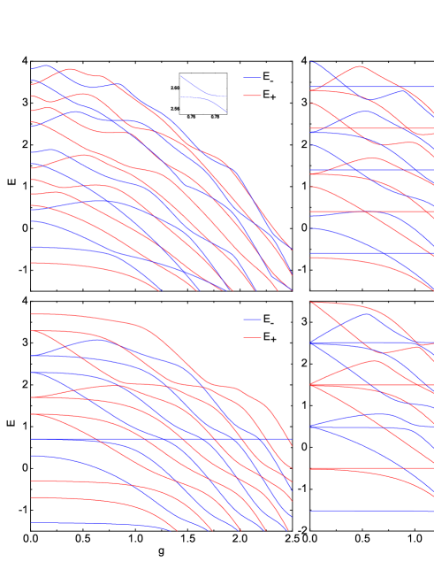
FIG 4: (Color online) The spectra of the generalized two-qubit Rabi models with (a) $\Delta_{1}=0.6$, $\Delta_{2}=0.2$, $\omega=1$, $0<g=g_{1}+g_{2}<2.5$, $g_{1}=4g_{2}$, $J_{x}=0.2,~{}J_{y}=0.0,~{}J_{z}=0.0$. (b) $\Delta_{1}=0.5$, $\Delta_{2}=0.5$, $\omega=1$, $0<g=g_{1}+g_{2}<2.5$, $g_{1}=g_{2}$, $J_{x}=0.1,~{}J_{y}=0.2,~{}J_{z}=0.3$. (c) $\Delta_{1}=0.1$, $\Delta_{2}=0.7$, $\omega=1$, $0<g=g_{1}+g_{2}<2.5$, $g_{1}=g_{2}$, $J_{x}=0.7,~{}J_{y}=0.1,~{}J_{z}=0.3$. (d) $\Delta_{1}=0.6$, $\Delta_{2}=0.4$, $\omega=1$, $0<g=g_{1}+g_{2}<2.5$, $g_{1}=g_{2}$, $J_{x}=0.5,~{}J_{y}=0.5,~{}J_{z}=0.5$. Blue/Dark grey lines are eigenvalues with odd parity, while red/light grew lines are eigenvalues with even parity.

For the special case: $g^{\prime}=0$, i.e. $g_{1}=g_{2}$, we only need to choose $\alpha=0$ and $g$, and there are four equations

$$\Phi^{\pm}_{j}(z_{0})=\psi^{\pm}_{j}(z_{0})$$ (19)

for four free initial conditions $\{f^{\pm,\alpha=0}_{1,0}$, $f^{\pm,\alpha=g}_{1,0}$, $f^{\pm,\alpha=g}_{2,0}$, $f^{\pm,\alpha=g}_{4,0}\}$. Similar to the two-qubit Rabi model, we find $f^{\pm}_{1,n}=(-1)^{n}f^{\pm}_{3,n}$ and $f^{\pm}_{2,n}=(-1)^{n}f^{\pm}_{4,n}$. There are three kinds of base lines located at $E=n-g^{2}+J_{x}$ and $E=n-J_{x}\pm J_{y}\pm J_{z}$. As usual, exceptional solutions are located on the baselines if parameters satisfy an additional constraint.

As in the non-interacting case, there exist exceptional solutions independent of $g$ with constant eigenenergy. The condition just concerns the qubits energy and qubit-qubit interaction strength. As discussed above, by analyzing the recurrence relations of $f^{\pm}_{j,n}$ for $\Phi^{\pm}_{j}(z)$ ($\alpha$, $g^{\prime}=0$), we find exceptional solutions as polynomials in $z$ for $E=N-J_{x}\pm(-1)^{N}J_{y}\pm(-1)^{N}J_{z}$, where $N$ is a nonnegative integer. For these states, the recurrence relations of $f^{\pm}_{j,n}$ for $\alpha=0$ satisfy $f^{\pm}_{j,n}=0$ for $n>N$, and we find the three term downward recurrences for $f^{\pm}_{1,n}$

$$f^{\pm}_{1,n}= g^{-1}[\frac{-(\Delta_{2}\pm(-1)^{n+1}\Delta_{1})^{2}}{N-n-1\pm((-1)^{N}+(-1)^{n})(J_{y}+J_{z})}$$

$$\pm((-1)^{N}-(-1)^{n})J_{y}\pm((-1)^{N}+(-1)^{n})J_{z}$$

$$+N-n-1-2J_{x}]f^{\pm}_{1,n+1}-(n+2)f^{\pm}_{1,n+2}$$ (20)

with the initial condition

$$f^{\pm}_{1,N-1}=g^{-1}[\pm(-1)^{N-1}\Delta_{1} -\Delta_{2}]f^{\pm}_{2,N},$$ (21)

$$f^{\pm}_{1,N}=0,$$ (22)

so that we can obtain $f^{\pm}_{1,n}=m^{\pm}(n,N)f^{\pm}_{2,N}$ with non-zero $f^{\pm}_{2,N}$. But $f^{\pm}_{1,-1}$ must vanish if no negative powers of $z$ appear, so $m^{\pm}(-1,N)=0$. As seen from Eq. (20), this will give some constraint on $g$ in general, but for $\Delta_{1}=\Delta_{2}$ (see Eq. (21)), the singlet Bell state $|\psi\rangle_{n}$ is still the eigenstate with eigenenergy $E=n-J_{x}-J_{y}-J_{z}$, shown in Fig. 4(b). They are robust and survive the inclusion of XYZ Heisenberg interaction because $\sum_{i=x,y,z}J_{i}\sigma_{1i}\sigma_{2i}|\psi\rangle_{n}=-(J_{x}+J_{y}+J_{z})|\psi\rangle_{n}$. However, they are not entangled with the radiation field. For $N=1$, we obtain

$$m^{\pm}(-1,1)=g^{-2}(\pm\Delta_{1}-\Delta_{2})[(J_{x}\pm J_{y}\pm 2J_{z}-1)^{2}$$

$$-(J_{x}\mp J_{y})^{2}-(\Delta_{2}\pm\Delta_{1})^{2}]/(1-2J_{y}-2J_{z})=0,$$ (23)

which is independent of $g$. So under this condition, there exists an entangled eigenstate with even parity,

$$|\psi\rangle_{e1}= \frac{1}{\mathcal{N}}[(1-2J_{y}-2J_{z}-\Delta_{1}-\Delta_{2})|0,g,g\rangle$$

$$+(1-2J_{y}-2J_{z}+\Delta_{1}+\Delta_{2})|0,e,e\rangle$$

$$+\frac{(1-2J_{y}-2J_{z})g}{\Delta_{1}-\Delta_{2}}(|1,g,e\rangle-|1,e,g\rangle)],$$ (24)

with eigenenergy $E=1-J_{x}-J_{y}-J_{z}$ in the whole coupling regime, where $\frac{1}{\mathcal{N}}$ is a normalizing constant. For odd parity, we just need to change the sign of $J_{y}$, $J_{z}$, $\Delta_{1}$, and the spin direction of the first qubit in $|\psi\rangle_{e1}$, corresponding to the horizontal line in Fig. 4(c). If $J_{x}=J_{y}=J_{z}=0$, $|\psi\rangle_{e1}$ reduces to $|\psi\rangle_{e}$. Even more interestingly, we find in the special case $J_{x}\pm J_{y}\pm 2J_{z}=2$,

$$m^{\pm}(-1,3)=0,$$ (25)

for the same parameters which yield $m^{\pm}(-1,1)=0$. This corresponds to a second exceptional state with eigenenergy $E=3-J_{x}\mp J_{y}\mp J_{z}$ in the spectrum for arbitrary coupling. This eigenstate reads for even parity,

$$|\psi\rangle_{e3}=\frac{1}{\mathcal{M}}[(3-2J_{y}-2J_{z}-\Delta_{1}-\Delta_{2})|0,g,g\rangle$$

$$+(3-2J_{y}-2J_{z}+\Delta_{1}+\Delta_{2})|0,e,e\rangle$$

$$+\frac{(2J_{y}+2J_{z}-3)(1-2J_{y}-2J_{z}-\Delta_{2}-\Delta_{1})}{\sqrt{2}(1-2J_{y}-2J_{z})}|2,g,g\rangle$$

$$+\frac{(2J_{y}+2J_{z}-3)(1-2J_{y}-2J_{z}+\Delta_{2}+\Delta_{1})}{\sqrt{2}(1-2J_{y}-2J_{z})}|2,e,e\rangle$$

$$+\frac{\sqrt{6}(2J_{y}+2J_{z}-3)g}{2(\Delta_{1}-\Delta_{2})}(|3,g,e\rangle-|3,e,g\rangle)],$$ (26)

where $\frac{1}{\mathcal{M}}$ is the normalizing constant. In this case the spectrum contains two horizontal lines intersecting all other levels, as shown in Fig. 4(d).

IV Conclusion

We have studied the asymmetric two-qubit quantum Rabi model and include (anisotropic) Heisenberg interactions between the qubits. The spectra and eigenstates are obtained analytically using Bargmann-space techniques. An equivalent alternative to this solution of the two-qubit Rabi model is the method based on the normalized extended coherent states qing $|n,-\alpha\rangle$, while continued-fraction techniques schweb ; swa are not applicable. All models possess a parity symmetry, but this is not sufficient for integrability because the discrete state space is four-dimensional, whereas there are only two different parity labels. We observe no level crossings in the regular spectrum within the same parity chain (although they are not ruled out in principle dicke ), and the narrow avoided crossings indicate thus the non-integrability of the model, consistent with the criterion proposed in br . For special values of the qubit transition frequencies, there exist exceptional solutions which cause level crossings within the subspaces with fixed parity, reminiscent of the quasi-exact solutions present in the Rabi model, but closely related to the singlet states in the model with unbroken permutation invariance. These simply structured eigenstates may be easily prepared in current experimental set-ups because the condition for their existence involves only the qubit energy splittings $\Delta_{j}$ and not the coupling $g$ to the radiation field. This makes them especially well suited for applications in quantum storage and transfer. The algebraic structure behind the possibility of this novel type of exceptional eigenstate needs further clarification. We may conjecture that the new class of states exists only for an even number of qubits, where the permutationally invariant model possesses a singlet sector.

Appendix A Solution of the model without qubit interaction

First, we give some details about obtaining the recurrence relations of $e^{\pm}_{j,n}$. In the Bargmann space, the eigenvalue equations are reduced to four coupled differential equations as

$$(z+g)\frac{{\rm d}}{{\rm d}z}\varphi^{\pm}_{1} =(E-gz)\varphi^{\pm}_{1}\mp\Delta_{1}\varphi^{\pm}_{4}-\Delta_{2}\varphi^{\pm}_{2},$$ (27)

$$(z+g^{\prime})\frac{{\rm d}}{{\rm d}z}\varphi^{\pm}_{2} =(E-g^{\prime}z)\varphi^{\pm}_{2}\mp\Delta_{1}\varphi^{\pm}_{3}-\Delta_{2}\varphi^{\pm}_{1},$$ (28)

$$(z-g)\frac{{\rm d}}{{\rm d}z}\varphi^{\pm}_{3} =(E+gz)\varphi^{\pm}_{3}\mp\Delta_{1}\varphi^{\pm}_{2}-\Delta_{2}\varphi^{\pm}_{4},$$ (29)

$$(z-g^{\prime})\frac{{\rm d}}{{\rm d}z}\varphi^{\pm}_{4} =(E+g^{\prime}z)\varphi^{\pm}_{4}\mp\Delta_{1}\varphi^{\pm}_{1}-\Delta_{2}\varphi^{\pm}_{3},$$ (30)

where $g=g_{1}+g_{2}$, $g^{\prime}=g_{1}-g_{2}$. Expanding $\varphi^{\pm}_{j}$ ($j=1$, $\ldots$, $4$) as $\varphi^{\pm}_{j}=e^{\alpha^{2}/2}\sum_{n=0}^{\infty}\sqrt{n!}e^{\pm}_{j,n}|n,-\alpha\rangle$, and substituting it into Eqs. (27)–(30), we find the recurrence relations for $e^{\pm}_{j,n}$

$$(\alpha+g)(n+1)e^{\pm}_{1,n+1} =(E-n-2\alpha g-\alpha^{2})e^{\pm}_{1,n}-(\alpha+g)e^{\pm}_{1,n-1}\mp\Delta_{1}e^{\pm}_{4,n}-\Delta_{2}e^{\pm}_{2,n},$$ (31)

$$(\alpha+g^{\prime})(n+1)e^{\pm}_{2,n+1} =(E-n-2\alpha g^{\prime}-\alpha^{2})e^{\pm}_{2,n}-(\alpha+g^{\prime})e^{\pm}_{2,n-1}\mp\Delta_{1}e^{\pm}_{3,n}-\Delta_{2}e^{\pm}_{1,n},$$ (32)

$$(\alpha-g)(n+1)e^{\pm}_{3,n+1} =(E-n+2\alpha g-\alpha^{2})e^{\pm}_{3,n}-(\alpha-g)e^{\pm}_{3,n-1}\mp\Delta_{1}e^{\pm}_{2,n}-\Delta_{2}e^{\pm}_{4,n},$$ (33)

$$(\alpha-g^{\prime})(n+1)e^{\pm}_{4,n+1} =(E-n+2\alpha g^{\prime}-\alpha^{2})e^{\pm}_{4,n}-(\alpha-g^{\prime})e^{\pm}_{4,n-1}\mp\Delta_{1}e^{\pm}_{1,n}-\Delta_{2}e^{\pm}_{3,n},$$ (34)

Then we show the details of obtaining the eigenvalue $E$ with Eq. (4). To have a more convenient form for practical calculation, we denote $\phi^{\pm}_{j}(z)=\sum_{k}e^{\pm}_{k,0}\phi_{j}^{k\pm}(z)$, $k=1$, $2$, $3$, $\psi^{\pm}_{j}(z)=\sum_{l}e^{\prime\pm}_{l,0}\psi_{j}^{l\pm}(z)$, $l=1$, $2$, $4$, and $\Phi_{j}(z)=\sum_{m}e^{\prime\prime\pm}_{m,0}\Phi_{j}^{m\pm}(z)$, $m=1$, $2$, as in dicke , where for example, $\phi_{j}^{1\pm}(z)$ is obtained by setting $e^{\pm}_{1,0}=1$ and $e^{\pm}_{2,0}$, $e^{\pm}_{3,0}=0$ in linear equations (31)–(34). Eqs. (4) take the form of the following linear system

$$\left(\begin{array}[]{cccccccc}\psi_{1}^{1\pm}(z_{0})&\psi_{1}^{2\pm}(z_{0})&\psi_{1}^{3\pm}(z_{0})&-\phi_{1}^{1\pm}(z_{0})&-\phi_{1}^{2\pm}(z_{0})&-\phi_{1}^{3\pm}(z_{0})&0&0\\ \psi_{2}^{1\pm}(z_{0})&\psi_{2}^{2\pm}(z_{0})&\psi_{2}^{3\pm}(z_{0})&-\phi_{2}^{1\pm}(z_{0})&-\phi_{2}^{2\pm}(z_{0})&-\phi_{2}^{3\pm}(z_{0})&0&0\\ \psi_{3}^{1\pm}(z_{0})&\psi_{3}^{2\pm}(z_{0})&\psi_{3}^{3\pm}(z_{0})&-\phi_{3}^{1\pm}(z_{0})&-\phi_{3}^{2\pm}(z_{0})&-\phi_{3}^{3\pm}(z_{0})&0&0\\ \psi_{4}^{1\pm}(z_{0})&\psi_{4}^{2\pm}(z_{0})&\psi_{4}^{3\pm}(z_{0})&-\phi_{4}^{1\pm}(z_{0})&-\phi_{4}^{2\pm}(z_{0})&-\phi_{4}^{3\pm}(z_{0})&0&0\\ 0&0&0&\phi_{1}^{1\pm}(z^{\prime}_{0})&\phi_{1}^{2\pm}(z^{\prime}_{0})&\phi_{1}^{3\pm}(z^{\prime}_{0})&-\Phi_{1}^{1\pm}(z^{\prime}_{0})&-\Phi_{1}^{2\pm}(z^{\prime}_{0})\\ 0&0&0&\phi_{2}^{1\pm}(z^{\prime}_{0})&\phi_{2}^{2\pm}(z^{\prime}_{0})&\phi_{2}^{3\pm}(z^{\prime}_{0})&-\Phi_{2}^{1\pm}(z^{\prime}_{0})&-\Phi_{2}^{2\pm}(z^{\prime}_{0})\\ 0&0&0&\phi_{3}^{1\pm}(z^{\prime}_{0})&\phi_{3}^{2\pm}(z^{\prime}_{0})&\phi_{3}^{3\pm}(z^{\prime}_{0})&-\Phi_{3}^{1\pm}(z^{\prime}_{0})&-\Phi_{3}^{2\pm}(z^{\prime}_{0})\\ 0&0&0&\phi_{4}^{1\pm}(z^{\prime}_{0})&\phi_{4}^{2\pm}(z^{\prime}_{0})&\phi_{4}^{3\pm}(z^{\prime}_{0})&-\Phi_{4}^{1\pm}(z^{\prime}_{0})&-\Phi_{4}^{2\pm}(z^{\prime}_{0})\end{array}\right)\left(\begin{array}[]{c}e^{\pm}_{1,0}\\ e^{\pm}_{2,0}\\ e^{\pm}_{4,0}\\ e^{\prime\pm}_{1,0}\\ e^{\prime\pm}_{2,0}\\ e^{\prime\pm}_{3,0}\\ e^{\prime\prime\pm}_{1,0}\\ e^{\prime\prime\pm}_{2,0}\end{array}\right)=0.$$ (51)

For (51) to have a non-trivial solution, the determinant of the above $8*8$ matrix must vanish, which determines the eigenvalue $E$.

For the convergent powerseries, one chooses $z_{0}^{\prime}\in D_{1}$, however, it is remarkable that if we choose $z_{0}^{\prime}\notin D_{1}$, we can still obtain correct eigenvalues $E_{n}$. If we choose large enough truncating order $n_{max}$, the zero of $G_{\pm}$ will converge to the correct value even though the power series is not convergent, because the wave functions are holomorphic in $\mathbb{C}$ exactly at $E_{n}$, entailing a convergent power series expansion at $z^{\prime}_{0}$ outside of $D_{1}$ braak . However, because the power series are not convergent, one will encounter very large values for the $\phi_{j}(z_{0}^{\prime})$, rendering it not as convenient as the convergent one for small eigenenergies.

Appendix B Solution obtained with extended coherent states method

An alternative to the solution of the two-qubit Rabi model presented here is the method based on normalized extended coherent states qing $|n,-\alpha\rangle$, which is the eigenstate of $(a^{\dagger}-\alpha)(a-\alpha)$. Defining $A^{\dagger}=a^{\dagger}-\alpha$, we can rewrite the Hamiltonian (2) in the positive parity space as

$$H_{+}= A^{\dagger}A+\alpha^{2}+\alpha(A+A^{\dagger})+\Delta_{2}\sigma_{2x}+\Delta_{1}\sigma_{2x}R+(A+A^{\dagger}+2\alpha)(g_{1}+g_{2}\sigma_{2z}).$$ (52)

We expand it in the diagonal presentation of $\sigma_{2z}$. Then using the time independent Schrödinger equation, making the transformation $R=\exp(i\pi a^{\dagger}a)$ on it, and denoting $\varphi_{3}=R\varphi_{1}$, $\varphi_{4}=R\varphi_{2}$, we obtain four equations

$$[A^{\dagger}A+\alpha^{2}+2\alpha g+(g+\alpha)(A+A^{\dagger})-E]\varphi_{1}+\Delta_{2}\varphi_{2}+\Delta_{1}\varphi_{4}=0,$$ (53)

$$[A^{\dagger}A+\alpha^{2}+2\alpha g^{\prime}+(g^{\prime}+\alpha)(A+A^{\dagger})-E]\varphi_{2}+\Delta_{2}\varphi_{1}+\Delta_{1}\varphi_{3}=0,$$ (54)

$$[A^{\dagger}A+\alpha^{2}-2\alpha g-(g-\alpha)(A+A^{\dagger})-E]\varphi_{3}+\Delta_{2}\varphi_{4}+\Delta_{1}\varphi_{2}=0,$$ (55)

$$[A^{\dagger}A+\alpha^{2}-2\alpha g^{\prime}-(g^{\prime}-\alpha)(A+A^{\dagger})-E]\varphi_{2}+\Delta_{2}\varphi_{3}+\Delta_{1}\varphi_{1}=0,$$ (56)

where $g=g_{1}+g_{2}$, $g^{\prime}=g_{1}-g_{2}$. Then we expand $\varphi_{j}$, $j=1,2,3,4,$ in terms of the orthogonal extended coherent state as $\varphi_{j}=e^{\alpha^{2}/2}\sum_{m=0}^{\infty}\sqrt{m!}e_{j,m}|m,-\alpha\rangle$, and left multiply $|n,-\alpha\rangle$, we obtain the recursion relations for $e_{j,n}$ which are the same as Eqs. (31)–(34).

In order to limit the number of free initial conditions, we choose $\alpha=g,g^{\prime},0$, then we obtain three expansions of the wavefunction. They can be different only by a constant, which can be chosen as 1, because the linearity of Eqs. (53)–(56). For $\alpha=g^{\prime}$, we have $\phi_{j}=e^{(g^{\prime})^{2}/2}\sum_{n=0}^{\infty}\sqrt{n!}a_{j,n}|n,-g^{\prime}\rangle$. For $\alpha=g$, we have $\psi_{j}=e^{g^{2}/2}\sum_{n=0}^{\infty}\sqrt{n!}\sum_{n=0}^{\infty}b_{j,n}|n,-g\rangle$ and for $\alpha=0$, we have $\Psi_{j}=\sum_{n=0}^{\infty}\sqrt{n!}\sum_{n=0}^{\infty}c_{j,n}|n\rangle$. If we left multiply the basic vector of the Bargmann space $\langle 0|e^{\beta a}$, we have

$$\langle 0|e^{\beta a}\varphi_{j}=\sum_{n=0}^{\infty}e_{j,n}\exp(\alpha\beta)(\beta-\alpha)^{n}.$$ (57)

As discussed in the Bargmann space, we have $8$ equations

$$\langle 0|e^{\beta_{1}a}\phi_{j}=\langle 0|e^{\beta_{1}a}\psi_{j},~{}\langle 0|e^{\beta_{2}a}\phi_{j}=\langle 0|e^{\beta_{2}a}\Phi_{j}$$ (58)

for $8$ initial conditions $\{b_{1,0},b_{2,0},b_{4,0},a_{1,0},a_{2,0},a_{3,0},c_{1,0},c_{2,0}\}$. To have a convergent expansion series, we choose $(\beta-\alpha)<R_{\alpha}$, where $R_{\alpha}$ is the convergent radius of $e_{j,n}$. So according to the analysis in the Bargmann space, we can choose $\beta_{1}=z_{0}$ and $\beta_{2}=z_{0}^{\prime}$ to obtain the some eigenvalue and eigenstate as in the Bargmann space. We can also choose $\alpha=-g,-g^{\prime},0$ and the results will be the same.

Appendix C $E=N$ exceptional solution in Fock space

In this appendix, we try to obtain the $g$-independent exceptional solution in Fock space. If for example, $M$ and $N$ are even, the Hamiltonian in a closed odd parity basis of $\{|M,e,g\rangle,|M,g,e\rangle,|M+1,g,g\rangle,|M+1,e,e\rangle,\cdots,|N-1,g,g\rangle,|N-1,e,e\rangle,|N,e,g\rangle,|N,g,e\rangle$ reads

$$\left(\begin{array}[]{ccccccc}0&0&\sqrt{M-1}g_{1}&\sqrt{M-1}g_{2}&0&0&\dots\\ 0&0&\sqrt{M-1}g_{2}&\sqrt{M-1}g_{1}&0&0&\dots\\ \sqrt{M-1}g_{1}&\sqrt{M-1}g_{2}&M+\Delta_{1}-\Delta_{2}&0&\sqrt{M}g_{1}&\sqrt{M}g_{2}&\dots\\ \sqrt{M-1}g_{2}&\sqrt{M-1}g_{1}&0&M+\Delta_{2}-\Delta_{1}&\sqrt{M}g_{2}&\sqrt{M}g_{1}&\dots\\ {7}\end{array}\right)$$ (64)

$$\left(\begin{array}[]{ccccccc}{7}\\ \dots&\sqrt{N}g_{1}&\sqrt{N}g_{2}&N+\Delta_{1}-\Delta_{2}&0&\sqrt{N+1}g_{1}&\sqrt{N+1}g_{2}\\ \dots&\sqrt{N}g_{2}&\sqrt{N}g_{1}&0&N+\Delta_{2}-\Delta_{1}&\sqrt{N+1}g_{2}&\sqrt{N+1}g_{1}\\ \dots&0&0&\sqrt{N+1}g_{1}&\sqrt{N+1}g_{2}&0&0\\ \dots&0&0&\sqrt{N+1}g_{2}&\sqrt{N+1}g_{1}&0&0\end{array}\right).$$ (70)

To have a closed subspace, the coefficients of $|N+1,g,g\rangle$ and $|N+1,e,e\rangle$ must be zero, so we have

$$\sqrt{N+1}\large{g}_{\scriptstyle 1}\large{c}_{1,N}+\sqrt{N+1}g_{2}c_{2,N}=0,$$ (71)

$$\sqrt{N+1}g_{2}c_{1,N}+\sqrt{N+1}g_{1}c_{2,N}=0,$$ (72)

where $c_{1,N},c_{2,N}$ are the coefficients of $|N,e,g\rangle,|N,g,e\rangle$ respectively. From Eqs. (71) and (72) and $g_{1}$, $g_{2}>0$ we obtain $g_{1}=g_{2}$ and $c_{1,N}=-c_{2,N}$. With the time-independent Schrödinger equation, we obtain

$$\sqrt{N}g_{1}c_{1,N-1}+\sqrt{N}g_{2}c_{2,N-1}+(N+\Delta_{1}-\Delta_{2})c_{1,N}=Ec_{1,N},$$ (73)

$$\sqrt{N}g_{2}c_{1,N-1}+\sqrt{N}g_{1}c_{2,N-1}+(N+\Delta_{2}-\Delta_{1})c_{2,N}=Ec_{2,N},$$ (74)

from which we can obtain

$$E =N$$ (75)

$$(\Delta_{2}-\Delta_{1})c_{1,N} =(\sqrt{N}g_{1}c_{1,N-1}+\sqrt{N}g_{2}c_{2,N-1}).$$ (76)

If $\Delta_{1}=\Delta_{2}$ and $c_{1,N-1}=c_{2,N-1}=0$, the eigenstate becomes $|\psi\rangle_{N}=\frac{1}{\sqrt{2}}(|N,g,e\rangle-|N,e,g\rangle)$, the well known “dark state” or “trapping state” rod-lara . Else, in order to have a closed subspace, the coefficients of $|M-1,g,g\rangle$ and $|M-1,e,e\rangle$ must be $0$, so we obtain $E=M$ using the time-independent Schrödinger equation as above, which contradict the condition $E=N$. So, we can only choose $M=0$, where $|M-1,e,e\rangle$ vanish automatically. There is a special case: $M=0$ and $N=1$, then it is required $\Delta_{1}-\Delta_{2}=1=N$ or $\Delta_{2}-\Delta_{1}=1=N$, and the corresponding eigenstates are $|\psi\rangle_{g1}$ (see Eq. (15)) and $|\psi\rangle_{g2}$ (see Eq. (16)) respectively. For even parity case, it is required that $\Delta_{1}+\Delta_{2}=1$ or $-\Delta_{1}-\Delta_{2}=1$. The second condition can not be satisfied, so we find only one exceptional eigenstate $|\psi\rangle_{e}$ (see Eq. (14)).

Appendix D The recurrence relations of $f^{\pm}_{j,n}$

First we make unitary transformations $S=\frac{1}{\sqrt{2}}(\sigma_{x}+\sigma_{z})$ to $H_{\text{XYZ}}$ to interchange $\sigma_{x}$ and $\sigma_{z}$ and obtain $H^{\prime}_{\text{XYZ}}$. Applying the same Fulton-Gouterman transformation U pj ; fg as above, we obtain

$$U^{\dagger}H^{\prime}_{\text{XYZ}}U=\left(\begin{array}[]{cc}H_{\text{XYZ}+}&0\\ 0&H_{\text{XYZ}-}\\ \end{array}\right),$$ (79)

where $H_{\text{XYZ}\pm}=z\partial_{z}+g_{1}(z+\partial_{z})+g_{2}(z+\partial_{z})\sigma_{2z}+\Delta_{2}\sigma_{2x}+J_{x}\sigma_{2z}\pm\Delta_{1}R\sigma_{2x}\mp J_{y}R\sigma_{2z}\pm J_{z}R$ for two invariant subspaces with eigenvalues of $R^{\prime}$ being $\pm 1$ respectively. We expand it in the diagonal representation of $\sigma_{2z}$, denoting $\varphi^{\pm}_{3,4}(z)=\varphi^{\pm}_{1,2}(-z)$, making the transformation $z\rightarrow-z$ and obtain the time-independent Schrödinger equations

$$(z+g)\frac{z}{dz}\varphi^{\pm}_{1} =(E-J_{x}-gz)\varphi^{\pm}_{1}\mp(J_{z}-J_{y})\varphi^{\pm}_{3}-\Delta_{2}\varphi^{\pm}_{2}\mp\Delta_{1}\varphi^{\pm}_{4},$$ (80)

$$(z+g^{\prime})\frac{z}{dz}\varphi^{\pm}_{2} =(E+J_{x}-g^{\prime}z)\varphi^{\pm}_{2}\mp(J_{z}+J_{y})\varphi_{4}-\Delta_{2}\varphi^{\pm}_{1}\mp\Delta_{1}\varphi^{\pm}_{3},$$ (81)

$$(z-g)\frac{z}{dz}\varphi^{\pm}_{3} =(E-J_{x}+gz)\varphi^{\pm}_{3}\mp(J_{z}-J_{y})\varphi^{\pm}_{1}-\Delta_{2}\varphi^{\pm}_{4}\mp\Delta_{1}\varphi^{\pm}_{2},$$ (82)

$$(z-g^{\prime})\frac{z}{dz}\varphi^{\pm}_{4} =(E+J_{x}+g^{\prime}z)\varphi^{\pm}_{4}\mp(J_{z}+J_{y})\varphi^{\pm}_{2}-\Delta_{2}\varphi^{\pm}_{3}\mp\Delta_{1}\varphi^{\pm}_{1}.$$ (83)

We expand the photon field wave functions into the normalized extended coherent state in the parity subspace as $\varphi^{\pm}_{j}=\exp(\alpha^{2}/2)\sum_{n=0}^{\infty}\sqrt{n!}f^{\pm}_{j,n}|n,-\alpha\rangle$ and substitute them into Eqs. (80)–(83) to obtain the recurrence relations for $f^{\pm}_{j,n}$

$$(n+1)(g+\alpha)f^{\pm}_{1,n+1}= (E-n-\alpha^{2}-2\alpha g-J_{x})f^{\pm}_{1,n}-(\alpha+g)f^{\pm}_{1,n-1}-\Delta_{2}f^{\pm}_{2,n}\mp\Delta_{1}f^{\pm}_{4,n}\mp(J_{z}-J_{y})f^{\pm}_{3,n},$$ (84)

$$(n+1)(\alpha+g^{\prime})f^{\pm}_{2,n+1}= (E-n-\alpha^{2}-2\alpha g^{\prime}+J_{x})f^{\pm}_{2,n}-(\alpha+g^{\prime})f^{\pm}_{2,n-1}-\Delta_{2}f^{\pm}_{1,n}\mp\Delta_{1}f^{\pm}_{3,n}\mp(J_{y}+J_{z})f^{\pm}_{4,n},$$ (85)

$$(n+1)(\alpha-g)f^{\pm}_{3,n+1}= (E-n-\alpha^{2}+2\alpha g-J_{x})f^{\pm}_{3,n}-(\alpha-g)f^{\pm}_{3,n-1}-\Delta_{2}f^{\pm}_{4,n}\mp\Delta_{1}f^{\pm}_{2,n}\mp(J_{z}-J_{y})f^{\pm}_{1,n},$$ (86)

$$(n+1)(\alpha-g^{\prime})f^{\pm}_{4,n+1}= (E-n-\alpha^{2}+2\alpha g^{\prime}+J_{x})f^{\pm}_{4,n}-(\alpha-g^{\prime})f^{\pm}_{4,n-1}-\Delta_{2}f^{\pm}_{3,n}\mp\Delta_{1}f^{\pm}_{1,n}\mp(J_{y}+J_{z})f^{\pm}_{2,n}.$$ (87)

which are then analyzed in a similar way as the $e^{\pm}_{j,n}$ in Appendix A.

References

- (1) E. T. Jaynes, and F. W. Cummings, Proc. IEEE 51, 89 (1963).
- (2) X. Y. Guo and S.-C. Lü, Phys. Rev. A 80, 043826 (2009); X. Y. Guo and Z. Z. Ren, Phys. Rev. A 83, 013809 (2011); X. Y. Guo, Z. Z. Ren, and Z. M. Chi, Phys. Rev. A 85, 023608 (2012).
- (3) T. Werlang, A. V. Dodonov, E. I. Duzzioni, and C. J. Villas-Bôas, Phys. Rev. A 78, 053805 (2008).
- (4) I. Lizuain, J. Casanova, J. J. García-Ripoll, J. G. Muga, and E. Solano, Phys. Rev. A 81, 062131 (2010); G. Romero, I. Lizuain, V. S. Shumeiko, E. Solano, and F. S. Bergeret, Phys. Rev. B 85, 180506 (2012).
- (5) T. Grujic, S. R. Clark, D. Jaksch, and D. G. Angelakis, New J. Phys. 14, 103025 (2012).
- (6) S. B. Zheng, Phys. Rev. A 86, 012326(2012).
- (7) A. C. Doherty, A. S. Parkins, S. M. Tan, and D. F. Walls, J. Opt. B: Quantum Semiclass. Opt. 1, 475 (1999).
- (8) I-H. Chen, Y. Y. Lin, Y.-C. Lai, E. S. Sedov, A. P. Alodjants, S. M. Arakelian, and R.-K. Lee, Phys. Rev. A 86, 023829 (2012).
- (9) A. Janutka, J. Phys. A: Math. Gen. 39, 577 (2006).
- (10) S. Schweber, Ann. Phys. (N.Y.) 41, 205 (1967).
- (11) S. Swain, J. Phys. A 6, 192, 1919 (1973).
- (12) I. Travěnec, and L. Šamaj, Phys. Lett. A 375, 4104 (2011).
- (13) V. V. Albert, G. D. Scholes, and P. Brumer, Phys. Rev. A 84, 042110 (2011).
- (14) D. Braak, Phys. Rev. Lett. 107, 100401 (2011).
- (15) V. Bargmann, Comm. Pure Appl. Math. 14, 187 (1961).
- (16) J. Casanova, G. Romero, I. Lizuain, J. J. García-Ripoll, and E. Solano, Phys. Rev. Lett. 105, 263603 (2010).
- (17) D. Ballester, G. Romero, J. J. García-Ripoll, F. Deppe, and E. Solano, Phys. Rev. X 2, 021007 (2012).
- (18) F. A. Wolf, M. Kollar, and D. Braak, Phys. Rev. A 85, 053817 (2012).
- (19) F. A. Wolf, F. Vallone, G. Romero, M. Kollar, E. Solano, and D. Braak, Phys. Rev. A 87, 023835 (2013)
- (20) L. X. Yu, S. Q. Zhu, Q. F. Liang, G. Chen, and S. T. Jia, Phys. Rev. A 86, 015803 (2012).
- (21) Q.-H. Chen, C. Wang, S. He, T. Liu, and K.-L. Wang, Phys. Rev. A 86, 023822 (2012).
- (22) D. Braak, J. Phys. A: Math. Theor. 46, 175301 (2013).
- (23) I. Travěnec, Phys. Rev. A 85, 043805 (2012).
- (24) J. Peng, Z. Z. Ren, G. J. Guo, and G. X. Ju, J. Phys. A: Math. Theor. 45, 365302 (2012).
- (25) S. A. Chilingaryan and B. M. Rodríguez-Lara, J. Phys. A: Math. Theor. 46, 335301 (2013).
- (26) J. Peng, Z. Z. Ren, G. J. Guo, G. X. Ju and X. Y. Guo, Eur. Phys. J. D 67, 162 (2013).
- (27) D. Braak, Ann. Phys. (Berlin) 525, L23 (2013).
- (28) D. Braak, J. Phys. B: At. Mol. Opt. Phys. 46, 224007 (2013).
- (29) Q. H. Liao, G. Y. Fang, J. C. Wang, A. M. Ashfaq, and S. -T. liu, Chin. Phys. Lett. 28, 060307 (2011).
- (30) J. J. García-Ripoll, P. Zoller, and J. I. Cirac, Phys. Rev. Lett 91, 157901 (2003).
- (31) Ch. Piltz, B. Scharfenberger, A. Khromova, A. F. Varón, and Ch. Wunderlich, Phys. Rev. Lett 110, 200501 (2013).
- (32) M. A. Sillanpää, J. I. Park, and R. W. Simmonds, Nature (London) 449, 438 (2007).
- (33) J. Majer, J. M. Chow, J. M. Gambetta, Jens Koch, B. R. Johnson, J. A. Schreier, L. Frunzio, D. I. Schuster, A. A. Houck, A. Wallraff, A. Blais, M. H. Devoret, S. M. Girvin and R. J. Schoelkopf, Nature (London) 449, 443 (2007).
- (34) S. Agarwal, S. M. Hashemi Rafsanjani, and J. H. Eberly, Phys. Rev. A 85, 043815 (2012).
- (35) J. Jing, Z.-G. Lü, and Z. Ficek, Phys. Rev. A 79, 044305 (2009).
- (36) D. Zueco, G.M. Reuther , P.Hänggi, and S. Kohler, Physica E 42, 363 (2010).
- (37) F. Altintas, and R. Eryigit, J. Phys. B: At. Mol. Opt. Phys. 44, 125501 (2011).
- (38) G. Romero, D. Ballester, Y. M. Wang, V. Scarani, and E. Solano, Phys. Rev. Lett. 108, 120501 (2012).
- (39) X. Hao and S. Zhu, Eur. Phys. J. D 41, 199 (2007).
- (40) S.-B. Zheng and G.-C. Guo, Phys. Rev. Lett. 85, 2392 (2000).
- (41) F. Altintas and R. Eryigit, J. Phys. A: Math. Theor. 44, 405302 (2011).
- (42) A. Abliz, H. J. Gao, X. C. Xie, Y. S. Wu, and W. M. Liu, Phys. Rev. A 74, 052105 (2006).
- (43) G. Sadiek, E. I. Lashin, and M. Sebawe Abdalla, Physica B 404, 1719 (2009).
- (44) B. M. Rodríguez-Lara, S. A. Chilingaryan, and H. M. Moya-Cessa, arXiv:1308.5995 (2013).
- (45) R. L. Fulton and M. Gouterman, J. Chem. Phys. 35, 1059 (1961).
- (46) Xu Gong-ou, Wang Wen-ge, and Yang Yia-tian, Phys. Rev. A 45, 5401 (1992).
- (47) D. Nagaj, Phys. Rev. A 85, 032330 (2012).