Efficient calculation of inelastic vibration signals in electron transport:
Beyond the wide-band approximation

Abstract

We extend the simple and efficient lowest order expansion (LOE) for inelastic electron tunneling spectroscopy (IETS) to include variations in the electronic structure on the scale of the vibration energies. This enables first-principles calculations of IETS lineshapes for molecular junctions close to resonances and band edges. We demonstrate how this is relevant for the interpretation of experimental IETS using both a simple model and atomistic first-principles simulations.

The inelastic scattering of electronic current on atomic vibrations is a powerful tool for investigations of conductive atomic-scale junctions. Inelastic electron tunneling spectroscopy (IETS) has been used to probe molecules on surfaces with scanning tunneling microscopy (STM) Stipe et al. (1998), and for junctions more symmetrically bonded between the electrodes Agrait et al. (2002); Smit et al. (2002); Kushmerick et al. (2004); Yu et al. (2004); Song et al. (2009); Okabayashi et al. (2013). Typical IETS signals show up as dips or peaks in the second derivative of the current-voltage ($I$–$V$) curve Galperin et al. (2007). In many cases the bonding geometry is unknown in the experiments. Therefore, first-principles transport calculations at the level of density functional theory (DFT) in combination with nonequilibrium Green’s functions (NEGF) Sergueev et al. (2005); Paulsson et al. (2005); Jiang et al. (2005); Solomon et al. (2006); Frederiksen et al. (2007); Rossen et al. (2013) can provide valuable insights into the atomistic structure and IETS. For systems where the electron-vibration (e-vib) coupling is sufficiently weak and the density of states (DOS) varies slowly with energy (compared to typical vibration energies) one can greatly simplify calculations with the lowest order expansion (LOE) in terms of the e-vib coupling together with the wide-band approximation (LOE-WBA) Paulsson et al. (2005); Viljas et al. (2005). The LOE-WBA yields simple expressions for the inelastic signal in terms of quantities readily available in DFT-NEGF calculations. Importantly, the LOE-WBA can be applied to systems of considerable size.

However, the use of the WBA can not account for IETS signals close to electronic resonances or band edges, which often contains crucial information Persson and Baratoff (1987); Egger and Gogolin (2008). For example, a change in IETS signal from peak to peak-dip shape was recently reported by Song et al. Song et al. (2009) for single-molecule benzene-dithiol (BDT) junctions, where an external gate enabled tuning of the transport from off-resonance to close-to-resonance. Also, high-frequency vibrations involving hydrogen appear problematic since the LOE-WBA is reported to underestimate the IETS intensity Okabayashi et al. (2010).

Here we show how the energy dependence can be included in the LOE description without changing significantly the transparency of the formulas or the computational cost. We describe how the generalized LOE differs from the original LOE-WBA, and demonstrate that it captures the IETS lineshape close to a resonance. We apply it to DFT-NEGF calculations on the resonant BDT system and to off-resonant alkane-dithiol junctions, and show how the improved LOE is necessary to explain the experimental data.

Method. We adopt the usual two-probe setup with quantities defined in a local basis set in the central region ($C$) coupled to left/right electrodes ($\alpha=L,R$). We consider only interactions with vibrations (indexed by $\lambda$ with energies $\hbar\omega_{\lambda}$ and e-vib coupling matrices ${\bf M}_{\lambda}$) inside $C$. To lowest order in the e-vib self-energies ${\bf\Sigma}_{\lambda}$ (2nd order in ${\bf M}_{\lambda}$) the current can be expressed as a sum of two terms, $I(V)=I_{e}+I_{i}$, using unperturbed Green’s functions $\mathbf{G}^{a}={\mathbf{G}^{r}}^{\dagger}$ defined in region $C$ Paulsson et al. (2005); Viljas et al. (2005),

$$I_{e} = \frac{\mathrm{G}_{0}}{e}\int_{-\infty}^{\infty}\!\!{\!\textrm{d}\varepsilon}\left\{f_{L}(\varepsilon)-f_{R}(\varepsilon)\right\}\left\{\textrm{Tr}[\mathbf{G}^{r}\mathbf{\Gamma}_{L}\mathbf{G}^{a}\mathbf{\Gamma}_{R}](\varepsilon)\right.$$ (1)

$$\qquad\qquad\left.+2\textrm{Re\,Tr}[\mathbf{G}^{r}{\bf\Sigma}_{\lambda}^{r}\mathbf{G}^{r}\mathbf{\Gamma}_{L}\mathbf{G}^{a}\mathbf{\Gamma}_{R}](\varepsilon)\right\},$$

$$I_{i} = \frac{\mathrm{G}_{0}}{e}\int_{-\infty}^{\infty}\!\!{\!\textrm{d}\varepsilon}\textrm{Tr}[\mathbf{\Sigma}^{<}_{\lambda}\mathbf{G}^{r}\mathbf{\Sigma}^{>}_{L}\mathbf{G}^{a}-\mathbf{\Sigma}^{>}_{\lambda}\mathbf{G}^{r}\mathbf{\Sigma}^{<}_{L}\mathbf{G}^{a}](\varepsilon),\quad$$ (2)

where $\mathrm{G}_{0}=2e^{2}/h$ is the conductance quantum and summation over the vibration index $\lambda$ is assumed. The e-vib self-energies ${\bf\Sigma}_{\lambda}$ are expressed as

$${\bf\Sigma}_{\lambda}^{\gtrless}(\varepsilon)={\bf M}_{\lambda}\!\left\{(N_{\lambda}+1){\bf G}^{\gtrless}(\varepsilon_{\mp})+N_{\lambda}{\bf G}^{\gtrless}(\varepsilon_{\pm})\right\}\!{\bf M}_{\lambda},\quad$$ (3)

$${\bf\Sigma}_{\lambda}^{r,a}(\varepsilon)=\pm\frac{1}{2}\left\{{\bf\Sigma}_{\lambda}^{>}(\varepsilon)-{\bf\Sigma}_{\lambda}^{<}(\varepsilon)\right\}-\frac{i}{2}\mathcal{H}\left[{\bf\Sigma}_{\lambda}^{>}-{\bf\Sigma}_{\lambda}^{<}\right](\varepsilon),$$ (4)

with $\varepsilon_{\pm}=\varepsilon\pm\hbar\omega_{\lambda}$, bosonic occupations $N_{\lambda}$, and $\mathcal{H}$ denoting the Hilbert transform. Finally, the lesser/greater Green’s functions ${\bf G}^{\lessgtr}$ describing the occupied/unoccupied states,

$${\bf G}^{\gtrless}(\varepsilon)=\mp i\left\{f_{L}(\mp\varepsilon){\bf A}_{L}(\varepsilon)+f_{R}(\mp\varepsilon){\bf A}_{R}(\varepsilon)\right\}\,,$$ (5)

are given by the spectral density matrices ${\bf A}_{\alpha}=\mathbf{G}^{r}\mathbf{\Gamma}_{\alpha}\mathbf{G}^{a}$ for left/right moving states with fillings according to the reservoir Fermi-functions, $f_{\alpha}(\varepsilon)=n_{F}(\varepsilon-\mu_{\alpha})$.

The above equations are numerically demanding because of the energy integration over voltage-dependent traces. In the following we describe how further simplifications are possible without resorting to the WBA. We are here interested in the “vibration-signal”, that is the change in the current close to the excitation threshold, $|eV|\approx\hbar\omega_{\lambda}$, with $eV=\mu_{L}-\mu_{R}$. As IETS signals are obtained at low temperatures, we assume that this is the smallest energy scale, $k_{B}T\ll\hbar\omega_{\lambda},\Gamma$, where $\Gamma$ is the typical electronic resonance broadening. The inelastic term $I_{i}$ [Eq. (2)] then reduces to

$${I}_{i} \approx \frac{\mathrm{G}_{0}}{2e}\!\sum_{\sigma=\pm}\left(\coth\frac{\hbar\omega_{\lambda}}{2k_{B}T}-\coth\frac{\hbar\omega_{\lambda}+\sigma eV}{2k_{B}T}\right)$$

$$\times \int_{-\infty}^{\infty}\!{d\varepsilon}{\rm Tr}\left[\mathbf{M}_{\lambda}\tilde{\mathbf{A}}_{L}(\varepsilon)\mathbf{M}_{\lambda}\mathbf{A}_{R}(\varepsilon_{\sigma})\right]\!\{f_{L}(\varepsilon)-f_{R}(\varepsilon_{\sigma})\},\!$$

where $\tilde{\mathbf{A}}_{\alpha}=\mathbf{G}^{a}\mathbf{\Gamma}_{\alpha}\mathbf{G}^{r}$ is the time-reversed version of $\mathbf{A}_{\alpha}$. In the 2nd derivative of $I_{i}$ w.r.t. voltage $V$, the coth-parts give rise to a sharply peaked signal around $|eV|=\hbar\omega_{\lambda}$ with width of the order of $k_{B}T$. If the electronic structure ($\mathbf{A}_{\alpha}$) varies slowly on the $k_{B}T$ scale, it can be replaced by a constant using $\varepsilon\approx\mu_{L}$ and $\varepsilon_{\sigma}\approx\mu_{R}=\mu_{L}+\sigma\hbar\omega_{\lambda}$. Thus, around the vibration threshold we get

$$\partial_{V}^{2}{I}_{i} \approx \gamma_{i,\lambda}\,\partial_{V}^{2}\mathcal{I}^{\mathrm{sym}},$$ (7)

$$\gamma_{i,\lambda} = {\rm Tr}\!\left[\mathbf{M}_{\lambda}\tilde{\mathbf{A}}_{L}(\mu_{L})\mathbf{M}_{\lambda}\mathbf{A}_{R}(\mu_{R})\right],$$ (8)

where we, as in the LOE-WBA, define the “universal” function

$$\mathcal{I}^{\mathrm{sym}}\! \equiv \!\frac{\mathrm{G}_{0}}{2e}\sum_{\sigma=\pm}\!\!\!\sigma(\hbar\omega_{\lambda}+\sigma eV)$$

$$\times\!\left(\!\coth\!\frac{\hbar\omega_{\lambda}}{2k_{B}T}-\coth\!\frac{\hbar\omega_{\lambda}+\sigma eV}{2k_{B}T}\!\right).$$

The elastic term $I_{e}$ [Eq. (1)] can be divided in two parts, $I_{e}=I_{e}^{n}+I_{e}^{h}$, where the first(latter) represents all terms without(with) the Hilbert transformation originating in Eq. (4). The “non-Hilbert” part $I_{e}^{n}$ yields a coth-factor and integral of similar in form to the one for $I_{i}$. Both $I_{i}$ and $I_{e}^{n}$ thus yield an inelastic signal with a lineshape given by the function $\partial_{V}^{2}\mathcal{I}^{\mathrm{sym}}$ and the sign/intensity governed by $\gamma_{\lambda}=\gamma_{i,\lambda}+\gamma_{e,\lambda}$, with $\gamma_{e,\lambda}\approx{\rm Im}B_{\lambda}$, and

$$B_{\lambda} \equiv {\rm Tr}[\mathbf{M}_{\lambda}\mathbf{A}_{R}(\mu_{L})\mathbf{\Gamma}_{L}(\mu_{L})\mathbf{G}^{r}(\mu_{L})\mathbf{M}_{\lambda}\mathbf{A}_{R}(\mu_{R})-\mathbf{M}_{\lambda}\mathbf{G}^{a}(\mu_{R})\mathbf{\Gamma}_{L}(\mu_{R})\mathbf{A}_{R}(\mu_{R})\mathbf{M}_{\lambda}\mathbf{A}_{L}(\mu_{L})].$$ (10)

The “Hilbert” part $I_{e}^{h}$ requires a bit more consideration. Besides terms which do not result in threshold signals Haupt et al. (2010), we have terms involving $\mathcal{H}[\mathbf{A}_{\alpha}f_{\alpha}]$. Again, if $\mathbf{A}_{\alpha}$ varies slowly around the step in $f_{\alpha}$ we may approximate

$$\mathcal{H}[\mathbf{A}_{\alpha}(\varepsilon^{\prime})f_{\alpha}(\varepsilon^{\prime})](\varepsilon)\approx\mathbf{A}_{\alpha}(\varepsilon)\mathcal{H}[f_{\alpha}(\varepsilon^{\prime})](\varepsilon)\,.$$ (11)

The Hilbert transformation of the Fermi function is strongly peaked at the chemical potential, and again we evaluate the energy integral by evaluating all electronic structure functions ($\mathbf{A}_{\alpha},\mathbf{G}^{r},\mathbf{\Gamma}_{\alpha}$) at the peak values, keeping only the energy dependence of the functions related to $f_{\alpha}$ inside the integral. The result is

$$\partial_{V}^{2}{I}_{e}^{h}\approx\kappa_{\lambda}\,\partial_{V}^{2}\mathcal{I}^{\mathrm{asym}},$$ (12)

with $\kappa_{\lambda}=2{\rm Re}B_{\lambda}$ and, again as in the LOE-WBA, the “universal” function

$$\mathcal{I}^{\mathrm{asym}} \equiv \frac{\mathrm{G}_{0}}{2e}\int_{-\infty}^{+\infty}\!d\varepsilon\mathcal{H}\{f(\varepsilon^{\prime}_{-})-f(\varepsilon^{\prime}_{+})\}(\varepsilon)\left(f(\varepsilon-eV)-f(\varepsilon)\right)\approx-\frac{G_{0}}{2e\pi}\sum_{\sigma=\pm}\sigma|eV+\sigma\hbar\omega_{\lambda}|{\rm ln}\left|\frac{eV+\sigma\hbar\omega_{\lambda}}{\hbar\omega_{\lambda}}\right|\,.$$ (13)

Here the latter is for $k_{B}T=0$, while it can be expressed using the digamma function for finite $k_{B}T$ Bevilacqua (2013). In total we have written the IETS as a sum of individual vibration signals Paulsson et al. (2005),

$$\partial_{V}^{2}{I}(V) = \gamma_{\lambda}\,\partial_{V}^{2}{\cal I}^{\mathrm{sym}}(V,\hbar\omega_{\lambda},T,N_{\lambda})$$

$$+\kappa_{\lambda}\,\partial_{V}^{2}{\cal I}^{\mathrm{asym}}(V,\hbar\omega_{\lambda},T).$$

Equation (Efficient calculation of inelastic vibration signals in electron transport: Beyond the wide-band approximation) is our main formal result. As for the LOE-WBA we have expressed the vibration signals from the “universal” functions, and structure factors containing quantities readily obtained from DFT-NEGF. However, importantly, we have here generalized these to include the effect of finite $\hbar\omega_{\lambda}$, and thus the change in electronic structure over the excitation energy. Our LOE expressions for $\gamma_{\lambda}$ and $\kappa_{\lambda}$ above simply reduce to the LOE-WBA when $\mu_{L}=\mu_{R}=\mu_{0}$. We will now demonstrate some situations where the LOE expression Eq. (Efficient calculation of inelastic vibration signals in electron transport: Beyond the wide-band approximation) is crucial for detailed interpretation of experimental IETS lineshapes.

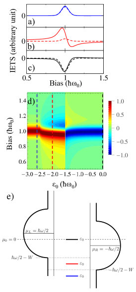
Figure 1: (color online) (a-c) IETS spectrum from LOE (solid) and LOE-WBA (dashed) for three different position of an electronic level, coupling with a wide $s$ band with constant density of states, and a narrow $d$ band with bandwidth $W$ centered at the equilibrium Fermi level $\mu_{0}=0$. (a) $\varepsilon_{0}=-2.6$, (b) $\varepsilon_{0}=-2$, (c) $\varepsilon_{0}=0$. The transmission coefficients at the Fermi level are $T=0.006,0.01,1$, respectively. (d) Contour plot of the IETS spectrum for different level positions. The signal is normalized such that for each given $\varepsilon_{0}$, the height of the largest peak or dip is 1. Parameters in unit of the vibration energy $\hbar\omega_{0}$: $t^{\prime}=2t=W=2$, $\Gamma_{0}=0.1$, $k_{B}T=0.02$. Here, $t$ is the hopping matrix element of the $d$ band, and $t^{\prime}$ is its coupling to the electronic level. (e) Schematics of the one-level model (shown for the three different level positions) biased at the emission threshold $V=\hbar\omega$.

Simple model. First we use a single-level model to illustrate how the “asymmetric” term contains important information about the energy dependence of the electrode couplings. In the LOE-WBA one always has $\kappa_{\lambda}=0$ for symmetric junctions. This is not the case for the LOE expression Eq. (10). We therefore consider a symmetric junction containing a single electronic level at $\varepsilon_{0}$ (with $\mu_{0}=0$), coupled to a local vibration ($\omega_{0}$), and with energy-dependent electrode coupling rates. Assuming symmetrical potential drop, and using the notations $\Gamma_{l}=\Gamma_{L}(\mu_{L})+\Gamma_{R}(\mu_{L})$ and $\Gamma_{r}=\Gamma_{L}(\mu_{R})+\Gamma_{R}(\mu_{R})$ we can write the “symmetric”,

$$\gamma=-C\left\{\Gamma_{l}^{2}\Gamma_{r}^{2}-\left(4\varepsilon_{0}^{2}-\hbar^{2}\omega_{0}^{2}\right)^{2}\right\},$$ (15)

and “asymmetric” coefficients,

$$\kappa=4C\left(\delta\Gamma\,\varepsilon_{0}+\bar{\Gamma}\,\hbar\omega_{0}\right)\left\{\Gamma_{l}\Gamma_{r}-\left(4\varepsilon_{0}^{2}-\hbar^{2}\omega_{0}^{2}\right)\right\},$$ (16)

where $\delta\Gamma=\Gamma_{l}-\Gamma_{r}$, $\bar{\Gamma}=(\Gamma_{l}+\Gamma_{r})/2$, and $C$ a constant common to $\gamma$ and $\kappa$. In the typical case of transition metal electrodes the coupling can contain contributions both from a wide $s$-band as well as from a narrow $d$-band leading to a significant $\delta\Gamma$ and finite $\kappa$. To model the $s$-band we use a constant $\Gamma_{0}$, and to mimic the coupling (hopping $t^{\prime}$) to a $d$-band we add the self-energy of a semi-infinite 1D chain, with bandwidth $2W$ centered at $\mu_{0}=0$. Figure 1 (a-c) compares the signals calculated from LOE-WBA and LOE for different $\varepsilon_{0}$. For both treatments we observe that the peak in the off-resonance IETS evolves into a dip on-resonance. However, only in the LOE the two regimes are separated by a peak-dip structure close to resonance due to the “asymmetric” $\kappa$, which is enhanced at the onset of the coupling with $d$ band in one electrode. The change in IETS signal with a gate-potential ($\varepsilon_{0}$) is shown in Fig. 1 (d). The features observed at $\varepsilon_{0}=\pm\hbar\omega/2-W$ is associated with the level being resonant with the left/right $d$-band onset, respectively.

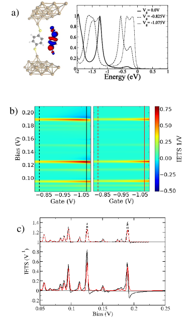
Figure 2: (color online) (a) BDT between two adatoms on Au(111) together with transmission for off resonance (zero gate) and close to resonance. (b) IETS as a function of gate voltage from LOE (left) and LOE-WBA (right). (c) IETS for fixed gate voltage off-resonance (dashed lines, offset for clarity) and close-to-resonance (solid lines). Black: LOE, Red: LOE-WBA. The IETS signals are calculated for $T=4.2$ K and processed to mimic the experimental broadening arising from the lock-in technique with a harmonic voltage modulation of $V_{\mathrm{rms}}=5$ mV Frederiksen et al. (2007).

IETS of benzene-dithiol. It has been possible to apply an external gate potential to junctions with small molecules between metallic electrodes Yu et al. (2004); Song et al. (2009). Under these conditions IETS have been recorded for gated octane-dithiol (ODT) and benzene-dithiol (BDT) molecules between gold electrodes Song et al. (2009). For both ODT and BDT the quite symmetric $I$–$V$ characteristics indicates a symmetric bonding to the electrodes. For the $\pi$-conjugated BDT it was shown how the transport can be tuned from far off-resonance ($G\sim 0.01G_{0}$) to close to the HOMO resonance increasing the conductance by more than an order of magnitude. As in the simple symmetric model above, this was reflected in the shape of the IETS signal for BDT going from a peak for off-resonance, to a peak-dip close to resonance, with the peaks appearing at the same voltages. However, the analysis by Song et al. Song et al. (2009) was based on a model assuming asymmetric electrode couplings at zero bias (STM regime) Persson and Baratoff (1987). Our simple model [Fig. 1(b)] instead suggests that the observed peak-dip lineshape originates solely from the $\Gamma_{l},\Gamma_{r}$ asymmetry driven by the bias voltage near resonance rather than from asymmetric electrode couplings ($\Gamma_{L},\Gamma_{R}$).

Next, we turn to our DFT-NEGF calculations . The importance of an efficient scheme is underlined by the fact that an IETS calculation is required for each gate value. In the break-junction experiments the atomic structure of the junction is unknown. We anticipate that the gap between the electrodes is quite open and involves sharp asperities with low-coordinated gold atoms in order to allow for the external gating to be effective. In order to emulate this, we consider BDT bonded between adatoms on Au(111) surfaces [Fig. 2(a)], and employ only the $\Gamma$-point in the transport calculations yielding sharper features in the electronic structure. We correct the HOMO-LUMO gap García-Suárez and Lambert (2011) and model the electrostatic gating simply by a rigid shift of the molecular orbital energies relative to the gold energies. In Fig. 2(b)-(c) we compare IETS calculated with LOE and LOE-WBA as a function of gating. As in the experiment, we observe three clear signals around $\hbar\omega=95,130,200$ meV due to benzene vibrational modes. Off resonance, the LOE and LOE-WBA are in agreement as expected. But when the gate voltage is tuned to around $V_{g}\approx-1$ V the methods deviate because of the appearance of sharp resonances in the transmission around the Fermi energy [Fig. 2(a)]. These resonances involve the $d$-orbitals on the contacting gold atoms, as seen in the eigenchannel Paulsson and Brandbyge (2007) plot in Fig. 2(a), and result in a peak-dip structure as seen in the experiment and anticipated by the simple model. Thus it is important to go beyond LOE-WBA in order to reproduce the peak to peak-dip transition taken as evidence for close-to-resonance transport.

IETS of alkane-dithiol. As another demonstration of the improvement of LOE over LOE-WBA, we consider molecular junctions formed by straight or tilted butane-dithiol (C4DT) molecules linked via low-coordinated Au adatoms to Au(111) electrodes, see inset to Fig. 3. Based on DFT-NEGF [27] we calculate elastic transmission and IETS for the periodic structure averaged over electron momentum $k_{||}$ Foti et al. . As shown in Fig. 3(a)-(b), transport around the Fermi level is off-resonance but dominated by the tail of a sulfur-derived peak centered at approximately 0.25 eV below the Fermi level. This feature introduces a relatively strong energy-dependence into the electronic structure which makes the WBA questionable. Indeed, as shown in Fig. 3(c), LOE-WBA gives a smaller IETS intensity compared to the LOE for the energetic CH₂ stretch modes ($\hbar\omega\sim 375$ meV). The WBA may thus be the reason why LOE-WBA calculations was reported to underestimate the IETS intensity for these energetic modes in comparison with experiments Okabayashi et al. (2010). We note that the intensity enhancement is found to be more pronounced for the straight configuration, which may be rationalized from Eq. (15) (the condition $\varepsilon_{0}=\pm\hbar\omega_{0}/2$ better describes the vertical than the tilted case). The intensity change reported in Fig. 3 thus suggests the relevance of going beyond LOE-WBA for simulations involving high-energy vibrational modes.

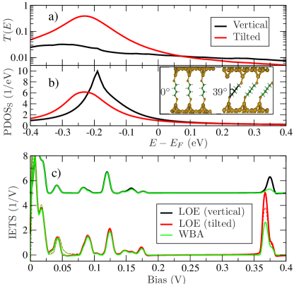
Figure 3: (color online) (a) Transmission and (b) projected density of states over S for vertical and tilted C4DT in a $2\times 2$ supercell of Au(111). (c) IETS within LOE and LOE-WBA (averaged over $k_{||}$) using $T=4.2$ K and $V_{\mathrm{rms}}=5$ mV Frederiksen et al. (2007). Thin dashed lines represent the reverse bias polarity.

Conclusions. A generalized LOE scheme for IETS simulations with the DFT-NEGF method has been described. Without introducing the WBA, our formulation retains both the transparency and computational efficiency of the LOE-WBA. This improvement is important to capture correctly the IETS lineshape in situations where the electronic structure varies appreciably on the scale of the vibration energies, such as near sharp resonances or band edges. Together with DFT-NEGF calculations we have discovered that the intricate experimental lineshape of a gated BDT can be explained without the need to assume asymmetric bonding of the molecule to the electrodes. Also, simulations for C4DT junctions suggest that going beyond WBA is important to capture the IETS intensity related to energetic CH₂ stretch modes.

We acknowledge computer resources from the DCSC. JTL acknowledges support from the National Natural Science Foundation of China (Grant No. 11304107, 61371015), and the Fundamental Research Funds for the Central Universities (HUST:2013TS032). GF and TF acknowledge support from the Basque Departamento de Educacíon and the UPV/EHU (Grant No. IT-756-13), the Spanish Ministerio de Economía y Competitividad (Grant No. FIS2010-19609-CO2-00), and the European Union Integrated Project PAMS.

References

- Stipe et al. (1998) B. C. Stipe, M. A. Rezaei, and W. Ho, Science 280, 1732 (1998).
- Agrait et al. (2002) N. Agrait, C. Untiedt, G. Rubio-Bollinger, and S. Vieira, Phys. Rev. Lett. 88, 216803 (2002).
- Smit et al. (2002) R. H. M. Smit, Y. Noat, C. Untiedt, N. D. Lang, M. C. van Hemert, and J. M. van Ruitenbeek, Nature (London) 419, 906 (2002).
- Kushmerick et al. (2004) J. G. Kushmerick, J. Lazorcik, C. H. Patterson, R. Shashidhar, D. S. Seferos, and G. C. Bazan, Nano Lett. 4, 639 (2004).
- Yu et al. (2004) L. H. Yu, Z. K. Keane, J. W. Ciszek, L. Cheng, M. P. Stewart, J. M. Tour, and D. Natelson, Phys. Rev. Lett. 93, 266802 (2004).
- Song et al. (2009) H. Song, Y. Kim, Y. H. Jang, H. Jeong, M. A. Reed, and T. Lee, Nature 462, 1039 (2009).
- Okabayashi et al. (2013) N. Okabayashi, M. Paulsson, and T. Komeda, Prog. Surf. Sci. 88, 1 (2013).
- Galperin et al. (2007) M. Galperin, M. A. Ratner, and A. Nitzan, J. Phys.: Condens. Matter 19, 103201 (2007).
- Sergueev et al. (2005) N. Sergueev, D. Roubtsov, and H. Guo, Phys. Rev. Lett. 95, 146803 (2005).
- Paulsson et al. (2005) M. Paulsson, T. Frederiksen, and M. Brandbyge, Phys. Rev. B 72, 201101 (2005).
- Jiang et al. (2005) J. Jiang, M. Kula, W. Lu, and Y. Luo, Nano Lett. 5, 1551 (2005).
- Solomon et al. (2006) G. C. Solomon, A. Gagliardi, A. Pecchia, T. Frauenheim, A. Di Carlo, J. R. Reimers, and H. S. Hush, J. Chem. Phys. 124, 094704 (2006).
- Frederiksen et al. (2007) T. Frederiksen, M. Paulsson, M. Brandbyge, and A.-P. Jauho, Phys. Rev. B 75, 205413 (2007).
- Rossen et al. (2013) E. T. R. Rossen, C. F. J. Flipse, and J. I. Cerdá, Phys. Rev. B 87, 235412 (2013).
- Viljas et al. (2005) J. K. Viljas, J. C. Cuevas, F. Pauly, and M. Hafner, Phys. Rev. B 72, 245415 (2005).
- Persson and Baratoff (1987) B. N. J. Persson and A. Baratoff, Phys. Rev. Lett. 59, 339 (1987).
- Egger and Gogolin (2008) R. Egger and A. O. Gogolin, Phys. Rev. B 77, 113405 (2008).
- Okabayashi et al. (2010) N. Okabayashi, M. Paulsson, H. Ueba, Y. Konda, and T. Komeda, Nano Lett. 10, 2950 (2010).
- Haupt et al. (2010) F. Haupt, T. Novotny, and W. Belzig, Phys. Rev. B 82, 165441 (2010).
- Bevilacqua (2013) G. Bevilacqua (2013), arXiv:1303.6206 [math-ph].
- García-Suárez and Lambert (2011) V. M. García-Suárez and C. J. Lambert, New Journal of Physics 13, 053026 (2011).
- Paulsson and Brandbyge (2007) M. Paulsson and M. Brandbyge, Phys. Rev. B 76, 115117 (2007).
- (23) G. Foti, D. Sanchez-Portal, A. Arnau, and T. Frederiksen, (in preparation).
- Soler et al. (2002) J. M. Soler, E. Artacho, J. D. Gale, A. Garcia, J. Junquera, P. Ordejon, and D. Sanchez-Portal, J. Phys.: Condens. Matter 14, 2745 (2002).
- Brandbyge et al. (2002) M. Brandbyge, J. L. Mozos, P. Ordejon, J. Taylor, and K. Stokbro, Phys. Rev. B 65, 165401 (2002).
- Perdew et al. (1996) J. P. Perdew, K. Burke, and M. Ernzerhof, Phys. Rev. Lett. 77, 3865 (1996).