Interactive Sensing in Social Networks

Abstract

This paper presents models and algorithms for interactive sensing in social networks where individuals act as sensors and the information exchange between individuals is exploited to optimize sensing. Social learning is used to model the interaction between individuals that aim to estimate an underlying state of nature. In this context the following questions are addressed: How can self-interested agents that interact via social learning achieve a tradeoff between individual privacy and reputation of the social group? How can protocols be designed to prevent data incest in online reputation blogs where individuals make recommendations? How can sensing by individuals that interact with each other be used by a global decision maker to detect changes in the underlying state of nature? When individual agents possess limited sensing, computation and communication capabilities, can a network of agents achieve sophisticated global behavior? Social and game theoretic learning are natural settings for addressing these questions. This article presents an overview, insights and discussion of social learning models in the context of data incest propagation, change detection and coordination of decision making.

I Introduction and Motivation

The proliferation of social media such as real time microblogging services (Twitter), online reputation and rating systems (YELP) together with app-enabled smartphones, facilitate real time sensing of social activities, social patterns and behavior.

Social sensing, also called participatory sensing [1, 2, 3, 4], is defined as a process where physical sensors present in mobile devices such as GPS are used to infer social relationships and human activities. In this paper, we work at a higher level of abstraction. We use the term social sensor or human-based sensor to denote an agent that provides information about its environment (state of nature) on a social network after interaction with other agents. Examples of such social sensors include Twitter posts, Facebook status updates, and ratings on online reputation systems like YELP and Tripadvisor. Such social sensors go beyond physical sensors for social sensing. For example [5], user opinions/ratings (such as the quality of a restaurant) are available on Tripadvisor but are difficult to measure via physical sensors. Similarly, future situations revealed by the Facebook status of a user are impossible to predict using physical sensors.

Statistical inference using social sensors is relevant in a variety of applications including localizing special events for targeted advertising [6, 7], marketing [8], localization of natural disasters [9] and predicting sentiment of investors in financial markets [10, 11]. It is demonstrated in [12] that models built from the rate of tweets for particular products can outperform market-based predictors. However, social sensors present unique challenges from a statistical estimation point of view. First, social sensors interact with and influence other social sensors. For example, ratings posted on online reputation systems strongly influence the behaviour of individuals. Such interacting sensing can result in non-standard information patterns due to correlations introduced by the structure of the underlying social network. Second, due to privacy reasons and time-constraints, social sensors typically do not reveal raw observations of the underlying state of nature. Instead, they reveal their decisions (ratings, recommendations, votes) which can be viewed as a low resolution (quantized) function of their raw measurements and interactions with other social sensors.

As is apparent from the above discussion, there is strong motivation to construct mathematical models that capture the dynamics of interactive sensing involving social sensors. Such models facilitate understanding the dynamics of information flow in social networks and therefore the design of algorithms that can exploit these dynamics to estimate the underlying state of nature.

In this paper, social learning [15, 16, 17] serves as a useful mathematical abstraction for modelling the interaction of social sensors. Social learning in multi-agent systems seeks to answer the following question:

How do decisions made by agents affect decisions made by subsequent agents?

In social learning, each agent chooses its action by optimizing its local utility function. Subsequent agents then use their private observations together with the actions of previous agents to estimate (learn) an underlying state. The setup is fundamentally different to classical signal processing in which sensors use noisy observations to compute estimates - in social learning agents use noisy observations together with decisions made by previous agents, to estimate the underlying state of nature.

In the last decade, social learning has been used widely in economics, marketing, political science and sociology to model the behavior of financial markets, crowds, social groups and social networks; see [15, 16, 18, 17, 19, 20] and numerous references therein. Related models have been studied in the context of sequential decision making in information theory [21, 22] and statistical signal processing [23, 24] in the electrical engineering literature.

Social learning models for interactive sensing can predict unusual behavior. Indeed, a key result in social learning of an underlying random variable is that rational agents eventually herd [16], that is, they eventually end up choosing the same action irrespective of their private observations. As a result, the actions contain no information about the private observations and so the Bayesian estimate of the underlying random variable freezes. For a multi-agent sensing system, such behavior can be undesirable, particularly if individuals herd and make incorrect decisions.

Main Results and Organization

In the context of social learning models for interactive sensing, the main ideas and organization of this paper are as follows:

1. Social Learning Protocol: Sec.II presents a formulation and survey of the classical Bayesian social learning model which forms the mathematical basis for modelling interactive sensing amongst humans. We illustrate the social learning model in the context of Bayesian signal processing (for easy access to an electrical engineering audience). We then address how self-interested agents performing social learning can achieve useful behavior in terms of optimizing a social welfare function. Such problems are motivated by privacy issues in sensing. If an agent reveals less information in its decisions, it maintains its privacy; on the other hand as part of a social group it has an incentive to optimize a social welfare function that helps estimate the state of nature.
2. Data Incest in Online Reputation Systems: Sec.III deals with the question: How can data incest (misinformation propagation) be prevented in online reputation blogs where social sensors make recommendations?

In the classical social learning model, each agent acts once in a pre-determined order. However, in online reputation systems such as Yelp or Tripadvisor which maintain logs of votes (actions) by agents, social learning takes place with information exchange over a loopy graph (where the agents form the vertices of the graph). Due to the loops in the information exchange graph, data incest (mis-information) can propagate: Suppose an agent wrote a poor rating of a restaurant on a social media site. Another agent is influenced by this rating, visits the restaurant, and then also gives a poor rating on the social media site. The first agent visits the social media site and notices that another agent has also given the restaurant a poor rating - this double confirms her rating and she enters another poor rating.

In a fair reputation system, such “double counting” or data incest should have been prevented by making the first agent aware that the rating of the second agent was influenced by her own rating. Data incest results in a bias in the estimate of state of nature. How can automated protocols be designed to prevent data incest and thereby maintain a fair online reputation system? Sec.III describes how the administrator of a social network can maintain an unbiased (fair) reputation system.
3. Interaction of Local and Global Decision Makers for Change Detection: Sec.IV deals with the question: In sensing where individual agents perform social learning to estimate an underlying state of nature, how can changes in the state of nature be detected? Sec.IV considers a sensing problem that involves change detection. Such sensing problems arise in a variety of applications such as financial trading where individuals react to financial shocks [25]; marketing and advertising [26, 27] where consumers react to a new product; and localization of natural disasters (earthquake and typhoons) [9].

For example, consider measurement of the adoption of a new product using a micro-blogging platform like twitter. The adoption of the technology diffuses through the market but its effects can only be observed through the tweets of select members of the population. These selected members act as sensors for the parameter of interest. Suppose the state of nature suddenly changes due to a sudden market shock or presence of a new competitor. Based on the local actions of the multi-agent system that is performing social learning, a global decision maker (such as a market monitor or technology manufacturer) needs to decide whether or not to declare if a change has occurred. How can the global decision maker achieve such change detection to minimize a cost function comprised of false alarm rate and delay penalty? The local and global decision makers interact, since the local decisions determine the posterior distribution of subsequent agents which determines the global decision (stop or continue) which determines subsequent local decisions. We show that this social learning based change detection problem leads to unusual behavior. The optimal decision policy of the stopping time problem has multiple thresholds. This is unusual: if it is optimal to declare that a change has occurred based on the posterior probability of change, it may not be optimal to declare a change when the posterior probability of change is higher!
4. Coordination of Decisions as a Non-cooperative Game: No discussion on social learning would be complete without mentioning game-theoretic methods. A large body of research on social networks has been devoted to the diffusion of information (e.g., ideas, behaviors, trends) [28, 29], and particularly on finding a set of target nodes so as to maximize the spread of a given product [30, 31]. Often customers end up choosing a specific product among several competitors. A natural approach to model this competitive process is via the use of non-cooperative game theory [32, 33].

Game theory has traditionally been used in economics and social sciences with a focus on fully rational interactions where strong assumptions are made on the information patterns available to individual agents. In comparison, social sensors are agents with partial information and it is the dynamic interactions between agents that is of interest. This motivates the need for game theoretic learning models for agents interacting in social networks.

Sec.V deals with the question: When individuals are self-interested and possess limited sensing, computation and communication capabilities, can a network (social group) of sensors whose utility functions interact achieve sophisticated global behavior? In Sec.V, we discuss a non-cooperative game theoretic learning approach for adaptive decision making in social networks. This can be viewed as a non-Bayesian version of social learning, The aim is to ensure that all agents eventually choose actions from a common polytope of randomized strategies - namely, the set of correlated equilibria of a non-cooperative game. Correlated equilibria are a generalization of Nash equilibria and were introduced by Aumann [34].

Perspective

The social learning and game-theoretic learning formalisms mentioned above can be used either as descriptive tools, to predict the outcome of complex interactions amongst agents in sensing, or as prescriptive tools, to design social networks and sensing systems around given interaction rules. Information aggregation, misinformation propagation and privacy are important issues in sensing using social sensors. In this paper, we treat these issues in a highly stylized manner so as to provide easy accessibility to an electrical engineering audience. The underlying tools used in this paper are widely used by the electrical engineering research community in the areas of signal processing, control, information theory and network communications.

In Bayesian estimation, the twin effects of social learning (information aggregation with interaction amongst agents) and data incest (misinformation propagation) lead to non-standard information patterns in estimating the underlying state of nature. Herding occurs when the public belief overrides the private observations and thus actions of agents are independent of their private observations. Data incest results in bias in the public belief as a consequence of the unintentional re-use of identical actions in the formation of public belief in social learning; the information gathered by each agent is mistakenly considered to be independent. This results in overconfidence and bias in estimates of the state of nature.

Privacy issues impose important constraints on social sensors. Typically, individuals are not willing to disclose private observations. Optimizing interactive sensing with privacy constraints is an important problem. Privacy and trust pose conflicting requirements on human-based sensing: privacy requirements result in noisier measurements or lower resolution actions, while maintaining a high degree of trust (reputation) requires accurate measurements. Utility functions, noisy private measurements and quantized actions are essential ingredients of the social and game-theoretic learning models presented in this paper that facilitate modelling this tradeoff between reputation and privacy.

The literature in the areas of social learning, sensing and networking is extensive. Due to page restrictions, in each of the following sections, we provide only a brief review of relevant works. Seminal books in social networks include [35, 36]. The book [17] contains a complete treatment of social learning models with several remarkable insights. For further references, we refer the reader to [37, 38, 39, 40, 41]. In [42], a nice description is given of how, if individual agents deploy simple heuristics, the global system behavior can achieve ”rational” behavior. The related problem of achieving coherence (i.e., agents eventually choosing the same action or the same decision policy) among disparate sensors of decision agents without cooperation has also witnessed intense research; see [43] and [44]. Non-Bayesian social learning models are also studied in [45, 46].

II Multi-agent Social Learning

This section starts with a brief description of the classical social learning model. In this paper, we use social learning as the mathematical basis for modelling interaction of social sensors. A key result in social learning is that rational agents eventually herd, that is, they pick the same action irrespective of their private observation and social learning stops. To delay the effect of herding, and thereby enhance social learning, Chamley [17] (see also [47] for related work) has proposed a novel constrained optimal social learning protocol. We review this protocol which is formulated as a sequential stopping time problem. We show that the constrained optimal social learning proposed by Chamley [17] has a threshold switching curve in the space of public belief states. Thus the global decision to stop can be implemented efficiently in a social learning model.

II-A Motivation: What is social learning?

We start with a brief description of the ‘vanilla’ social learning model. In social learning [17], agents estimate the underlying state of nature not only from their local measurements, but also from the actions of previous agents. (These previous actions were taken by agents in response to their local measurements; therefore these actions convey information about the underlying state). As we will describe below, the state estimation update in social learning has a drastically different structure compared to the standard optimal filtering recursion and can result in unusual behavior.

Consider a countable number of agents performing social learning to estimate the state of an underlying finite state Markov chain $x$. Let $\mathbb{X}=\{1,2,\ldots,X\}$ denote a finite state space, $P$ the transition matrix and $\pi_{0}$ the initial distribution of the Markov chain.

Each agent acts once in a predetermined sequential order indexed by $k=1,2,\ldots$ The index $k$ can also be viewed as the discrete time instant when agent $k$ acts. A multi-agent system seeks to estimate $x_{0}$. Assume at the beginning of iteration $k$, all agents have access to the public belief $\pi_{k-1}$ defined in Step (iv) below. The social learning protocol proceeds as follows [16, 17]:
(i) Private Observation: At time $k$, agent $k$ records a private observation $y_{k}\in\mathbb{Y}$ from the observation distribution $B_{iy}=P(y|x=i)$, $i\in\mathbb{X}$. Throughout this section we assume that $\mathbb{Y}=\{1,2,\ldots,Y\}$ is finite.
(ii) Private Belief: Using the public belief $\pi_{k-1}$ available at time $k-1$ (defined in Step (iv) below), agent $k$ updates its private posterior belief $\eta_{k}(i)=P(x_{k}=i|a_{1},\ldots,a_{k-1},y_{k})$ as the following Bayesian update (this is the classical Hidden Markov Model filter [48]):

$$\eta_{k} =\frac{B_{y_{k}}P^{\prime}\pi}{\mathbf{1}_{X}^{\prime}B_{y}P^{\prime}\pi},\quad B_{y_{k}}=\text{diag}(P(y_{k}|x=i),i\in\mathbb{X}).$$ (1)

Here $\mathbf{1}_{X}$ denotes the $X$-dimensional vector of ones, $\eta_{k}$ is an $X$-dimensional probability mass function (pmf) and $P^{\prime}$ denotes transpose of the matrix $P$.
(iii) Myopic Action: Agent $k$ takes action $a_{k}\in\mathcal{A}=\{1,2,\ldots,A\}$ to minimize its expected cost

$$a_{k}=\arg\min_{a\in\mathcal{A}}\mathbf{E}\{c(x,a)|a_{1},\ldots,a_{k-1},y_{k}\}\\ =\arg\min_{a\in\mathcal{A}}\{c_{a}^{\prime}\eta_{k}\}.$$ (2)

Here $c_{a}=(c(i,a),i\in\mathbb{X})$ denotes an $X$ dimensional cost vector, and $c(i,a)$ denotes the cost incurred when the underlying state is $i$ and the agent chooses action $a$.
Agent $k$ then broadcasts its action $a_{k}$ to subsequent agents.
(iv) Social Learning Filter: Given the action $a_{k}$ of agent $k$, and the public belief $\pi_{k-1}$, each subsequent agent $k^{\prime}>k$ performs social learning to compute the public belief $\pi_{k}$ according to the following “social learning filter”:

$$\pi_{k}=T(\pi_{k-1},a_{k}),\text{ where }T(\pi,a)=\frac{R^{\pi}_{a}P^{\prime}\pi}{\sigma(\pi,a)},$$ (3)

and $\sigma(\pi,a)=\mathbf{1}_{X}^{\prime}R^{\pi}_{a}P^{\prime}\pi$ is the normalization factor of the Bayesian update. In (3), the public belief $\pi_{k}(i)=P(x_{k}=i|a_{1},\ldots a_{k})$ and $R^{\pi}_{a}=\text{diag}(P(a|x=i,\pi),i\in\mathbb{X})$ has elements

$$P(a_{k}=a|x_{k}=i,\pi_{k-1}=\pi)=\sum_{y\in\mathbb{Y}}P(a|y,\pi)P(y|x_{k}=i)$$ (4)

$$P(a_{k}=a|y,\pi)=\begin{cases}1\text{ if }c_{a}^{\prime}B_{y}P^{\prime}\pi\leq c_{\tilde{a}}^{\prime}B_{y}P^{\prime}\pi,\;\tilde{a}\in\mathcal{A}\\ 0\text{ otherwise. }\end{cases}$$

The derivation of the social learning filter (3) is given in the discussion below.

Figure 1: Information Exchange Structure in Social Learning

II-B Discussion

Let us pause to give some intuition about the above social learning protocol.
1. Information Exchange Structure: Fig.1 illustrates the above social learning protocol in which the information exchange is sequential. Agents send their hard decisions (actions) to subsequent agents. In the social learning protocol we have assumed that each agent acts once. Another way of viewing the social learning protocol is that there are finitely many agents that act repeatedly in some pre-defined order. If each agent chooses its local decision using the current public belief, then the setting is identical to the social learning setup. We also refer the reader to [18] for several recent results in social learning over several types of network adjacency matrices.
2. Filtering with Hard Decisions: Social learning can be viewed as agents making hard decision estimates at each time and sending these estimates to subsequent agents. In conventional Bayesian state estimation, a soft decision is made, namely, the posterior distribution (or equivalently, observation) is sent to subsequent agents. For example, if $\mathcal{A}=\mathbb{X}$, and the costs are chosen as $c_{a}=-e_{a}$ where $e_{a}$ denotes the unit indicator with $1$ in the $a$-th position, then $\operatorname{argmin}_{a}c_{a}^{\prime}\pi=\operatorname{argmax}_{a}\pi(a)$, i.e., the maximum aposteriori probability (MAP) state estimate. For this example, social learning is equivalent to agents sending the hard MAP estimates to subsequent agents.

Note that rather than sending a hard decision estimate, if each agent chooses its action $a_{k}=y_{k}$ (that is agents send their private observations), then the right-hand side of (4) becomes $\sum_{y\in\mathbb{Y}}I(y=y_{k})P(y|x_{k}=i)=P(y_{k}|x_{k}=i)$ and so the problem becomes a standard Bayesian filtering problem.
4. Dependence of Observation Likelihood on Prior: The most unusual feature of the above protocol (to a signal processing audience) is the social learning filter (3). In standard state estimation via a Bayesian filter, the observation likelihood given the state is completely parametrized by the observation noise distribution and is functionally independent of the current prior distribution. In the social learning filter, the likelihood of the action given the state (which is denoted by $R^{\pi}_{a}$) is an explicit function of the prior $\pi$! Not only does the action likelihood depend on the prior, but it is also a discontinuous function, due to the presence of the $\operatorname{argmin}$ in (2).
5. Derivation of Social Learning Filter: The derivation of the social learning filter (3) is as follows: Define the posterior as ${\pi}_{k}(j)=P(x_{k}=j|a_{1},\ldots,a_{k})$. Then

$${\pi}_{k}(j) =\frac{1}{\sigma(\pi_{k-1},a_{k})}P(a_{k}|x_{k}=j,a_{1},\ldots,a_{k-1})$$

$$\sum_{i}P(x_{k}=j|x_{k-1}=i)P(x_{k-1}=i|a_{1},\ldots,a_{k-1})$$

$$=\frac{1}{\sigma(\pi_{k-1},a_{k})}\sum_{y}P(a_{k}|y_{k}=y,a_{1},\ldots,a_{k-1})$$

$$P(y_{k}=y|x_{k}=j)\sum_{i}P(x_{k}=j|x_{k-1}=i){\pi}_{k-1}(i)$$

$$=\frac{1}{\sigma(\pi_{k-1},a_{k})}\sum_{y}P(a_{k}|y_{k}=y,\pi_{k-1})$$

$$\hskip 28.45274ptP(y_{k}=y|x_{k}=j)\sum_{i}P_{ij}{\pi}_{k-1}(i)$$

where the normalization term is

$$\sigma(\pi_{k-1},a_{k})=\sum_{j}\sum_{y}P(a_{k}|y_{k}=y,\pi_{k-1})\\ P(y_{k}=y|x_{k}=j)\sum_{i}P_{ij}{\pi}_{k-1}(i).$$

The above social learning protocol and social learning filter (3) result in interesting dynamics in state estimation and decision making. We will illustrate two interesting consequences that are unusual to an electrical engineering audience:

• Rational Agents form herds and information cascades and blindly follow previous agents. This is discussed in Sec.II-C below.

• Making global decisions on change detection in a multi-agent system performing social learning results in multi-threshold behavior. This is discussed in Sec.IV below.

II-C Rational Agents form Information Cascades

The first consequence of the unusual nature of the social learning filter (3) is that social learning can result in multiple rational agents taking the same action independently of their observations. To illustrate this behavior, throughout this subsection, we assume that $x$ is a finite state random variable (instead of a Markov chain) with prior distribution $\pi_{0}$.

We start with the following definitions; see also [17]:

• An individual agent $k$ herds on the public belief $\pi_{k-1}$ if it chooses its action $a_{k}=a(\pi_{k-1},y_{k})$ in (2) independently of its observation $y_{k}$.

• A herd of agents takes place at time $\bar{k}$, if the actions of all agents after time $\bar{k}$ are identical, i.e., $a_{k}=a_{\bar{k}}$ for all time $k>\bar{k}$.

• An information cascade occurs at time $\bar{k}$, if the public beliefs of all agents after time $\bar{k}$ are identical, i.e. $\pi_{k}=\pi_{\bar{k}}$ for all $k<\bar{k}$.

Note that if an information cascade occurs, then since the public belief freezes, social learning ceases. Also from the above definitions it is clear that an information cascade implies a herd of agents, but the reverse is not true; see Sec.IV-C for an example.

The following result which is well known in the economics literature [16, 17] states that if agents follow the above social learning protocol, then after some finite time $\bar{k}$, an information cascade occurs. The proof follows via an elementary application of the martingale convergence theorem.

Theorem II.1 ([16])

The social learning protocol described in Sec.II-A leads to an information cascade in finite time with probability 1. That is there exists a finite time $\bar{k}$ after which social learning ceases, i.e., public belief $\pi_{k+1}=\pi_{k}$, $k\geq\bar{k}$, and all agents choose the same action, i.e., $a_{k+1}=a_{k}$, $k\geq\bar{k}$. ∎

Instead of reproducing the proof, let us give some insight as to why Theorem II.1 holds. It can be shown using martingale methods that at some finite time $k=k^{*}$, the agent’s probability $P(a_{k}|y_{k},\pi_{k-1})$ becomes independent of the private observation $y_{k}$. Then clearly from (4), $P(a_{k}=a|x_{k}=i,\pi_{k-1})=P(a_{k}=a|\pi)$. Substituting this into the social learning filter (3), we see that $\pi_{k}=\pi_{k-1}$. Thus after some finite time $k^{*}$, the social learning filter hits a fixed point and social learning stops. As a result, all subsequent agents $k>k^{*}$ completely disregard their private observations and take the same action $a_{k^{*}}$, thereby forming an information cascade (and therefore a herd).

II-D Constrained Interactive Sensing: Individual Privacy vs Group Reputation

The above social learning protocol can be interpreted as follows. Agents seek to estimate an underlying state of nature but reveal their actions by maximizing their privacy according to the optimization (2). This leads to an information cascade and social learning stops. In other words, agents are interested in optimizing their own costs (such as maximizing privacy) and ignore the information benefits their action provides to others.

II-D1 Partially Observed Markov Decision Process Formulation

We now describe an optimized social learning procedure that delays herding. This approach, see [17] for an excellent discussion, is motivated by the following question: How can agents assist social learning by choosing their actions to trade off individual privacy (local costs) with optimizing the reputation of the entire social group?

Suppose agents seek to maximize the reputation of their social group by minimizing the following social welfare cost involving all agents in the social group (compared to the myopic objective (2) used in standard social learning):

$$J_{\mu}(\pi_{0})=\mathbf{E}^{\mu}_{\pi_{0}}\biggl{\{}\sum_{k=1}^{\infty}\rho^{k-1}c_{a(\pi_{k-1},y_{k},\mu(\pi_{k-1}))}^{\prime}\eta_{k}\biggr{\}}$$ (5)

In (5), $a(\pi,y,\mu(\pi)))$ denotes the decision rule that agents use to choose their actions as will be explained below. Also $\rho\in[0,1)$ is an economic discount factor and $\pi_{0}$ denotes the initial probability (prior) of the state $x$. $\mathbf{P}^{\mu}_{\pi_{0}}$ and $\mathbf{E}^{\mu}_{\pi_{0}}$ denote the probability measure and expectation of the evolution of the observations and underlying state which are strategy dependent.

The key attribute of (5) is that each agent $k$ chooses its action according to the privacy constrained rule

$$a_{k}=a(\pi_{k-1},y_{k},\mu(\pi_{k-1})).$$ (6)

Here, the policy

$$\mu:\pi_{k-1}\rightarrow\{1,2\ldots,L\}$$

maps the available public belief to the set of $L$ privacy values. The higher the privacy value, the less the agent reveals through its action. This is in contrast to standard social learning (2) in which the action chosen is $a(\pi,y)$, namely a myopic function of the private observation and public belief.

The above formulation can be interpreted as follows: Individual agents seek to maximize their privacy according to social learning (6) but also seek to maximize the reputation of their entire social group (5).

Determining the policy $\mu^{*}$ that minimizes (5), and thereby maximizes the social group reputation, is equivalent to solving a stochastic control problem that is called a partially observed Markov decision process (POMDP) problem [40, 51]. A POMDP comprises of a noisy observed Markov chain and the dynamics of the posterior distribution (belief state) is controlled by a policy ($\mu$ in our case).

II-D2 Structure of Privacy Constrained Sensing Policy

In general, POMDPs are computationally intractable to solve and therefore one cannot say anything useful about the structure of the optimal policy $\mu^{*}$. However, useful insight can be obtained by considering the following extreme case of the above problem. Suppose there are two privacy values and each agent $k$ chooses action

$$a_{k}=\begin{cases}y_{k}&\text{ if }\mu(\pi_{k})=1\text{ (no privacy)}\\ \arg\min_{a}c_{a}^{\prime}\pi_{k-1}&\text{ if }\mu(\pi_{k})=2\text{ (full privacy}).\end{cases}$$

That is, an agent either reveals its raw observation (no privacy) or chooses its action by completely neglecting its observation (full privacy). Once an agent chooses the full privacy option, then all subsequent agents choose exactly the same option and therefore herd - this follows since each agent’s action reveals nothing about the underlying state of nature. Therefore, for this extreme example, determining the optimal policy $\mu^{*}(\pi)$ is equivalent to solving a stopping time problem: Determine the earliest time for agents to herd (maintain full privacy) subject to maximizing the social group reputation.

For such a quickest herding stopping time problem, one can say a lot about the structure of $\mu^{*}(\pi)$. Suppose the sensing system wishes to determine if the state of nature is a specific target state (say state 1). Then [40] shows that under reasonable conditions on the observation distribution and supermodular conditions on the costs ([30] discusses supermodularity of influence in social networks), the dynamic programming recursion has a supermodular structure (see also [52, 53, 54, 41, 55] for related results). This implies that the optimal policy $\mu^{*}$ has the following structure: There exists a threshold curve that partitions the belief space such that when the belief state is on one side of the curve it is optimal for agents to reveal full observations; if the belief state is on the other side of the curve then it is optimal to herd. Moreover, the target state 1 belongs to the region in which it is optimal to herd. This threshold structure of the optimal policy means that if individuals deploy the simple heuristic of

“Choose increased privacy when belief is close to target state” ,

then the group behavior is sophisticated – herding is delayed and accurate estimates of the state of nature can be obtained.

III Data Incest in Online Reputation Systems

This section generalizes the previous section by considering social learning in a social network. How can multiple social sensors interacting over a social network estimate an underlying state of nature? The state could be the position coordinates of an event [9] or the quality of a social parameter such as quality of a restaurant or political party.

The motivation for this section can be understood in terms of the following sensing example. Consider the following interactions in a multi-agent social network where agents seek to estimate an underlying state of nature. Each agent visits a restaurant based on reviews on an online reputation website. The agent then obtains a private measurement of the state (e.g., the quality of food in a restaurant) in noise. After that, he reviews the restaurant on the same online reputation website. The information exchange in the social network is modeled by a directed graph. As mentioned in the introduction, data incest [57] arises due to loops in the information exchange graph. This is illustrated in the graph of Fig.2. Agents 1 and 2 exchange beliefs (or actions) as depicted in Fig.2. The fact that there are two distinct paths between Agent 1 at time 1 and Agent 1 at time 3 (these two paths are denoted in red) implies that the information of Agent 1 at time 1 is double counted thereby leading to a data incest event.

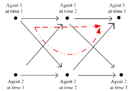
Figure 2: Example of the information flow (communication graph) in a social network with two agents and over three event epochs. The arrows represent exchange of information.

How can data incest be removed so that agents obtain a fair (unbiased) estimate of the underlying state? The methodology of this section can be interpreted in terms of the recent Time article [58] which provides interesting rules for online reputation systems. These include: (i) review the reviewers, and (ii) censor fake (malicious) reviewers. The data incest removal algorithm proposed in this paper can be viewed as “reviewing the reviews” of other agents to see if they are associated with data incest or not.

The rest of this section is organized as follows:

1. Sec.III-A describes the social learning model that is used to mimic the behavior of agents in online reputation systems. The information exchange between agents in the social network is formulated on a family of time dependent directed acyclic graphs.

2. In Sec.III-B, a fair reputation protocol is presented and the criterion for achieving a fair rating is defined.

3. Sec.III-C presents an incest removal algorithm so that the online reputation system achieves a fair rating. A necessary and sufficient condition is given on the graph structure of information exchange between agents so that a fair rating is achievable.

Related works

Collaborative recommendation systems are reviewed and studied in [59, 60]. In [61], a model of Bayesian social learning is considered in which agents receive private information about the state of nature and observe actions of their neighbors in a tree-based network. Another type of mis-information caused by influential agents (agents who heavily affect actions of other agents in social networks) is investigated in [18]. Mis-information in the context of this paper is motivated by sensor networks where the term “data incest” is used [62]. Data incest also arises in Belief Propagation (BP) algorithms [63, 64] which are used in computer vision and error-correcting coding theory. BP algorithms require passing local messages over the graph (Bayesian network) at each iteration. For graphical models with loops, BP algorithms are only approximate due to the over-counting of local messages [65] which is similar to data incest in social learning. With the algorithms presented in this section, data incest can be mitigated from Bayesian social learning over non-tree graphs that satisfy a topological constraint. The closest work to the current paper is [57]. However, in [57], data incest is considered in a network where agents exchange their private belief states - that is, no social learning is considered. Simpler versions of this information exchange process and estimation were investigated in [66, 67, 68].

III-A Information Exchange Graph in Social Network

Consider an online reputation system comprised of social sensors $\{1,2,\ldots,S\}$ that aim to estimate an underlying state of nature (a random variable). Let $x\in\mathbb{X}=\{1,2,\ldots,X\}$ represent the state of nature (such as the quality of a hotel) with known prior distribution $\pi_{0}$. Let $k=1,2,3,\ldots$ depict epochs at which events occur. These events involve taking observations, evaluating beliefs and choosing actions as described below. The index $k$ marks the historical order of events and not necessarily absolute time. However, for simplicity, we refer to $k$ as “time”.

To model the information exchange in the social network, we will use a family of directed acyclic graphs. It is convenient also to reduce the coordinates of time $k$ and agent $s$ to a single integer index $n$ which is used to represent agent $s$ at time $k$:

$$n\triangleq s+S(k-1),\quad s\in\{1,\ldots,S\},\;k=1,2,3,\ldots$$ (7)

We refer to $n$ as a “node” of a time dependent information flow graph $G_{n}$ that we now define.

III-A1 Some Graph Theoretic Definitions

Let

$$G_{n}=(V_{n},E_{n}),\quad n=1,2,\ldots$$ (8)

denote a sequence of time-dependent graphs of information flow in the social network until and including time $k$ where $n=s+S(k-1)$. Each vertex in $V_{n}$ represents an agent $s^{\prime}$ in the social network at time $k^{\prime}$ and each edge $(n^{\prime},n^{\prime\prime})$ in $E_{n}\subseteq V_{n}\times V_{n}$ shows that the information (action) of node $n^{\prime}$ (agent $s^{\prime}$ at time $k^{\prime}$) reaches node $n^{\prime\prime}$ (agent $s^{\prime\prime}$ at time $k^{\prime\prime}$). It is clear that the communication graph $G_{n}$ is a sub-graph of $G_{n+1}$. This means that the diffusion of actions can be modelled via a family of time-dependent directed acyclic graphs (a directed graph with no directed cycles.

The algorithms below will involve specific columns of the adjacency matrix transitive closure matrix of the graph $G_{n}$. The Adjacency Matrix $A_{n}$ of $G_{n}$ is an $n\times n$ matrix with elements $A_{n}(i,j)$ given by

$$A_{n}(i,j)=\begin{cases}1&\textrm{ if }(v_{j},v_{i})\in E\;,\\ 0&\textrm{ otherwise}\end{cases}\;,\text{ }A_{n}(i,i)=0.$$ (9)

The transitive closure matrix $T_{n}$ is the $n\times n$ matrix

$$T_{n}=\text{sgn}((\mathbf{I}_{n}-A_{n})^{-1})$$ (10)

where for any matrix $M$, the matrix $\text{sgn}(M)$ has elements

$$\text{sgn}(M)(i,j)=\begin{cases}0&\text{ if }M(i,j)=0\;,\\ 1&\text{ if }M(i,j)\neq 0.\end{cases}$$

Note that $A_{n}(i,j)=1$ if there is a single hop path between nodes $i$ and $j$, In comparison, $T_{n}(i,j)=1$ if there exists a path (possible multi-hop) between node $i$ and $j$.

The information reaching node $n$ depends on the information flow graph $G_{n}$. The following two sets will be used to specify the incest removal algorithms below:

$$\mathcal{H}_{n} =\{m:A_{n}(m,n)=1\}$$ (11)

$$\mathcal{F}_{n} =\{m:T_{n}(m,n)=1\}.$$ (12)

Thus $\mathcal{H}_{n}$ denotes the set of previous nodes $m$ that communicate with node $n$ in a single-hop. In comparison, $\mathcal{F}_{n}$ denotes the set of previous nodes $m$ whose information eventually arrive at node $n$. Thus $\mathcal{F}_{n}$ contains all possible multi-hop connections by which information from a node $m$ eventually reaches node $n$.

III-A2 Example

To illustrate the above notation consider a social network consisting of $S=2$ two groups with the following information flow graph for three time points $k=1,2,3$.

Figure 3: Example of an information flow network with $S=2$ two agents, namely $s\in\{1,2\}$ and time points $k=1,2,3$. Circles represent the nodes indexed by $n=s+S(k-1)$ in the social network and each edge depicts a communication link between two nodes.

Fig.3 shows the nodes $n=1,2,\ldots,6$ where $n=s+2(k-1)$.

Note that in this example, as is apparent from Fig.2, each node remembers all its previous actions. The information flow is characterized by the family of directed acyclic graphs $\{G_{1},G_{2},G_{3},G_{4},G_{5},G_{6}\}$ with adjacency matrices
$A_{1}=\begin{bmatrix}0\end{bmatrix}$, $A_{2}=\begin{bmatrix}0&0\\ 0&0\end{bmatrix}$, $A_{3}=\begin{bmatrix}0&0&1\\ 0&0&1\\ 0&0&0\end{bmatrix}$,

$$A_{4}=\begin{bmatrix}0&0&1&1\\ 0&0&1&1\\ 0&0&0&0\\ 0&0&0&0\end{bmatrix},\;A_{5}=\begin{bmatrix}0&0&1&1&1\\ 0&0&1&1&1\\ 0&0&0&0&1\\ 0&0&0&0&1\\ 0&0&0&0&0\end{bmatrix}.$$

Since nodes 1 and 2 do not communicate, clearly $A_{1}$ and $A_{2}$ are zero matrices. Nodes 1 and 3 communicate as do nodes 2 and 3, hence $A_{3}$ has two ones, etc. Finally from (11) and (12),

$$\mathcal{H}_{5}=\{1,2,3,4\},\quad\mathcal{F}_{5}=\{1,2,3,4\}$$

where $\mathcal{H}_{5}$ denotes all one hop links to node 5 while $\mathcal{F}_{5}$ denotes all multihop links to node 5.

Note that $A_{n}$ is always the upper left $n\times n$ submatrix of $A_{n+1}$. Also due to causality with respect to the time index $k$, the adjacency matrices are always upper triangular.

III-B Fair Online Reputation System

III-B1 Protocol for Fair Online Reputation System

The procedure summarized in Protocol 1 aims to evaluate a fair reputation that uses social learning over a social network by eliminating incest.

(i) Information from Social Network:

1. Recommendation from friends: Node $n$ receives past actions $\{a_{m},m\in\mathcal{H}_{n}\}$ from previous nodes $m\in\mathcal{H}_{n}$ in the social network. $\mathcal{H}_{n}$ is defined in (11).

2. Automated Recommender System: For these past actions $\{a_{m},m\in\mathcal{H}_{n}\}$, the network administrator has already computed the public beliefs $(\pi_{m},m\in\mathcal{H}_{n})$ using Step (v) below.
   The automated recommender system fuses public beliefs $(\pi_{m},m\in\mathcal{H}_{n})$, into the single recommendation belief ${\pi}_{n-}$ as

   $${\pi}_{n-}=\mathcal{A}(\pi_{m},m\in\mathcal{H}_{n})$$ (13)

   The fusion algorithm $\mathcal{A}$ will be designed below.

(ii) Observation: Node $n$ records private observation $y_{n}$ from distribution $B_{iy}=P(y|x=i)$, $i\in\mathbb{X}$.
(iii) Private Belief: Node $n$ then uses $y_{n}$ and public belief ${\pi}_{n-}$ to update its private belief via Bayes formula as

$$\eta_{n}=\frac{B_{y_{n}}{\pi}_{n-}}{\mathbf{1}_{X}^{\prime}B_{y}{\pi}_{n-}}$$ (14)

(iv) Myopic Action: Node $n$ takes action

$$a_{n}=\arg\min_{a}c_{a}^{\prime}\eta_{n}$$

and inputs its action to the online reputation system.
(v) Public Belief Update by Network Administrator: Based on action $a_{n}$, the network administrator (automated algorithm) computes the public belief $\pi_{n}$ using the social learning filter (3) with $P=I$.

Protocol 1 Incest Removal for Social Learning in an Online Reputation System

Aim: Our aim is to design algorithm $\mathcal{A}$ in the automated recommender system (13) of Protocol 1 so that the following requirement is met:

$${\pi}_{n-}(i) =\pi^{0}_{n-}(i),\quad i\in\mathbb{X}$$

where $$\pi^{0}_{n-}(i)=P(x=i|\{a_{m},m\in\mathcal{F}_{n}\}).$$ (15)

We call $\pi^{0}_{n-}$ in (15) the true or fair online rating available to node $n$ since $\mathcal{F}_{n}=\{m:T_{n}(m,n)=1\}$ defined in (12) denotes all information (multi-hop links) available to node $n$. By definition $\pi^{0}_{n-}$ is incest free since it is the desired conditional probability that we want. If algorithm $\mathcal{A}$ is designed so that ${\pi}_{n-}(i)$ satisfies (15), then the computation (14) and Step (v) yield

$$\eta_{n}(i) =P(x=i|\{a_{m},m\in\mathcal{F}_{n}\},y_{n}),\quad i\in\mathbb{X},$$

$$\pi_{n}(i) =P(x=i|\{a_{m},m\in\mathcal{F}_{n}\},a_{n}),\quad i\in\mathbb{X},$$

which are, respectively, the correct private belief for node $n$ and the correct after-action public belief.

III-B2 Discussion of Protocol 1

(i) Data Incest: It is important to note that without careful design of algorithm $\mathcal{A}$, due to loops in the dependencies of actions on previous actions, the public rating ${\pi}_{n-}$ computed using (13) can be substantially different from the fair online rating $\pi^{0}_{n-}$ of (15). As a result, $\eta_{n}$ computed via (14) will not be the correct private belief and incest will propagate in the network. In other words, $\eta_{n}$, ${\pi}_{n-}$ and ${\pi}_{n}$ are defined purely in terms of their computational expressions in Protocol 1 – at this stage they are not necessarily the desired conditional probabilities, unless algorithm $\mathcal{A}$ is designed to remove incest.

Note that instead of (13), node $n$ could naively (and incorrectly) assume that the public beliefs ${\pi}_{m},m\in\mathcal{H}_{n}$ that it received are independent. It would then fuse these public beliefs as

$${\pi}_{n}{-}=\frac{\sum_{m\in\mathcal{H}_{n}}{\pi}_{m}}{\mathbf{1}_{X}^{\prime}\sum_{m\in\mathcal{H}_{n}}{\pi}_{m}}.$$ (16)

This, of course, would result in data incest.
(ii) How much does an individual remember?: The above protocol has the flexibility of modelling cases where either each node remembers some (or all) of its past actions or none of its past actions. This facilitates modelling cases in which people forget most of the past except for specific highlights.
(iii) Automated Recommender System: Steps (i) and (v) of Protocol 1 can be combined into an automated recommender system that maps previous actions of agents in the social group to a single recommendation (rating) ${\pi}_{n-}$ of (13). This recommender system can operate completely opaquely to the actual user (node $n$). Node $n$ simply uses the automated rating ${\pi}_{n-}$ as the current best available rating from the reputation system.
(iii) Social Influence. Informational Message vs Social Message: In Protocol 1, it is important that each individual $n$ deploys Algorithm $\mathcal{A}$ to fuse the beliefs $\{{\pi}_{m},m\in\mathcal{H}_{n}\}$; otherwise incest can propagate. Here, $\mathcal{H}_{n}$ can be viewed as the “social message”, i.e., personal friends of node $n$ since they directly communicate to node $n$ while the associated beliefs can be viewed as the “informational message”. The social message from personal friends exerts a large social influence – it provides significant incentive (peer pressure) for individual $n$ to comply with Protocol 1 and thereby prevent incest. Indeed, a remarkable recent study described in [69] shows that social messages (votes) from known friends has significantly more influence on an individual than the information in the messages themselves. This study includes comparison of information messages and social messages on Facebook and their direct effect on voting behavior. To quote [69], “The effect of social transmission on real-world voting was greater than the direct effect of the messages themselves…”

(iv) Agent Reputation: The cost function minimization in Step (iv) can be interpreted in terms of the reputation of agents in online reputation systems. If an agent continues to write bad reviews for high quality restaurants on Yelp, his reputation becomes lower among the users. Consequently, other people ignore reviews of that (low-reputation) agent in evaluating their opinion about the social unit under study (restaurant). Therefore, agents minimize the penalty of writing inaccurate reviews (or equivalently increase their reputations) by choosing proper actions.
(v) Think and act: Steps (ii), (iii) (iv) and (v) of Protocol 1 constitute standard social learning as described in Sec.II-A. The key difference with standard social learning is Steps (i) performed by the network administrator. Agents receive public beliefs from the social network with arbitrary random delays. These delays reflect the time an agent takes between reading the publicly available reputation and making its decision. It is typical behavior of people to read published ratings multiple times and then think for an arbitrary amount of time before acting.

III-C Incest Removal Algorithm in Online Reputation System

Below we design algorithm $\mathcal{A}$ in Protocol 1 so that it yields the fair public rating $\pi^{0}_{n-}$ of (15).

III-C1 Fair Rating Algorithm

It is convenient to work with the logarithm of the un-normalized belief; accordingly define

$$l_{n}(i)\propto\log{\pi}_{n}(i),\quad l_{n-}(i)\propto\log{\pi}_{n-}(i),\quad i\in\mathbb{X}.$$

The following theorem shows that the logarithm of the fair rating $\pi^{0}_{n-}$ defined in (15) can be obtained as linear weighted combination of the logarithms of previous public beliefs.

Theorem III.1 (Fair Rating Algorithm)

Consider the online reputation system running Protocol 1. Suppose the following algorithm $\mathcal{A}(l_{m},m\in\mathcal{H}_{n})$ is implemented in (13) of Protocol 1 by the network administrator:

$$l_{n-}(i) =w_{n}^{\prime}\,l_{1:n-1}(i)$$

where $$\;w_{n}=T_{n-1}^{-1}t_{n}.$$ (17)

Then $l_{n-}(i)\propto\log\pi^{0}_{n-}(i)$. That is, algorithm $\mathcal{A}$ computes the fair rating $\log\pi^{0}_{n-}(i)$ defined in (15).
In (III.1), $w_{n}$ is an $n-1$ dimensional weight vector. Recall that $t_{n}$ denotes the first $n-1$ elements of the $n$th column of transitive closure matrix $T_{n}$. ∎

Theorem III.1 says that the fair rating $\pi^{0}_{n-}$ can be expressed as a linear function of the action log-likelihoods in terms of the transitive closure matrix $T_{n}$ of graph $G_{n}$. This is intuitive since $\pi^{0}_{n-}$ can be viewed as the sum of information collected by the nodes such that there are paths between all these nodes and $n$.

III-C2 Achievability of Fair Rating by Protocol 1

We are not quite done!

1. On the one hand, algorithm $\mathcal{A}$ at node $n$ specified by (13) has access only to beliefs $l_{m},m\in\mathcal{H}_{n}$ – equivalently it has access only to beliefs from previous nodes specified by $A_{n}(:,n)$ which denotes the last column of the adjacency matrix $A_{n}$.

2. On the other hand, to provide incest free estimates, algorithm $\mathcal{A}$ specified in (III.1) requires all previous beliefs $l_{1:n-1}(i)$ that are specified by the non-zero elements of the vector $w_{n}$.

The only way to reconcile points 1 and 2 is to ensure that $A_{n}(j,n)=0$ implies $w_{n}(j)=0$ for $j=1,\ldots,n-1$. The condition means that the single hop past estimates $l_{m},m\in\mathcal{H}_{n}$ available at node $n$ according to (13) in Protocol 1 provide all the information required to compute $w_{n}^{\prime}\,l_{1:n-1}$ in (III.1). This is a condition on the information flow graph $G_{n}$. We formalize this condition in the following theorem.

Theorem III.2 (Achievability of Fair Rating)

Consider the fair rating algorithm specified by (III.1). For Protocol 1 with available information $({\pi}_{m},m\in\mathcal{H}_{n})$ to achieve the estimates $l_{n-}$ of algorithm (III.1), a necessary and sufficient condition on the information flow graph $G_{n}$ is

$$A_{n}(j,n)=0\implies w_{n}(j)=0.$$ (18)

Therefore for Protocol 1 to generate incest free estimates for nodes $n=1,2,\ldots$, condition (18) needs to hold for each $n$. (Recall $w_{n}$ is specified in (III.1).) ∎

Note that the constraint (18) is purely in terms of the adjacency matrix $A_{n}$, since the transitive closure matrix (10) is a function of the adjacency matrix.

Summary: Algorithm (III.1) together with the condition (18) ensure that incest free estimates are generated by Protocol 1.

III-C3 Illustrative Example (continued)

Let us continue with the example of Fig.2 where we already specified the adjacency matrices of the graphs $G_{1}$, $G_{2}$, $G_{3}$, $G_{4}$ and $G_{5}$. Using (10), the transitive closure matrices $T_{n}$ obtained from the adjacency matrices are given by:
$T_{1}=\begin{bmatrix}1\end{bmatrix},T_{2}=\begin{bmatrix}1&0\\ 0&1\end{bmatrix},T_{3}=\begin{bmatrix}1&0&1\\ 0&1&1\\ 0&0&1\end{bmatrix}$,
$T_{4}=\begin{bmatrix}1&0&1&1\\ 0&1&1&1\\ 0&0&1&0\\ 0&0&0&1\end{bmatrix},T_{5}=\begin{bmatrix}1&0&1&1&1\\ 0&1&1&1&1\\ 0&0&1&0&1\\ 0&0&0&1&1\\ 0&0&0&0&1\end{bmatrix}$.
Note that $T_{n}(i,j)$ is non-zero only for $i\geq j$ due to causality since information sent by a social group can only arrive at another social group at a later time instant. The weight vectors are then obtained from (III.1) as $\\ w_{2}=\begin{bmatrix}0\end{bmatrix},\;\\ w_{3}=\begin{bmatrix}1&1\end{bmatrix}^{\prime},\;\\ w_{4}=\begin{bmatrix}1&1&0\end{bmatrix}^{\prime},\;\\ w_{5}=\begin{bmatrix}-1&-1&1&1\end{bmatrix}^{\prime}.\\$ Let us examine these weight vectors. $w_{2}$ means that node $2$ does not use the estimate from node $1$. This formula is consistent with the constraint information flow because estimate from node $1$ is not available to node $2$; see Fig.3. $w_{3}$ means that node $3$ uses estimates from node $1$ and $2$; $w_{4}$ means that node $4$ uses estimates only from node $1$ and node $2$. The estimate from node $3$ is not available at node 4. As shown in Fig.3, the mis-information propagation occurs at node $5$. The vector $w_{5}$ says that node 5 adds estimates from nodes $3$ and $4$ and removes estimates from nodes $1$ and $2$ to avoid double counting of these estimates already integrated into estimates from node $3$ and $4$. Indeed, using the algorithm (III.1), incest is completely prevented in this example.

Let us now illustrate an example in which exact incest removal is impossible. Consider the information flow graph of Fig.3 but with the edge between node 2 and node 5 deleted. Then $A_{5}(2,5)=0$ while $w_{5}(2)\neq 0$, and therefore the condition (18) does not hold. Hence exact incest removal is not possible for this case.

III-D Summary

In this section, we have outlined a controlled sensing problem over a social network in which the administrator controls (removes) data incest and thereby maintains an unbiased (fair) online reputation system. The state of nature could be geographical coordinates of an event (in a target localization problem) or quality of a social unit (in an online reputation system). As discussed above, data incest arises due to the recursive nature of Bayesian estimation and non-determinism in the timing of the sensing by individuals. Details of proofs, extensions and further numerical studies are presented in [57, 70].

IV Interactive Sensing for Quickest Change Detection

In this section we consider interacting social sensors in the context of detecting a change in the underlying state of nature. Suppose a multi-agent system performs social learning and makes local decisions as described in Sec.II. Given the public beliefs from the social learning protocol, how can quickest change detection be achieved? In other words, how can a global decision maker use the local decisions from individual agents to decide when a change has occurred? It is shown below that making a global decision (change or no change) based on local decisions of individual agents has an unusual structure resulting in a non-convex stopping set.

A typical application of such social sensors arises in the measurement of the adoption of a new product using a micro-blogging platform like Twitter. The adoption of the technology diffuses through the market but its effects can only be observed through the tweets of select individuals of the population. These selected individuals act as sensors for estimating the diffusion. They interact and learn from the decisions (tweeted sentiments) of other members and therefore perform social learning. Suppose the state of nature suddenly changes due to a sudden market shock or presence of a new competitor. The goal for a market analyst or product manufacturer is to detect this change as quickly as possible by minimizing a cost function that involves the sum of the false alarm and decision delay.

Related works

[26, 27] model diffusion in networks over a random graph with arbitrary degree distribution. The resulting diffusion is approximated using deterministic dynamics via a mean field approach [71]. In the seminal paper [1], a sensing system for complex social systems is presented with data collected from cell phones. This data is used in [1] to recognize social patterns, identify socially significant locations and infer relationships. In [9], people using a microblogging service such as Twitter are considered as sensors. In particular, [9] considers each Twitter user as a sensor and uses a particle filtering algorithm to estimate the centre of earthquakes and trajectories of typhoons. As pointed out in [9], an important characteristic of microblogging services such as Twitter is that they provide real-time sensing – Twitter users tweet several times a day; whereas standard blog users update information once every several days.

Apart from the above applications in real time sensing, change detection in social learning also arises in mathematical finance models. For example, in agent based models for the microstructure of asset prices in high frequency trading in financial systems [25], the state denotes the underlying asset value that changes at a random time $\tau^{0}$. Agents observe local individual decisions of previous agents via an order book, combine these observed decisions with their noisy private signals about the asset, selfishly optimize their expected local utilities, and then make their own individual decisions (whether to buy, sell or do nothing). The market evolves through the orders of trading agents. Given this order book information, the goal of the market maker (global decision maker) is to achieve quickest change point detection when a shock occurs to the value of the asset [72].

IV-A Classical Quickest Detection

The classical Bayesian quickest time detection problem [73] is as follows: An underlying discrete-time state process $x$ jump-changes at a geometrically distributed random time $\tau^{0}$. Consider a sequence of discrete time random measurements $\{y_{k},k\geq 1\}$, such that conditioned on the event $\{\tau^{0}=t\}$, $y_{k}$, $k\leq t$ are independent and identically distributed (i.i.d.) random variables with distribution $B_{1}$ and $y_{k},k>t$ are i.i.d. random variables with distribution $B_{2}$. The quickest detection problem involves detecting the change time $\tau^{0}$ with minimal cost. That is, at each time $k=1,2,\ldots$, a decision $u_{k}\in\{1\text{ (stop and announce change)},2\text{ (continue)}\}$ needs to be made to optimize a tradeoff between false alarm frequency and linear delay penalty.

To formalize this setup, let $P=\begin{bmatrix}1&0\\ 1-P_{22}&P_{22}\end{bmatrix}$ denote the transition matrix of a two state Markov chain $x$ in which state 1 is absorbing. Then it is easily seen that the geometrically distributed change time $\tau^{0}$ is equivalent to the time at which the Markov chain enters state 1. That is $\tau^{0}=\min\{k:x_{k}=1\}$ and $\mathbf{E}\{\tau^{0}\}=1/(1-P_{22})$. Let $\tau$ be the time at which the decision $u_{k}=1$ (announce change) is taken. The goal of quickest time detection is to minimize the Kolmogorov–Shiryaev criterion for detection of a disorder [74]:

$$J_{\mu}(\pi_{0})=d\,\mathbf{E}^{\mu}_{\pi_{0}}\{(\tau-\tau^{0})^{+}\}+f\mathbf{P}^{\mu}_{\pi_{0}}(\tau<\tau^{0}).$$ (19)

Here $x^{+}=x$ if $x\geq 0$ and $0$ otherwise. The non-negative constants $d$ and $f$ denote the delay and false alarm penalties, respectively. So waiting too long to announce a change incurs a delay penalty $d$ at each time instant after the system has changed, while declaring a change before it happens, incurs a false alarm penalty $f$. In (19) $\mu$ denotes the strategy of the decision maker. $\mathbf{P}^{\mu}_{\pi_{0}}$ and $\mathbf{E}^{\mu}_{\pi_{0}}$ are the probability measure and expectation of the evolution of the observations and Markov state which are strategy dependent. $\pi_{0}$ denotes the initial distribution of the Markov chain $x$.

In classical quickest detection, the decision policy $\mu$ is a function of the two-dimensional belief state (posterior probability mass function) $\pi_{k}(i)=P(x_{k}=i|y_{1},\ldots,y_{k},u_{1},\ldots,u_{k-1})$, $i=1,2$, with $\pi_{k}(1)+\pi_{k}(2)=1$. So it suffices to consider one element, say $\pi_{k}(2)$, of this probability mass function. Classical quickest change detection (see for example [73]) says that the policy $\mu^{*}(\pi)$ which optimizes (19) has the following threshold structure: There exists a threshold point $\pi^{*}\in[0,1]$ such that

$$\mu^{*}(\pi_{k})=\begin{cases}2\text{ (continue) }&\text{ if }\pi_{k}(2)\geq\pi^{*}\\ 1\text{ (announce change) }&\text{ if }\pi_{k}(2)<\pi^{*}.\end{cases}$$ (20)

IV-B Multi-agent Quickest Detection Problem

With the above classical formulation in mind, consider now the following multi-agent quickest change detection problem. Suppose that a multi-agent system performs social learning to estimate an underlying state according to the social learning protocol of Sec.II-A. That is, each agent acts once in a predetermined sequential order indexed by $k=1,2,\ldots$ (Equivalently, as pointed out in the discussion in Sec.II-A, a finite number of agents act repeatedly in some pre-defined order and each agent chooses its local decision using the current public belief.) Given these local decisions (or equivalently the public belief), the goal of the global decision maker is to minimize the quickest detection objective (19). The problem now is a non-trivial generalization of classical quickest detection. The posterior $\pi$ is now the public belief given by the social learning filter (3) instead of a standard Bayesian filter. There is now interaction between the local and global decision makers. The local decision $a_{k}$ from the social learning protocol determines the public belief state $\pi_{k}$ via the social learning filter (3), which determines the global decision (stop or continue), which determines the local decision at the next time instant, and so on.

The global decision maker’s policy $\mu^{*}:\pi\rightarrow\{1,2\}$ that optimizes the quickest detection objective (19) and the cost $J_{\mu^{*}}(\pi_{0})$ of this optimal policy are the solution of “Bellman’s dynamic programming equation”

$$\mu^{*}(\pi) =\arg\min\{f\pi(2),\;d(1-\pi(2))$$

$$+\sum_{a\in\mathcal{A}}V\left(T(\pi,a)\right)\sigma(\pi,a)\},\quad J_{\mu^{*}}(\pi_{0})=V(\pi_{0})$$

$$V(\pi) =\min\{f\pi(2),\;d(1-\pi(2))$$

$$\hskip 42.67912pt+\sum_{a\in\mathcal{A}}V\left(T(\pi,a)\right)\sigma(\pi,a)\}.$$ (21)

Here $T(\pi,a)$ and $\sigma(\pi,a)$ are given by the social learning filter (3) - recall that $a$ denotes the local decision. $V(\pi)$ is called the “value function” – it is the cost incurred by the optimal policy when the initial belief state (prior) is $\pi$. As will be shown the numerical example below, the optimal policy $\mu^{*}(\pi)$ has a very different structure compared to classical quickest detection.

IV-C Numerical Example

We now illustrate the unusual multi-threshold property of the global decision maker’s optimal policy $\mu^{*}(\pi)$ in multi-agent quickest detection with social learning. Consider the social learning model of Sec.II-A with the following parameters: The underlying state is a 2-state Markov chain $x$ with state space $\mathbb{X}=\{1,2\}$ and transition probability matrix $P=\begin{bmatrix}1&0\\ 0.05&0.95\end{bmatrix}$. So the change time $\tau^{0}$ (i.e., the time the Markov chain jumps from state 2 into absorbing state 1) is geometrically distributed with $E\{\tau^{0}\}=1/0.05=20$.

Social Learning Parameters: Individual agents observe the Markov chain $x$ in noise with the observation symbol set $\mathbb{Y}=\{1,2\}$. Suppose the observation likelihood matrix with elements $B_{iy}=P(y_{k}=y|x_{k}=i)$ is $B=\begin{bmatrix}0.9&0.1\\ 0.1&0.9\end{bmatrix}$. Agents can choose their local actions $a$ from the action set $\mathcal{A}=\{1,2\}$. The state dependent cost matrix of these actions is $c=(c(i,a),i\in X,a\in\mathcal{A})=\begin{bmatrix}4.57&5.57\\ 2.57&0\end{bmatrix}$. Agents perform social learning with the above parameters. The intervals $[0,\pi_{1}^{*}]$ and $[\pi_{2}^{*},1]$ in Fig.4(a) are regions where the optimal local actions taken by agents are independent of their observations. For $\pi(2)\in[\pi_{2}^{*},1]$, the optimal local action is 2 and for $\pi(2)\in[0,\pi_{1}^{*}]$, the optimal local action is 1. So individual agents herd for belief states in these intervals (see the definition in Sec.II-C) and the local actions do not yield any information about the underlying state. Moreover, the interval $[0,\pi_{1}^{*}]$ depicts a region where all agents herd (again see the definition in Sec.II-C), meaning that once the belief state is in this region, it remains so indefinitely and all agents choose the same local action 1.

Global Decision Making: Based on the local actions of the agents performing social learning, the global decision maker needs to perform quickest change detection. The global decision maker uses the delay penalty $d=1.05$ and false alarm penalty $f=3$ in the objective function (19). The optimal policy $\mu^{*}(\pi)$ of the global decision maker where $\pi=[1-\pi(2),\pi(2)]^{\prime}$ is plotted versus $\pi(2)$ in Fig.4(a). Note $\pi(2)=1$ means that with certainty no change has occurred, while $\pi(2)=0$ means with certainty a change has occurred. The policy $\mu^{*}(\pi)$ was computed by constructing a uniform grid of 1000 points for $\pi(2)\in[0,1]$ and then implementing the dynamic programming equation (IV-B) via a fixed point value iteration algorithm for 200 iterations. The horizontal axis $\pi(2)$ is the posterior probability of no change. The vertical axis denotes the optimal decision: $u=1$ denotes stop and declare change, while $u=2$ denotes continue.

The most remarkable feature of Fig.4(a) is the multi-threshold behavior of the global decision maker’s optimal policy $\mu^{*}(\pi)$. Recall $\pi(2)$ depicts the posterior probability of no change. So consider the region where $\mu^{*}(\pi)=2$ and sandwiched between two regions where $\mu^{*}(\pi)=1$. Then as $\pi(2)$ (posterior probability of no change) increases, the optimal policy switches from $\mu^{*}(\pi)=2$ to $\mu^{*}(\pi)=1$. In other words, the optimal global decision policy “changes its mind” – it switches from no change to change as the posterior probability of a change decreases! Thus, the global decision (stop or continue) is a non-monotone function of the posterior probability obtained from local decisions.

Fig.4(b) shows the associated value function obtained via stochastic dynamic programming (IV-B). Recall that $V(\pi)$ is the cost incurred by the optimal policy with initial belief state $\pi$. Unlike standard sequential detection problems in which the value function is concave, the figure shows that the value function is non-concave and discontinuous. To summarize, Fig.4 shows that social learning based quickest detection results in fundamentally different decision policies compared to classical quickest time detection (which has a single threshold). Thus making global decisions (stop or continue) based on local decisions (from social learning) is non-trivial. In [41], a detailed analysis of the problem is given together with a characterization of this multi-threshold behavior. Also more general phase-distributed change times are considered in [41].

 

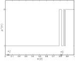
(a) Optimal global decision policy $\mu^{*}(\pi)$

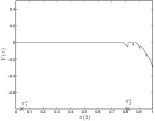
(b) Value function $V(\pi)$ for global decision policy

Figure 4: Optimal global decision policy for social learning based quickest time change detection for geometric distributed change time. The parameters are specified in Sec.IV-C. The optimal policy $\mu^{*}(\pi)\in\{1\text{ (announce change) },2\text{ (continue) }\}$ is characterized by a triple threshold – that is, it switches from 1 to 2 three times as the posterior $\pi(2)$ increases. The value function $V(\pi)$ is non-concave and discontinuous in $\pi$. As explained in the text, for $\pi(2)\in[0,\pi_{1}^{*}]$, all agents herd, while for $\pi(2)\in[\pi_{2}^{*},1]$ individual agents herd (see definitions in Sec.II-C).

V Coordination of Decisions in Sensing - Non-cooperative Game Approach

The discussion so far has dealt with Bayesian social learning models for sensing. In this section, we present a highly stylized non-Bayesian non-cooperative game theoretic learning approach for adaptive decision making amongst agents.

Social and economic situations often involve interacting decision making with diverging interests. Decision makers may act independently or form collaborative groups wherein enforceable binding agreements ensure coordination of joint decisions. For instance, a person may choose the same cellphone carrier as the majority of family and friends to take advantage of the free talk times. Social networks diffuse information and hence facilitate coordination of such cooperative/self-interested units. This section examines how global coordination of decisions can be obtained when self interested agents form a social network.

As mentioned in the Introduction, human-based sensing systems are comprised of agents with partial information and it is the dynamic interactions between agents that is of interest. This motivates the need for game theoretic learning models for agents interacting in social networks. Learning dynamics in games typically can be classified into Bayesian learning, adaptive learning and evolutionary dynamics. We have already focussed on Bayesian social learning in previous sections of the paper, and some further remarks are made in Sec.VI on global Bayesian games.

In this section we focus on adaptive learning where individual agents deploy simple rule-of-thumb strategies. The aim is to determine if such simple individual behaviour can result in sophisticated global behaviour. We are interested in cases where the global behaviour converges to the set of correlated equilibria.

V-A Correlated Equilibria and Related Work

The set of correlated equilibria is a more natural construct in decentralized adaptive learning environments than the set of Nash equilibria, since it allows for individual players to coordinate their actions. This coordination can lead to higher performance [34] than if each player chooses actions independently as required by a Nash equilibrium. As described in [75], it is unreasonable to expect in a learning environment that players act independently (as required by a Nash equilibrium) since the common history observed by all players acts as a natural coordination device. The set of correlated equilibria is also structurally simpler than the set of Nash equilibria; the set of correlated equilibria is a convex polytope in the set of randomized strategies whereas Nash equilibria are isolated points at the extrema of this set. Indeed, a feasible point in (25) is obtained straightforwardly by a linear programming solver.

Related works

A comprehensive textbook in game theoretic learning is [77]. Algorithms for game-theoretic learning are broadly classified into best response, fictitious play and regret matching. In general it is impossible to guarantee convergence to a Nash equilibrium without imposing conditions on the structure of the utility functions in the game. For supermodular games [78], best response algorithms can be designed to converge either to the smallest or largest Nash equilibrium. Fictitious play is one of the oldest and best known models of learning in games; we refer the reader to [79] for convergence of stochastic fictitious play algorithms. In this section we focus on regret-matching algorithms. Regret-matching as a strategy of play in long-run interactions has been introduced in [75, 76]. In [75], it is proved that when all agents share stage actions and follow the proposed regret-based adaptive procedure, the collective behavior converges to the set of correlated equilibria. In [76], the authors assumed that agents do not observe others’ actions and proposed a reinforcement learning procedure that converges to the set of correlated equilibria. More recently, [80, 81, 37, 38] consider learning in a dynamic setting where a regret matching type algorithm tracks a time varying set of correlated equilibria.

V-B Regret-Based Decision Making

Consider a non-cooperative repeated game comprising of $L$ agents. Each agent $l$ has a utility function $U^{l}(a^{1},\ldots,a^{L})$. Here $a^{l}$ denotes the action chosen by agent $l$ and $a^{-l}$ denote the actions chosen by all agents excluding agent $l$. The utility function can be quite general. For example, [82] considers the case in which the $L$ agents are organized into $M$ non-overlapping social (friendship) groups such that agents in a social group share the same utility function. It could also reflect reputation or privacy using the models in [49, 50].

Suppose each agent $l$ chooses its actions according to the following adaptive algorithm running over time $k=1,2,\ldots$:

1. At time $k+1$, choose action $a_{k+1}^{l}$ from probability mass function $\psi_{k+1}^{l}$, where

   $$\psi^{l}_{k+1}\left(i\right)=P\left(a_{k+1}^{l}=i|a_{k}^{l}\right)\\ =\left\{\begin{array}[]{ll}\frac{\left|r^{l}_{k}\left(i,j\right)\right|^{+}}{C},&j\neq a_{k}^{l}\\ 1-\sum_{j\neq i}\frac{\left|r^{l}_{k}\left(i,j\right)\right|^{+}}{C},&j=a_{k}^{l}.\\ \end{array}\right.$$ (22)

   Here $C$ is a sufficiently large positive constant so that $\psi^{l}_{k+1}$ is a valid probability mass function.

2. The regret matrix $r_{k}^{l}$ that determines the pmf $\psi^{l}_{k+1}$ is updated via the stochastic approximation algorithm

   $$r^{l}_{k}\left(i,j\right)=r^{l}_{k-1}\left(i,j\right)+\frac{1}{k}\Big{(}\bigl{[}U^{l}\left(j,{a}_{k}^{-l}\right)\\ -U^{l}\left(a_{k}^{l},{a}_{k}^{-l}\right)\bigr{]}I_{\{a_{k}^{l}=i\}}-r^{l}_{k-1}\left(i,j\right)\Big{)}.$$ (23)

Step 1 corresponds to each agent choosing its action randomly from a Markov chain with transition probability $\psi^{l}_{k+1}$. These transition probabilities are computed in Step 2 in terms of the regret matrix $r^{l}_{k}$ which is the time-averaged regret agent $l$ experiences for choosing action $i$ instead of action $j$ for each possible action $j\neq i$ (i.e., how much better off it would be if it had chosen action $j$ instead of $i$):

$$r^{l}_{n}\left(i,j\right)=\frac{1}{n}\sum_{k=1}^{n}\left[U^{l}\left(j,{a}_{k}^{-l}\right)-U^{l}\left(a_{k}^{l},{a}_{k}^{-l}\right)\right]\cdot I_{\{a_{k}^{l}=i\}}.$$ (24)

The above algorithm can be generalized to consider multiple social groups. If agents within each social group share their actions and have a common utility, then they can fuse their individual regrets into a regret for the social group. As shown in [82], this fusion of regrets can be achieved via a linear combination of the individual regrets where the weights of the linear combination depend on the reputation of the agents that constitute the social group.

V-C Coordination in Sensing

We now address the following question:

If each agent chooses its action according to the above regret-based algorithm, what can one say about the emergent global behavior?

By emergent global behavior, we mean the empirical frequency of actions taken over time by all agents. For each $L$-tuple of actions $(a^{l},a^{-l})$ define the empirical frequency of actions taken up to time $n$ as

$$z_{n}(a^{l},a^{-l})=\frac{1}{n}\sum_{k=1}^{n}I(a_{k}=a^{l},a_{k}^{-l}=a^{-l}).$$

The seminal papers [75] and [42] show that the empirical frequency of actions $z_{n}$ converges as $n\rightarrow\infty$ to the set of correlated equilibria of a non-cooperative game. Correlated equilibria constitute a generalization of Nash equilibria and were introduced by Aumann [34]. The set of correlated equilibria $\mathcal{C}_{e}$ is the set of probability distributions on the joint action profile $(a^{l},a^{-l})$ that satisfy

$$\mathcal{C}_{e}=\biggl{\{}\mu:\sum_{a^{-l}}\mu^{l}(j,a^{-l})[U^{l}((i,a^{-l}))-U^{l}((j,a^{-l}))]\\ \leq 0,\quad\forall l,j,i\biggr{\}}.$$ (25)

Here $\mu^{l}(j,a^{-l})=P^{l}(a^{l}=j,a^{-l})$ denotes the randomized strategy (joint probability) of player $l$ choosing action $j$ and the rest of the players choosing action $a^{-l}$. The correlated equilibrium condition (25) states that instead of taking action $j$ (which is prescribed by the equilibrium strategy $\mu^{l}(j,a^{-l})$), if player $l$ cheats and takes action $i$, it is worse off. So there is no unilateral incentive for any player to cheat.

To summarize, the above algorithm ensures that all agents eventually achieve coordination (consensus) in decision making – the randomized strategies of all agents converge to a common convex polytope $\mathcal{C}_{e}$. Step 2 of the algorithm requires that each agent knows its own utility and the actions of other agents – but agents do not need to know the utility functions of other agents. In [76] a ‘blind’ version of this regret-based algorithm is presented in which agents do not need to know the actions of other agents. These algorithms can be viewed as examples in which simple heuristic behavior by individual agents (choosing actions according to the measured regret) resulting in sophisticated global outcomes [42], namely convergence to $\mathcal{C}_{e}$ thereby coordinating decisions.

We refer to [37, 38, 80] for generalizations of the above algorithm to the tracking case where the step size for the regret matrix update is a constant. Such algorithms can track the correlated equilibria of games with time-varying parameters. Moreover [81] gives sufficient conditions for algorithm to converge to the set of correlated equilibria when the regrets from agents to other agents diffuse over a social network.

VI Closing Remarks

In this paper we have used social learning as a model for interactive sensing with social sensors. We summarize here some extensions of the social learning framework that are relevant to interactive sensing.

VI-1 Wisdom of Crowds

Surowiecki’s book [83] is an excellent popular piece that explains the wisdom-of-crowds hypothesis. The wisdom-of-crowds hypothesis predicts that the independent judgments of a crowd of individuals (as measured by any form of central tendency) will be relatively accurate, even when most of the individuals in the crowd are ignorant and error prone. The book also studies situations (such as rational bubbles) in which crowds are not wiser than individuals. Collect enough people on a street corner staring at the sky, and everyone who walks past will look up. Such herding behavior is typical in social learning.

VI-2 In which order should agents act?

In the social learning protocol, we assumed that the agents act sequentially in a pre-defined order. However, in many social networking applications, it is important to optimize the order in which agents act. For example, consider an online review site where individual reviewers with different reputations make their reviews publicly available. If a reviewer with high reputation publishes its review first, this review will unduly affect the decision of a reviewer with lower reputation. In other words, if the most senior agent “speaks” first it would unduly affect the decisions of more junior agents. This could lead to an increase in bias of the underlying state estimate. On the other hand, if the most junior agent is polled first, then since its variance is large, several agents would need to be polled in order to reduce the variance. We refer the reader to [85] for an interesting description of who should speak first in a public debate. It turns out that for two agents, the seniority rule is always optimal for any prior – that is, the senior agent speaks first followed by the junior agent; see [85] for the proof. However, for more than two agents, the optimal order depends on the prior, and the observations in general.

VI-3 Global Games for Coordinating Sensing

In the classical Bayesian social learning model of Sec.II, agents act sequentially in time. The global games model that has been studied in economics during the last two decades, considers multiple agents that act simultaneously by predicting the behavior of other agents. The theory of global games was first introduced in [86] as a tool for refining equilibria in economic game theory; see [87] for an excellent exposition. Global games are an ideal method for decentralized coordination amongst agents; they have been used to model speculative currency attacks and regime change in social systems, see [87, 88, 89].

The most widely studied form of a global game is a one-shot Bayesian game which proceeds as follows: Consider a continuum of agents in which each agent $i$ obtains noisy measurements $y^{i}$ of an underlying state of nature $x$. Assume all agents have the same observation likelihood density $p(y|x)$ but the individual measurements obtained by agents are statistically independent of those obtained by other agents. Based on its observation $y^{i}$, each agent takes an action $a^{i}\in\{1,2\}$ to optimize its expected utility $\mathbf{E}\{U(a^{i},\alpha)|y^{i}\})$ where $\alpha\in[0,1]$ denotes the fraction of all agents that take action 2. Typically, the utility $U(1,\alpha)$ is set to zero.

For example, suppose $x$ (state of nature) denotes the quality of a social group and $y^{i}$ denotes the measurement of this quality by agent $i$. The action $a^{i}=1$ means that agent $i$ decides not to join the social group, while $a^{i}=2$ means that agent $i$ joins the group. The utility function $U(a^{i}=2,\alpha)$ for joining the social group depends on $\alpha$, where $\alpha$ is the fraction of people that decide to join the group. In [88], the utility function is chosen as follows: If $\alpha\approx 1$, i.e., too many people join the group, then the utility to each agent is small since the group is too congested and agents do not receive sufficient individual service. On the other hand, if $\alpha\approx 0$, i.e., too few people join the group, then the utility is also small since there is not enough social interaction.

Since each agent is rational, it uses its observation $y^{i}$ to predict $\alpha$, i.e., the fraction of other agents that choose action 2. The main question is: What is the optimal strategy for each agent $i$ to maximize its expected utility?

It has been shown that for a variety of measurement noise models (observation likelihoods $p(y|x)$) and utility functions $U$, the symmetric Bayesian Nash equilibrium of the global game is unique and has a threshold structure in the observation. This means that given its observation $y^{i}$, it is optimal for each agent $i$ to choose its actions as follows:

$$a^{i}=\begin{cases}1&y^{i}<y^{*}\\ 2&y^{i}\geq y^{*}\end{cases}$$ (26)

where the threshold $y^{*}$ depends on the prior, noise distribution and utility function.

In the above example of joining a social group, the above result means that if agent $i$ receives a measurement $y^{i}$ of the quality of the group, and $y^{i}$ exceeds a threshold $y^{*}$, then it should join. This is yet another example of simple local behavior (act according to a threshold strategy) resulting in global sophisticated behavior (Bayesian Nash equilibrium). As can be seen, global games provide a decentralized way of achieving coordination amongst social sensors. In [89], the above one-shot Bayesian game is generalized to a dynamic (multi-stage) game operating over a possibly infinite horizon. Such games facilitate modelling the dynamics of how people join, interact and leave social groups.

The papers [39, 90] use global games to model networks of sensors and cognitive radios. In [88] it has been shown that the above threshold structure (26) for the Bayesian Nash equilibrium, breaks down if the utility function $U(2,\alpha)$ decreases too rapidly due to congestion. The equilibrium structure becomes much more complex and can be described by the following quotation [88]:

Nobody goes there anymore. It’s too crowded – Yogi Berra

VII Summary

This paper has considered social learning models for interaction among sensors where agents use their private observations along with actions of other agents to estimate an underlying state of nature. We have considered extensions of the basic social learning paradigm to online reputation systems in which agents communicate over a social network. Despite the apparent simplicity in these information flows, the systems exhibit unusual behavior such as herding and data incest. Also an example of social-learning for change detection was considered. Finally, we have discussed a non-Bayesian formulation, where agents seek to achieve coordination in decision making by optimizing their own utility functions - this was formulated as a game theoretic learning model.

The motivation for this paper stems from understanding how individuals interact in a social network and how simple local behavior can result in complex global behavior. The underlying tools used in this paper are widely used by the electrical engineering research community in the areas of signal processing, control, information theory and network communications.

Vikram Krishnamurthy [F] (vikramk@ece.ubc.ca) is a professor and Canada Research Chair at the Department of Electrical Engineering, University of British Columbia, Vancouver, Canada. Dr Krishnamurthy’s current research interests include statistical signal processing, computational game theory and stochastic control in social networks. He served as distinguished lecturer for the IEEE Signal Processing Society and Editor in Chief of IEEE Journal Selected Topics in Signal Processing. He received an honorary doctorate from KTH (Royal Institute of Technology), Sweden in 2013.

H. Vincent Poor [F] (poor@princeton.edu) is Dean of Engineering and Applied Science at Princeton University, where he is also the Michael Henry Strater University Professor. His interests include statistical signal processing and information theory, with applications in several fields. He is a member of the National Academy of Engineering, the National Academy of Sciences, and the Royal Academy of Engineering (UK). Recent recognition includes the 2010 IET Fleming Medal, the 2011 IEEE Sumner Award, the 2011 Society Award of IEEE SPS, and honorary doctorates from Aalborg University, the Hong Kong University of Science and Technology, and the University of Edinburgh.

References

- [1] N. Eagle and A. Pentland, “Reality mining: Sensing complex social systems,” Personal and Ubiquitous Computing, vol. 10, no. 4, pp. 255–268, 2006.
- [2] C. Aggarwal and T. Abdelzaher, “Integrating sensors and social networks,” Social Network Data Analytics, pp. 397–412, 2011.
- [3] A. Campbell, S. E. B, N. Lane, E. Miluzzo, R. Peterson, H. Lu, X. Hong, X. Zheng, M. Musolesi, K. Fodor, and G. Ahn, “The rise of people-centric sensing,” IEEE Internet Computing, vol. 12, no. 4, pp. 12–21, 2008.
- [4] J. Burke, D. Estrin, M. Hansen, A. Parker, N. Ramanathan, S. Reddy, and M. Srivastava, “Participatory sensing,” in World Sensor Web Workshop, ACM Sensys, Boulder, 2006.
- [5] A. Rosi, M. Mamei, F. Zambonelli, S. Dobson, G. Stevenson, and J. Ye, “Social sensors and pervasive services: Approaches and perspectives,” in 2011 IEEE International Conference on Pervasive Computing and Communications Workshops (PERCOM Workshops),. IEEE, 2011, pp. 525–530.
- [6] R. Lee and K. Sumiya, “Measuring geographical regularities of crowd behaviors for twitter-based geo-social event detection,” in Proceedings of the 2nd ACM SIGSPATIAL International Workshop on Location Based Social Networks. ACM, 2010, pp. 1–10.
- [7] Z. Cheng, J. Caverlee, and K. Lee, “You are where you tweet: a content-based approach to geo-locating twitter users,” in Proceedings of the 19th ACM international conference on Information and knowledge management. ACM, 2010, pp. 759–768.
- [8] M. Trusov, A. V. Bodapati, and R. E. Bucklin, “Determining influentual users in internet social networks,” Journal of Marketing Research, vol. XLVII, pp. 643–658, Aug. 2010.
- [9] T. Sakaki, M. Okazaki, and Y. Matsuo, “Earthquake shakes twitter users: real-time event detection by social sensors,” in Proceedings of the 19th international conference on World wide web. New York, NY, USA: ACM, 2010, pp. 851–860.
- [10] J. Bollen, H. Mao, and X. Zeng, “Twitter mood predicts the stock market,” Journal of Computational Science, vol. 2, no. 1, pp. 1–8, 2011.
- [11] B. Pang and L. Lee, “Opinion mining and sentiment analysis,” Foundations and trends in information retrieval, vol. 2, no. 1-2, pp. 1–135, 2008.
- [12] S. Asur and B. A. Huberman, “Predicting the future with social media,” in 2010 IEEE/WIC/ACM International Conference on Web Intelligence and Intelligent Agent Technology (WI-IAT), vol. 1. IEEE, 2010, pp. 492–499.
- [13] B. Ifrach, C. Maglaras, and M. Scarsini, “Monopoly pricing in the presence of social learning,” NET Institute Working Paper No. 12-01, 2011.
- [14] M. Luca, Reviews, reputation, and revenue: the case of Yelp.com, Technical Report 12-016. Harvard Business School, 2011.
- [15] A. Banerjee, “A simple model of herd behavior,” Quaterly Journal of Economics, vol. 107, no. 3, pp. 797–817, August 1992.
- [16] S. Bikchandani, D. Hirshleifer, and I. Welch, “A theory of fads, fashion, custom, and cultural change as information cascades,” Journal of Political Economy, vol. 100, no. 5, pp. 992–1026, October 1992.
- [17] C. Chamley, Rational herds: Economic Models of Social Learning. Cambridge University Press, 2004.
- [18] D. Acemoglu and A. Ozdaglar, “Opinion dynamics and learning in social networks,” Dynamic Games and Applications, vol. 1, no. 1, pp. 3–49, 2011.
- [19] I. Lobel, D. Acemoglu, M. Dahleh, and A. Ozdaglar, “Preliminary results on social learning with partial observations,” in Proceedings of the 2nd International Conference on Performance Evaluation Methodolgies and Tools. Nantes, France: ACM, 2007.
- [20] D. Acemoglu, M. Dahleh, I. Lobel, and A. Ozdaglar, “Bayesian learning in social networks,” National Bureau of Economic Research, Working Paper 14040, May 2008.
- [21] T. Cover and M. Hellman, “The two-armed-bandit problem with time-invariant finite memory,” IEEE Trans. Information Theory, vol. 16, no. 2, pp. 185–195, 1970.
- [22] M. Hellman and T. Cover, “Learning with finite memory,” The Annals of Mathematical Statistics, vol. 41, no. 3, pp. 765–782, 1970.
- [23] C. Chamley, A. Scaglione, and L. Li, “Models for the diffusion of beliefs in social networks: An overview,” IEEE Signal Processing Magazine, vol. 30, no. 3, pp. 16–29, 2013.
- [24] V. Krishnamurthy and H. V. Poor, “Social learning and Bayesian games in multiagent signal processing: How do local and global decision makers interact?” IEEE Signal Processing Magazine, vol. 30, no. 3, pp. 43–57, 2013.
- [25] M. Avellaneda and S. Stoikov, “High-frequency trading in a limit order book,” Quantitative Finance, vol. 8, no. 3, pp. 217–224, Apr 2008.
- [26] D. López-Pintado, “Contagion and coordination in random networks,” International Journal of Game Theory, vol. 34, no. 3, pp. 371–381, 2006.
- [27] ——, “Diffusion in complex social networks,” Games and Economic Behavior, vol. 62, no. 2, pp. 573–590, 2008.
- [28] M. Granovetter, “Threshold models of collective behavior,” American journal of sociology, pp. 1420–1443, 1978.
- [29] J. Goldenberg, B. Libai, and E. Muller, “Talk of the network: A complex systems look at the underlying process of word-of-mouth,” Marketing letters, vol. 12, no. 3, pp. 211–223, 2001.
- [30] E. Mossel and S. Roch, “On the submodularity of influence in social networks,” in Proceedings of 39th Annual ACM symposium on Theory of Computing. ACM, 2007, pp. 128–134.
- [31] N. Chen, “On the approximability of influence in social networks,” SIAM Journal on Discrete Mathematics, vol. 23, no. 3, pp. 1400–1415, 2009.
- [32] S. Bharathi, D. Kempe, and M. Salek, “Competitive influence maximization in social networks,” in Internet and Network Economics. Springer, 2007, pp. 306–311.
- [33] K. Apt and E. Markakis, “Diffusion in social networks with competing products,” in Algorithmic Game Theory. Springer, 2011, pp. 212–223.
- [34] R. J. Aumann, “Correlated equilibrium as an expression of bayesian rationality,” Econometrica, vol. 55, no. 1, pp. 1–18, 1987.
- [35] F. Vega-Redondo, Complex Social Networks. Cambridge University Press, 2007, vol. 44.
- [36] M. Jackson, Social and economic networks. Princeton University Press, 2010.
- [37] V. Krishnamurthy, M. Maskery, and G. Yin, “Decentralized activation in a ZigBee-enabled unattended ground sensor network: A correlated equilibrium game theoretic analysis,” IEEE Trans. Signal Proc., vol. 56, no. 12, pp. 6086–6101, December 2008.
- [38] M. Maskery, V. Krishnamurthy, and Q. Zhao, “Decentralized dynamic spectrum access for cognitive radios: Cooperative design of a non-cooperative game,” IEEE Trans. Commun., vol. 57, no. 2, pp. 459–469, 2008.
- [39] V. Krishnamurthy, “Decentralalized activation in dense sensor networks via global games,” IEEE Trans. Signal Proc., vol. 56, no. 10, pp. 4936–4950, 2008.
- [40] ——, “Bayesian sequential detection with phase-distributed change time and nonlinear penalty – a lattice programming POMDP approach,” IEEE Trans. Information Theory, vol. 57, no. 3, pp. 7096–7124, Oct. 2011.
- [41] ——, “Quickest detection POMDPs with social learning: Interaction of local and global decision makers,” IEEE Trans. Information Theory, vol. 58, no. 8, pp. 5563–5587, 2012.
- [42] S. Hart, “Adaptive heuristics,” Econometrica, vol. 73, no. 5, pp. 1401–1430, 2005.
- [43] J. Predd, S. R. Kulkarni, and H. V. Poor, “A collaborative training algorithm for distributed learning,” IEEE Trans. Information Theory, vol. 55, no. 4, pp. 1856–1871, 2009.
- [44] G. Wang, S. R. Kulkarni, H. V. Poor, and D. Osherson, “Aggregating large sets of probabilistic forecasts by weighted coherent adjustment,” Decision Analysis, vol. 8, no. 2, pp. 128–144, June 2011.
- [45] G. Ellison and D. Fudenberg, “Rules of thumb for social learning,” Journal of Political Economy, vol. 101, no. 4, pp. pp. 612–643, 1993.
- [46] ——, “Word-of-mouth communication and social learning,” The Quarterly Journal of Economics, vol. 110, no. 1, pp. 93–125, 1995.
- [47] L. Smith and P. Sorensen, “Informational herding and optimal experimentation,” Economics Group, Nuffield College, University of Oxford, Economics Papers 139, 1997. [Online]. Available: http://ideas.repec.org/p/nuf/econwp/139.html
- [48] Y. Ephraim and N. Merhav, “Hidden Markov processes,” IEEE Trans. Information Theory, vol. 48, pp. 1518–1569, June 2002.
- [49] L. Mui, “Computational models of trust and reputation: Agents, evolutionary games, and social networks,” Ph.D. dissertation, MIT, Department of Electrical Enginering and Computer Science, 2002.
- [50] E. Gudes, N. Gal-Oz, and A. Grubshtein, “Methods for computing trust and reputation while preserving privacy,” in Data and Applications Security XXIII. Springer, 2009, pp. 291–298.
- [51] A. R. Cassandra, “Exact and approximate algorithms for partially observed markov decision process,” Ph.D. dissertation, Brown University, 1998.
- [52] W. Lovejoy, “Some monotonicity results for partially observed Markov decision processes,” Operations Research, vol. 35, no. 5, pp. 736–743, Sept.-Oct. 1987.
- [53] U. Rieder, “Structural results for partially observed control models,” Methods and Models of Operations Research, vol. 35, no. 6, pp. 473–490, 1991.
- [54] V. Krishnamurthy and D. Djonin, “Structured threshold policies for dynamic sensor scheduling–a partially observed Markov decision process approach,” IEEE Trans. Signal Proc., vol. 55, no. 10, pp. 4938–4957, Oct. 2007.
- [55] V. Krishnamurthy, “How to schedule measurements of a noisy Markov chain in decision making?” IEEE Trans. Information Theory, vol. 59, no. 9, July 2013.
- [56] W. Lovejoy, “On the convexity of policy regions in partially observed systems,” Operations Research, vol. 35, no. 4, pp. 619–621, July-August 1987.
- [57] V. Krishnamurthy and M. Hamdi, “Mis-information removal in social networks: Dynamic constrained estimation on directed acyclic graphs,” IEEE Journal Selected Topics in Signal Processing, vol. 7, no. 2, pp. 333–346, May 2013.
- [58] B. Tuttle, “Fact-checking the crowds: How to get the most out of hotel-review sites,” Time magazine, July 2013.
- [59] G. Adomavicius and A. Tuzhilin, “Toward the next generation of recommender systems: A survey of the state-of-the-art and possible extensions,” IEEE Transactions on Knowledge and Data Engineering, vol. 17, no. 6, pp. 734–749, 2005.
- [60] I. Konstas, V. Stathopoulos, and J. M. Jose, “On social networks and collaborative recommendation,” in Proceedings of the 32nd international ACM SIGIR conference on Research and development in information retrieval. ACM, 2009, pp. 195–202.
- [61] Y. Kanoria and O. Tamuz, “Tractable Bayesian social learning on trees,” in Proceedings IEEE International Symposium on Information Theory (ISIT), Jul. 2012, pp. 2721 –2725.
- [62] T. Brehard and V. Krishnamurthy, “Optimal data incest removal in Bayesian decentralized estimation over a sensor network,” in IEEE International Conference on Acoustics Speech and Signal Processing ICASSP (2007), 2007, pp. 173–176.
- [63] J. Pearl, “Fusion, propagation, and structuring in belief networks,” Artificial Intelligence, vol. 29, no. 3, pp. 241 – 288, 1986.
- [64] K. Murphy, Y. Weiss, and M. Jordan, “Loopy belief propagation for approximate inference: an empirical study,” in Proceedings of Fifteenth Conference Uncertainty in Artificial Intelligence, 1999, pp. 467–475.
- [65] J. Yedidia, W. Freeman, and Y. Weiss, “Constructing free-energy approximations and generalized belief propagation algorithms,” IEEE Trans. Information Theory, vol. 51, no. 7, pp. 2282–2312, 2005.
- [66] R. J. Aumann, “Agreeing to disagree,” The Annals of Statistics, Nov. 1976.
- [67] J. Geanakoplos and H. Polemarchakis, “We can’t disagree forever,” Journal of Economic Theory, vol. 28, no. 1, pp. 192 – 200, 1982.
- [68] V. Borkar and P. Varaiya, “Asymptotic agreement in distributed estimation,” IEEE Trans. Auto. Control, vol. 27, no. 3, pp. 650–655, 1982.
- [69] R. Bond, C. Fariss, J. Jones, A. Kramer, C. Marlow, J. Settle, and J. Fowler, “A 61-million-person experiment in social influence and political mobilization,” Nature, vol. 489, pp. 295–298, September 2012.
- [70] M. Hamdi and V. Krishnamurthy, “Removal of Data Incest in Multi-agent Social Learning in Social Networks,” ArXiv e-prints, Sep. 2013.
- [71] M. Benaïm and J. Weibull, “Deterministic approximation of stochastic evolution in games,” Econometrica, vol. 71, no. 3, pp. 873–903, 2003.
- [72] V. Krishnamurthy and A. Aryan, “Quickest detection of market shocks in agent based models of the order book,” in Proceedings 51st IEEE Conference on Decision and Control, Maui, Hawaii, Dec. 2012.
- [73] H. V. Poor and O. Hadjiliadis, Quickest Detection. Cambridge University Press, 2008.
- [74] A. Shiryaev, “On optimum methods in quickest detection problems,” Theory of Probability and its Applications, vol. 8, no. 1, pp. 22–46, 1963.
- [75] S. Hart and A. Mas-Colell, “A simple adaptive procedure leading to correlated equilibrium,” Econometrica, vol. 68, no. 5, pp. 1127–1150, 2000.
- [76] ——, “A reinforcement procedure leading to correlated equilibrium,” in Economic Essays: A Festschrift for Werner Hildenbrand, G. Debreu, W. Neuefeind, and W. Trockel, Eds. Springer, 2001, pp. 181–200.
- [77] D. Fudenberg and D. Levine, The Theory of Learning in Games. MIT Press, 1999.
- [78] D. Topkis, Supermodularity and Complementarity. Princeton University Press, 1998.
- [79] J. Hofbauer and W. Sandholm, “On the global convergence of stochastic fictitious play,” Econometrica, vol. 70, no. 6, pp. 2265–2294, Nov. 2002.
- [80] O. Namvar, V. Krishnamurthy, and G. Yin, “Distributed tracking of correlated equilibria in regime switching noncooperative games,” IEEE Trans. Auto. Control, vol. 58, no. 10, pp. 2435–2450, 2013.
- [81] ——, “Distributed energy-aware diffusion least mean squares: Game-theoretic learning,” IEEE Journal of Selected Topics in Signal Processing, vol. 7, no. 5, p. 821, 2013.
- [82] ——, “Diffusion based collaborative decision making in noncooperative social network games,” in Proceedings First Global Conference on Signal and Information Processing, Austin, Dec. 2013.
- [83] J. Surowiecki, The Wisdom of Crowds. Anchor, 2005.
- [84] C. Anderson and G. J. Kilduff, “Why do dominant personalities attain influence in face-to-face groups? the competence-signaling effects of trait dominance,” Journal of Personality and Social Psychology, vol. 96, no. 2, pp. 491–503, 2009.
- [85] M. Ottaviani and P. Sørensen, “Information aggregation in debate: Who should speak first?” Journal of Public Economics, vol. 81, no. 3, pp. 393–421, 2001.
- [86] H. Carlsson and E. van Damme, “Global games and equilibrium selection,” Econometrica, vol. 61, no. 5, pp. 989–1018, Sept. 1993.
- [87] S. Morris and H. Shin, “Global games: Theory and applications,” in Advances in Economic Theory and Econometrics: Proceedings of Eight World Congress of the Econometric Society. Cambridge University Press, 2000.
- [88] L. Karp, I. Lee, and R. Mason, “A global game with strategic substitutes and complements,” Games and Economic Behavior, vol. 60, pp. 155–175, 2007.
- [89] G. Angeletos, C. Hellwig, and A. Pavan, “Dynamic global games of regime change: Learning, multiplicity, and the timing of attacks,” Econometrica, vol. 75, no. 3, pp. 711–756, 2007.
- [90] V. Krishnamurthy, “Decentralized spectrum access amongst cognitive radios-an interacting multivariate global game-theoretic approach,” IEEE Trans. Signal Proc., vol. 57, no. 10, pp. 3999–4013, Oct. 2009.