Configurations of a new atomic interferometer for gravitational wave detection

Abstract

Recently, the configuration using atomic interferometers (AIs) had been suggested for the detection of gravitational waves. A new AI with some additional laser pulses for implementing large momentum transfer was also put forward, in order to improve the influence of shot noise and laser frequency noise. In the paper, we use the sensitivity function to analyze all possible configurations of the new AI and to distinguish how many momenta are transferred in a specific configuration. With the analysis for the new configuration, we explore the detection scheme of gravitational wave further, in particular, for the amelioration of the laser frequency noise. We find that the amelioration is definite in such scheme, but novelly, in some cases the frequency noise can be canceled completely by using a proper data processing method.

I Introduction

Since gravitational waves were predicted from the theory of General Relativity, a direct detection of gravitational waves had become an exciting frontier of experimental physics gvlb13 . The initial detection scheme was related to the resonant bar detectors jw69 which would be mechanically disturbed by passing gravitational waves, and then some other detectors which had one or more arms with its arm length influenced by passing gravitational waves were put forward. For the latter, the VIRGO aaa10 and LIGO aaa09 are the most sensitive detectors of this class as an kind of interferometer modulated by the change of the apparent distance between mirrors by passing gravitational waves. Many efforts had also been made to improve the frequency range and the sensitivity of the possible probed gravitational waves, e.g. Advanced LIGO gmh10 , and a large space-based laser interferometer gravitational wave detector, LISA ep96 . Although there is no any definite and direct evidence to show the existence of gravitational waves up to now, these efforts gave an upper limit on the stochastic gravitational-wave background of cosmological origin lv09 which was considered as a realistic observable tied directly to the quantization of gravity in a recent paper kw13 .

Another direction of efforts to detect gravitational waves is related to the use of atomic coherence. The first scheme along this direction is MIGO (Matter-wave Interferometric Gravitational-wave Observatory) cs04 ; sc04 in which the atom wave is used with the same role as the photons in LIGO. In particular, it was shown rbp06 recently that the scheme based on MIGO would no better than LIGO, which made the attention focused on the MIGO reduced to some extent. However, the appearance of MIGO stimulated the thoughts on using atomic interferometers to detect gravitational waves. An interesting design along the line is AGIS (Atomic Gravitational Wave Interferometric Sensor) dgr08 which works with a similar mechanism to LIGO but replacing the macroscopic mirrors with freely falling atoms. The use of freely falling atoms or atomic interferometers as local inertial sensors reduced the requirement of elaborate seismic isolation which limits the sensitivity of LIGO at Hz-band or lower frequencies, so the AGIS have an advantage over LIGO by detecting gravitational waves between 0.01 and 100 Hz. However, in AGIS, the Raman process in the atomic interferometers still induces an uncontrollable noise through the laser phase fluctuations which is also a dominant noise background for the detection of gravitational waves using LIGO. The reason of existence of laser frequency noises in AGIS dghk08 is the use of two laser beams in the interaction with the atoms, in which the pulses from the control laser are common to both interferometers and the phase contributions from this laser would be canceled in the final differential phase shift, but the noise in the phase of the passive laser cannot be canceled completely. This leads to a recent suggestion yt10 for the gravitational wave detection using the similar structure to AGIS but replacing the local inertial sensors with single-laser atom interferometers, which overcomes the laser frequency noise existed in the gravitational wave detection using LIGO but still inherits the advantages of AGIS to the suppression of vibration noise.

However, the measurement of interferometry is also limited by the shot noise which is related to the number of particles attending the interference process. Thus following the optimistic assumption dgr08 about the number of atom when operating an atomic interferometer, the shot noise is still larger in an atomic interferometer than in an optical interferometer. In particular, the typical number of photon impinging on a photo detector is easily increased than the number of atoms in an atomic interferometer. Thus besides developing a new technology to increase the number of atoms, one has to use the large momentum transfer (LMT) dgr08 ; mclh08 to compensate for the low number of atoms. Based on this background, a new method for gravitational wave detection with atomic sensors was recently suggested ghkr13 , which not only overcame the laser frequency noise using single-laser atomic interferometers, but also realized the LMT by adding some laser pulses between the basic beam splitter and mirror pulses. However, in Ref. ghkr13 , the authors gave only a prototypical illumination for the mechanism realizing LMT, and didn’t make the detailed analysis for the possible configurations of the new interferometer. This forms the main purpose of this paper, that is to analyze the configurations of the new interferometer and the difference of the momentum transfer for different configurations. On the other hand, we will also attempt to analyze the cancellation of laser frequency noises with a direct and explicit mathematical expression.

In order to analyze the structure of new atomic interferometers, we introduce the sensitivity function ccl05 to distinguish the different momentum transfer for different structures and thus the complex calculation for the final total phase difference using the standard method of non-relativistic quantum mechanics can be avoided. The second section of the paper will give a brief introduction of sensitivity function, in particular for its application to sense the signal about the gravitational field. In the third section, we analyze the possible configurations for the new interferometers and find some interesting phenomena for some configurations. In the fourth section, we present the results of laser frequency noise cancellation with an analysis of the total laser phase difference. In particular, we find the method of the time-delay interferometry (TDI) used in Ref. yt10 to cancel the laser frequency noise is not applicable to the scheme suggested in Ref. ghkr13 . Finally, we summarize our conclusions in the fifth section.

II Sensitivity function

In this section we will revisit the sensitivity function, without loss of generality, in the time-domain atomic interferometer proposed firstly by Kasevich and Chu kc91 . The interferometer consists of beam splitter-mirror-beam splitter ($\frac{\pi}{2}-\pi-\frac{\pi}{2}$) optical pulse sequence, and its sensitivity is limited to a large extent by the phase noise derived from the lasers as well as the residual vibrations. Similar to the Ref. ccl05 , our investigation for the sensitivity function here is under the assumption of short laser pulses with the description of pure plane waves.

In the interferometer we considered here, the output of the results is presented by the population change of atomic number, e.g. the probability of finding the atom remained in the ground state when leaving the interferometer is $P=\frac{1+\cos\left(\Delta\Phi\right)}{2}$ where $\Delta\Phi=\Delta\Phi_{s}+\Delta\Phi_{n}$ is the total phase difference dghk08 ; kc92 ; sc94 ; pcc97 ; zcz13 between the two paths of the interferometer, which is also the basis of experimental observation. In a local gravitational measurement around the Earth, the leading order of the signal can be calculated as $\Delta\Phi_{s}=kgT^{2}$ where $k$ is the effective laser-field wavevector, $T$ is the interrogation time between two sequent laser pulses, and $g$ is the local gravitational acceleration. And $\Delta\Phi_{n}=\phi_{1}-2\phi_{2}+\phi_{3}$ is the interferometric phase from the interaction between three laser pulses and atoms, and it is usually locked to the value $\frac{\pi}{2}$ such that the transition probability is $\frac{1}{2}$ which ensures the highest sensitivity to any interferometric phase fluctuations. From the perspective of the configuration, the signal can also be regarded as derived from a certain kind of interference, e.g. its influence is included in the interferometric phase $\Delta\Phi_{n}$. Thus it is not hard to understand why the noises usually constrain the sensitivity of the interferometer. In the following we will consider $\Delta\Phi=\Delta\Phi_{n}$ and $\Delta\Phi_{s}$ enters into the total phase difference as the influence of gravitational field on the interferometric phase. In particular, we will consider the same interferometer but with a single laser pulse to interact with the atom, and thus the Raman process is replaced with a single photon transition and the redundant effects related to the ac Stark shifts would disappear wyc94 ; pcc01 . In this case, the signal, expressed by the leading order phase shift in a local gravitational field, is proportional to the atomic energy level difference, which will be seen later.

As suggested firstly by Dick gjd87 and then investigated in detail by Cheinet, et al ccl05 , the sensitivity of a time-domain atomic interferometer can be characterized by the sensitivity function which quantifies the influence of a relative laser phase shift $\delta\phi$ occurring at a time $t$ during the interferometer sequence onto the transition probability $\delta P\left(\delta\phi,t\right)$; it is then defined in Ref. gjd87 as

$$g\left(t\right)=2\ast\underset{\delta\phi\rightarrow 0}{\lim}\frac{\delta P\left(\delta\phi,t\right)}{\delta\phi}.$$ (1)

If the time origin is chosen at the middle of the second Raman pulse, the sensitivity function $g\left(t\right)$ is an odd function. For the three pulses $\frac{\pi}{2}-\pi-\frac{\pi}{2}$ with durations respectively $\tau-2\tau-\tau$, we choose the initial time $t_{i}=-T$ and the final time $t_{f}=T$ to get the expression of the sensitivity function as

$$g(t)=\left\{\begin{array}[c]{c}\sin(\Omega(T+t))\ \ \ ,-T\leqslant t<-T+\tau\\ \ 1\ \ \ \ \ \ \ \ \ \ \ \ \ ,-T\ +\tau\leqslant t<-\tau\\ -\sin\Omega t\ \ \ \ \ \ \ \ ,-\tau\leqslant t<\tau\\ -1\ \ \ \ \ \ \ \ \ \ \ \ ,\tau\leqslant t<T-\tau\\ -\sin\Omega(T-t)\ \ \ \ ,T-\tau\leqslant t\leqslant T\end{array}\right.$$ (2)

where $\Omega$ is the effective Rabi frequency and $g(t)=0$ for $\left|t\right|>T$ due to the phase jump occurs outside the interferometer. As seen in Fig.1, the sensitivity function $g(t)$ is indeed an odd function, so in the analysis of the next section we will present a sensitivity function with the part only for $t<0$. Usually the Fourier transform of the sensitivity function is required, since the noises related closely to the analysis of the sensitivity of an interferometer can be expressed in terms of a power spectral density which is expanded with the frequency. Thus the transfer function which is introduced in the appendix1 is usually used in the analysis of the sensitivity, but in the present paper we focus on the analysis of the structure of the interferometer, so the sensitivity function is enough. We will also use the transfer function when we discuss the advantages of some kinds of interferometers, e.g. the transfer of the influence of the noises.

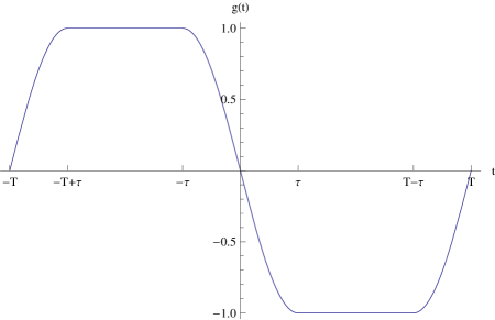
Figure 1: the sensitivity function g(t)

As shown in Ref. ccl05 , one can evaluate the fluctuations of the interferometric phase $\Delta\Phi$ caused by an arbitrary perturbation $\phi\left(t\right)$ by

$$\Delta\Phi=\int_{-\infty}^{+\infty}g\left(t\right)\frac{d\phi\left(t\right)}{dt}dt.$$ (3)

Of course, the influence due to the atomic acceleration will be sensed by the interferometer through the sensitivity function. In general, this type of time-domain atomic interferometer discussed here is an accelerometer. In the free evolution of the atom, its phase changes by $\phi_{g}\left(t\right)=\frac{\omega_{a}}{c}x=\frac{\omega_{a}}{c}(x_{0}+v_{0}t+\frac{1}{2}gt^{2})$ where $x_{0}$, $v_{0}$ are the initial position and velocity of the atom. Then using the Eq. (3), we recover the signal of the interferometer

$$\Delta\Phi_{s}=\frac{\omega_{a}}{c}gT^{2}+O(1)$$ (4)

where $\omega_{a}$ is the atomic energy level difference and $O(1)$ represents the terms related to $\tau$ or $\frac{1}{\Omega}$, which are tiny values compared to the leading term. If the relativistic calculation is considered as in Ref. dghk08 and the corresponding geodesic is used to get the phase disturbance $\phi_{g}\left(t\right)$, more effects will be presented. Here the calculation is feasible, because the phase change of the atom induced by the gravitational field during the free evolution is equivalent to the phase change of the laser pulse by the fact that the gravitational field changes the positions of the interaction between the laser pulses and atoms. On the other hand, in the free evolution, the phase changes actually are $\phi_{g0}\left(t\right)=\frac{\omega_{0}}{c}x$ where $\omega_{0}$ is the energy of atomic ground state and $\phi_{g1}\left(t\right)=\frac{\omega_{1}}{c}x$ where $\omega_{1}$ is the energy of atomic excited state, but after the first beam splitter, the state of atom is a superposition of the ground and excited states, so we only need to consider the change of the relative phase, $\phi_{g}\left(t\right)=\frac{\omega_{a}}{c}x$ where $\omega_{a}=\omega_{1}-\omega_{0}$.

III Configurational analysis of a new atomic interferometer

In this section, we will use the sensitivity function to analyze the configuration suggested in Ref. ghkr13 , which can be understood as a variant of a light-pulse de Broglie wave interferometer in Mach-Zender configuration. This kind of atomic interferometer is derived from the time-domain atomic interferometer introduced in the last section, but with an obvious difference by adding some pulses between the basic beam splitters and the mirror pulse which leads to a large momentum transfer (LMT). All added pulses are $\pi$ pulses (to distinguish the basic mirror $\pi$ pulse, we call these specific $\pi$ pulses) which are refined to interact only with the required halves of atoms, unlike the three basic pulses that interact with all atoms simultaneously but with different influences on each half. In order to realize the LMT, these specific $\pi$ pulses must be arranged carefully. Here we will show that for the given number of the specific $\pi$ pulses, the momentum transfer will be dependent on the sequence (that includes the consideration of the direction of pulses and which halves of atoms will interact with the laser pulses) and the time (that means what time each pulse is applied). The case of $N=3$ is used to show this. The sign $N$ is slightly different from that used in Ref. ghkr13 , and here our signs are related to the final leading order phase shift for the case with the largest momentum transfer, e.g. for the interferometer of $N=3$ presented in Fig.2, it is $\sim 3\omega_{a}gT^{2}/c$. In particular, the case presented in the FIG. 2 of Ref. ghkr13 is $N=2$ according to our rule of signs.

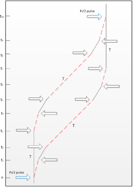
Figure 2: A spacetime disgram of the proposed N=3 configuration. The non-labelled arrows represent the $\pi$ pulses, and the directions of the arrows is along the motion of the pulses. The joint points linking the solid and dashed lines indicate the vertices at which the laser interacts with the atom.

It is seen easily from the interferometer of $N=3$ that there are four specific $\pi$ pulses before the basic mirror pulse and the arrangement presented in Fig.2 is the case with the largest momentum transfer. Actually, there are many other ways to arrange the four $\pi$ pulses, and the final leading order phase shifts will include the possible results $\sim$ $2\omega_{a}gT^{2}/c$, $\omega_{a}gT^{2}/c$ and $0$. There are $30$ possible structures in our consideration with different sequences and different times, but there is only one that can realize the largest momentum transfer, i.e. the case of the final leading order phase shift is $3\omega_{a}gT^{2}/c$. It is pointed out that the counting of all possible configurations of interferometers is based on the assumption that the laser emitter is fixed on a position or the basic beam splitters are from the same direction. Then there is a natural problem: how can we know which is LMT and how many momenta are transferred. One standard method is to calculate all of the interactions included in the process of the interferometer to get the final leading phase shift, e.g. using the method in Ref. dghk08 , but the relativistic calculation is not required. Here we will provide another interesting method with the sensitivity function. For the case of $N=3$ in Fig.2, due to the odd symmetry of the sensitivity function, we write it only for $t<0$,

$$g_{3}(t)=\left\{\begin{array}[c]{c}\sin\Omega(t+T)\ \ \ \ \ \ \ \ \ \ \ \ \ \ ,-T\leqslant t<-T+\tau\\ \ \ \ \ \ \ \ \ \ 1\ \ \ \ \ \ \ \ \ \ \ \ \ \ \ \ \ \ \ ,-T+\tau\leqslant t<-T+3\tau\\ \frac{1}{2}[3-\cos\Omega(T+t-3\tau)]\ \ \ \ \ \ ,-T+3\tau\leqslant t<-T+5\tau\\ \ \ \ \ \ \ \ \ \ \ 2\ \ \ \ \ \ \ \ \ \ \ \ \ \ \ \ \ \ \ ,-T+5\tau\leqslant t<-T+7\tau\\ \frac{1}{2}[5-\cos\Omega(T+t-7\tau)]\ \ \ \ \ \ ,-T+7\tau\leqslant t<-T+9\tau\\ \ \ \ \ \ \ 3\ \ \ \ \ \ \ \ \ \ \ \ \ \ \ \ \ \ \ ,-T+9\tau\leqslant t<-9\tau\\ \ \frac{1}{2}[5+\cos\Omega(t+9\tau)]\ \ \ \ \ \ \ \ \ \ ,-9\tau\leqslant t<-7\tau\\ \ \ 2\ \ \ \ \ \ \ \ \ \ \ \ \ \ \ \ \ \ \ ,-7\tau\leqslant t<-5\tau\\ \ \ \frac{1}{2}[3+\cos\Omega(t+5\tau)]\ \ \ \ \ \ \ \ \ \ ,-5\tau\leqslant t<-3\tau\\ \ 1\ \ \ \ \ \ \ \ \ \ \ \ \ \ \ \ \ \ \ ,-3\tau\leqslant t<-\tau\\ \ -\sin\Omega t\ \ \ \ \ \ \ \ \ \ \ \ \ \ \ \ ,-\tau\leqslant t<0\end{array}\right.$$

which is calculated detailedly in the appendix2. Then for the information from the gravitational field, the leading order leads to,

$$\Delta\Phi_{3}=\int_{-\infty}^{+\infty}g_{3}\left(t\right)\frac{d\phi_{g}\left(t\right)}{dt}dt=3\frac{\omega_{a}}{c}gT^{2},$$ (5)

and as expected, it includes the largest momentum transfer. This result is also seen implicitly from the sensitivity function itself, e.g. $g_{3}\left(t\right)=3$, for $-T+9\tau\leqslant t<-9\tau$, as presented in Fig.3. However, the time that the specific $\pi$ pulses are applied works definitely, e.g. the time for the eleven pulses calculated here is t1: $\left(-T\right)\rightarrow\left(-T+3\tau\right)\rightarrow\left(-T+7\tau\right)\rightarrow\left(-9\tau\right)\rightarrow\left(-5\tau\right)\rightarrow\left(-\tau\right)\rightarrow\left(3\tau\right)\rightarrow\left(7\tau\right)\rightarrow\left(T-9\tau\right)\rightarrow\left(T-5\tau\right)\rightarrow\left(T-\tau\right)$. If we change the times but don’t change the sequence, e.g. when the time take t2: $\left(-T\right)\rightarrow\left(-T+3\tau\right)\rightarrow\left(-13\tau\right)\rightarrow\left(-9\tau\right)\rightarrow\left(-5\tau\right)\rightarrow\left(-\tau\right)\rightarrow\left(3\tau\right)\rightarrow\left(7\tau\right)\rightarrow\left(9\tau\right)\rightarrow\left(T-5\tau\right)\rightarrow\left(T-\tau\right)$, we have $\Delta\Phi_{3}=2\frac{\omega_{a}}{c}gT^{2}$ with the same integral as in (5) but with the different times. Of course, we can also find the arrangement of the time for the sequence to make $\Delta\Phi_{3}=\frac{\omega_{a}}{c}gT^{2}$, but $\Delta\Phi_{3}=0$ doesn’t exist for the sequence. Thus given the sequence as in Fig.2, there are $5$ different arrangements of the times.

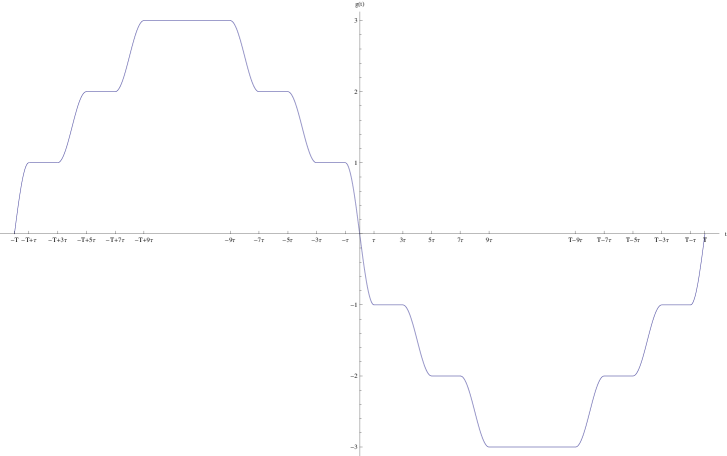
Figure 3: The sensitivity function $g_{3}(t)$ for the case of N=3 with the largest momentum transfer.

For a given time that the specific $\pi$ pulses are applied, there are six different sequences in all for the case of $N=3$. The schematics of the sensitivity functions of the other five sequences are presented in Fig.4. All the $30$ kinds of cases are summarized in the table 1. It is noted that there exist some interesting cases, e.g., $\Delta\Phi_{3}=0$ and this is impossible for the original interferometer consisted of beam splitter-mirror-beam splitter ($\frac{\pi}{2}-\pi-\frac{\pi}{2}$) optical pulse sequence. More interesting, for the sequence s6 and the time t1, $\Delta\Phi_{3}=-\frac{\omega_{a}}{c}gT^{2}$ which includes a reversed momentum recoil.

time/sequence	s1	s2	s3	s4	s5	s6
t1	$3\omega_{a}gT^{2}/c$	$\omega_{a}gT^{2}/c$	$\omega_{a}gT^{2}/c$	$\omega_{a}gT^{2}/c$	$\omega_{a}gT^{2}/c$	$-\omega_{a}gT^{2}/c$
t2	$2\omega_{a}gT^{2}/c$	$2\omega_{a}gT^{2}/c$	$0$	$2\omega_{a}gT^{2}/c$	$0$	$0$
t3	$2\omega_{a}gT^{2}/c$	$2\omega_{a}gT^{2}/c$	$2\omega_{a}gT^{2}/c$	$0$	$0$	$0$
t4	$\omega_{a}gT^{2}/c$	$\omega_{a}gT^{2}/c$	$\omega_{a}gT^{2}/c$	$\omega_{a}gT^{2}/c$	$\omega_{a}gT^{2}/c$	$\omega_{a}gT^{2}/c$
t5	$\omega_{a}gT^{2}/c$	$\omega_{a}gT^{2}/c$	$\omega_{a}gT^{2}/c$	$\omega_{a}gT^{2}/c$	$\omega_{a}gT^{2}/c$	$\omega_{a}gT^{2}/c$

Table 1: We list the results of the final leading phase shift for the structure of $N=3$. The rows refer to different sequences presented in Fig.4. The columns refers to different times, i.e. t1 and t2 have been indicated in the paper; t3:$\left(-T\right)\rightarrow\left(-T+3\tau\right)\rightarrow\left(-T+7\tau\right)\rightarrow\left(-T+11\tau\right)\rightarrow\left(-5\tau\right)\rightarrow\left(-\tau\right)\rightarrow\left(3\tau\right)\rightarrow\left(T-13\tau\right)\rightarrow\left(T-9\tau\right)\rightarrow\left(T-5\tau\right)\rightarrow\left(T-\tau\right)$; t4:$\left(-T\right)\rightarrow\left(-17\tau\right)\rightarrow\left(-13\tau\right)\rightarrow\left(-9\tau\right)\rightarrow\left(-5\tau\right)\rightarrow\left(-\tau\right)\rightarrow\left(3\tau\right)\rightarrow\left(7\tau\right)\rightarrow\left(11\tau\right)\rightarrow\left(15\tau\right)\rightarrow\left(T-\tau\right)$; t5:$\left(-T\right)\rightarrow\left(-T+3\tau\right)\rightarrow\left(-T+7\tau\right)\rightarrow\left(-T+11\tau\right)\rightarrow\left(-T+15\tau\right)\rightarrow\left(-\tau\right)\rightarrow\left(T-17\tau\right)\rightarrow\left(T-13\tau\right)\rightarrow\left(T-9\tau\right)\rightarrow\left(T-5\tau\right)\rightarrow\left(T-\tau\right)$.

Figure 4: The schematics of the sensitivity function for the interferometers with the other five sequences, respectively.

When the $N$ increases, the kinds of possible interferometers will increase. For example, when $N=4$, there are $140$ kinds with $20$ different sequences and $7$ different arrangements of the times for each sequence. Notably, for every kind of interferometer, there is only one structure to realize the largest momentum transfer, i.e. the final leading order phase shift is $N\omega_{a}gT^{2}/c$.

It has to be pointed out that when the LMT interferometers amplify the signal, the noises are also amplified simultaneously, which attenuates the advantage of such interferometers. This can be seen easily from the white phase noise, and here we present a result from the vibration noises. Fig.5 is a vibration spectrum measured in our lab. Assume such vibration happens in the measurement process of an interferometer, and we could estimate its influence on the final population change of atoms using the Eq. (17) of the appendix1, i.e. for the interferometer using three pulses described in the last section, the estimation of its influence is $\sim 2.99\times 10^{-7}$; for the interferometer of $N=3$ described in this section, the estimation is $\sim 1.18\times 10^{-6}$. It is seen easily that the influence of the vibration noise is amplified to nearly 4 times the previous one.

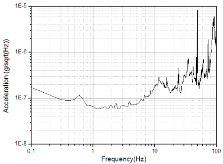
Figure 5: The spectrum of the vibration measured in our lab.

IV Configuration for the detection of gravitational waves

Although the new interferometers with LMT amplify noises existed in the process of the interferometry, many of the noises will be cancelled when the two new interferometers are operated in a proper method, as in the case of the detection of gravitational waves yt10 . Compared with the above discussion, the influence of vibration noise is $\sim 2.9\times 10^{-11}$ for the configuration with the baseline $L=1000$ km, which presents a very large suppression. See the schematic in Fig.6, and the consideration is similar to the Refs. yt10 ; ghkr13 , with the atomic interferometers replaced by the new interferometers discussed in the last section. The laser emitter is laid at the left side and the secondary pulse is formed by the reflection from the mirror fixed at the right side. In particular, the time interval between the primary and secondary pulses depends on the distance between the mirror and the right interferometer.

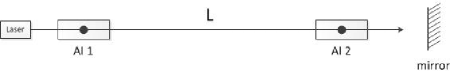
Figure 6: The schematic of the detector of gravitational waves with the use of the new interferometers.

The related noise analysis had been made in Refs. dgr08 ; ghkr13 . In particular, Ref. ghkr13 pointed out a remarkable point that the configuration is immune to laser frequency noise for the detection scheme of gravitational waves with the use of the new interferometers. Here we find some subtle differences, which will be discussed below, e.g. the suppression of the laser frequency noise is different between the cases of $N$ being even and odd, for the case with the largest momentum transfer (in the section we will only refer to the case with the largest momentum transfer, except a specific one is pointed out explicitly).

Firstly, we discuss the case for which $N$ is even, and assume that $N=2$ without loss of generality. This case had been introduced in the FIG.2 of Ref. ghkr13 with a $2\hbar k$ momentum transfer, in which the phase change due to the interaction of the laser with the atom can be expressed as

$$\Phi_{L}=\phi_{1}+\phi_{2}-\phi_{3}-2\phi_{4}-\phi_{5}+\phi_{6}+\phi_{7},$$

where the subscripts are associated with the seven pulses in chronological sequence. Now we consider the phase change caused by the phase fluctuation $\phi\left(t\right)$ which is due to the laser instability (here we ignore the other noise sources such as the fluctuation from atomic coherence), where $t$ means the time that the pulse is emitted from the laser emitter since the phase of a laser does not evolve during its propagation in vacuum. A direct intuition is to use the TDI to cancel the laser frequency noise, which is also mentioned in Ref. ghkr13 , but we find this is not feasible for the present scheme. Similar to the Ref. yt10 , the responses $R\left(t\right)$ of the new atomic interferometers to the laser phase noise can be written as

$$R_{21}\left(t\right) =\phi\left(t\right)+\phi\left(t-3\tau-L\right)-\phi\left(t-T+5\tau\right)-2\phi\left(t-T+\tau-L\right)$$

$$-\phi\left(t-T-3\tau\right)+\phi\left(t-2T+5\tau-L\right)+\phi\left(t-2T+\tau\right);$$ (6)

$$R_{22}\left(t\right) =\phi\left(t-L\right)+\phi\left(t-3\tau\right)-\phi\left(t-T+5\tau-L\right)-2\phi\left(t-T+\tau\right)$$

$$-\phi\left(t-T-3\tau-L\right)+\phi\left(t-2T+5\tau\right)+\phi\left(t-2T+\tau-L\right),$$ (7)

where for brevity we take $c=1$, $t$ is chosen at the time that the final laser is emitted, and “$2$” in the subscripts of $R_{21}\left(t\right)$ represents the case of $N=2$ and “$1$” represents the left interferometer in Fig.6. In particular, the subscripts of $\phi$ are omitted, because the laser frequency noise is only caused by the laser emitter and thus derives from the same function $\phi\left(t\right)$. If the laser is emitted from the left, the time of interaction between the laser and atoms in the right interferometer is delayed by $\Delta t=L$, and vice versa. By using the method of TDI, it was expected that $\Delta R\left(t\right)=R_{21}\left(t-L\right)-R_{22}\left(t\right)=0$, but actually it is not true for the case we are discussing, because a calculation gives $\Delta R\left(t\right)\neq 0$ by using the expressions (6) and (7). This is because for the present scheme, not all the laser pulses are emitted from the same direction, which is different from the situation discussed in Ref. yt10 . However, we find that, when $\tau$ is small enough compared with $L$ and $T$ (e.g. in a proposed experiment of Ref. ghkr13 , $\tau=20\mu$s, $L=1000$km or $3$ms, $T=1.5$s), the response functions can be written as

$$R_{21}\left(t\right) =\phi\left(t\right)+\phi\left(t-L\right)-\phi\left(t-T\right)-2\phi\left(t-T-L\right)$$

$$-\phi\left(t-T\right)+\phi\left(t-2T-L\right)+\phi\left(t-2T\right);$$ (8)

$$R_{22}\left(t\right) =\phi\left(t-L\right)+\phi\left(t\right)-\phi\left(t-T-L\right)-2\phi\left(t-T\right)$$

$$-\phi\left(t-T-L\right)+\phi\left(t-2T\right)+\phi\left(t-2T-L\right).$$ (9)

It is found directly that $\delta R(t)=R_{21}\left(t\right)-R_{22}\left(t\right)=0$. So one doesn’t need to consider any time delay, since the laser frequency noise can be cancelled at any time. Note that the cancellation is subtle, e.g. the first term of $R_{21}\left(t\right)$ is canceled by the second term of $R_{22}\left(t\right)$. This shows that the cancellation is better when the time internal is shorter (it is best for no time internal as the presentation in Ref. ghkr13 where the primary laser is triggered at time $t=0$, and the secondary one at time $t=L/c$ without any time internal). This result can also be extended to any case for which $N$ is even, since in that case, the number of laser pulses from one direction is equal to that from the other one.

However, we find the case for which $N$ is odd, is not the same. We show this by using the case of $N=3$ presented in Fig.2, and its responses $R\left(t\right)$ of the new atomic interferometers to the laser phase noise can be expressed as

$$R_{31}\left(t\right) =\phi\left(t\right)+\phi\left(t-3\tau-L\right)+\phi\left(t-7\tau\right)-\phi\left(t-T+9\tau\right)-\phi\left(t-T+5\tau-L\right)$$

$$-2\phi\left(t-T+\tau\right)-\phi\left(t-T-3\tau-L\right)-\phi\left(t-T-7\tau\right)+\phi\left(t-2T+9\tau\right)$$

$$+\phi\left(t-2T+5\tau-L\right)+\phi\left(t-2T+\tau\right)$$ (10)

$$R_{32}\left(t\right) =\phi\left(t-L\right)+\phi\left(t-3\tau\right)+\phi\left(t-7\tau-L\right)-\phi\left(t-T+9\tau-L\right)-\phi\left(t-T+5\tau\right)$$

$$-2\phi\left(t-T+\tau-L\right)-\phi\left(t-T-3\tau\right)-\phi\left(t-T-7\tau-L\right)+\phi\left(t-2T+9\tau-L\right)$$

$$+\phi\left(t-2T+5\tau\right)+\phi\left(t-2T+\tau-L\right).$$ (11)

Again it is found that $\Delta R\left(t\right)=R_{31}\left(t-L\right)-R_{32}\left(t\right)\neq 0$ even though small $\tau$ is considered. In particular, it is also found that $\delta R(t)=R_{31}\left(t\right)-R_{32}\left(t\right)\neq 0$ when the time internal $\tau$ is ignored; this is seen as

$$\delta R(t)=\phi\left(t\right)-\phi\left(t-L\right)-2\left(\phi\left(t-T\right)-\phi\left(t-T-L\right)\right)+\phi\left(t-2T\right)-\phi\left(t-2T-L\right)\text{.}$$

As expected, $\delta R(t)$ is very small since $\phi\left(t\right)$ is a slowly varying function which is required for any laser emitter. On the other hand, since $T>>L$, we might have $\delta R(t)=0$ by omitting the time internal $L$. That is permitted if it is within the sensitivity of the interferometer. But for the detection of gravitational waves, it is expected to remain the influence happened in the time internal $L$ since the signal is proportional to the length $L$. It is found that the reason that laser frequency noise cannot be cancelled exactly for any case with $N$ being odd is due to the asymmetry of the number of laser pulses from the two directions. However, the laser frequency noise is suppressed to a large extent, in the scheme with LMT.

Finally, we will point out the difference of $\Delta R\left(t\right)$ and $\delta R(t)$ operationally. $\Delta R\left(t\right)$ means that for each interaction, the pulse is the same for the first and the second interferometer. Such operation is easy to be understood physically for the measurement of gravitational waves. In particular, it also gets a large suppression of laser frequency noise in the present scheme. The reason that we use $\delta R(t)$ is that it leads to a complete cancellation of the laser frequency noise for the cases of even $N$. But for a single interaction, such operation means the pulses used to interact with the atoms are different for the first and second interferometers. Of course, it is only a choice of a proper data processing method dam , but we have to explain whether such operation can give the signal of gravitational waves. Fortunately, the latter operation will not change the signal since the response of the first interferometer to the gravitational waves, $R_{GW}(t)$, is usually treated as zero yt10 . Thus $\delta R_{GW}(t)=R_{1GW}(t)-R_{2GW}(t)=$ $R_{1GW}(t-L)-R_{2GW}(t)=$ $\Delta R_{GW}\left(t\right)$.

V Conclusion

In this paper we have investigated the sensitivity function and applied it to the transfer of the signal about gravitational field around the Earth through an atomic interferometer. We have also extended the application of sensitivity function to a new atomic interferometer for which we have analyzed its configuration in detail. In our analysis, we found that given the number of laser pulses, there are some different methods to realize LMT although the transferred momenta in each method are different. In particular, there is only one method that can realize the largest momentum transfer (i.e. $N\hbar k$ momenta transfer for a scheme with the specific $N$ defined in the paper), and in all these methods there are some configurations that gives the results of zero momentum transfer and even inverse momentum transfer (e.g. the final leading phase shift is $0$ or $-\frac{\omega_{a}}{c}gT^{2}$). For the configuration in Fig.6 for the detection of gravitational waves, we have also analyze how the laser frequency noise is cancelled. We found that when $N$ is even, the configuration is immune to the laser frequency noise with a proper data processing method; when $N$ is odd, the configuration only gives a large suppression for the laser frequency noise. However, for the present situation of detection scheme of gravitational waves, the use of new atomic interferometers with LMT is still a good progress for the amelioration of the laser frequency noise.

VI Acknowledgements

Financial support from NSFC under Grant Nos. 11104324, 11374330 and 11227803, and NBRPC under Grant Nos.2010CB832805 is gratefully acknowledged.

VII Appendix1

In the appendix, we will introduce briefly the transfer function.

In the paper, we used the sensitivity function to analyze the structure of an interferometer, but actually, maybe a little surprised, it is noted that when we choose $t_{i}=-T-\tau$ and $t_{f}=T+\tau$, the expression of the sensitivity function becomes

$$g_{c}(t)=\left\{\begin{array}[c]{c}\cos\Omega(T+t)\ \ \ \ ,-T-\tau\leqslant t<-T\\ \ 1\ \ \ \ \ \ \ \ \ \ \ \ \ \ ,-T\ \leqslant t<-\tau\\ -\sin\Omega t\ \ \ \ \ \ \ \ \ ,-\tau\leqslant t<\tau\\ -1\ \ \ \ \ \ \ \ \ \ \ \ \ ,\tau\leqslant t<T\\ -\cos\Omega(T-t)\ \ \ ,T\leqslant t\leqslant T\ +\tau\end{array}\right..$$ (12)

Thus if the initial time or the final time is chosen with a change of $\tau$, during that time the sensitivity function will change from sinusoidal to cosinusoidal function. This is easy to be known that such change is because we take $\Omega\tau=$ $\frac{\pi}{2}$. But the transfer function is nearly the same for the two different choices, which is a mathematical representation of the relation between the input and output of a measurement system and is also usually called the weighting function.

For the interferometer we considered here, the Fourier transform of the sensitivity function is

$$G\left(\omega\right)=\int_{-\infty}^{+\infty}e^{-i\omega t}g\left(t\right)dt.$$

and using sensitivity functions (2), we have

$$G\left(\omega\right)=\frac{4i\Omega^{2}}{\Omega^{2}-\omega^{2}}\sin\left(\frac{\omega T}{2}\right)\left[\frac{1}{\Omega}\cos\left(\frac{\omega T}{2}\right)+\frac{1}{\omega}\sin\left(\frac{\omega\left(T-2\tau\right)}{2}\right)\right].$$ (13)

In particular, for $\tau\ll T$, we have $G_{c}\left(\omega\right)\simeq G\left(\omega\right)$. Thus although our paper analyze the structure of the interferometers using the sensitivity function without discussing its dependence on the choice of the initial and final time, all results are applicable to any other analysis related to any change of the initial and final time.

Similarly, we can express the Fourier transform of the phase perturbation as $\Phi\left(\omega\right)=$ $\int_{-\infty}^{+\infty}e^{-i\omega t}\phi\left(t\right)dt$ and then put the reverse transform $\phi\left(t\right)=\int_{-\infty}^{+\infty}e^{i\omega t}\Phi\left(\omega\right)d\omega$ into Eq. (3). Thus we get

$$\Delta\Phi=-\int_{-\infty}^{+\infty}i\omega G\left(\omega\right)\Phi\left(\omega\right)d\omega.$$ (14)

Since the Fourier form $G\left(\omega\right)$ includes only a pure imaginary part seen from the Eq. (13), the interferometric phase is also written as $\Delta\Phi=\int_{-\infty}^{+\infty}\omega\left|G\left(\omega\right)\right|\Phi\left(\omega\right)d\omega$. After the introduction of the transfer function

$$H\left(\omega\right)=\omega G\left(\omega\right),$$ (15)

we have

$$\Delta\Phi=\int_{-\infty}^{+\infty}\left|H\left(\omega\right)\right|\Phi\left(\omega\right)d\omega,$$ (16)

which presents clearly the process how the interferometer responds to the phase disturbance (of course it also includes the signal). It is seen that if we put the Fourier transform of $\phi_{g}\left(t\right)$ into the Eq. (16), we can obtain the same result as Eq. (4). A notable feature of the transfer function $H\left(\omega\right)$ is a low pass first order filtering, having an oscillating behavior with a periodic frequency of $\delta\omega=\frac{2\pi}{T}$ but under the cutoff frequency $\omega_{c}=\frac{\sqrt{3}\Omega}{3}$ ccl05 .

However, the Eq. (16) is not usually used because most studies focused on the noise analysis while the power spectra of many noises are easier described, so the most popular is the variance of the phase fluctuation,

$$\sigma_{\Phi}^{2}=\int_{0}^{+\infty}\left|H\left(\omega\right)\right|^{2}S_{\phi}\left(\omega\right)d\omega$$ (17)

where $S_{\phi}\left(\omega\right)$ is the power spectral density of the phase perturbation and usually expressed as $S_{\phi}\left(\omega\right)=\left|\Phi\left(\omega\right)\right|^{2}$. It is stressed that $\sigma_{\Phi}^{2}$ is not related directly to the fluctuations of the interferometric phase, while related to the average value of $\Delta\Phi$. In particular, the average is usually taken for a long sequence of measurement cycles at a fixed repetition rate which will lead to an aliasing phenomenon similar to the Dick effect gjd87 in atomic clocks and increase the sensitivity of the interferometer on the low frequencies.

An immediate examination is to use the white phase noise with no frequency dependence, $S_{\phi}\left(\omega\right)=S_{\phi}^{0}$, and the result was given in the Ref. ccl05 and had a linear dependence on the inverse Raman pulse length. But the pulse length will affect the number of the participating atoms which leads to a shot noise and limits the sensitivity of the interferometer, so the optimum pulse length must be selected with the reference to the experimental parameters.

VIII Appendix2

In the appendix, we will give a detailed calculation for the sensitivity function of the interferometer presented in Fig.2.

Considering the atom which will go through the interferometer as a two-level system whose general state can be expressed as $\left|\varphi\left(t\right)\right\rangle=c_{a}\left(t\right)\left|a\right\rangle+c_{b}\left(t\right)\left|b\right\rangle$ with $\left|c_{a}\left(t\right)\right|^{2}+\left|c_{b}\left(t\right)\right|^{2}=1$, the evolution of the state under the interaction with the laser pulse is calculated with the change of the coefficients tr05 ,

$$c_{a}\left(t_{0}+\tau\right) =c_{a}\left(t_{0}\right)\cos\left(\frac{\Omega\tau}{2}\right)-ic_{b}\left(t_{0}\right)e^{i\phi}\sin\left(\frac{\Omega\tau}{2}\right),$$

$$c_{b}\left(t_{0}+\tau\right) =c_{b}\left(t_{0}\right)\cos\left(\frac{\Omega\tau}{2}\right)-ic_{a}\left(t_{0}\right)e^{-i\phi}\sin\left(\frac{\Omega\tau}{2}\right),$$ (18)

where $\Omega$ is the Rabi frequency, $\tau$ is the duration of the interaction, and $\phi$ is the relative phase change during the interaction.

For the case of $N=3$, there are eleven pulses, and in order to calculate the sensitivity function, except the phase $\phi_{0}$ carried by the pulses themselves which could be tuned in an experiment, a random phase change $\delta\phi$ during each interaction between the pulse and the atom may be introduced. For an illustration, we will calculate the result caused by the phase change $\delta\phi$ at time $t$ during the first pulse, $-T<t<-T+\tau$, by splitting the pulse into two pulses of duration $T+t$ and $-T+\tau-t$. We start by assuming all atoms in the state $\left|a\right\rangle$, and according to the sequence presented in Fig.2, the change of the coefficients after each pulse becomes,

$$c_{a1}(-T)=1,$$

$$c_{b2}(-T)=0;$$

$$c_{a1}(t)=\cos\frac{\Omega(t+T)}{2},$$

$$c_{b2}(t)=-ie^{-i\phi_{01}}\sin\frac{\Omega(t+T)}{2};$$

$$c_{a1}(-T+\tau) =c_{a1}(t-t-T+\tau)$$

$$=c_{a1}(t)\cos\frac{\Omega(\tau-t-T)}{2}-e^{i(\delta\phi+\phi_{01})}c_{b2}(t)\sin\frac{\Omega(\tau-T-t)}{2}$$

$$=\frac{\sqrt{2}}{2}(\cos^{2}\alpha+\sin\alpha\cos\alpha)-\frac{\sqrt{2}}{2}e^{i\delta\phi}(\sin\alpha\cos\alpha-\sin^{2}\alpha),$$

$$c_{b2}(-T+\tau)=-\frac{\sqrt{2}}{2}ie^{-i\phi_{01}}(\sin^{2}\alpha+\sin\alpha\cos\alpha)-\frac{\sqrt{2}}{2}ie^{-i(\phi_{01}+\delta\phi)}(\cos^{2}\alpha-\sin\alpha\cos\alpha),$$

where $\alpha=\frac{\Omega(t+T)}{2}$, $\Omega\tau=\frac{\pi}{2}$ for the first pulse with the change by a random phase $\delta\phi$, and the subscripts $a$, $b$ represent the two energy levels and 1, 2 represent the different paths. Since there is no new random phase introduced in the following ten pulses, the change of the coefficients is calculated easily according to the evolution (18). For the final pulse, we obtain the expression of $c_{a}$ as

$$c_{a}(T) =\frac{\sqrt{2}}{2}c_{a2}(T-3\tau)-\frac{\sqrt{2}}{2}ie^{i(\phi_{11}+\delta\phi)}c_{b1}(T-3\tau)$$

$$=-\frac{\sqrt{2}}{2}ie^{i(-\phi_{02}-\phi_{03}+\phi_{06}+\phi_{07}+\phi_{08}+\delta\phi)}c_{b}(-T+\tau)$$

$$-\frac{\sqrt{2}}{2}e^{i(\phi_{09}-\phi_{04}-\phi_{05}-\phi_{06}+\phi_{10}+\phi_{11})}c_{a}(-T+\tau)$$

$$=-\frac{1}{2}e^{i(-i\phi_{01}-\phi_{02}-\phi_{03}+\phi_{06}+\phi_{07}+\phi_{08}+\delta\phi)}(\sin^{2}\alpha+\sin\alpha\cos\alpha)$$

$$-\frac{1}{2}e^{i(-i\phi_{01}-\phi_{02}-\phi_{03}+\phi_{06}+\phi_{07}+\phi_{08})}(\cos^{2}\alpha-\sin\alpha\cos\alpha)$$

$$-\frac{1}{2}e^{i(\phi_{09}-\phi_{04}-\phi_{05}-\phi_{06}+\phi_{10}+\phi_{11})}(\cos^{2}\alpha+\sin\alpha\cos\alpha)$$

$$+\frac{1}{2}e^{i(\phi_{09}-\phi_{04}-\phi_{05}-\phi_{06}+\phi_{10}+\phi_{11}+\delta\phi)}(\sin\alpha\cos\alpha-\sin^{2}\alpha).$$

Define $\Phi=\phi_{01}+\phi_{02}+\phi_{03}-\phi_{04}-\phi_{05}-2\phi_{06}-\phi_{07}-\phi_{08}+\phi_{09}+\phi_{10}+\phi_{11}=\frac{\pi}{2}$, and we get the final probability of finding the atom still in state $\left|a\right\rangle$,

$$P_{a} =\left|c_{a}(T)\right|^{2}$$

$$=\frac{1}{4}[2+\cos\Phi(1+\cos 4\alpha+2\cos\delta\phi\sin^{2}2\alpha)+2\sin\Phi\sin 2\alpha\sin\delta\phi]$$

$$=\frac{1}{2}(1+\sin\Omega(t+T)\sin\delta\phi).$$

Thus according to the definition (1) of the sensitivity function, we have it in the time interval $-T<t<-T+\tau$ as

$$g(t)=\sin\Omega(t+T).$$

Then we can proceed in a similar way but the random phase change is introduced in other ten pulses to obtained the sensitivity functions for those time intervals, and thus the whole sensitivity function $g_{3}(t)$ is gotten as presented in the third section of this paper.

The transfer function can be obtained using (15),

$$H(\omega) =\frac{2\omega^{2}i}{\Omega^{2}-\omega^{2}}[\frac{\Omega}{\omega}\sin\omega T-\cos\omega(T-\tau)+\cos\omega\tau]+2i\sin\omega\tau[2\sin\omega(T-2\tau)$$

$$+3\sin\omega(T-4\tau)+4\sin\omega(T-6\tau)+5\sin\omega(T-8\tau)+5\sin 8\omega\tau+4\sin 6\omega\tau$$

$$+3\sin 4\omega\tau+2\sin 2\omega\tau]+12i\sin\frac{\omega(T-18\tau)}{2}\sin\frac{\omega T}{2}$$

$$+\frac{2\omega^{2}i}{\Omega^{2}-\omega^{2}}\cos\omega\tau[-\cos\omega(T-4\tau)-\cos\omega(T-8\tau)+\cos 8\omega\tau+\cos 4\omega\tau],$$

which is seen from the Fig.7.

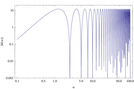
Figure 7: The transfer function H(w) which is the Fourier transform of the sensitivty function $g_{3}(t)$

References

- (1) J. R. Gair, M. Vallisneri, S. L. Larson, and J. G. Baker, Living Rev. Relativity 16, 7 (2013).
- (2) J. Weber, Phys. Rev. Lett. 22, 1320 (1969).
- (3) T. Accadia, F. Acernese, F. Antonucci, et al., J. Phys. Conf. Ser. 203, 012074 (2010).
- (4) B. P. Abbott, R. Abbott, R. Adhikar, et al., Rep. Prog. Phys. 72, 076901 (2009).
- (5) G. M. Harry (for the LIGO Scientific Collaboration), Class. Quantum Grav. 27, 084006 (2010).
- (6) E. Poisson, Phys. Rev. D 54, 5939 (1996).
- (7) The LIGO Scientific Collaboration and The Virgo Collaboration, Nature, 460, 990 (2009).
- (8) L. M. Krauss and F. Wilczek, arXiv: 1309.5343 [hep-th].
- (9) R. Y. Chiao and R. Y. Speliotopoulos, J. Mod. Opt., 51, 861 (2004).
- (10) R. Y. Speliotopoulos and R. Y. Chiao, Phys. Rev. D 69, 084013 (2004).
- (11) A. Roura, et al, Phys. Rev. D 73, 084018 (2006).
- (12) S. Dimopoulos, P. W. Graham, J. M. Hogan, M. A. Kasevich, and S. Rajendran, Phys. Rev. D 78, 122002 (2008).
- (13) S. Dimopoulos, P. W. Graham, J. M. Hogan, and M. A. Kasevich, Phys. Rev. D 78, 042003 (2008).
- (14) N. Yu and M. Tino, Gen. Relativ. Gravit. 43, 1943 (2011).
- (15) H. Mueller, S. Chiow, Q. Long, S. Herrmann, and S. Chu, Phys. Rev. Lett. 100, 180405 (2008).
- (16) P. W. Graham, J. M. Hogan, M. A. Kasevich, and S. Rajendran, Phys. Rev. Lett. 110, 171102 (2013).
- (17) P. Cheinet, B. Canuel, F. P. D. Santos, A. Gauguet, F. Leduc, and A. Landragin, submitted to IEEE Trans. on Instrum. Meas., Arxiv: physics/0510197 (2005).
- (18) M. A. Kasevich and S. Chu, Phys. Rev. Lett. 67 181 (1991).
- (19) M. A. Kasevich and S. Chu, Appl. Phys. B 54, 321 (1992).
- (20) P. Storey and C. Cohen-Tannoudji, J. Phys. France 4, 1999 (1994).
- (21) A. Peters, K. Y. Chung, B. Young, J. Hensley, and S. Chu, Phil. Trans. R. Soc. Lond. A 355, 2223 (1997).
- (22) B. Zhang, Q. Y. Cai, and M. S. Zhan, EPJD 67, 184 (2013).
- (23) D. S. Weiss, B. C. Young, and S. Chu, Appl. Phys. B 59, 217 (1994).
- (24) A. Peters, K. Y. Chung, and S. Chu, Metrologia 38, 25 (2001).
- (25) G. J. Dick, Local Oscillator induced instabilities, in Proc. Nineteenth Annual Precise Time and Time interval, 133-147 (1987).
- (26) It is stressed that the data processing method is only applicable for the cancellation of laser frequency noise and whether it is feasible for the suppression of other noises has to be analyzed independently and carefully.
- (27) T. Petelski, Ph.D Thesis, University of Firenze, Italy, 2005.