Abstract

Using the non-equilibrium Green function method (Kadanoff-Baym equations) in the expanding universe, we investigate evolution of the lepton number asymmetry when the right-handed (RH) neutrinos have almost degenerate masses $|M_{i}^{2}-M_{j}^{2}|\ll M_{i}^{2}$. The resonantly enhanced $CP$-violating parameter $\varepsilon_{i}$ associated with the decay of the RH neutrino $N_{i}$ is obtained. It is proportional to an enhancement factor $(M_{i}^{2}-M_{j}^{2})M_{i}\Gamma_{j}/((M_{i}^{2}-M_{j}^{2})^{2}+R_{ij}^{2})$ with the regulator $R_{ij}=M_{i}\Gamma_{i}+M_{j}\Gamma_{j}$. The result is consistent with the previous result obtained by Garny et al., in a constant background with an out-of-equilibrium initial state. We discuss the origin of such a regulator, and why it is not like $R_{ij}=M_{i}\Gamma_{i}-M_{j}\Gamma_{j}$.

1 Introduction

Origin of the Baryon asymmetry in the universe is one of the unsolved issues in particle physics. Although the standard model (SM) satisfies the Sakharov’s three conditions [1], sufficient number of baryon asymmetry cannot be produced due to the smallness of the $CP$-asymmetry in the CKM matrices and the modest electroweek phase transition. On the other hand, the neutrino oscillation which implies tiny neutrino masses demands that some extension of the SM is necessary. Introducing right-handed (RH) neutrinos $N_{i}$ with large Majorana masses $M_{i}$ gives a natural solution to explain the smallness of the neutrino masses via see-saw mechanism, but it also naturally explain the Baryon number asymmetry in the universe through the leptogenesis [2]. (See e.g., a very nice recent review [3].) In this scenario, RH neutrinos are produced thermally by the reheating after inflation. As temperature decreases with the expansion of the universe down to the Majorana mass scale, RH neutrinos become out of thermal equilibrium and their $CP$-asymmetric decay into the SM leptons and the Higgs produce lepton number asymmetry in the universe. The lepton number asymmetry produced is then converted into the baryon number asymmetry through the nonperturbative $B+L$ -violating process of sphalerons in the SM [4].

If the Majorana masses of the RH neutrinos have a hierarchical structure, the lightest Majorana mass must satisfy the Davidson-Ibarra(DI) bound [5], $M\raisebox{-2.15277pt}{$\>\stackrel{{\scriptstyle\textstyle>}}{{\sim}}\>$}10^{9}$GeV in order to produce sufficient lepton number asymmetry. When at least two of the RH neutrinos are degenerate in their masses, the DI bound can be evaded. In this case, quantum oscillation of almost degenerate RH neutrinos resonantly enhance the $CP$-violating decay and hence lepton number asymmetry can be produced sufficiently even for RH neutrino masses as light as TeV scale. This scenario is known as the resonant leptogenesis [8] [9] [10]. Such light RH neutrinos might induce detectable non-unitarity of the mixing matrix of active neutrinos [11] [12] and have attracted much attention.

TeV scale leptogenesis has attracted enormous attention in light of the LHC experiment [13]–[40]. The scale can be made even smaller if the leptotenesis occurs through $CP$-violating oscillations between RH neutrinos far away from the thermal equilibrium. The mechanism plays an important role in the model of $\nu$MSM [41]–[45].

Furthermore, light RH neutrinos do not give large radiative corrections to the Higgs boson mass and are safe in view of the naturalness [46]. Related to the naturalness of the electroweak weak against higher physical scales, one of the authors proposed a classically conformal $U(1)_{B-L}$ extension of the SM [47] [48]. In this model, $B-L$ gauge symmetry is spontaneously broken via the Coleman-Weinberg mechanism which triggers the electroweak gauge symmetry. In [49], we further showed that if the Higgs potential is flat at the Planck scale, the model naturally predicts the Higgs boson mass at around 126 GeV and TeV scale $B-L$ breaking (or the leptogenesis). This motivated us to investigate the TeV scale leptogenesis in the $U(1)_{B-L}$ model [28].

In the resonant case, the $CP$-asymmetry in the decay of $N_{i}$ mainly comes from an interference of the tree and the self-energy one-loop diagrams (See Fig.1). It is expressed by the $CP$-violating parameter

$$\varepsilon_{i} \equiv\frac{\Gamma_{N_{i}\to\ell\phi}-\Gamma_{N_{i}\to\overline{\ell}\overline{\phi}}}{\Gamma_{N_{i}\to\ell\phi}+\Gamma_{N_{i}\to\overline{\ell}\overline{\phi}}}=\sum_{j(\neq i)}\frac{\Im(h^{{\dagger}}h)^{2}_{ij}}{(h^{{\dagger}}h)_{ii}(h^{{\dagger}}h)_{jj}}\frac{(M^{2}_{i}-M^{2}_{j})M_{i}\Gamma_{j}}{(M^{2}_{i}-M^{2}_{j})^{2}+R_{ij}^{2}}$$ (1.1)

where $h$ is the neutrino Yukawa coupling and $\Gamma_{i}\simeq(h^{{\dagger}}h)_{ii}M_{i}/8\pi$ is the decay width of $N_{i}$. The resonant enhancement of the $CP$-violating parameter was discussed in [50]. Systematic considerations were performed by Pilaftsis [9][51][52], and he found that the regulator in the denominator is given by $R_{ij}=M_{i}\Gamma_{j}$. If the mass difference is larger than the decay width, we have $|M^{2}_{i}-M^{2}_{j}|\gg R_{ij}$, and $\varepsilon_{i}$ is suppressed by $\Gamma_{i}/M\sim(h^{{\dagger}}h)_{ii}$. However, in the degenerate case, $|M_{i}-M_{j}|\sim\Gamma$ and $\varepsilon$ can be enhanced to ${\mathcal{O}}((h^{\dagger}h)^{0})\sim 1$. Hence the determination of the regulator $R_{ij}$ is essential for a precise prediction of the lepton number asymmetry in the resonant leptogenesis. The authors [53] calculated the resummed propagator of the RH neutrinos and obtained a different regulator $R_{ij}=|M_{i}\Gamma_{i}-M_{j}\Gamma_{j}|$. By using their result, the enhancement factor becomes much larger. The origin of the difference of the regulators is discussed in [54] [55]. Since the lower scale of the leptogenesis is strongly sensitive to the form of the regulator, it is very important to systematically evaluate the precise form of the regulator.

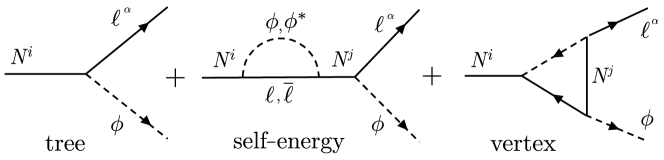
Figure 1: Tree and one-loop diagrams of the RH neutrino decay. In the resonant case, an interference of the tree and the self-energy diagram [6] [7] gives a dominant contribution to the $CP$-violating parameter.

Conventionally, leptogenesis is often calculated based on the classical Boltzmann equation which describes the time evolution of the phase space distribution function of on-shell particles [85]. In the Boltzmann equation, the interactions between particles are taken into account through the collision terms that comprise the $S$-matrix elements calculated separately in the framework of quantum field theory. The authors [57] applied the non-equilibrium Green’s function method with the Kadanoff-Baym (KB) equations developed in studies of the transport phenomena [87][88] and derived the full-quantum evolution equation for the lepton number in the hierarchical mass case. Using this method, one can systematically take into account quantum interference, finite temperature and finite density effects. The method was intensively used in the leptogenesis in various papers [58]–[69]. In the resonant leptogenesis, since the quantum interference effect is crucial to the evaluation of the $CP$-violating parameter, we can expect importance of such a full-quantum mechanical formulation based on the KB equations. In [70], the authors used the method to obtain an oscillating $CP$-violating parameter in the flat space-time. Then applying it to the Boltzmann equation in the expanding universe, they calculated the lepton number asymmetry. In the strong washout regime, the oscillation is averaged out and the lepton number asymmetry is expressed with an effective $CP$-violating parameter. Then the maximal value agrees with the case of $R_{ij}=M_{i}\Gamma_{j}$[71]. The authors of [72] also found an oscillatory behavior by a different calculation, and discussed an implication to the leptogenesis in the expanding universe. The quantum oscillations in the flavored leptogenesis was also performed in [73][74][75].

Recently Garny et al. [56] systematically investigated generation of the lepton asymmetry in the resonant leptogenesis using the formulas developed in [58][59]. In the investigation, they considered a non-equilibrium initial condition in a time-independent background and calculated generation of the lepton number asymmetry. Starting from the vacuum initial state for the RH neutrinos, they read off the $CP$-violating parameter from the generated lepton number asymmetry. The effective regulator they derived is $R_{ij}=M_{i}\Gamma_{i}+M_{j}\Gamma_{j}$, which differs from the previous results, $R_{ij}=M_{i}\Gamma_{j}$ by [9] or $R_{ij}=|M_{i}\Gamma_{i}-M_{j}\Gamma_{j}|$ by [53].

The purpose of the present paper is to perform systematic investigations of the thermal resonant leptogenesis based on the KB equations. We scrutinize various properties of the Green functions of the RH neutrinos, and directly extract the $CP$-violating parameter $\varepsilon_{i}$ from the evolution equation for the lepton number in the expanding universe, with an emphasis on the quantum flavor oscillations.

The paper is organized as follows. In section 2.1 and 2.2, we first summarize the basic properties of various Green functions and the Kadanoff-Baym (KB) equations that these Green functions must satisfy. Then we derive the evolution equation of the lepton number in the expanding universe in section 2.3. The evolution equation is written in terms of the propagators of the RH neutrinos, the SM leptons and the Higgs. In section 2.4 we explain how the KB equation is reduced to the ordinary Boltzmann equation. The most important ingredient necessary to solve the evolution equation for the lepton number is the Wightman functions of the RH neutrinos. The flavor diagonal component is directly related to the distribution function, but more important for the lepton asymmetry is its off-diagonal component.

In section 3, we investigate how the flavor oscillation affects the off-diagonal component of the propagators. In the section, we focus on the resonant oscillations in the thermal equilibrium. In section 3.1, 3.2 and 3.3, we study the properties of the retarded and advanced propagators in which information of the spectrum is encoded. Then we study the Wightman functions with information of the distribution functions.

In section 4, we scrutinize the behavior of Green functions out of equilibrium. In the expanding universe, Green functions are approximated in the leading order approximation by the thermal values at the local temperature. But in order to calculate the lepton asymmetry, deviations from the thermal values are important. We show in section 4.3 that the deviations of the flavor off-diagonal Wightman functions from the thermal values behave quite differently from behaviors of other Green functions.

In section 5, we apply the calculated deviations of the Wightman functions of the RH neutrinos into the evolution equation derived in section 2, and obtain the quantum Boltzmann equation for the lepton number asymmetry. The deviations are classified into 3 types. One of them generate the lepton number asymmetry while the other two wash out the generated asymmetry. In section 5.4, we read off the $CP$-violating parameter $\varepsilon$ and show that the regulator is given by $R_{ij}=M_{i}\Gamma_{i}+M_{j}\Gamma_{j}$.

In section 6, we give a physical interpretation why the regulator $R_{ij}=M_{i}\Gamma_{i}+M_{j}\Gamma_{j}$ appears instead of $R_{ij}=M_{i}\Gamma_{i}-M_{j}\Gamma_{j}$. In particular, we show that if we neglect what we call the off-shell contributions the regulator is erroneously given by $R_{ij}=M_{i}\Gamma_{i}-M_{j}\Gamma_{j}$.

In section 7, we summarize our results.

In appendix A and B, we give a brief introduction to the closed time path (CTP) formalism and the KB equations. In appendix C, we introduce the 2PI formalism and then in appendix D we derive the self-energies for the RH neutrinos and the SM leptons based on the 2PI formalism. In appendix E and F, some useful identities in calculating convolutions are given. From appendix G to J, we give details of the calculations of various Green functions. In appendix K, we give anther derivation of the off-diagonal component of the Wightman functions out of equilibrium. The calculation explains why the regulator $R_{ij}=M_{i}\Gamma_{i}+M_{j}\Gamma_{j}$ naturally appears. Appendices L and M are calculations of some equations in the paper.

2 Evolution equations of lepton numbers

A systematic method to investigate the evolution of lepton asymmetry is the Kadanoff-Baym (KB) equations. The advantage of the KB equation to the Boltzmann equation is that it gives a quantum evolution equation of various correlation functions which does not distinguish on-shell and off-shell states. Accordingly it can take into account quantum coherence of the system and memory effects. Also the doubling problem in the scattering processes with on-shell internal lines can be systematically resolved (see [68] and references therein). The KB equation can be reduced to the classical Boltzmann equation only in special cases where the memory effects can be neglected.

Time-evolution of a quantum system is determined by the Hamiltonian of the system and the initial wave function at the initial time $t=t_{i}$. Such time-evolution is described by the wave function at later times, or instead, a set of all $n$-point Green functions. Of course, it is practically impossible to study the evolution equations containing all the $n$-point functions and we need to select an important set of observables. In the classical approach based on the Boltzmann equation, one-particle distribution function on the phase space is selected. In the quantum Boltzmann approach, two-point Green functions are selected.

In this section, we summarize notations of various Green functions and their basic properties in the thermal equilibrium. We also summarize the non-equilibrium evolution equation (KB equation) for the Green functions. More details are given in Appendices. After brief reviews in section 2.2 and 2.3, we derive the evolution equation of the lepton number in section 2.4 and 2.5.

2.1 Our model

The model we consider is an extension of the SM with RH neutrinos $\nu_{R,i}$. $i$ is the flavor index, $i=1,2,3.$ We set $N_{i}=\nu_{R,i}+\nu_{R,i}^{c}$. The Lagrangian is given by

$${\mathcal{L}}={\mathcal{L}}_{SM}+\frac{1}{2}\overline{N}^{i}(i{\ooalign{\hfil/\hfil\crcr$\nabla$}}-M_{i})N^{i}+{\mathcal{L}}_{int}\ ,$$ (2.3)

$${\mathcal{L}}_{int}\equiv-h_{\alpha i}(\overline{\ell}^{\alpha}_{a}\epsilon_{ab}\phi^{*}_{b})P_{R}N^{i}+h^{{\dagger}}_{i\alpha}\overline{N}^{i}P_{L}(\phi_{b}\epsilon_{ba}\ell^{\alpha}_{a})$$ (2.4)

where $\alpha,\beta=1,2,3$ and $a,b=1,2$ are flavor indices of the SM leptons $\ell_{a}^{\alpha}$ and isospin $SU(2)_{L}$ indices respectively. $M_{i}$ is the Majorana mass of $N_{i}$ and $h_{i\alpha}$ is the Yukawa coupling of $N^{i},\ell_{a}^{\alpha}$ and the Higgs $\phi_{a}$ doublet. $P_{R(L)}$ are chiral projections on right(left)-handed fermions. In the present paper, we consider the case of almost degenerate Majorana masses at TeV scale. Then the Yukawa couplings become very small $h_{i\alpha}\ll 1$ so as to generate tiny neutrino masses through the see-saw mechanism. Hence the decay width $\Gamma_{i}\simeq(h^{{\dagger}}h)_{ii}M_{i}/8\pi$ is much smaller than the mass $M_{i}$.

2.2 Green functions and KMS relations

Various Green functions are introduced in field theories. Consider a fermion field $\psi$. The statistical propagator $G_{F}$ and the spectral density $G_{\rho}$ are defined as

$$G_{F}(x,y)= \frac{1}{2}\langle[\hat{\psi}(x),\overline{\hat{\psi}}(y)]\rangle\ ,$$ (2.5)

$$G_{\rho}(x,y)= i\langle\{\hat{\psi}(x),\overline{\hat{\psi}}(y)\}\rangle\ .$$ (2.6)

The statistical propagator $G_{F}$ contains information of the particle density of the state on which operators are evaluated. On the other hand, the spectral density $G_{\rho}$ gives information of the particle’s mass and decay width. Because of the anti-commutator, $\gamma^{0}G_{\rho}(x^{0},y^{0})$ becomes proportional to the spatial delta function $\delta^{3}({\bf x}-{\bf y})$ at the equal time $x^{0}=y^{0}$:

$$\gamma_{0}G_{\rho}(x,y)=i\delta^{3}({\bf x}-{\bf y}){\bf 1}$$ (2.7)

where ${\bf 1}$ is an identity matrix in the flavor and the spinor indices.

Other useful Green functions are the Wightman functions

$$G_{>}(x,y)= G_{F}(x,y)-\frac{i}{2}G_{\rho}(x,y)=\langle\hat{\psi}(x)\overline{\hat{\psi}}(y)\rangle\ ,$$ (2.8)

$$G_{<}(x,y)= G_{F}(x,y)+\frac{i}{2}G_{\rho}(x,y)=-\langle\overline{\hat{\psi}}(y)\hat{\psi}(x)\rangle$$ (2.9)

and the retarded and advanced Green functions are given by

$$G_{R/A}(x,y)= \pm{\rm\Theta}(\pm(x^{0}-y^{0}))G_{\rho}(x,y)\ .$$ (2.10)

The spectral function can be written as $G_{\rho}=G_{R}-G_{A}=i(G_{>}-G_{<})$.

In the present paper, we assume homogeneity along the spatial directions so that we can always use the Fourier transform in the 3-dimensional space. If the state is described by the thermal equilibrium state, we can further Fourier transform in the time direction. In the thermal equilibrium at temperature $T$, the Green functions $G(x,y)$ are anti-periodic in the time direction with an imaginary period $i\beta=i/T$ and their Fourier transforms satisfy the KMS (Kubo Martin Schwinger) relation

$$G^{(eq)}_{\tiny\raisebox{-0.5pt}[0.0pt][0.0pt]{$\stackrel{{\scriptstyle\textstyle>}}{{\textstyle\rule{0.0pt}{1.5pt}\smash{<}}}$}}(q)=-i\left\{\begin{matrix}1-f(q_{0})\\ -f(q_{0})\end{matrix}\right\}G^{(eq)}_{\rho}(q)\ ,\ \ G^{(eq)}_{F}(q)=-i\left(\frac{1}{2}-f(q_{0})\right)G^{(eq)}_{\rho}(q)\ .$$ (2.11)

Here $f(q_{0})$ is the Fermi-Dirac distribution function $f(q_{0})=1/(e^{q_{0}/T}+1).$ In presence of the chemical potential $\mu$, $q_{0}$ is replaced by $q_{0}-\mu$. Since the relation relates the fluctuation described by the Wightman function to the dissipation described by the retarded Green function, it is also called the fluctuation-dissipation relation. By this relation, the spectrum of the system determines all the Green functions. When the system becomes out of equilibrium, the KMS relation is violated. The violation plays an important role in the leptogenesis.

As a final remark in this section, let us recall that the explicit forms of the Wightman functions of free charged fermions (bosons) are given by

$$G_{\tiny\raisebox{-0.5pt}[0.0pt][0.0pt]{$\stackrel{{\scriptstyle\textstyle>}}{{\textstyle\rule{0.0pt}{1.5pt}\smash{<}}}$}}^{{\rm free}}(x,y)=\int\frac{d^{3}q}{(2\pi)^{3}}e^{+i{\mathbb{q}}\cdot({\mathbb{x}}-{\mathbb{y}})}\frac{1}{2\omega_{q}}$$

$$\times{\Big{[}}e^{-i\omega_{q}(x^{0}-y^{0})}\left\{\begin{matrix}1-\eta f_{\mathbb{q}}\\ -\eta f_{\mathbb{q}}\end{matrix}\right\}\hat{g}_{+}+e^{+i\omega_{q}(x^{0}-y^{0})}\left\{\begin{matrix}-\eta\bar{f}_{-{\mathbb{q}}}\\ 1-\eta\bar{f}_{-{\mathbb{q}}}\end{matrix}\right\}\hat{g}_{-}{\Big{]}}$$ (2.12)

where $\omega_{q}$ is the energy of the on-shell particle, and $\hat{g}_{\pm}=(\pm\omega_{q}\gamma^{0}-{\mathbb{q}}\cdot{\boldsymbol{\gamma}}+m)$, $\eta=+1$ for Dirac fermions with their mass $m$ and $\hat{g}_{\pm}=1$, $\eta=-1$ for bosons. $f_{\mathbb{q}}$ and $\bar{f}_{\mathbb{q}}$ are distribution functions of on-shell particles and anti-particles with their spatial momentum ${\mathbb{q}}$ respectively. They are not necessarily the equilibrium distribution functions.

2.3 Kadanoff-Baym equations

If the system is out of equilibrium and the state is time-dependent, we cannot use the ordinary perturbative method based on the Feynmann propagators. A general formalism is given by the closed-time-path (CTP) formalism in which perturbative vertices are inserted on the closed-time-path ${\mathcal{C}}={\mathcal{C}}_{+}+{\mathcal{C}}_{-}.$ See Appendix A for brief review and Figure 4 there. One of the self-consistent approximation of the Schwinger-Dyson equations in the CTP formalism is called Kadanoff-Baym (KB) equation. Derivation of the KB equations is given in Appendix B and C.

The equations for the retarded and advanced Green functions are

$$iG_{0(x)}^{-1}G_{R/A}(x,y)-\int^{\infty}_{t_{int}}d^{4}z_{g}\ \Pi_{R/A}(x,z)G_{R/A}(z,y)=-\delta^{g}(x-y)\ .$$ (2.13)

Here $d^{4}z_{g}$ is an abbreviation of $d^{4}z\sqrt{-g(z)}$ and $\delta^{g}(x-y)=\delta^{4}(x-y)/\sqrt{-g}$. $G_{0(x)}^{-1}$ is the free kinetic operator whose derivatives act on a field at $x$. $\Pi_{R/A}$ is the self-energy and defined in eq.(B.21). They have the same properties as $G_{R/A}$, e.g., $\Pi_{R}(x,y)=0$ for $x^{0}<y^{0}$ is satisfied. Note that the integration range in (2.13) is constrained between $x_{0}$ and $y_{0}$:

$$\int^{x^{0}(y^{0})}_{y^{0}(x^{0})}d^{4}z_{g}\ \Pi_{R/A}(x,z)G_{R/A}(z,y)$$ (2.14)

because of the step functions in $\Pi_{R/A}$ and $G_{R/A}$. Therefore $G_{R/A}(x,y)$ is determined by the local information between $x_{0}$ and $y_{0}$. Namely $G_{R/A}$ does not depend on the information of the system in the past: there is no memory effect for $G_{R/A}$.

Other Green functions $G_{*}$ ($*=F,\rho,\lessgtr$) satisfy

$$iG_{0(x)}^{-1}G_{*}(x,y) = \int^{\infty}_{t_{int}}d^{4}z_{g}\ \Pi_{R}(x,z)G_{*}(z,y)+\int^{\infty}_{t_{int}}d^{4}z_{g}\ \Pi_{*}(x,z)G_{A}(z,y)$$

$$= \int^{x^{0}}_{t_{int}}d^{4}z_{g}\ \Pi_{R}(x,z)G_{*}(z,y)+\int^{y^{0}}_{t_{int}}d^{4}z_{g}\ \Pi_{*}(x,z)G_{A}(z,y)\ .$$ (2.15)

In the second equality, we have used the properties of $R/A$ functions. By using eq.(2.13), this equation can be solved formally in terms of the self-energy function and the $R/A$ Green functions as

$$G_{*}(x,y) = -\int_{t_{int}}^{\infty}d^{4}z_{g}d^{4}w_{g}G_{R}(x,z)\Pi_{*}(z,w)G_{A}(w,y)$$ (2.16)

$$\equiv -(G_{R}*\Pi_{*}*G_{A})(x,y)\ .$$

In the last line $*$-operation denotes the convolution operation.

Let us see the memory effect of $G_{*}$. Generally speaking, the integrals in (2.15) over $z$ are performed from the past at the initial time $t_{int}$ to $x^{0}$ or $y^{0}$. This makes Green functions dependent on the state of the system in the past before $x^{0}$ or $y^{0}$. This is indeed the case for $G_{F}$ and $G_{\lessgtr}$, but for the spectral density $G_{\rho}$, there is no memory effect. It can be seen by using $\Pi_{\rho}=\Pi_{R}-\Pi_{A}$. Then the integral of (2.15) can be rewritten as

$$iG_{0(x)}^{-1}G_{\rho}(x,y)=\int^{x^{0}}_{y^{0}}d^{4}z_{g}\ \Pi_{\rho}(x,z)G_{\rho}(z,y)\ .$$ (2.17)

Or it can be directly seen from the relation $G_{\rho}=G_{R}-G_{A}$. The relation $G_{\rho}=-G_{R}\Pi_{\rho}G_{A}=G_{R}-G_{A}$ is equivalent to $\Pi_{\rho}=\Pi_{R}-\Pi_{A}=G_{R}^{-1}-G_{A}^{-1}.$

In the thermal equilibrium, since the system is translationally invariant, (2.16) can be Fourier transformed and

$$G_{*}^{(eq)}(p)=-G_{R}^{(eq)}(p)\Pi_{*}^{(eq)}(p)G_{A}^{(eq)}(p)\ .$$ (2.18)

These equations (2.13), (2.15) are not closed within the two-point Green functions because the self-energy $\Pi$ contains $n(>2)$-point functions. Hence, in order to solve them explicitly, we need to make an approximation to express $n(>2)$-point functions in terms of the two-point functions. 2PI effective action method is one of the simplest and self-consistent methods. (See Appendix C for brief explanation.) By using it, the self-energies $\Pi$ in the above equations (2.13) (2.15) are represented as a sum of 1PI diagrams made of full propagators, and consequently these equations can be interpreted as simultaneous equations for various propagators in the system. These self-consistent equations among the propagators are especially called the Kadanoff-Baym equations.

2.4 Evolution of lepton number in the expanding universe

Now we investigate the KB equations of lepton numbers in the expanding universe. We first define Green functions, $G$, $S$ and $\Delta$ for the RH neutrinos, the SM lepton doublet and the Higgs doublet respectively:

$$G_{>}^{ij}(x,y)=\langle\hat{N}^{i}(x)\overline{\hat{N}}^{j}(y)\rangle\ , \ \ G^{ij}_{<}(x,y)=-\langle\overline{\hat{N}}^{j}(y)\hat{N}^{i}(x)\rangle\ ,$$ (2.19)

$$S^{\alpha\beta}_{ab>}(x,y)=\langle\hat{\ell}^{\alpha}_{a}(x)\overline{\hat{\ell}}^{\beta}_{b}(y)\rangle\ , \ \ S^{\alpha\beta}_{ab<}(x,y)=-\langle\overline{\hat{\ell}}^{\beta}_{b}(y)\hat{\ell}^{\alpha}_{a}(x)\rangle\ ,$$ (2.20)

$$\Delta_{ab>}(x,y)=\langle\hat{\phi}_{a}(x)\hat{\phi}^{{\dagger}}_{b}(y)\rangle\ , \ \ \Delta_{ab<}(x,y)=+\langle\hat{\phi}^{{\dagger}}_{b}(y)\hat{\phi}_{a}(x)\rangle\ .$$ (2.21)

The classical inverse propagators are given by

$$iG_{0}^{-1\ ij}(x,y)= (i{\ooalign{\hfil/\hfil\crcr$\nabla$}}_{x}-M_{i})\delta^{ij}\delta^{g}(x-y)\ ,$$ (2.24)

$$iS_{0\ \ \ ab}^{-1\ \alpha\beta}(x,y)= i{\ooalign{\hfil/\hfil\crcr$\nabla$}}_{x}P_{L}\delta^{\alpha\beta}\delta_{ab}\delta^{g}(x-y)\ ,$$ (2.27)

$$i\Delta_{0\ \ ab}^{-1}(x,y)= -\nabla^{2}_{x}\delta_{ab}\delta^{g}(x-y)\ .$$ (2.28)

In this paper, we consider the spatially flat space-time with the scale factor $a(t)$:

$$ds^{2}=dt^{2}-a^{2}(t)d{\mathbb{x}}\cdot d{\mathbb{x}}\ .$$ (2.29)

We use $\tilde{\mu},\tilde{\nu},\dots$ as the space-time indices and $\mu,\nu,\dots$ as the local Lorentz indices. $\gamma$ matrices are written as $\gamma^{\tilde{\mu}}(t)=\gamma^{\mu}e_{\mu}^{\ \tilde{\mu}}$ where the vier-bein field $e_{\mu}^{\ \tilde{\mu}}$ satisfies $e_{\mu}^{\ \tilde{\mu}}e_{\nu}^{\ \tilde{\nu}}g_{\tilde{\mu}\tilde{\nu}}=\eta_{\mu\nu}$. In the following we mainly use $t$-independent $\gamma^{\mu}=(\gamma^{0},{\boldsymbol{\gamma}})$ instead of $t$-dependent $\gamma^{\tilde{\mu}}(t)$. The delta-function becomes $\delta^{g}(x-y)=\delta^{4}(x-y)/a^{3}(x^{0})$.

In the background, the covariant derivative (2.28) becomes

$$\nabla_{x^{\tilde{\mu}}}=\partial_{\tilde{\mu}}+3H(x^{0})\delta_{\tilde{\mu}}^{0}\ .$$ (2.30)

Since the spin connection is given by $\Omega_{\tilde{\mu}}=aH[\gamma_{\mu},\gamma_{0}]/4$, the covariant derivative for spinors in (2.24), (2.27) is given by

$${\ooalign{\hfil/\hfil\crcr$\nabla$}}_{x}= \gamma^{\tilde{\mu}}(x)(\partial_{\tilde{\mu}}+\Omega_{\tilde{\mu}})=\gamma^{0}\left(\partial_{x^{0}}+\frac{3}{2}H(x^{0})\right)-\frac{{\boldsymbol{\gamma}}\cdot\partial_{\mathbb{x}}}{a(x^{0})}\ .$$ (2.33)

Here the Hubble parameter is defined by $H(t)=\dot{a}/a$. In the radiation dominant universe, it is given by

$$H(t)=1.66\sqrt{g_{*}}\frac{T^{2}}{M_{pl}}\sim\frac{T^{2}}{10^{18}{\rm GeV}}\ .$$ (2.34)

Lepton number density $n_{L}$ is a matrix with flavor indices $\alpha,\beta$ and isospin indices $a,b$. It is given by the $\tilde{\mu}=0$ component of the lepton number current

$$j^{\tilde{\mu}\beta\alpha}_{Lba}(x)\equiv \langle\overline{\hat{\ell}}^{\beta}_{b}(x)\gamma^{\tilde{\mu}}(x)\hat{\ell}^{\alpha}_{a}(x)\rangle$$

$$= -\left.{\rm tr}\{\gamma^{\tilde{\mu}}(x)S^{\alpha\beta}_{ab>}(x,y)\}\right|_{y=x}$$

$$= -\left.{\rm tr}\{\gamma^{\tilde{\mu}}(x)S^{\alpha\beta}_{ab<}(x,y)\}\right|_{y=x}\ .$$ (2.35)

Here ${\rm tr}\{\cdots\}$ is the trace of the spinors. Because of the spatial homogeneity, divergence of the current $j_{L}$ is equal to

$$\nabla_{\tilde{\mu}}\ j^{\tilde{\mu}}_{L}(x)= \frac{dn_{L}}{dt}+3H(t)n_{L}\ .$$ (2.36)

On the other hand, it can be rewritten as

$$\nabla_{\tilde{\mu}}\ j^{\tilde{\mu}}_{L}(x)= -\ {\rm tr}\{{\ooalign{\hfil/\hfil\crcr$\nabla$}}_{x}S_{\tiny\raisebox{-0.5pt}[0.0pt][0.0pt]{$\stackrel{{\scriptstyle\textstyle>}}{{\textstyle\rule{0.0pt}{1.5pt}\smash{<}}}$}}(x,y)-S_{\tiny\raisebox{-0.5pt}[0.0pt][0.0pt]{$\stackrel{{\scriptstyle\textstyle>}}{{\textstyle\rule{0.0pt}{1.5pt}\smash{<}}}$}}(x,y)\overleftarrow{{\ooalign{\hfil/\hfil\crcr$\nabla$}}}_{y}\}{\Big{|}}_{y=x}$$ (2.41)

$$= \ i\int d^{4}z_{g}\ {\rm tr}\{iS_{0}^{-1}(x,z)S_{\tiny\raisebox{-0.5pt}[0.0pt][0.0pt]{$\stackrel{{\scriptstyle\textstyle>}}{{\textstyle\rule{0.0pt}{1.5pt}\smash{<}}}$}}(z,x)-S_{\tiny\raisebox{-0.5pt}[0.0pt][0.0pt]{$\stackrel{{\scriptstyle\textstyle>}}{{\textstyle\rule{0.0pt}{1.5pt}\smash{<}}}$}}(x,z)iS_{0}^{-1}(z,x)\}\ .$$ (2.42)

In the second equality, we have used the definition of $S_{0}^{-1}(x,z)$ in (2.27).

By using the KB equation of (2.15) for the SM lepton Green function $S_{\tiny\raisebox{-0.5pt}[0.0pt][0.0pt]{$\stackrel{{\scriptstyle\textstyle>}}{{\textstyle\rule{0.0pt}{1.5pt}\smash{<}}}$}}$, we have

$$\int d^{4}z_{g} \ iS_{0}^{-1}(x,z)S_{\tiny\raisebox{-0.5pt}[0.0pt][0.0pt]{$\stackrel{{\scriptstyle\textstyle>}}{{\textstyle\rule{0.0pt}{1.5pt}\smash{<}}}$}}(z,x)=\int^{x_{0}}_{t_{int}}d^{4}z_{g}\ {\Big{(}}\Sigma_{R}(x,z)S_{\tiny\raisebox{-0.5pt}[0.0pt][0.0pt]{$\stackrel{{\scriptstyle\textstyle>}}{{\textstyle\rule{0.0pt}{1.5pt}\smash{<}}}$}}(z,x)+\Sigma_{\tiny\raisebox{-0.5pt}[0.0pt][0.0pt]{$\stackrel{{\scriptstyle\textstyle>}}{{\textstyle\rule{0.0pt}{1.5pt}\smash{<}}}$}}(x,z)S_{A}(z,x){\Big{)}}$$

$$=-i\int^{x^{0}}_{t_{int}}d^{4}z_{g}\ {\Big{(}}\Sigma_{<}(x,z)S_{>}(z,x)-\Sigma_{>}(x,z)S_{<}(z,x){\Big{)}}$$ (2.43)

where $\Sigma$ is the self-energy of the SM lepton. The second equality is obtained by using the relations (B.9) and (B.10).

Acting $iS_{0}^{-1}$ from the right, a similar equation can be derived:

$$\int d^{4}z_{g}\ S_{\tiny\raisebox{-0.5pt}[0.0pt][0.0pt]{$\stackrel{{\scriptstyle\textstyle>}}{{\textstyle\rule{0.0pt}{1.5pt}\smash{<}}}$}}(x,z)iS_{0}^{-1}(z,x) =-i\int^{x^{0}}_{t_{int}}d^{4}z_{g}\ {\Big{(}}S_{<}(x,z)\Sigma_{>}(z,x)-S_{>}(x,z)\Sigma_{<}(z,x){\Big{)}}\ .$$ (2.44)

By using these equation, (2.36) becomes

$$\frac{dn_{L}}{dt}+3H(t)n_{L}=\ \int^{x^{0}}_{t_{int}}d^{4}z_{g}\ {\rm tr}{\Big{\{}} \Sigma_{<}(x,z)S_{>}(z,x)-\Sigma_{>}(x,z)S_{<}(z,x)$$

$$- S_{<}(x,z)\Sigma_{>}(z,x)+S_{>}(x,z)\Sigma_{<}(z,x){\Big{\}}}\ .$$ (2.45)

This is the evolution equation for the lepton numbers in the expanding universe.

The right hand side (r.h.s.) is written as an integral of the full propagator $S$ of the SM lepton and its self-energy $\Sigma$. Since the self-energy $\Sigma$ contains various diagrams, some systematic simplification of $\Sigma$ is necessary for practical calculations. A well-known approach is to use the 2-particles-irreducible (2PI) formalism briefly reviewed in Appendix B. In the 2PI formalism, the self-energy diagrams are obtained by taking a variation of 2PI diagrams made of full propagators with respect to the full propagator.

In the leading approximation, the self-energy $\Sigma$ is obtained from the simplest 2PI diagram of Figure 2. Note that each propagator represents a full propagator, and the self-energy of the SM lepton is obtained by cutting the propagator $\ell$. The next simplest 2PI diagram is given by Figure 5 in Appendix D, but in most of the present analysis, we consider only the contribution from Figure 2. It gives a good approximation if the RH neutrinos have almost degenerate masses.

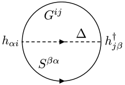
Figure 2: An example of 2PI diagrams for the Lagrangian (2.4) with Yukawa interactions. Each line represents a full propagator of the SM lepton, Higgs and the RH neutrino. By taking a functional derivative with respect to each propagator, we can obtain the self-energy for the corresponding particle.

The contribution to the lepton self-energy $\Sigma$ from Figure 2 is written in terms of the full propagators:

$$\Sigma^{\alpha\beta}_{ab\ \tiny\raisebox{-0.5pt}[0.0pt][0.0pt]{$\stackrel{{\scriptstyle\textstyle>}}{{\textstyle\rule{0.0pt}{1.5pt}\smash{<}}}$}}(x,y)= -\delta_{ab}h_{\alpha i}h^{{\dagger}}_{j\beta}P_{\rm R}G_{\tiny\raisebox{-0.5pt}[0.0pt][0.0pt]{$\stackrel{{\scriptstyle\textstyle>}}{{\textstyle\rule{0.0pt}{1.5pt}\smash{<}}}$}}^{ij}(x,y)P_{\rm L}\Delta_{\tiny\raisebox{-0.5pt}[0.0pt][0.0pt]{$\stackrel{{\scriptstyle\textstyle<}}{{\textstyle\rule{0.0pt}{1.5pt}\smash{>}}}$}}(y,x)\equiv\ \delta_{ab}\Sigma^{\alpha\beta}_{\tiny\raisebox{-0.5pt}[0.0pt][0.0pt]{$\stackrel{{\scriptstyle\textstyle>}}{{\textstyle\rule{0.0pt}{1.5pt}\smash{<}}}$}}(x,y)\ .$$ (2.46)

Recall that $(i,j)$ are flavor indices of the RH neutrinos. Then, summing the lepton flavor $\alpha,\beta$ and $SU(2)_{L}$ isospin $a,b$ indices, we have

$$\frac{dn_{L}}{dt}+3Hn_{L}=-g_{w}h_{\alpha i}h^{{\dagger}}_{j\beta}\int^{x^{0}}_{t_{int}}d^{4}z_{g}\ {\bigg{[}} {\rm tr}{\Big{\{}}P_{\rm R}G_{<}^{ij}(z,x)P_{\rm L}S^{\beta\alpha}_{>}(x,z){\Big{\}}}\Delta_{>}(x,z)$$

$$- {\rm tr}{\Big{\{}}P_{\rm R}G_{>}^{ij}(z,x)P_{\rm L}S^{\beta\alpha}_{<}(x,z){\Big{\}}}\Delta_{<}(x,z)$$

$$- {\rm tr}{\Big{\{}}P_{\rm R}G_{>}^{ij}(x,z)P_{\rm L}S^{\beta\alpha}_{<}(z,x){\Big{\}}}\Delta_{<}(z,x)$$

$$+ {\rm tr}{\Big{\{}}P_{\rm R}G_{<}^{ij}(x,z)P_{\rm L}S^{\beta\alpha}_{>}(z,x){\Big{\}}}\Delta_{>}(z,x){\bigg{]}}\ .$$ (2.47)

Here we used the fact that the electroweak symmetry is restored at the temperature $T\gtrsim{\rm TeV}$ we are in mind and hence the propagators are written in $SU(2)$ symmetric forms: $S^{\alpha\beta}_{ab}=S^{\alpha\beta}\delta_{ab}$, $\Delta_{ab}=\Delta\delta_{ab}$. $g_{w}=2$ is the number of d.o.f. of $SU(2)_{L}$ doublets. Since the third and the fourth terms are complex conjugate to the second and the first terms, we can simplify the above equation as

$$\frac{dn_{L}}{dt}+3Hn_{L}=2\ \Re\int^{x^{0}}_{t_{int}}d\tau d^{3}{\bf z}_{g}\ h_{\alpha i}h^{{\dagger}}_{j\beta}{\Big{[}} {\rm tr}{\Big{\{}}P_{\rm R}G_{<}^{ij}(x,z)P_{\rm L}\widetilde{\pi}_{>}^{\beta\alpha}(z,x){\Big{\}}}$$

$$- {\rm tr}{\Big{\{}}P_{\rm R}G_{>}^{ij}(x,z)P_{\rm L}\widetilde{\pi}_{<}^{\beta\alpha}(z,x){\Big{\}}}{\Big{]}}$$ (2.48)

where we have defined $\tau=z^{0}$ and

$$\widetilde{\pi}_{\gtrless}^{\beta\alpha}(z,x)=-g_{w}S^{\beta\alpha}_{\gtrless}(z,x)\Delta_{\gtrless}(z,x)\ .$$ (2.49)

This is the equation we evaluate in the following investigations. As we mentioned above, the r.h.s. contains only the contribution from the simplest 2PI diagram of Figure 2. This corresponds to taking the processes of decay and inverse-decay of the RH neutrinos. The effects of scattering can be taken into account by considering the next simplest diagram of Figure 5. A systematical study of the KB equation including the scattering effects is given in [68][69].

2.5 Boltzmann equation for the lepton number

The evolution equation (2.48) of the lepton number is determined by the behavior of full propagators of the RH neutrinos $G$, the SM leptons $S$ and the Higgs $\Delta$. In sections 3 and 4, we investigate detailed properties of the propagator $G$ of the RH neutrinos. In this section, we will see how an ordinary Boltzmann-type equation can be derived from eq.(2.48) by using the quasi-particle approximation for the SM particles described by $S$ and $\Delta.$

The quasi-particle approximation is an approximation to express the Green functions in terms of distribution functions of quasi-particles with a mass $m$ and a width $\Gamma$. Hence the propagators in this approximation are obtained from the free Wightman function of eq.(2.12) by introducing the decay width $\Gamma$. For a moment, we neglect the time-dependence of the background. For the SM leptons, we have

$$S^{\beta\alpha}_{\tiny\raisebox{-0.5pt}[0.0pt][0.0pt]{$\stackrel{{\scriptstyle\textstyle>}}{{\textstyle\rule{0.0pt}{1.5pt}\smash{<}}}$}}(x,y)=\ \delta^{\alpha\beta}\int\frac{d^{3}p}{(2\pi)^{3}}\frac{1}{2\omega_{p}}e^{+i{\mathbb{p}}\cdot({\mathbb{x}}-{\mathbb{y}})}\ e^{-|x^{0}-y^{0}|\Gamma_{\ell}/2}$$

$$\times {\Big{[}}e^{-i\omega_{p}(x^{0}-y^{0})}\left\{\begin{matrix}1-f_{\ell p}\\ -f_{\ell p}\end{matrix}\right\}P_{\rm L}{\ooalign{\hfil/\hfil\crcr$p$}}_{+}P_{\rm R}+e^{+i\omega_{p}(x^{0}-y^{0})}\left\{\begin{matrix}-f_{\overline{\ell}p}\\ 1-f_{\overline{\ell}p}\end{matrix}\right\}P_{\rm L}{\ooalign{\hfil/\hfil\crcr$p$}}_{-}P_{\rm R}{\Big{]}}$$ (2.54)

$$=\ \delta^{\alpha\beta}\sum_{\epsilon_{\ell}=\pm}\int\frac{d^{3}p}{(2\pi)^{3}}\frac{1}{2\omega_{p}}e^{+i{\mathbb{p}}\cdot({\mathbb{x}}-{\mathbb{y}})}e^{-i\epsilon_{\ell}\omega_{p}(x^{0}-y^{0})-|x^{0}-y^{0}|\Gamma_{\ell}/2}$$

$$\hskip 85.0pt\times(-1)^{\epsilon_{\ell}}\left\{\begin{matrix}1-f^{\epsilon_{\ell}}_{\ell p}\\ -f^{\epsilon_{\ell}}_{\ell p}\end{matrix}\right\}P_{\rm L}{\ooalign{\hfil/\hfil\crcr$p$}}_{\epsilon_{\ell}}P_{\rm R}$$ (2.57)

where $\omega_{p}=\sqrt{m_{\ell}^{2}+|{\mathbb{p}}|^{2}/a^{2}}$ and ${\ooalign{\hfil/\hfil\crcr$p$}}_{\pm}\equiv\pm\omega_{p}\gamma^{0}-{\mathbb{p}}\cdot{\boldsymbol{\gamma}}/a$. Here we assumed the flavor independence of the lepton propagators, $S^{\alpha\beta}\propto\delta^{\alpha\beta}$, for simplicity. Similarly the Wightman functions of the Higgs boson becomes

$$\Delta_{\tiny\raisebox{-0.5pt}[0.0pt][0.0pt]{$\stackrel{{\scriptstyle\textstyle>}}{{\textstyle\rule{0.0pt}{1.5pt}\smash{<}}}$}}(x,y)= \int\frac{d^{3}k}{(2\pi)^{3}}\frac{1}{2\omega_{k}}e^{+i{\mathbb{k}}\cdot({\mathbb{x}}-{\mathbb{y}})}e^{-|x^{0}-y^{0}|\Gamma_{\phi}/2}$$

$$\times{\Big{[}}e^{-i\omega_{k}(x^{0}-y^{0})}\left\{\begin{matrix}1+f_{\phi k}\\ +f_{\phi k}\end{matrix}\right\}+e^{+i\omega_{k}(x^{0}-y^{0})}\left\{\begin{matrix}+f_{\overline{\phi}k}\\ 1+f_{\overline{\phi}k}\end{matrix}\right\}{\Big{]}}$$

$$= \sum_{\epsilon_{\phi}=\pm}\int\frac{d^{3}k}{(2\pi)^{3}}\frac{1}{2\omega_{k}}e^{+i{\mathbb{k}}\cdot({\mathbb{x}}-{\mathbb{y}})}e^{-i\epsilon_{\phi}\omega_{k}(x^{0}-y^{0})-|x^{0}-y^{0}|\Gamma_{\phi}/2}$$

$$\hskip 70.0pt\times(-1)^{\epsilon_{\phi}}\left\{\begin{matrix}1+f^{\epsilon_{\phi}}_{\phi k}\\ +f^{\epsilon_{\phi}}_{\phi k}\end{matrix}\right\}\$$ (2.58)

where $\omega_{k}=\sqrt{m_{\phi}^{2}+|{\mathbb{k}}|^{2}/a^{2}}$ .

The thermal mass and width are given by $m_{\ell,\phi}\sim gT\ ,\ \Gamma_{\ell,\phi}\sim g^{2}T$ where $g$ is the SM gauge coupling $g$. The effects of the thermal plasma play very important roles, and are systematically investigated in [68][69]. For example, the thermal mass of the Higgs becomes larger than the RH neutrino masses at very high temperature. In the present paper, we focus on the largeness of $\Gamma_{\ell,\phi}$ as an important thermal effect and do not consider other effects.

In these expressions we defined $(-1)^{\epsilon}=\pm 1$ for $\epsilon=\pm$ respectively. The distribution functions are assumed to be in the kinematical equilibrium and given by the Fermi-Dirac or the Bose-Einstein distributions at temperature $T$ with a chemical potential:

$$f_{\ell p}=\frac{1}{e^{(\omega_{p}-\mu_{\ell})/T}+1}\ ,\ f_{\phi k}=\frac{1}{e^{(\omega_{k}-\mu_{\phi})/T}-1}\ .\$$ (2.59)

For anti-particles, the signs of the chemical potentials are reversed and their distributions are given by

$$f_{\overline{\ell}p}=\frac{1}{e^{(\omega_{p}+\mu_{\ell})/T}+1}\ ,\ \ f_{\overline{\phi}k}=\frac{1}{e^{(\omega_{k}+\mu_{\phi})/T}-1}\ .$$ (2.60)

In the second equalities of eq. (2.57) and (2.58), we have defined

$$f^{\epsilon}_{\ell p}\equiv\frac{1}{e^{(\epsilon\omega_{p}-\mu_{\ell})/T}+1}\ ,\ \ f^{\epsilon}_{\phi k}\equiv\frac{1}{e^{(\epsilon\omega_{k}-\mu_{\phi})/T}-1}$$ (2.61)

which satisfy

$$f_{\ell p}=f^{+}_{\ell p}\ ,\ \ f_{\overline{\ell}p}=(1-f^{-}_{\ell p})\ ,\ \ f_{\phi k}=f^{+}_{\phi k}\ ,\ \ f_{\overline{\phi}k}=-(1+f^{-}_{\phi k})\ .$$ (2.62)

Now we come back to the time-dependence of the background. Since the scale factor $a(t)$ is time-dependent, temperature $T$, thermal mass and width are dependent on the time $t$ and we need to specify at which time these quantities in the quasi-particle approximation of eq. (2.57) and (2.58) are defined. If the temperature of the universe is sufficiently low (e.g., $\sim$ 10 TeV), the decay width is much larger than the Hubble expansion rate:

$$\Gamma_{\ell,\phi}\sim g^{2}T\gg H\sim\frac{T^{2}}{10^{18}{\rm GeV}}$$ (2.63)

and the propagators damp quickly at $|x^{0}-y^{0}|\gg 1/\Gamma_{l,\phi}$. For such short period, time-dependence of the physical quantities such as the scale factor in the propagators (2.57) and (2.58) are suppressed by $H/\Gamma_{\ell,\phi}$, and we can approximate these quantities as being constant in the integration of $\tau$ in (2.48). Then the physical quantities can be evaluated at time $t=X_{xy}=(x^{0}+y^{0})/2$ as we see in (4.4).

By Fourier transforming in the spatial direction and using the above approximation, (2.48) becomes

$$\frac{dn_{L}}{dt}+3Hn_{L}=2\Re\int\frac{d^{3}q}{(2\pi)^{3}}\int^{t}_{-\infty}d\tau\ (h^{{\dagger}}h)_{ji}{\bigg{[}} {\rm tr}{\Big{\{}}P_{\rm R}G_{<}^{ij}(t,\tau;{\mathbb{q}})P_{\rm L}\widetilde{\pi}_{>}(\tau,t;{\mathbb{q}}){\Big{\}}}$$

$$- {\rm tr}{\Big{\{}}P_{\rm R}G_{>}^{ij}(t,\tau;{\mathbb{q}})P_{\rm L}\widetilde{\pi}_{<}(\tau,t;{\mathbb{q}}){\Big{\}}}{\bigg{]}}$$ (2.64)

where $t=x^{0}$ and $d^{3}q=d^{3}{\bf q}/a^{3}(t)$. Using the quasi-particle approximations (2.57) and (2.58), $\widetilde{\pi}_{\tiny\raisebox{-0.5pt}[0.0pt][0.0pt]{$\stackrel{{\scriptstyle\textstyle>}}{{\textstyle\rule{0.0pt}{1.5pt}\smash{<}}}$}}(\tau,t;{\bf q})$ are given by

$$\widetilde{\pi}_{\tiny\raisebox{-0.5pt}[0.0pt][0.0pt]{$\stackrel{{\scriptstyle\textstyle>}}{{\textstyle\rule{0.0pt}{1.5pt}\smash{<}}}$}}(\tau,t;{\bf q})=P_{\rm L}\pi_{\tiny\raisebox{-0.5pt}[0.0pt][0.0pt]{$\stackrel{{\scriptstyle\textstyle>}}{{\textstyle\rule{0.0pt}{1.5pt}\smash{<}}}$}}(\tau,t;{\bf q})P_{\rm R}\ ,$$ (2.65)

$$\pi_{\tiny\raisebox{-0.5pt}[0.0pt][0.0pt]{$\stackrel{{\scriptstyle\textstyle>}}{{\textstyle\rule{0.0pt}{1.5pt}\smash{<}}}$}}(\tau,t;{\bf q})\equiv(-g_{w})\sum_{\epsilon_{\ell},\epsilon_{\phi}} \int\frac{d^{3}p}{(2\pi)^{3}2\omega_{p}}\frac{d^{3}k}{(2\pi)^{3}2\omega_{k}}\ (2\pi)^{3}\delta^{3}(q-p-k)$$

$$\times\ {\mathcal{D}}_{\tiny\raisebox{-0.5pt}[0.0pt][0.0pt]{$\stackrel{{\scriptstyle\textstyle>}}{{\textstyle\rule{0.0pt}{1.5pt}\smash{<}}}$}(p,k)}^{\epsilon_{\ell}\epsilon_{\phi}}\ {\ooalign{\hfil/\hfil\crcr$p$}}_{\epsilon_{\ell}}\ e^{-i(\epsilon_{\ell}\omega_{p}+\epsilon_{\phi}\omega_{k})(\tau-t)-\Gamma_{\ell\phi}/2|\tau-t|}$$ (2.68)

where $\Gamma_{\ell\phi}\equiv\Gamma_{\ell}+\Gamma_{\phi}$ and ${\mathcal{D}}_{\tiny\raisebox{-0.5pt}[0.0pt][0.0pt]{$\stackrel{{\scriptstyle\textstyle>}}{{\textstyle\rule{0.0pt}{1.5pt}\smash{<}}}$}(p,k)}^{\epsilon_{\ell}\epsilon_{\phi}}$ is defined as

$${\mathcal{D}}_{\tiny\raisebox{-0.5pt}[0.0pt][0.0pt]{$\stackrel{{\scriptstyle\textstyle>}}{{\textstyle\rule{0.0pt}{1.5pt}\smash{<}}}$}(p,k)}^{\epsilon_{\ell}\epsilon_{\phi}}\equiv(-1)^{\epsilon_{\ell}}(-1)^{\epsilon_{\phi}}\left\{\begin{matrix}(1-f_{\ell p}^{\epsilon_{\ell}})(1+f_{\phi k}^{\epsilon_{\phi}})\\ (-f_{\ell p}^{\epsilon_{\ell}})(+f_{\phi k}^{\epsilon_{\phi}})\end{matrix}\right\}\ .$$ (2.69)

From (2.68) and (2.69), we can see that the term with $\widetilde{\pi}_{>}$ in (2.64) contains a factor $(1-f_{\ell})$ or $(1-f_{\ell}^{-})=f_{\bar{\ell}}$ and corresponds to gain in the lepton number while the other term with $\widetilde{\pi}_{<}$ contains a factor $f_{\ell}$ or $f_{\ell}^{-}=(1-f_{\bar{\ell}})$ and corresponds to loss. Hence the evolution equation (2.64) can be interpreted as the Boltzmann-like equation for the lepton number.

In order to solve the evolution equation (2.64), we need detailed information of the Wightman function $G_{\gtrless}^{ij}(x,y)$ of the RH neutrinos. In the following sections, we obtain behaviors of the Wightman Green functions, especially deviations from the thermal equilibrium values in the expanding universe.

Here we briefly comment on the basic structures of the r.h.s. First, contributions from the flavor diagonal part $i=j$ are evaluated by the quasi-particle approximation. $G_{\lessgtr}^{ii}$ is proportional to $(f_{N_{i}}^{\epsilon})$ or $(1-f_{N_{i}}^{\epsilon})$ respectively where $f_{N_{i}}$ is the distribution function of the RH neutrino $N_{i}$. Therefore, combined with the distribution functions from $\widetilde{\pi}_{\gtrless}$, flavor diagonal term gives the tree-level decay or inverse-decay of Figure 1, and wash out the generated lepton number asymmetry.

On the other hand, by using the formal solution of the Wightman function in (2.16), contributions from the flavor off-diagonal part $i\neq j$ are interpreted as an interference effect between the tree and 1-loop diagrams as follows. The formal solution is written in terms of the self-energy $\Pi_{\gtrless}$ as

$$G_{\tiny\raisebox{-0.5pt}[0.0pt][0.0pt]{$\stackrel{{\scriptstyle\textstyle>}}{{\textstyle\rule{0.0pt}{1.5pt}\smash{<}}}$}}^{ij}(x,y)= -\sum_{k,l}\int_{-\infty}^{x^{0}}du^{0}d^{3}{\bf u}_{g}\int_{-\infty}^{y^{0}}dv^{0}d^{3}{\bf v}_{g}\ G_{R}^{ik}(x,u)\Pi_{\tiny\raisebox{-0.5pt}[0.0pt][0.0pt]{$\stackrel{{\scriptstyle\textstyle>}}{{\textstyle\rule{0.0pt}{1.5pt}\smash{<}}}$}}^{kl}(u,v)G^{lj}_{A}(v,y)\ .$$ (2.70)

In the leading order approximation with the 2PI diagram of Figure 2, the self-energy $\Pi_{\gtrless}$ is written as a functional of the full propagators of the SM lepton and the Higgs as in eq.(D.6). Hence it can be interpreted as an interaction vertex of $\ell\phi\leftrightarrow N$ at $u\sim v$. The RH neutrino propagates from $u\sim v$ to another interaction vertex at $x\sim y$. By inserting this expression into eq.(2.64) and taking the on-shell limit of the RH neutrinos, $CP$-asymmetric interference between the tree and the one-loop self-energy diagram can be obtained. If the RH neutrinos propagating between these vertices are off-shell, the contribution is interpreted as s-channel scattering processes. Hence flavor off-diagonal terms in the r.h.s. of (2.64) give both of the $CP$-asymmetric decay of the RH neutrinos and the washout of the lepton numbers via s-channel scattering of leptons and Higgs.

In the resonant leptogenesis where the RH neutrinos have almost degenerate masses, however, it is not legitimate to separate the on-shell and off-shell contributions as above since the RH neutrinos are coherently mixed between different flavors, as has been mentioned in [61][68]. Therefore we need to scrutinize the behavior of the Wightman functions $G_{\gtrless}^{ij}(t,\tau;{\bf q})$ in the expanding universe.

2.6 Summary of this section

The evolution of the lepton number is given by (2.48) or its Fourier transform (2.64). They are the basic equations we evaluate in the following sections. If we adopt the quasi-particle approximations of (2.57) or (2.58), an ordinary classical Boltzmann equation is derived. But in the resonant leptogenesis, quantum coherence between different flavors of $N_{i}$ plays an essential role and such an approximation is not valid for the RH neutrinos. An evaluation of the r.h.s. of (2.48) by scrutinizing the behavior of the off-diagonal components of the Wightman functions $G_{\gtrless}^{ij}$, which is formally solved as (2.70), in the expanding universe is the main issue in the following sections.

3 Resonant oscillation of RH neutrinos

In this section, we study how the RH neutrinos with almost degenerate masses behave in the thermal equilibrium. Deviation from the thermal equilibrium is investigated in the next section 4.

We consider two flavors $i=1,2$ whose masses are almost degenerate. The third flavor RH neutrino is assumed to have larger mass. In order to calculate the evolution of the lepton asymmetry in (2.48), we need to know the Wightman functions $G_{\gtrless}$ of the RH neutrinos. And, since the KB equation of $G_{\gtrless}^{ij}$ is formally solved by the convolution eq.(2.70), it is necessary to investigate the properties of the retarded (advanced) Green functions $G_{R/A}^{ij}$ first.

We first study both of the flavor diagonal ($i=j$) and off-diagonal ($i\neq j$) components of $G_{R}^{ij}$ in the equilibrium. Then we will see the behaviors of the Wightman functions $G_{\gtrless}^{ij}$ in the thermal equilibrium. Throughout the paper, $G^{d}$ (also $\Pi^{d}$ for the self-energy) and $G^{\prime}$ ($\Pi^{\prime}$) denote the flavor diagonal $i=j$ and off-diagonal $i\neq j$ components respectively:

$$G^{d} \longleftrightarrow\ \ \mbox{flavor diagonal },$$ (3.1)

$$G^{\prime} \longleftrightarrow\ \ \mbox{flavor off-diagonal }.$$

3.1 Retarded/Advanced propagators

From (2.13) and (2.24), $G_{R/A}$ satisfies

$$(i{\ooalign{\hfil/\hfil\crcr$\nabla$}}_{x}-M)G^{ij}_{R/A}(x,y)-\int^{\infty}_{t_{int}}dz^{0}d^{3}{\bf z}\ a^{3}(z^{0})\ \Pi^{ik}_{R/A}(x,z)G^{kj}_{R/A}(z,y) =-\delta_{ij}\delta^{g}(x-y)\ .$$ (3.4)

We first define the spatial Fourier transform of $G_{R/A}$ by

$$G^{ij}_{R/A}(x^{0},y^{0};{\mathbb{q}})=\int d^{3}({\mathbb{x}}-{\mathbb{y}})e^{-i{\mathbb{q}}\cdot({\mathbb{x}}-{\mathbb{y}})}a^{3/2}(x^{0})G^{ij}_{R/A}(x^{0},y^{0},{\mathbb{x}}-{\mathbb{y}})a^{3/2}(y^{0})\ .$$ (3.5)

Similarly, for the self-energy, we define

$$\Pi^{ij}_{R/A}(x^{0},y^{0};{\mathbb{q}})=\int d^{3}({\mathbb{x}}-{\mathbb{y}})e^{-i{\mathbb{q}}\cdot({\mathbb{x}}-{\mathbb{y}})}a^{3/2}(x^{0})\Pi^{ij}_{R/A}(x^{0},y^{0},{\mathbb{x}}-{\mathbb{y}})a^{3/2}(y^{0})\ .$$ (3.6)

Then using (2.33), the KB equation (3.4) becomes

$${\Big{\{}}i\gamma^{0} \partial_{x^{0}}-\frac{{\boldsymbol{\gamma}}\cdot{\mathbb{q}}}{a(x^{0})}-M{\Big{\}}}G_{R/A}(x^{0},y^{0};{\mathbb{q}})$$

$$-\int^{\infty}_{t_{int}}dz^{0}\ \Pi_{R/A}(x^{0},z^{0};{\mathbb{q}})G_{R/A}(z^{0},y^{0};{\mathbb{q}})=-\delta(x^{0}-y^{0})\ .$$ (3.7)

This is the basic equation for $G_{R/A}$.

We then decompose the propagator and the self-energy into flavor diagonal and off-diagonal parts:

$$G_{R/A}(x^{0},y^{0};{\mathbb{q}}) \equiv G^{d}_{R/A}(x^{0},y^{0};{\mathbb{q}})+G^{\prime}_{R/A}(x^{0},y^{0};{\mathbb{q}})\ ,$$

$$\Pi_{R/A}(x^{0},y^{0};{\mathbb{q}}) \equiv\Pi^{d}_{R/A}(x^{0},y^{0};{\mathbb{q}})+\Pi^{\prime}_{R/A}(x^{0},y^{0};{\mathbb{q}})\ .$$ (3.8)

Using this decomposition, we solve the KB equation (3.7) iteratively.

First we define the differential-integral operator $D^{d}_{x^{0}}$ by

$$D^{d}_{x^{0}}f(x^{0})\equiv{\Big{\{}}i\gamma^{0}\partial_{x^{0}}-\frac{{\boldsymbol{\gamma}}\cdot{\mathbb{q}}}{a(x^{0})}-M{\Big{\}}}f(x^{0})-\int^{\infty}_{t_{int}}dz^{0}\ \Pi^{d}_{R/A}(x^{0},z^{0};{\mathbb{q}})\ f(z^{0})\ .$$ (3.9)

In terms of the operator, the flavor diagonal component of the KB equation (3.7) becomes

$$D^{d}_{x^{0}}G^{d}_{R/A}(x^{0},y^{0};{\mathbb{q}})-\int^{\infty}_{t_{int}}dz^{0}\ \Pi^{\prime}_{R/A}(x^{0},z^{0};{\mathbb{q}})G^{\prime}_{R/A}(z^{0},y^{0};{\mathbb{q}})=-\delta(x^{0}-y^{0})\ .$$ (3.10)

Similarly the KB equation of the flavor off-diagonal component is written as

$$D^{d}_{x^{0}}G^{\prime}_{R/A}(x^{0},y^{0};{\mathbb{q}})=\int^{\infty}_{t_{int}}dz^{0}\ \Pi^{\prime}_{R/A}(x^{0},z^{0};{\mathbb{q}})G^{d}_{R/A}(z^{0},y^{0};{\mathbb{q}})\ .$$ (3.11)

We then introduce the kernel $G_{R/A}^{d(0)}$ of the operator $D_{x^{0}}^{d}$:

$$D^{d}_{x^{0}}G^{d(0)}_{R/A}(x^{0},y^{0};{\mathbb{q}})\equiv-\delta(x^{0}-y^{0})\ .$$ (3.12)

with a retarded (advanced) boundary condition. Using $G_{R/A}^{d(0)}$, we can integrate the equations (3.10), (3.11) as

$$G^{d}_{R/A}(x^{0},y^{0};{\mathbb{q}}) =G^{d(0)}_{R/A}(x^{0},y^{0};{\mathbb{q}})$$

$$-\int^{\infty}_{t_{int}}d\tau d\tau^{\prime}\ G^{d(0)}_{R/A}(x^{0},\tau;{\mathbb{q}})\Pi^{{}^{\prime}}_{R/A}(\tau,\tau^{\prime};{\mathbb{q}})G^{\prime}_{R/A}(\tau,y^{0};{\mathbb{q}})\ ,$$ (3.13)

$$G^{\prime}_{R/A}(x^{0},y^{0};{\mathbb{q}})=-\int^{\infty}_{t_{int}}d\tau d\tau^{\prime}\ G^{d(0)}_{R/A}(x^{0},\tau;{\mathbb{q}})\Pi^{{}^{\prime}}_{R/A}(\tau,\tau^{\prime};{\mathbb{q}})G^{d}_{R/A}(\tau,y^{0};{\mathbb{q}})\ .$$ (3.14)

Then we can iteratively solve the above equations by expanding it with respect to the small off-diagonal component of the Yukawa coupling $(h^{{\dagger}}h)^{{}^{\prime}}$ involved in $\Pi^{{}^{\prime}}$:

$$G^{d}_{R/A}= G^{d(0)}_{R/A}+G^{d(2)}_{R/A}+\cdots,$$ (3.15)

$$G^{d(2)}_{R/A}\equiv G^{d(0)}_{R/A}*\Pi^{{}^{\prime}}_{R/A}*G^{d(0)}_{R/A}*\Pi^{{}^{\prime}}_{R/A}*G^{d(0)}_{R/A}\ ,$$

$$G^{\prime}_{R/A}= -G^{d(0)}_{R/A}*\Pi^{{}^{\prime}}_{R/A}*G^{d(0)}_{R/A}+\cdots\ .$$ (3.16)

Here $*$ denotes a convolution in the time-direction. The second term $G^{d(2)}_{R/A}$ in the flavor diagonal propagator (3.15) is the second order of $(h^{{\dagger}}h)^{{}^{\prime}}$ and smaller than $G^{d(0)}_{R/A}$ or $G^{\prime}_{R/A}$. Hence we drop it and write $G^{d(0)}$ as $G^{d}$ for notational simplicity in the following.

We note that the above integrals do not have the memory effect. This is because the convolution is written explicitly as, e.g.,

$$(G_{R}*\Pi_{R}*G_{R})(x^{0},y^{0})=\int^{x^{0}}_{y^{0}}du\int_{y^{0}}^{u}\ dv\ G_{R}(x^{0},u)\Pi_{R}(u,v)G_{R}(v,y^{0})$$ (3.17)

and the integration region is limited between $x^{0}$ and $y^{0}$. Namely, the retarded (advanced) propagators are ”local” functions of time during $x^{0}$ and $y^{0}$ and insensitive to the past ($t<x^{0},y^{0}$). This is different from the convolution contained in the Wightman functions (2.70) in which the integration range of time is extended to the past.

3.2 Diagonal $G_{R/A}^{d}$ in thermal equilibrium

We will first look at the flavor diagonal component of the propagator $G^{d}_{R/A}(x^{0},y^{0};{\bf q})$ in the thermal equilibrium at temperature $T$. The scale factor $a$ is also fixed at $a_{0}=a(x^{0})=a(y^{0}).$ Because of the translational invariance in the time direction, $G_{R/A}(x^{0},y^{0};{\bf q})$ can be further Fourier transformed:

$$G^{d(eq)}_{R/A}(q)=\int d(x^{0}-y^{0})e^{+iq_{0}(x^{0}-y^{0})}G^{d(eq)}_{R/A}(x^{0},y^{0};{\mathbb{q}})\ .$$ (3.18)

Then the KB equation (3.13) becomes

$${\Big{\{}}\gamma^{0}q_{0}-\frac{{\boldsymbol{\gamma}}\cdot{\mathbb{q}}}{a_{0}}-M-\Pi^{d(eq)}_{R/A}(q_{0},{\mathbb{q}}){\Big{\}}}G^{d(eq)}_{R/A}(q)=-1\$$ (3.19)

and can be solved

$$G^{d(eq)}_{R/A}(q) =-\left({\ooalign{\hfil/\hfil\crcr$q$}}-M-\Pi^{d(eq)}_{R/A}(q)\right)^{-1}.$$ (3.22)

The real part of the self-energy gives the mass and wave-function renormalization. In the following we assume that they are already taken into account in the bare Lagrangian and focus only on the imaginary part $\Pi^{d}_{\rho}=\Pi^{d}_{R}-\Pi^{d}_{A}=2i\Im(\Pi^{d}_{R})$. The one-loop diagonal self-energy in the thermal equilibrium is expressed as $\Pi_{\rho}^{d}=\gamma^{\mu}\Pi_{\rho,\mu}^{d}$. From the imaginary part of the pole of the propagator $G_{R}^{d(eq)}(q)$, we see that the decay width $\Gamma_{q}$ of the RH neutrino is given by

$$q\cdot\Pi^{d(eq)}_{\rho}(q)|_{q_{0}=\pm\omega_{\mathbb{q}}}\equiv\mp i\omega_{q}\Gamma_{q}\ .$$ (3.23)

The $i$-th diagonal component $G^{d(eq)ii}_{R/A}(q)$ becomes

$$G^{d(eq)ii}_{R/A}(q) \simeq-\frac{{\ooalign{\hfil/\hfil\crcr$q$}}-\Pi^{d(eq)ii}_{R/A}(q)+M_{i}}{(q_{0}\pm i\Gamma_{iq}/2)^{2}-\omega_{iq}^{2}}\simeq\left\{\begin{matrix}\displaystyle\sum_{\epsilon=\pm}\frac{iZ_{\epsilon}^{i}}{q_{0}-\Omega_{\epsilon i}}\\ \displaystyle\sum_{\epsilon=\pm}\frac{iZ_{\epsilon}^{i}}{q_{0}-\Omega^{*}_{\epsilon i}}\end{matrix}\right.$$ (3.26)

where

$$\Omega_{\epsilon i}\equiv\epsilon\omega_{iq}-i\Gamma_{iq}/2$$ (3.27)

and

$$Z_{\epsilon}^{i}=\frac{i\epsilon}{2\omega_{iq}}({\ooalign{\hfil/\hfil\crcr$q$}}_{\epsilon i}+M_{i}),\ \ {\ooalign{\hfil/\hfil\crcr$q$}}_{\epsilon i}\equiv\epsilon\omega_{iq}\gamma^{0}-{\mathbb{q}}\cdot{\boldsymbol{\gamma}}/a_{0}\ .$$ (3.32)

In the real time representation, it becomes

$$G_{R}^{d(eq)ii}(x^{0},y^{0};{\mathbb{q}})=+\Theta(x^{0}-y^{0})\sum_{\epsilon=\pm}Z_{\epsilon}^{i}e^{-i\Omega_{\epsilon i}(x^{0}-y^{0})}\ ,$$

$$G_{A}^{d(eq)ii}(x^{0},y^{0};{\mathbb{q}})=-\Theta(y^{0}-x^{0})\sum_{\epsilon=\pm}Z_{\epsilon}^{i}e^{-i\Omega^{*}_{\epsilon i}(x^{0}-y^{0})}\ .$$ (3.33)

$\Gamma_{q}$ is multiplied by the Lorentz boost factor as $\Gamma_{q}\simeq(M/\omega_{q})\times\Gamma$ where $\Gamma\equiv\Gamma_{q=0}$ is the decay width of the RH neutrino. In the present paper, we consider a situation that two RH neutrinos are almost degenerate in their masses

$$\Delta M\equiv|M_{i}-M_{j}|\simeq\Gamma\ .$$ (3.34)

In the following, we sometimes use the averages denoted by quantities without the flavor index $i,j$

$$M=\frac{M_{i}+M_{j}}{2}\ ,\ \ \omega_{q}=\frac{\omega_{iq}+\omega_{jq}}{2}\ ,\ \ \Omega_{\epsilon}=\frac{\Omega_{\epsilon i}+\Omega_{\epsilon j}}{2}\ ,\ \ etc.$$ (3.35)

3.3 Off-diagonal $G_{R/A}^{\prime}$ in thermal equilibrium

We then study the behavior of the flavor off-diagonal component $G^{{}^{\prime}(eq)}_{R/A}$ of the retarded (advanced) propagators in the thermal equilibrium. From (3.16), it is given by

$$G_{R/A}^{{}^{\prime}(eq)ij}(x^{0},y^{0};{\mathbb{q}})=-\int\frac{dq_{0}}{2\pi}e^{-iq_{0}(x^{0}-y^{0})}G_{R/A}^{d(eq)ii}(q)\Pi^{{}^{\prime}(eq)ij}_{R/A}(q)G_{R/A}^{d(eq)jj}(q)\ .$$ (3.36)

The $q_{0}$ integration can be performed by summing residues of the poles. Eq. (3.26) shows that the retarded propagator $G_{R}^{d(eq)ii}$ has poles at $q_{0}=\Omega_{\pm,i}$ and the advanced propagator $G_{A}^{d(eq)jj}$ has poles at $q_{0}=\Omega_{\pm,j}^{*}$. The self-energy $\Pi_{R/A}$ consists of the SM lepton and the Higgs propagator, and hence it has poles at $q_{0}=\epsilon_{\ell}\omega_{p}+\epsilon_{\phi}\omega_{k}\mp i\Gamma_{\ell\phi}/2$ with a large imaginary part. Because of this, the residues of the poles of the self-energy are suppressed by $\Gamma_{i}/\Gamma_{\ell\phi}\ll 1$. Noting the relation

$$\frac{1}{q_{0}-\Omega_{\epsilon i}}\frac{1}{q_{0}-\Omega_{\epsilon^{\prime}j}}=\frac{1}{\Omega_{\epsilon i}-\Omega_{\epsilon^{\prime}j}}\left(\frac{1}{q_{0}-\Omega_{\epsilon i}}-\frac{1}{q_{0}-\Omega_{\epsilon^{\prime}j}}\right)\ ,$$ (3.37)

we can see that the contribution $\epsilon=-\epsilon^{\prime}$ is also suppressed by $\Delta M/M$ compared to the $\epsilon=\epsilon^{\prime}$ contribution. Hence, dropping these suppressed contributions, we have

$$G_{R}^{{}^{\prime}(eq)ij}(x^{0},y^{0};{\mathbb{q}})\simeq +\Theta(x^{0}-y^{0})\sum_{\epsilon}Z_{\epsilon}\Pi^{{}^{\prime}(eq)ij}_{R}(\epsilon\omega_{q})Z_{\epsilon}\frac{-i}{\Omega_{\epsilon i}-\Omega_{\epsilon j}}$$

$$\hskip 40.0pt\times\left(e^{-i\Omega_{\epsilon i}(x^{0}-y^{0})}-e^{-i\Omega_{\epsilon j}(x^{0}-y^{0})}\right)\$$ (3.38)

and

$$G_{A}^{{}^{\prime}(eq)ij}(x^{0},y^{0};{\mathbb{q}})\simeq -\Theta(y^{0}-x^{0})\sum_{\epsilon}Z_{\epsilon}\Pi^{{}^{\prime}(eq)ij}_{A}(\epsilon\omega_{q})Z_{\epsilon}\frac{-i}{\Omega^{*}_{\epsilon i}-\Omega^{*}_{\epsilon j}}$$

$$\hskip 40.0pt\times\left(e^{-i\Omega^{*}_{\epsilon i}(x^{0}-y^{0})}-e^{-i\Omega^{*}_{\epsilon j}(x^{0}-y^{0})}\right)\ .$$ (3.39)

We also used the approximation $\Pi(\Omega_{\epsilon i})\simeq\Pi(\Omega_{\epsilon j})\simeq\Pi(\epsilon\omega_{q})$ because $\Gamma_{i}\ll\Gamma_{\ell\phi}$.

The minus signs in the parentheses come from the relative minus sign of the residue in (3.37). Because of this, the off-diagonal Green functions vanish at $x^{0}=y^{0}$:

$$G_{R/A}^{\prime}(x,y){\big{|}}_{x^{0}=y^{0}}=0\ .$$ (3.40)

This should generally hold by the definition of $G_{R/A}$ in (2.10) because $G_{\rho}^{ij}(x,y)$ is proportional to $\delta^{ij}\delta^{3}({\bf x}-{\bf y})$ at equal time $x^{0}=y^{0}$:

$$\gamma^{0}G^{ij}_{R}(x,y){\big{|}}_{x^{0}=y^{0}}=\Theta(x^{0}-y^{0})\gamma^{0}G^{ij}_{\rho}(x,y){\big{|}}_{x^{0}=y^{0}}=\frac{i}{2}\delta({\bf x}-{\bf y})\delta^{ij}\ .$$ (3.41)

Note that the flavor off-diagonal components of the retarded (advanced) propagators are enhanced by the factor $1/(\Omega_{i}-\Omega_{j})$ (or its complex conjugate). Such a large enhancement comes from the large mixing of the RH neutrinos with almost degenerate masses.

For the self-energies $\Pi_{R/A}=\Pi_{h}\pm\Pi_{\rho}/2$, if we use the vacuum value $\Pi^{\prime}_{\rho}(\epsilon\omega_{q})=-g_{w}\Re(h^{{\dagger}}h)^{\prime}i\epsilon{\ooalign{\hfil/\hfil\crcr$q$}}_{\epsilon}/(16\pi)$ and $\Pi^{\prime}_{h}(\epsilon\omega_{q})=0$ as in Appendix D, the following expressions [56] are reproduced:

$$G_{R}^{{}^{\prime}(eq)ij}(x^{0},y^{0};{\mathbb{q}})\simeq +\Theta(x^{0}-y^{0})\sum_{\epsilon}\frac{{\ooalign{\hfil/\hfil\crcr$q$}}_{\epsilon}+M}{2\omega_{q}}\frac{g_{w}M^{2}\Re(h^{{\dagger}}h)^{\prime}/(16\pi)}{M_{i}^{2}-M_{j}^{2}-i\epsilon(M_{i}\Gamma_{i}-M_{j}\Gamma_{j})}$$ (3.44)

$$\hskip 40.0pt\times\left(e^{-i\Omega_{\epsilon i}(x^{0}-y^{0})}-e^{-i\Omega_{\epsilon j}(x^{0}-y^{0})}\right)\ ,$$

$$G_{A}^{{}^{\prime}(eq)ij}(x^{0},y^{0};{\mathbb{q}})\simeq -\Theta(y^{0}-x^{0})\sum_{\epsilon}\frac{{\ooalign{\hfil/\hfil\crcr$q$}}_{\epsilon}+M}{2\omega_{q}}\frac{-g_{w}M^{2}\Re(h^{{\dagger}}h)^{\prime}/(16\pi)}{M_{i}^{2}-M_{j}^{2}+i\epsilon(M_{i}\Gamma_{i}-M_{j}\Gamma_{j})}$$ (3.47)

$$\hskip 40.0pt\times\left(e^{-i\Omega^{*}_{\epsilon i}(x^{0}-y^{0})}-e^{-i\Omega^{*}_{\epsilon j}(x^{0}-y^{0})}\right)\ .$$ (3.48)

Here we have used the relation

$$\frac{\epsilon}{2\omega_{q}}\frac{1}{\Omega_{\epsilon i}-\Omega_{\epsilon j}} \simeq\frac{1}{\omega_{iq}^{2}-\omega_{jq}^{2}-i\epsilon(\omega_{iq}\Gamma_{iq}-\omega_{jq}\Gamma_{jq})}$$

$$\simeq\frac{1}{M_{i}^{2}-M_{j}^{2}-i\epsilon(M_{i}\Gamma_{i}-M_{j}\Gamma_{j})}\$$ (3.49)

which is valid for $\omega_{q}\simeq\omega_{iq}\simeq\omega_{jq}$ and $\omega_{q}\Gamma_{q}\simeq M\Gamma$. Hence, the enhancement factor $1/(\Omega_{i}-\Omega_{j})$ corresponds to taking the regulator $(M_{i}\Gamma_{i}-M_{j}\Gamma_{j})$ is obtained. As shown in section 3.6, the same enhancement factor, that is, the same regulator appears in the off-diagonal Wightman function in the thermal equilibrium. For the deviations of the off-diagonal Wightman functions out of equilibrium, however, we show in section 4.5 that the enhancement factor is changed to be $1/(\Omega_{i}-\Omega_{j}^{*})$. This corresponds to the regulator $(M_{i}\Gamma_{i}+M_{j}\Gamma_{j}).$

Finally we note the validity of the expansion with respect to the off-diagonal components of the Yukawa couplings $(h^{{\dagger}}h)^{\prime}$. From the expressions (3.48), the iterative expansions (3.15) and (3.16) turn out to be valid when the real part of the off-diagonal components of Yukawa coupling $\Re(h^{{\dagger}}h)^{\prime}$ is smaller than the mass difference $|M_{i}-M_{j}|/M\simeq\Gamma/M\sim(h^{{\dagger}}h)^{d}_{ii}$. Hence the expansion is understood as an expansion of the ratio $(h^{\dagger}h)^{\prime}/(h^{\dagger}h)^{d}.$

3.4 Wightman functions

The Wightman functions can be solved as (2.16) or (2.70). If we take terms up to the first order of $(h^{{\dagger}}h)^{{}^{\prime}}$, the flavor diagonal component is given by

$$G^{dii}_{\tiny\raisebox{-0.5pt}[0.0pt][0.0pt]{$\stackrel{{\scriptstyle\textstyle>}}{{\textstyle\rule{0.0pt}{1.5pt}\smash{<}}}$}}= -G^{dii}_{R}*\Pi^{dii}_{\tiny\raisebox{-0.5pt}[0.0pt][0.0pt]{$\stackrel{{\scriptstyle\textstyle>}}{{\textstyle\rule{0.0pt}{1.5pt}\smash{<}}}$}}*G^{dii}_{A}\ .$$ (3.50)

Similarly the flavor off-diagonal component is given by

$$G^{{}^{\prime}ij}_{\tiny\raisebox{-0.5pt}[0.0pt][0.0pt]{$\stackrel{{\scriptstyle\textstyle>}}{{\textstyle\rule{0.0pt}{1.5pt}\smash{<}}}$}}= -G^{{}^{\prime}ij}_{R}*\Pi^{djj}_{\tiny\raisebox{-0.5pt}[0.0pt][0.0pt]{$\stackrel{{\scriptstyle\textstyle>}}{{\textstyle\rule{0.0pt}{1.5pt}\smash{<}}}$}}*G^{djj}_{A}-G^{dii}_{R}*\Pi^{dii}_{\tiny\raisebox{-0.5pt}[0.0pt][0.0pt]{$\stackrel{{\scriptstyle\textstyle>}}{{\textstyle\rule{0.0pt}{1.5pt}\smash{<}}}$}}*G^{{}^{\prime}ij}_{A}-G^{dii}_{R}*\Pi^{{}^{\prime}ij}_{\tiny\raisebox{-0.5pt}[0.0pt][0.0pt]{$\stackrel{{\scriptstyle\textstyle>}}{{\textstyle\rule{0.0pt}{1.5pt}\smash{<}}}$}}*G^{djj}_{A}\ .$$ (3.51)

By using (3.16) and (3.50), (3.51) can be also rewritten as

$$G^{{}^{\prime}ij}_{\tiny\raisebox{-0.5pt}[0.0pt][0.0pt]{$\stackrel{{\scriptstyle\textstyle>}}{{\textstyle\rule{0.0pt}{1.5pt}\smash{<}}}$}}= -G^{dii}_{R}*\Pi^{{}^{\prime}ij}_{R}*G^{djj}_{\tiny\raisebox{-0.5pt}[0.0pt][0.0pt]{$\stackrel{{\scriptstyle\textstyle>}}{{\textstyle\rule{0.0pt}{1.5pt}\smash{<}}}$}}-G^{dii}_{\tiny\raisebox{-0.5pt}[0.0pt][0.0pt]{$\stackrel{{\scriptstyle\textstyle>}}{{\textstyle\rule{0.0pt}{1.5pt}\smash{<}}}$}}*\Pi^{{}^{\prime}ij}_{A}*G^{djj}_{A}-G^{dii}_{R}*\Pi^{{}^{\prime}ij}_{\tiny\raisebox{-0.5pt}[0.0pt][0.0pt]{$\stackrel{{\scriptstyle\textstyle>}}{{\textstyle\rule{0.0pt}{1.5pt}\smash{<}}}$}}*G^{djj}_{A}$$ (3.52)

which makes it clear that the off-diagonal part of the self-energy causes the flavor mixing of the RH neutrino.

3.5 Diagonal Wightman $G_{\gtrless}^{d}$ in thermal equilibrium

In the thermal equilibrium, the Wightman function can be easily obtained by using the KMS relation. From (3.50), the diagonal component $G^{d(eq)}_{\tiny\raisebox{-0.5pt}[0.0pt][0.0pt]{$\stackrel{{\scriptstyle\textstyle>}}{{\textstyle\rule{0.0pt}{1.5pt}\smash{<}}}$}}$ can be written as

$$G_{\tiny\raisebox{-0.5pt}[0.0pt][0.0pt]{$\stackrel{{\scriptstyle\textstyle>}}{{\textstyle\rule{0.0pt}{1.5pt}\smash{<}}}$}}^{d(eq)}(x^{0},y^{0};{\mathbb{q}})= -\int\frac{dq_{0}}{2\pi}e^{-iq_{0}(x^{0}-y^{0})}G_{R}^{d(eq)}(q)\Pi^{d(eq)}_{\tiny\raisebox{-0.5pt}[0.0pt][0.0pt]{$\stackrel{{\scriptstyle\textstyle>}}{{\textstyle\rule{0.0pt}{1.5pt}\smash{<}}}$}}(q)G_{A}^{d(eq)}(q)\ .$$ (3.53)

Let $f(q)$ be the thermal distribution function for the RH neutrinos. Note that $f(q)$ is a function of $q^{0}$, which is not equal to the on-shell energy $\omega_{\bf q}.$ The KMS relation for the self-energy function is

$$\Pi^{(eq)}_{\tiny\raisebox{-0.5pt}[0.0pt][0.0pt]{$\stackrel{{\scriptstyle\textstyle>}}{{\textstyle\rule{0.0pt}{1.5pt}\smash{<}}}$}}(q)=-i\left\{\begin{matrix}1-f(q_{0})\\ -f(q_{0})\end{matrix}\right\}\Pi^{(eq)}_{\rho}(q)\ .$$ (3.54)

Using the solution of the KB equation for the spectral density $G_{\rho}\equiv G_{R}-G_{A}=-G_{R}*\Pi_{\rho}*G_{A}$, we have

$$G_{\tiny\raisebox{-0.5pt}[0.0pt][0.0pt]{$\stackrel{{\scriptstyle\textstyle>}}{{\textstyle\rule{0.0pt}{1.5pt}\smash{<}}}$}}^{d(eq)}(x^{0},y^{0};{\mathbb{q}})$$

$$=-\int\frac{dq_{0}}{2\pi}e^{-iq_{0}(x^{0}-y^{0})}(-i)\left\{\begin{matrix}1-f(q_{0})\\ -f(q_{0})\end{matrix}\right\}G_{R}^{d(eq)}(q)\Pi^{d(eq)}_{\rho}(q)G_{A}^{d(eq)}(q)$$

$$=+\int\frac{dq_{0}}{2\pi}e^{-iq_{0}(x^{0}-y^{0})}(-i)\left\{\begin{matrix}1-f(q_{0})\\ -f(q_{0})\end{matrix}\right\}\left[G_{R}^{d(eq)}(q)-G_{A}^{d(eq)}(q)\right]\ .$$ (3.55)

It is nothing but the KMS relation (2.11) for the Green function.

Performing the $q_{0}$ integration, it becomes

$$G_{\tiny\raisebox{-0.5pt}[0.0pt][0.0pt]{$\stackrel{{\scriptstyle\textstyle>}}{{\textstyle\rule{0.0pt}{1.5pt}\smash{<}}}$}}^{d(eq)ii}(x^{0},y^{0};{\mathbb{q}})\simeq\sum_{\epsilon}\left\{\begin{matrix}1-f^{\epsilon}_{iq}\\ -f^{\epsilon}_{iq}\end{matrix}\right\}(-i)Z^{i}_{\epsilon} {\Big{(}}\Theta(x^{0}-y^{0})e^{-i\Omega_{\epsilon i}(x^{0}-y^{0})}$$

$$+\Theta(y^{0}-x^{0})e^{-i\Omega^{*}_{\epsilon i}(x^{0}-y^{0})}{\Big{)}}\ .$$ (3.56)

Here we have dropped the contributions from poles of the distribution function $f(q_{0})$ since they are suppressed by $\Gamma/T\ll 1$. Furthermore we used the distribution function

$$f_{ip}^{\epsilon}\equiv f(q_{0}=\epsilon\omega_{iq})=\frac{1}{e^{\epsilon\omega_{iq}/T}+1}$$ (3.57)

by dropping the imaginary part of the pole $\Omega_{\epsilon i}$ in $f(q)$ because it is suppressed again by the factor $\Gamma\ll T$. Recall that it satisfies the relation $(1-f_{ip}^{\epsilon})=+f_{ip}^{-\epsilon}$.

3.6 Off-diagonal Wightman $G_{\gtrless}^{\prime}$ in thermal equilibrium

Next we calculate the flavor off-diagonal component $G^{{}^{\prime}(eq)}_{\tiny\raisebox{-0.5pt}[0.0pt][0.0pt]{$\stackrel{{\scriptstyle\textstyle>}}{{\textstyle\rule{0.0pt}{1.5pt}\smash{<}}}$}}$ in the thermal equilibrium. The off-diagonal component also satisfies the KMS relation and we have

$$G^{{}^{\prime}(eq)ij}_{\tiny\raisebox{-0.5pt}[0.0pt][0.0pt]{$\stackrel{{\scriptstyle\textstyle>}}{{\textstyle\rule{0.0pt}{1.5pt}\smash{<}}}$}} (x^{0},y^{0};{\mathbb{q}})=+\int\frac{dq_{0}}{2\pi}e^{-iq_{0}(x^{0}-y^{0})}(-i)\left\{\begin{matrix}1-f(q_{0})\\ -f(q_{0})\end{matrix}\right\}G_{\rho}^{{}^{\prime}(eq)ij}(q)$$

$$= +\int\frac{dq_{0}}{2\pi}e^{-iq_{0}(x^{0}-y^{0})}(-i)\left\{\begin{matrix}1-f(q_{0})\\ -f(q_{0})\end{matrix}\right\}\left[G_{R}^{{}^{\prime}(eq)ij}(q)-G_{A}^{{}^{\prime}(eq)ij}(q)\right]\ .$$ (3.58)

Performing $q_{0}$ integration, it becomes

$$G^{{}^{\prime}(eq)ij}_{\tiny\raisebox{-0.5pt}[0.0pt][0.0pt]{$\stackrel{{\scriptstyle\textstyle>}}{{\textstyle\rule{0.0pt}{1.5pt}\smash{<}}}$}} (x^{0},y^{0};{\mathbb{q}})=\sum_{\epsilon}Z_{\epsilon}\Pi^{{}^{\prime}(eq)ij}_{R}(\epsilon\omega_{q})Z_{\epsilon}\frac{-i}{\Omega_{\epsilon i}-\Omega_{\epsilon j}}$$

$$\times(-i){\bigg{[}}\left\{\begin{matrix}1-f^{\epsilon}_{iq}\\ -f^{\epsilon}_{iq}\end{matrix}\right\}e^{-i\Omega_{\epsilon i}(x^{0}-y^{0})}-\left\{\begin{matrix}1-f^{\epsilon}_{jq}\\ -f^{\epsilon}_{jq}\end{matrix}\right\}e^{-i\Omega_{\epsilon j}(x^{0}-y^{0})}{\bigg{]}}$$ (3.59)

for $x^{0}>y^{0}$. We have used similar approximations by dropping suppressed contributions by $\Gamma/T$ and $\Gamma/\Gamma_{\ell\phi}$.

The off-diagonal component of the thermal Wightman functions are enhanced by the same factor $1/(\Omega_{\epsilon i}-\Omega_{\epsilon j})$ as in (3.38). Hence the flavor oscillation of the Wightman function in the thermal equilibrium is enhanced by a factor with the regulator $M_{i}\Gamma_{i}-M_{j}\Gamma_{j}.$

At the temperature $T\gg\Delta M$ we have in mind, $f_{i}$ and $f_{j}$ can be almost identified. Writing $f_{i}\simeq f_{j}\simeq f$, we have

$$G^{{}^{\prime}(eq)ij}_{\tiny\raisebox{-0.5pt}[0.0pt][0.0pt]{$\stackrel{{\scriptstyle\textstyle>}}{{\textstyle\rule{0.0pt}{1.5pt}\smash{<}}}$}}(x^{0},y^{0};{\mathbb{q}})= \Theta(x^{0}-y^{0})\sum_{\epsilon}Z_{\epsilon}\Pi^{{}^{\prime}(eq)ij}_{R}(\epsilon\omega_{q})Z_{\epsilon}\frac{-1}{\Omega_{\epsilon i}-\Omega_{\epsilon j}}$$

$$\times\left\{\begin{matrix}1-f^{\epsilon}_{q}\\ -f^{\epsilon}_{q}\end{matrix}\right\}\left(e^{-i\Omega_{\epsilon i}(x^{0}-y^{0})}-e^{-i\Omega_{\epsilon j}(x^{0}-y^{0})}\right)$$

$$+ \Theta(y^{0}-x^{0})\sum_{\epsilon}Z_{\epsilon}\Pi^{{}^{\prime}(eq)ij}_{A}(\epsilon\omega_{q})Z_{\epsilon}\frac{-1}{\Omega^{*}_{\epsilon i}-\Omega^{*}_{\epsilon j}}$$

$$\times\left\{\begin{matrix}1-f^{\epsilon}_{q}\\ -f^{\epsilon}_{q}\end{matrix}\right\}\left(e^{-i\Omega^{*}_{\epsilon i}(x^{0}-y^{0})}-e^{-i\Omega^{*}_{\epsilon j}(x^{0}-y^{0})}\right)\ .$$ (3.60)

The off-diagonal Wightman functions in the thermal equilibrium vanishes at the equal time $x^{0}=y^{0}$:

$$\lim_{x_{0}\rightarrow y_{0}}G_{\gtrless}^{\prime(eq)ij}(x^{0},y^{0};{\bf q})\propto(\Omega_{i}-\Omega_{j})(x^{0}-y^{0})\sim\Delta M(x^{0}-y^{0})\rightarrow 0\ .$$ (3.61)

Later this property becomes very important to evaluate the deviation of the off-diagonal component of the Wightman function when the system is out of thermal equilibrium.

3.7 Summary of this section

In this section, we calculated various propagators of the RH neutrinos in the thermal equilibrium. We especially focused on the resonant enhancement of the flavor oscillation of $N_{i}$. Retarded or advanced propagators are composed of two propagating modes, $i$ and $j$ flavors. The flavor diagonal components are given by (3.26) or (3.33). Since their masses are almost degenerate, the flavor off-diagonal component is largely enhanced due to their oscillation as in (3.38) or (3.39). The enhancement factor is proportional to $1/(\Omega_{i}-\Omega_{j})$ (or its complex conjugate) where $\Omega_{i}=\omega_{i}-i\Gamma_{i}/2$ and gives the regulator $R_{ij}=M_{i}\Gamma_{i}-M_{j}\Gamma_{j}$ to the enhancement factor. Similarly, the resonant enhancement of Wightman functions is calculated. In the thermal equilibrium, because of the KMS relation, the behavior of the Wightman functions is the same as the retarded (advanced) Green functions. The flavor diagonal component $G_{\gtrless}^{d}$ is given by (3.5) while the off-diagonal component $G_{\gtrless}^{{}^{\prime}}$ is given by (3.59). A very important property of $G_{\gtrless}^{{}^{\prime}}$ is that it vanishes at the equal time as (3.61).

4 Propagators out of equilibrium

Now we study effects of the expanding universe into account. First we summarize various time-scales in the system. An important time scale is given by the Hubble expansion rate $H$ of the universe. Other scales are the decay widths of the SM particles $\Gamma_{\phi},\Gamma_{\ell}$ and of the RH neutrino $\Gamma_{i}$. Another important time scale in the resonant leptogenesis is given by the mass difference $\Delta M$ of the RH neutrinos because it gives the frequency of the flavor oscillation.

In type I sea-saw model studied in the present paper, the decay width $\Gamma_{i}$ of the RH neutrino is approximately given by $\Gamma_{i}\sim(h^{{\dagger}}h)_{ii}M_{i}/8\pi$. The ratio of $\Gamma_{i}$ to the Hubble parameter (2.34) at temperature $T=M_{i}$ is rewritten in terms of the “effective neutrino mass” $\tilde{m}_{i}$ as (see e.g. [3])

$$K_{i}=\frac{\Gamma_{i}}{H(M_{i})}=\frac{\tilde{m}_{i}}{10^{-3}{\rm eV}}\ ,\ \ \ \tilde{m}_{i}\equiv\frac{(h^{\dagger}h)_{ii}v^{2}}{M_{i}}\ .$$ (4.1)

where $v$ is the scale of the EWSB. Hence if we take the Yukawa coupling so as to $\tilde{m}_{i}\sim 0.1$ eV, the ratio becomes $K_{i}\sim 100$. This corresponds to the strong washout regime. The Yukawa coupling itself is very small ($h\sim 10^{-5}$ for $M\sim 10\ {\rm TeV}$), and we have the inequalities

$$\Gamma_{\phi},\Gamma_{\ell}\gg\Gamma_{i}\gg H\ .$$ (4.2)

4.1 Deviation of self-energy from the thermal value

Under the condition (4.2), we can expand the scale factor as

$$a_{(X)}=a_{(t)}+a_{(t)}H_{(t)}(X-t)+\cdots\ .$$ (4.3)

The other physical quantities such as temperature are correlated with the change of the scale factor, and can be similarly expanded.

In order to calculate the out-of-equilibrium behavior of various Green functions in the expanding universe, we need to evaluate the change of the self-energies $\Pi(x,y)$. The self-energy of the RH neutrino is a rapidly decreasing function with the relative time as $\sim e^{-\Gamma_{\ell\phi}(x^{0}-y^{0})}$ due to the SM gauge interactions. So in the leading order approximation, the self-energy $\Pi(x,y)$ can be evaluated by the thermal value with the local temperature at the center-of-mass time $x^{0}\sim y^{0}\sim X_{xy}.$ Therefore it is convenient to write the self-energy as

$$\Pi(x^{0},y^{0};{\bf q})=\Pi(X_{xy};s_{xy};{\bf q})\simeq\Pi^{(eq)}(X_{xy};s_{xy};{\bf q})\ ,$$ (4.4)

where

$$X_{xy}\equiv\frac{x^{0}+y^{0}}{2}\ ,\ \ s_{xy}\equiv x^{0}-y^{0}\ .$$ (4.5)

The first equation of of (4.4) is the definition of $\Pi(X;s;{\bf q})$. In the second equality, we replaced $\Pi$ by its thermal value $\Pi^{(eq)}$ since the SM leptons and Higgs are in the thermal equilibrium and the self-energy of the RH neutrinos is well approximated by its thermal value. $\Pi^{(eq)}(X_{xy};s)$ means the thermal self-energy in the thermal equilibrium evaluated at time $X_{xy}$.

In evaluating the Wightman function $G_{\gtrless}$ of the RH neutrinos, we need to know a difference of the self-energy $\Pi(u,v)$ from the thermal value at a later time $t$. For example, in (2.70), the difference of the self-energy $\Pi(X_{uv};s)$ at $X_{uv}$ and the thermal value $\Pi^{(eq)}(t;s)$ at $t=X_{xy}$ controls the behavior of $G_{\gtrless}^{ij}$. In this case, the time difference between $X_{uv}$ and $t=X_{xy}$ is given by the inverse of the decay width $\Gamma_{i}$ of the RH neutrino $N_{i}$. Since

$$\frac{1}{\Gamma_{\ell\phi}}\ll t-X_{uv}\sim\frac{1}{\Gamma_{i}}\ll\frac{1}{H}\ ,$$ (4.6)

the derivative expansion of the self-energy around the thermal value is a good approximation:

$$\Pi(X_{uv};s;{\mathbb{q}})\simeq \ \Pi^{(eq)}(t;s;{\mathbb{q}})+(X_{uv}-t)\partial_{t}\Pi^{(eq)}(t;s;{\mathbb{q}})+\Delta_{\mu(X)}\Pi\ .$$ (4.7)

The second term is of order ${\mathcal{O}}(H/\Gamma_{i})$ owing to (4.6). The third term comes from the chemical potential of leptons generated by $CP$-violating decay of the RH neutrinos. So it is the genuine deviation of the self-energy from the thermal value at the same time $X_{uv}$.

In this section, we mainly focus on the change of the physical quantities, namely the second term because the back reaction of the generated lepton asymmetry to the evolution of the number density of the RH neutrinos is very small. The effect of the chemical potential becomes important in the generation of the lepton asymmetry and is considered in section 5.

4.2 Notice for notations

As already used in (4.4), $\Pi(X;s)$ is the self-energy at the center-of-mass time $X$ with the relative time $s$. For the thermal value $\Pi^{(eq)}(X;s)$, $X$ is not necessarily at the center-of-mass time, but, more generally, denotes the reference time when it is evaluated. $s$ is always the relative time. For the thermal value, we also use its Fourier transform

$$\Pi^{(eq)}(X;q)=\int ds\ \Pi^{(eq)}(X;s)e^{-iqs}\ .$$ (4.8)

In order to avoid complications of appearance, we use the same notations $\Pi$ for $\Pi(X;s)$ and its Fourier transform $\Pi(X;q)$. They can be distinguished by their arguments, $s$ or $q$, if necessary. We always use $s$ for the relative time and $q$ for its conjugate frequency. For the first argument (the reference time), we use $X$ or $t$. The same notation is used for the thermal Green functions. We hope it does not cause any confusion to the readers.

4.3 Retarded propagator out of equilibrium $\Delta G_{R}$

First we study how the retarded (advanced) propagators of the RH neutrinos deviate from the thermal value in the expanding universe. Consider the flavor diagonal component $G_{R/A}^{d}$ first. We write the deviation around the thermal value $G^{d(eq)}$ by $\Delta G^{d}$:

$$G^{d}_{R/A}(X_{xy};s_{xy};{\mathbb{q}})=G^{d(eq)}_{R/A}(t;s_{xy};{\mathbb{q}})+\Delta G^{d}_{R/A}(X_{xy};s_{xy};{\mathbb{q}})\ .$$ (4.9)

Note that $\Delta G^{d}_{R/A}$ depends on the reference time $t$ at which the equilibrium value is evaluated. It is calculated in Appendix G and given by

$$\Delta G^{d}_{R}(x^{0},y^{0};{\mathbb{q}})\simeq\Theta(s_{xy})\sum_{\epsilon} {\bigg{[}}\partial_{t}\left(Z_{\epsilon}e^{-i\Omega_{\epsilon}s_{xy}}\right)(X_{xy}-t)$$

$$-i\frac{H_{(t)}M}{4\omega^{2}_{q}}\gamma^{0}\frac{{\boldsymbol{\gamma}}\cdot{\mathbb{q}}}{a_{(t)}}\ s_{xy}\ e^{-i\Omega_{\epsilon q}s_{xy}}{\bigg{]}}\ .$$ (4.10)

The first term is the change of the physical parameters such as mass or width in $\Omega_{\epsilon}$ and $Z_{\epsilon}$. The second term represents a change of the spinor structure due to an expansion of the universe in the propagator during the propagation. The retarded (advanced) propagator does not have the memory effect, and the deviation is essentially determined by the change of the local temperature.

By taking a variation of (3.16), the deviation of the off-diagonal components $G_{R/A}^{\prime}$ can be expressed in terms of the deviation of the diagonal components $G_{R/A}^{d}$ as

$$\Delta G_{R/A}^{{}^{\prime}ij}= -G_{R/A}^{d(eq)ii}*\Delta\Pi^{{}^{\prime}(eq)ij}_{R/A}*G_{R/A}^{d(eq)jj}-\Delta G_{R/A}^{dii}*\Pi^{{}^{\prime}(eq)ij}_{R/A}*G_{R/A}^{d(eq)jj}$$

$$-G_{R/A}^{d(eq)ii}*\Pi^{{}^{\prime}(eq)ij}_{R/A}*\Delta G_{R/A}^{djj}\ .$$ (4.11)

The above formula is used to evaluate the deviation of the Wightman functions of the RH neutrinos in the latter section 4.5. Since the above relation (4.11) is sufficient for latter calculations of $\Delta G_{\gtrless}^{{}^{\prime}}$, we do not calculate an explicit form of $\Delta G_{R}^{{}^{\prime}}$ here. We note that, since the retarded (advanced) propagators do not have the memory effect, its deviation is essentially determined by the change of the local temperature. Also note that the enhancement factor is proportional to $1/(\Omega_{i}-\Omega_{j})$ as the Green functions in the thermal equilibrium since there is no chance to mix $G_{R}$ and $G_{A}$.

4.4 Diagonal Wightman out of equilibrium $\Delta G^{d}_{\gtrless}$

The deviation of the flavor diagonal Wightman function $\Delta G^{d}_{\tiny\raisebox{-0.5pt}[0.0pt][0.0pt]{$\stackrel{{\scriptstyle\textstyle>}}{{\textstyle\rule{0.0pt}{1.5pt}\smash{<}}}$}}(x^{0},y^{0})$ can be calculated by taking a variation of (3.50):

$$\Delta G^{d}_{\tiny\raisebox{-0.5pt}[0.0pt][0.0pt]{$\stackrel{{\scriptstyle\textstyle>}}{{\textstyle\rule{0.0pt}{1.5pt}\smash{<}}}$}}= -\Delta G^{d}_{R}*\Pi^{d(eq)}_{\tiny\raisebox{-0.5pt}[0.0pt][0.0pt]{$\stackrel{{\scriptstyle\textstyle>}}{{\textstyle\rule{0.0pt}{1.5pt}\smash{<}}}$}}*G^{d(eq)}_{A}-G^{d(eq)}_{R}*\Pi^{d(eq)}_{\tiny\raisebox{-0.5pt}[0.0pt][0.0pt]{$\stackrel{{\scriptstyle\textstyle>}}{{\textstyle\rule{0.0pt}{1.5pt}\smash{<}}}$}}*\Delta G^{d}_{A}$$

$$-G^{d(eq)}_{R}*\Delta\Pi^{d(eq)}_{\tiny\raisebox{-0.5pt}[0.0pt][0.0pt]{$\stackrel{{\scriptstyle\textstyle>}}{{\textstyle\rule{0.0pt}{1.5pt}\smash{<}}}$}}*G^{d(eq)}_{A}\ .$$ (4.12)

There are three terms. The first two terms are interpreted as the change of the spectrum in the expanding universe contained in $G_{R/A}.$ On the other hand, the third term reflects the memory effect.

The third term is explicitly written as

$$-\int_{-\infty}^{x^{0}}du\int_{-\infty}^{z^{0}}dv\ G_{R}^{d(eq)}(x,u)\ \Delta\Pi_{\tiny\raisebox{-0.5pt}[0.0pt][0.0pt]{$\stackrel{{\scriptstyle\textstyle>}}{{\textstyle\rule{0.0pt}{1.5pt}\smash{<}}}$}}^{d(eq)}(u,v)\ G^{d(eq)}_{A}(v,z)\ .$$ (4.13)

This shows that the Wightman function is sensitive to the change of the background before $x^{0}$ and $y^{0}$ unlike the retarded or advanced Green functions. Writing the self-energy in terms of the center of mass coordinate $X_{uv}=(u+v)/2$ and the relative coordinate $s_{uv}=u-v$, its deviation from the thermal self-energy at time $t=x^{0}$ is written as

$$\Delta\Pi_{\tiny\raisebox{-0.5pt}[0.0pt][0.0pt]{$\stackrel{{\scriptstyle\textstyle>}}{{\textstyle\rule{0.0pt}{1.5pt}\smash{<}}}$}}^{(eq)} (X_{uv};s_{uv};q)=\int\frac{dq_{0}}{2\pi}e^{-iq_{0}s_{uv}}\partial_{X}\Pi^{(eq)}_{\tiny\raisebox{-0.5pt}[0.0pt][0.0pt]{$\stackrel{{\scriptstyle\textstyle>}}{{\textstyle\rule{0.0pt}{1.5pt}\smash{<}}}$}}(X;q){\big{|}}_{X=t}(X_{uv}-t)$$

$$\simeq \int\frac{dq_{0}}{2\pi}e^{-iq_{0}s_{uv}}\partial_{X}\left[(-i)\left\{\begin{matrix}1-f(q_{0})\\ -f(q_{0})\end{matrix}\right\}\Pi^{(eq)}_{\rho}(X;q)\right]_{X=t}(X_{uv}-t)\ .$$ (4.14)

Note that $|s_{uv}|\lesssim 1/\Gamma_{\ell\phi}$ due to the rapid damping of SM leptons and Higgs propagators. In the second equality the KMS relation for the thermal self-energy (3.54) is used. As explained in eq.(4.4), the self-energy function out of equilibrium can be approximated by the equilibrium self-energy $\Pi^{(eq)}$ of (3.54) at the local temperature. Note that the distribution function $f(q_{0})=1/(e^{q_{0}/T}+1)$ is time-dependent through the time-dependence of the temperature $T=T(X)$.

The calculation of the deviation of the diagonal Wightman function $\Delta G_{\gtrless}^{d}$ is performed in Appendix I. For $x^{0}>y^{0}$, it is given by

$$\Delta G^{dii}_{\tiny\raisebox{-0.5pt}[0.0pt][0.0pt]{$\stackrel{{\scriptstyle\textstyle>}}{{\textstyle\rule{0.0pt}{1.5pt}\smash{<}}}$}} (x^{0},y^{0};{\mathbb{q}})\simeq(-i)\sum_{\epsilon}{\Big{[}}\left\{\begin{matrix}1-f^{\epsilon}_{iq}\\ -f^{\epsilon}_{iq}\end{matrix}\right\}\Delta\hat{G}^{dii}_{R}(x^{0},y^{0};\epsilon,{\mathbb{q}})$$

$$+d_{t}\left\{\begin{matrix}1-f^{\epsilon}_{iq}\\ -f^{\epsilon}_{iq}\end{matrix}\right\}\left(\frac{-1}{\Gamma_{iq}}+(X_{xy}-t-|s_{xy}|/2)\right)Z_{\epsilon}^{i}e^{-i\Omega_{\epsilon i}(x^{0}-y^{0})}{\Big{]}}$$ (4.15)

where

$$d_{t}\equiv\frac{\partial T}{\partial t}\frac{\partial}{\partial T}+\frac{\partial\omega_{q}}{\partial t}\frac{\partial}{\partial\omega_{q}}\ .$$ (4.16)

Each term of (4.15) is classified into three types of terms.

The first term of $\Delta G_{\gtrless}^{d}$ in the square bracket reflects the change of the spectrum in the propagators $G_{R}$ and related by the KMS relation (3.55). It reflects a change of the local temperature during the period $x^{0}$ and $y^{0}$.

The term proportional to $(X_{xy}-t)$ comes from a difference between the distribution function $f_{q}(t)$ at the reference time $t$ and $f_{q}(X_{xy})=f_{q}(t)+(X_{xy}-t)d_{t}f_{q}$ at time $X_{xy}$. The time-dependence of $f_{q}$ comes from both of the local temperature and the physical frequency $\omega_{q}$ as shown in the definition of the derivative operator $d_{t}$. The term with $s_{xy}$ is similar. If $x^{0}\neq y^{0}$, the distribution function at $X_{xy}$ is affected by the information at the past.

The most important part is the term proportional to $1/\Gamma_{i}$, which reflects the memory effect of the Wightman function. Since the Wightman function is written as a convolution $G^{d}_{\gtrless}(X_{xy};s_{xy})=-(G_{R}*\Pi_{\gtrless}*G_{A})(X_{xy};s_{xy})$, they depend on the information in the past at $X_{uv}$ where $X_{xy}-X_{uv}\sim 1/\Gamma_{i}$ (see (4.13)). In the expanding universe, the temperature is higher in the past and the number density of leptons and Higgs are larger than the present density. Accordingly the number density of the RH neutrinos is also larger by an amount of

$$\Delta\left\{\begin{matrix}1-f^{\epsilon}_{iq}\\ -f^{\epsilon}_{iq}\end{matrix}\right\} \equiv d_{t}\left\{\begin{matrix}1-f^{\epsilon}_{iq}\\ -f^{\epsilon}_{iq}\end{matrix}\right\}\times\frac{-1}{\Gamma_{iq}}=\frac{d_{t}f_{iq}^{\epsilon}}{\Gamma_{iq}}\ .$$ (4.17)

Hence the term with $1/\Gamma_{i}$ is directly related to the memory effect of $G_{\gtrless}^{d}.$

In applying $\Delta G_{\gtrless}$ to the evolution equation of the lepton asymmetry, it always appears as a product with the propagators of the SM particles (leptons and Higgs) as in eq. (2.64). Since these propagators damp quickly with the decay widths $\Gamma_{\ell,\phi}$, we can drop all the terms in (4.15) except the term containing $1/\Gamma_{i}$. Furthermore, during the period $1/\Gamma_{\ell\phi}$, RH neutrinos are almost stable: $\Gamma_{i}\ll\Gamma_{\ell\phi}$. Hence we can replace the frequency $\Omega_{i}$ by its real part $\omega_{i}$.

Let us write this simplified form of $\Delta G$ as $\Delta{\mathcal{G}}$:

$$\Delta {\mathcal{G}}^{dii}_{\tiny\raisebox{-0.5pt}[0.0pt][0.0pt]{$\stackrel{{\scriptstyle\textstyle>}}{{\textstyle\rule{0.0pt}{1.5pt}\smash{<}}}$}}(x^{0},y^{0};{\mathbb{q}})\equiv\sum_{\epsilon}(-i)\Delta\left\{\begin{matrix}1-f^{\epsilon}_{iq}\\ -f^{\epsilon}_{iq}\end{matrix}\right\}\times Z_{\epsilon}^{i}e^{-i\epsilon\omega_{iq}(x^{0}-y^{0})}\ .$$ (4.18)

The definition of $Z^{i}_{\epsilon}$ is given in (3.32). $\sum Z^{i}_{\epsilon}e^{-i\epsilon\omega_{iq}(x^{0}-y^{0})}$ is nothing but $G_{\rho}^{dii}=G_{R}^{dii}-G_{A}^{dii}$ within the above simplification.

As a final remark in this section, we mention that the above simplified form is directly obtained from the classical Boltzmann equation as follows. The Boltzmann equation for the RH neutrino distribution function is given by

$$d_{t}f_{iq}=\frac{2}{2\omega_{iq}} \int\frac{d^{3}p}{(2\pi)^{3}}\frac{1}{2\omega_{p}}\int\frac{d^{3}k}{(2\pi)^{3}}\frac{1}{2\omega_{k}}(2\pi)^{4}\delta^{4}(q-p-k)$$

$$\times |{\mathcal{M}}|_{tree}^{2}\left[(1-f_{iq})f^{(eq)}_{\ell p}f^{(eq)}_{\phi k}-f_{iq}(1-f^{(eq)}_{\ell p})(1-f^{(eq)}_{\phi k})\right]\ .$$ (4.19)

All external momenta are on-shell. Leptons and Higgs are assumed to be in the thermal equilibrium. $|{\mathcal{M}}|_{tree}^{2}=g_{w}(h^{{\dagger}}h)_{ii}(q\cdot p)$ is the square of the tree-level decay amplitude of a RH neutrino into a lepton and a Higgs. The spin in the initial state is averaged and the isospin sum in the final state is performed. By using the relation $(1-f^{(eq)}_{iq})f^{(eq)}_{\ell p}f^{(eq)}_{\phi k}=f^{(eq)}_{iq}(1-f^{(eq)}_{\ell p})(1-f^{(eq)}_{\phi k})$, it is rewritten as

$$d_{t}f_{iq} =-\frac{2}{2\omega_{iq}}\int\frac{d^{3}p}{(2\pi)^{3}}\frac{1}{2\omega_{p}}\int\frac{d^{3}k}{(2\pi)^{3}}\frac{1}{2\omega_{k}}(2\pi)^{4}\delta^{4}(q-p-k)$$

$$\hskip 25.0pt\times|{\mathcal{M}}|_{tree}^{2}\left[1-f^{(eq)}_{\ell p}+f^{(eq)}_{\phi k}\right]\left(f_{iq}-f^{(eq)}_{iq}\right)$$

$$=-\Gamma_{iq}\left(f_{iq}-f^{(eq)}_{iq}\right)\ .$$ (4.20)

Here, we have used the definition of the decay width (3.23) with (D.11). The solution of (4.20) is given by

$$f_{iq}(t)\sim f^{(eq)}_{iq}(t)-\frac{1}{\Gamma_{iq}}d_{t}f^{(eq)}_{iq}(t)$$ (4.21)

and (4.18) is reproduced.

4.5 Off-diagonal Wightman out of equilibrium $\Delta G^{\prime}_{\gtrless}$

We then investigate the deviation of the flavor off-diagonal Wightman function. It is most important for generating the lepton asymmetry. Since the flavor off-diagonal Wightman function is a sum of three terms as in (3.52), its variation contains 9 terms (J.1). Details of the calculations are given in Appendix J. 6 terms containing $\Delta G_{R/A}^{d}$ or $\Delta\Pi_{R/A}^{{}^{\prime}(eq)}$ reflect the change of the spectrum $\Omega_{\epsilon}=\epsilon\omega_{q}\mp i\Gamma_{q}/2$ during the decay of $N_{i}$. The change of the distribution functions is contained in the 3 terms with $\Delta G_{\tiny\raisebox{-0.5pt}[0.0pt][0.0pt]{$\stackrel{{\scriptstyle\textstyle>}}{{\textstyle\rule{0.0pt}{1.5pt}\smash{<}}}$}}^{d}$ and $\Delta\Pi_{\tiny\raisebox{-0.5pt}[0.0pt][0.0pt]{$\stackrel{{\scriptstyle\textstyle>}}{{\textstyle\rule{0.0pt}{1.5pt}\smash{<}}}$}}^{{}^{\prime}(eq)}$. In Appendix K, we give a different derivation of $\Delta G_{\gtrless}^{d}$ and $\Delta G_{\gtrless}^{{}^{\prime}}.$

After lengthy calculations in Appendix J, we get (J.34). For $x^{0}>y^{0}$, $\Delta G_{\gtrless}^{{}^{\prime}ij}$ becomes

$$\Delta G^{{}^{\prime}ij}_{\tiny\raisebox{-0.5pt}[0.0pt][0.0pt]{$\stackrel{{\scriptstyle\textstyle>}}{{\textstyle\rule{0.0pt}{1.5pt}\smash{<}}}$}} (x^{0},y^{0};{\mathbb{q}})$$

$$\simeq {\Bigg{[}}\sum_{\epsilon}Z_{\epsilon}\Pi^{{}^{\prime}(eq)ij}_{R}(\epsilon\omega_{q})Z_{\epsilon}\Delta\left\{\begin{matrix}1-f^{\epsilon}_{jq}\\ -f^{\epsilon}_{jq}\end{matrix}\right\}\frac{1}{\Omega_{\epsilon i}-\Omega^{*}_{\epsilon j}}\ e^{-i\Omega_{\epsilon}s_{xy}}$$

$$-\sum_{\epsilon}Z_{\epsilon}\Pi^{{}^{\prime}(eq)ij}_{A}(\epsilon\omega_{q})Z_{\epsilon}\Delta\left\{\begin{matrix}1-f^{\epsilon}_{iq}\\ -f^{\epsilon}_{iq}\end{matrix}\right\}\frac{1}{\Omega_{\epsilon i}-\Omega^{*}_{\epsilon j}}\ e^{-i\Omega_{\epsilon}s_{xy}}{\Bigg{]}}\ .$$ (4.22)

In this expression, we have assumed that the reference time $t$ is very close to $X_{xy}$, and the conditions $|X_{xy}-t|,|s_{xy}|\lesssim 1/\Gamma_{\ell\phi}$ are satisfied. Such conditions appear when we use the Wightman functions in evaluating the evolution equation of the lepton number. We also took the leading order terms with respect to $\Gamma/\Gamma_{\ell\phi}\sim\Gamma/T$. (4.22) is of order $(H/\Gamma)$.

We have also identified $\Omega_{i}\simeq\Omega_{j}$ in $e^{-i\Omega_{\epsilon}s_{xy}}$ since the mass difference $\Delta M$ and the widths $\Gamma_{i}$ are much smaller than the typical scale of $1/|s_{xy}|=\Gamma_{\ell\phi}$.

Here is an important comment. As discussed in (3.6), the off-diagonal components of the Wightman function in the thermal equilibrium (3.59) is enhanced by a large factor $1/(\Omega_{i}-\Omega_{j})$ because of the resonant oscillation between flavors. But in the limit $x_{0}\rightarrow y_{0}$ it vanishes as in (3.61). Both of these properties are related to the behavior of $G_{R/A}^{{}^{\prime}}$ through the KMS relation and the fact that $G_{\gtrless}^{{}^{\prime}}$ is separated into the retarded and advanced propagators as in (3.58).

The deviation $\Delta G_{\gtrless}^{{}^{\prime}ij}$ does not satisfy either properties. First, the enhancement factor is replaced by $1/(\Omega_{i}-\Omega_{j}^{*})$. Second, $\Delta G_{\gtrless}^{{}^{\prime}ij}$ does not vanish in the limit $x^{0}\rightarrow y^{0}$:

$$\lim_{x_{0}\rightarrow y_{0}}\Delta G_{\gtrless}^{{}^{\prime}ij}(x^{0},y^{0};{\bf q})\neq 0\ .$$ (4.23)

The replacement of the enhancement factor by $1/(\Omega_{i}-\Omega_{j}^{*})$ reflects the mixing between the retarded and advanced propagators. Such mixing is naturally generated because the off-diagonal component of the Wightman function is solved as in (3.52) to contain both types of Green functions. Since the retarded and advanced propagators have poles at $q_{0}=\Omega_{\epsilon i}$ and $q_{0}=\Omega^{*}_{\epsilon j}$ respectively, the appearance of the term $1/(\Omega_{\epsilon i}-\Omega^{*}_{\epsilon j})$ by $q_{0}$ integration can be naturally understood. In the equilibrium case, since the retarded and advanced propagators are decoupled by the KMS relation, such mixings of poles at $q_{0}=\Omega_{\epsilon i}$ and at $q_{0}=\Omega^{*}_{\epsilon j}$ disappear in the final result of $G_{\gtrless}^{{}^{\prime}ij}$ so that the enhancement factor becomes $1/(\Omega_{\epsilon i}-\Omega_{\epsilon j})$ or $1/(\Omega^{*}_{\epsilon i}-\Omega^{*}_{\epsilon j})$.

When we use $\Delta G_{\gtrless}^{{}^{\prime}ij}(x^{0},y^{0})$ in the evolution equation of the lepton number, the arguments $x^{0},y^{0}$ are restricted to the region $s_{xy}=x^{0}-y^{0}<1/\Gamma_{\ell\phi}\sim 1/T$ as mentioned above. During such short period, the decay of $N_{i}$ is neglected and we can safely replace $\Omega_{\epsilon i}$ in $e^{-i\Omega_{\epsilon}s_{xy}}$ by its real part $\omega_{\epsilon}$. We write the simplified version of $\Delta G_{\gtrless}^{{}^{\prime}ij}$ as $\Delta{\mathcal{G}}_{\tiny\raisebox{-0.5pt}[0.0pt][0.0pt]{$\stackrel{{\scriptstyle\textstyle>}}{{\textstyle\rule{0.0pt}{1.5pt}\smash{<}}}$}}^{{}^{\prime}ij}$:

$$\Delta{\mathcal{G}}^{{}^{\prime}ij}_{\tiny\raisebox{-0.5pt}[0.0pt][0.0pt]{$\stackrel{{\scriptstyle\textstyle>}}{{\textstyle\rule{0.0pt}{1.5pt}\smash{<}}}$}}(x^{0},y^{0};{\mathbb{q}})\simeq \sum_{\epsilon}e^{-i\epsilon\omega_{q}(x^{0}-y^{0})}\ \frac{\omega_{q}\epsilon}{(M^{2}_{i}-M_{j}^{2})-i\epsilon(M_{i}\Gamma_{i}+M_{j}\Gamma_{j})}$$

$$\times {\Bigg{\{}}Z_{\epsilon}\Pi^{{}^{\prime}(eq)ij}_{\rho}(\epsilon\omega_{q})Z_{\epsilon}\left[\Delta\left\{\begin{matrix}1-f^{\epsilon}_{jq}\\ -f^{\epsilon}_{jq}\end{matrix}\right\}+\Delta\left\{\begin{matrix}1-f^{\epsilon}_{iq}\\ -f^{\epsilon}_{iq}\end{matrix}\right\}\right]$$

$$+2Z_{\epsilon}\Pi^{{}^{\prime}(eq)ij}_{h}(\epsilon\omega_{q})Z_{\epsilon}\left[\Delta\left\{\begin{matrix}1-f^{\epsilon}_{jq}\\ -f^{\epsilon}_{jq}\end{matrix}\right\}-\Delta\left\{\begin{matrix}1-f^{\epsilon}_{iq}\\ -f^{\epsilon}_{iq}\end{matrix}\right\}\right]{\Bigg{\}}}\ .$$ (4.24)

The second term in the square bracket with the real part of the self-energy can be dropped by imposing $\Pi_{h}=0$ by the mass renormalisation. If we include the effect of the temperature dependent mass, $\Pi_{h}$ is not always zero.

4.6 Summary of this section

In this section we studied the deviation of various Green functions from the thermal equilibrium. The deviation of the retarded Green function $\Delta G_{R}^{d}$ is mainly caused by the local change of the physical quantities. It is also true for the diagonal component of the Wightman function (4.18). It is because the diagonal component in the time-dependent background is determined by the distribution function at the local temperature.

In contrast, the off-diagonal components behave differently. The off-diagonal component of the retarded (advanced) Green functions $\Delta G_{R}^{{}^{\prime}ij}$ is largely enhanced by the factor $1/(\Omega_{i}-\Omega_{j})$ due to the flavor oscillation.

The behavior of the off-diagonal components of the Wightman functions $\Delta G_{\gtrless}^{{}^{\prime}}$ in (4.22) is different. First it is not written as a change of the local equilibrium Green function $G_{\gtrless}^{{}^{\prime}(eq)}$ in (3.60):

$$(\Delta G_{\gtrless})^{{}^{\prime}ij}\neq\Delta(G_{\gtrless}^{{}^{\prime}ij})\ .$$ (4.25)

Eq. (J.34) and this property are the main results of this section. The property (4.25) becomes evident when we notice that $G_{\gtrless}^{{}^{\prime}ij}$ vanishes in the leading order approximation at $x^{0}=y^{0}$ as in (3.61) while $\Delta G_{\gtrless}^{{}^{\prime}}$ is nonzero at the equal time, which produces the lepton asymmetry. Furthermore, unlike (3.60), (4.22) is enhanced by a factor $1/(\Omega_{i}-\Omega_{j}^{*})$. This means that the resonant enhancement of $\Delta G_{\gtrless}^{{}^{\prime}}$ occurs very differently from the resonant oscillation of $G_{\gtrless}^{{}^{\prime}(eq)}$ which is controlled by the KMS relation. Or in other words, the process of taking a variation $\Delta$ and the flavor oscillation do not commute as in (4.25). We come back to this property in section 6.

5 Boltzmann eq. from Kadanoff-Baym eq.

The evolution equation of the lepton asymmetry is given by the KB equation (2.64). The r.h.s. is written as a functional of the Wightman functions of RH neutrinos, SM leptons and SM Higgs. Since the SM leptons and Higgs are almost in the thermal equilibrium, their distribution functions are approximated by the thermal values at the local temperature. But the RH neutrinos decay much slower, and furthermore the RH neutrinos with almost degenerate masses coherently oscillate between different flavors during their decay. Hence the Wightman functions $G_{\gtrless}^{ij}$ of the RH neutrinos must be treated in a full quantum mechanical way by using the KB equation, not by the classical Boltzmann equation. Once $G_{\gtrless}^{ij}$ are obtained, they can be inserted into the r.h.s. of (2.64) to obtain the Boltzmann equation for the lepton asymmetry.

Here we summarize the basic ingredients of the evolution equation for the lepton asymmetry. The evolution equation is given by

$$\frac{dn_{L}}{dt}+3Hn_{L}=2\Re\sum_{i,j}\int \frac{d^{3}q}{(2\pi)^{3}}\int^{t}_{-\infty}d\tau\ (h^{{\dagger}}h)_{ji}$$

$$\times {\bigg{[}}{\rm tr}{\Big{\{}}P_{\rm R}G_{<}^{ij}(t,\tau;{\mathbb{q}})P_{\rm L}\pi_{>}(\tau,t;{\mathbb{q}}){\Big{\}}}$$

$$-{\rm tr}{\Big{\{}}P_{\rm R}G_{>}^{ij}(t,\tau;{\mathbb{q}})P_{\rm L}\pi_{<}(\tau,t;{\mathbb{q}}){\Big{\}}}{\bigg{]}}$$ (5.1)

where $P_{\rm L}\pi_{\tiny\raisebox{-0.5pt}[0.0pt][0.0pt]{$\stackrel{{\scriptstyle\textstyle>}}{{\textstyle\rule{0.0pt}{1.5pt}\smash{<}}}$}}P_{\rm R}=\widetilde{\pi}_{\tiny\raisebox{-0.5pt}[0.0pt][0.0pt]{$\stackrel{{\scriptstyle\textstyle>}}{{\textstyle\rule{0.0pt}{1.5pt}\smash{<}}}$}}$ as defined in (2.65). After Fourier transformation of the r.h.s., the frequencies $q_{0},p_{0},k_{0}$ of the Green functions, $G_{\gtrless}(q_{0})$ and $S_{\tiny\raisebox{-0.5pt}[0.0pt][0.0pt]{$\stackrel{{\scriptstyle\textstyle>}}{{\textstyle\rule{0.0pt}{1.5pt}\smash{<}}}$}}(p_{0})$, $\Delta_{\tiny\raisebox{-0.5pt}[0.0pt][0.0pt]{$\stackrel{{\scriptstyle\textstyle>}}{{\textstyle\rule{0.0pt}{1.5pt}\smash{<}}}$}}(k_{0})$ in $\widetilde{\pi}_{\tiny\raisebox{-0.5pt}[0.0pt][0.0pt]{$\stackrel{{\scriptstyle\textstyle>}}{{\textstyle\rule{0.0pt}{1.5pt}\smash{<}}}$}}$, satisfy the relation $q_{0}=p_{0}+k_{0}$. Furthermore, in the thermal equilibrium, the Wightman functions are related to the retarded (advanced) propagators through the KMS relation (2.11), (3.54) and (3.55). Then, by using the relation

$$f_{N}(q_{0})(1-f_{\ell}(p_{0}))(1+f_{\phi}(k_{0}))=(1-f_{N}(q_{0}))f_{\ell}(p_{0})f_{\phi}(k_{0})\ ,$$ (5.2)

two terms in the square bracket cancel each other. Hence there is no generation of lepton asymmetry in the thermal equilibrium.

5.1 Lepton asymmetry out of equilibrium

In the expanding universe, there are three sources for changing the lepton asymmetry, and the r.h.s. of (5.1) can be classified into the following three terms:

$$\frac{dn_{L}}{dt} +3Hn_{L}=\ \sum_{K=d,\prime}\left({\mathcal{C}}_{\Delta f}^{K}+{\mathcal{C}}_{W}^{K}+{\mathcal{C}}_{\rm BR}^{K}\right)\ .$$ (5.3)

Here we rewrite the sum over $i,j$ into the flavor diagonal part $K=d$ and the off-diagonal part $K=^{\prime}$. Namely $K=d$ corresponds to a summation of $i=j=1$ and $i=j=2$ while $K=^{\prime}$ corresponds to a summation of $i=1,j=2$ and $i=2,j=1$.

The first term ${\mathcal{C}}^{K}_{\Delta f}$ comes from the deviation of the Wightman functions of the RH neutrinos (i.e., the distortion of the distribution function $\Delta f$) from the thermal value

$$(\Delta G_{\gtrless})^{{}^{\prime}}=G_{\gtrless}^{{}^{\prime}}-G_{\gtrless}^{{}^{\prime}(eq)}\neq 0\ ,$$ (5.4)

and is given by

$${\mathcal{C}}^{K}_{\Delta f}=2\Re\int\frac{d^{3}q}{(2\pi)^{3}} \sum_{i,j\in K}(h^{{\dagger}}h)_{ji}$$

$$\times\int^{t}_{-\infty}d\tau\ {\bigg{[}}{\rm tr}{\Big{(}}P_{\rm R}\Delta{\mathcal{G}}_{<}^{Kij}(t,\tau;{\mathbb{q}})P_{\rm L}\pi^{(eq)}_{>}(\tau,t;{\mathbb{p}}){\Big{)}}$$

$$-{\rm tr}{\Big{(}}P_{\rm R}\Delta{\mathcal{G}}_{>}^{Kij}(t,\tau;{\mathbb{q}})P_{\rm L}\pi^{(eq)}_{<}(\tau,t;{\mathbb{p}}){\Big{)}}{\bigg{]}}\ .$$ (5.5)

This generates the lepton asymmetry in the expanding universe.

The second term comes from the deviation of $\pi_{\gtrless}$:

$$\Delta\pi_{\gtrless}=\pi_{\gtrless}-\pi_{\gtrless}^{(eq)}$$ (5.6)

which is caused by the deviation of the distribution functions of the SM leptons and Higgs. ${\mathcal{C}}^{K}_{W}$ is written as

$${\mathcal{C}}^{K}_{W}=2\Re\int\frac{d^{3}q}{(2\pi)^{3}} \sum_{i,j\in K}(h^{{\dagger}}h)_{ji}$$

$$\times\int^{t}_{-\infty}d\tau\ {\bigg{[}}{\rm tr}{\Big{(}}P_{\rm R}G_{<}^{K(eq)ij}(t,\tau;{\mathbb{q}})P_{\rm L}\Delta\pi_{>}(\tau,t;{\mathbb{p}}){\Big{)}}$$

$$-{\rm tr}{\Big{(}}P_{\rm R}G_{>}^{K(eq)ij}(t,\tau;{\mathbb{q}})P_{\rm L}\Delta\pi_{<}(\tau,t;{\mathbb{p}}){\Big{)}}{\bigg{]}}\ .$$ (5.7)

This gives washout effect of the lepton asymmetry.

The third term comes from the back reaction of the generated lepton asymmetry to $G_{\gtrless}^{{}^{\prime}}$, namely to the distribution function of the RH neutrinos. It is written as

$${\mathcal{C}}^{K}_{\rm BR}=2\Re\int\frac{d^{3}q}{(2\pi)^{3}} \sum_{i,j\in K}(h^{{\dagger}}h)_{ji}$$

$$\times\int^{t}_{-\infty}d\tau\ {\bigg{[}}{\rm tr}{\Big{\{}}P_{\rm R}\Delta_{\mu}G_{<}^{Kij}(t,\tau;{\mathbb{q}})P_{\rm L}\pi^{(eq)}_{>}(\tau,t;{\mathbb{p}}){\Big{\}}}$$

$$-{\rm tr}{\Big{\{}}P_{\rm R}\Delta_{\mu}G_{>}^{Kij}(t,\tau;{\mathbb{q}})P_{\rm L}\pi^{(eq)}_{<}(\tau,t;{\mathbb{p}}){\Big{\}}}{\bigg{]}}\ .$$ (5.8)

Here $\Delta_{\mu}G$ is defined as the back reaction of the generated chemical potential of the lepton and Higgs to the RH Wightman function.

5.2 Effect of $\Delta G_{\gtrless}$ on the lepton asymmetry: ${\mathcal{C}}_{\Delta f}$

The deviation of the Wightman function from the equilibrium value generates the lepton asymmetry out of equilibrium.

First let us look at the contribution of the flavor diagonal ($K=d$) part of ${\mathcal{C}}^{K}_{\Delta f}$. Inserting (4.18) and (2.68) into (5.5), we have

$${\mathcal{C}}^{d}_{\Delta f} =\sum_{i}\int\frac{d^{3}p}{(2\pi)^{3}2\omega_{p}}\frac{d^{3}k}{(2\pi)^{3}2\omega_{k}}\frac{d^{3}q}{(2\pi)^{3}\omega_{q}}\ (2\pi)^{3}\delta^{3}(q-p-k)$$

$$\hskip 20.0pt\frac{\Gamma_{\ell\phi}}{(\omega_{q}-\omega_{p}-\omega_{k})^{2}+\Gamma_{\ell\phi}^{2}/4}\ g_{w}(h^{{\dagger}}h)_{ii}(q\cdot p)$$

$$\hskip 25.0pt\times{\bigg{\{}}\Delta f_{iq}\left((1-f_{\ell p})(1+f_{\phi k})-(1-f_{\overline{\ell}p})(1+f_{\overline{\phi}k})\right)$$

$$\hskip 60.0pt-\Delta(1-f_{iq})\left(f_{\ell p}f_{\phi k}-f_{\overline{\ell}p}f_{\overline{\phi}k}\right){\bigg{\}}}$$

$$=0\ .$$ (5.9)

Here we took all the $\epsilon$’s, $\epsilon$ in (4.18) and $\epsilon_{\ell},\epsilon_{\phi}$ in (2.68), the same $\epsilon=\epsilon_{\ell}=\epsilon_{\phi}$ because the temperature considered is not so high that a process like $\phi\rightarrow\ell+N$ does not occur. Hence the flavor diagonal component does not generate the asymmetry. In the last equality, we used the relation $f_{\ell}=f_{\overline{\ell}}=f^{(eq)}_{\ell},\ f_{\phi}=f_{\overline{\phi}}=f^{(eq)}_{\phi}$ for the thermal distribution function.

Next we calculate the off-diagonal term ${\mathcal{C}}_{\Delta f}^{{}^{\prime}}$ with $K=^{\prime}$. Inserting (4.24) into (5.5), we have

$${\mathcal{C}}_{\Delta f}^{{}^{\prime}} =\sum_{i,j(i\neq j)}\int\frac{d^{3}p}{(2\pi)^{3}2\omega_{p}}\frac{d^{3}k}{(2\pi)^{3}2\omega_{k}}\frac{d^{3}q}{(2\pi)^{3}2\omega_{q}}\ \frac{(2\pi)^{3}\delta^{3}(q-p-k)\Gamma_{\ell\phi}}{(\omega_{q}-\omega_{p}-\omega_{k})^{2}+\Gamma_{\ell\phi}^{2}/4}g_{w}\Im(h^{{\dagger}}h)^{2}_{ij}$$

$${\Bigg{[}}\frac{(M^{2}_{i}-M^{2}_{j})/2}{(M^{2}_{i}-M^{2}_{j})^{2}+(M_{i}\Gamma_{i}+M_{j}\Gamma_{j})^{2}}$$

$${\bigg{(}}4i(q\cdot\pi^{(eq)}_{\rho}(\omega_{q}))(q\cdot p)+4i\left(-M^{2}(p\cdot\pi^{(eq)}_{\rho}(\omega_{q}))+(q\cdot\pi^{(eq)}_{\rho}(\omega_{q}))(q\cdot p)\right){\bigg{)}}$$

$${\bigg{(}}\left[\Delta f_{iq}+\Delta f_{jq}\right](1-f^{(eq)}_{\ell p})(1+f^{(eq)}_{\phi k})-\left[\Delta(1-f_{iq})+\Delta(1-f_{jq})\right]f^{(eq)}_{\ell p}f^{(eq)}_{\phi k}{\bigg{)}}$$

$$+\frac{M_{i}\Gamma_{i}+M_{j}\Gamma_{j}}{(M^{2}_{i}-M^{2}_{j})^{2}+(M_{i}\Gamma_{i}+M_{j}\Gamma_{j})^{2}}$$

$${\bigg{(}}4(q\cdot\pi^{(eq)}_{h}(\omega_{q}))(q\cdot p)+4\left(-M^{2}(p\cdot\pi^{(eq)}_{h}(\omega_{q}))+(q\cdot\pi^{(eq)}_{h}(\omega_{q}))(q\cdot p)\right){\bigg{)}}$$

$${\bigg{(}}\left[\Delta f_{iq}-\Delta f_{jq}\right](1-f^{(eq)}_{\ell p})(1+f^{(eq)}_{\phi k})-\left[\Delta(1-f_{iq})-\Delta(1-f_{jq})\right]f^{(eq)}_{\ell p}f^{(eq)}_{\phi k}{\bigg{)}}{\Bigg{]}}\ .$$ (5.10)

Here, using the definition of $\pi_{\tiny\raisebox{-0.5pt}[0.0pt][0.0pt]{$\stackrel{{\scriptstyle\textstyle>}}{{\textstyle\rule{0.0pt}{1.5pt}\smash{<}}}$}}$ in (2.68), we have defined $\pi_{\rho}=i(\pi_{>}-\pi_{<})=(\pi_{R}-\pi_{A})$, $\pi_{h}=(\pi_{R}+\pi_{A})/2$ and their Fourier transform in the time direction, to separate the self-energies $\Pi^{{}^{\prime}(eq)}_{\rho/h}$ in (4.24) into the Yukawa coupling $(h^{{\dagger}}h)^{\prime}$ and the equilibrium values of $\pi_{\rho/h}$ (see (D.8) and (D.18)). If we use the vacuum values for the self-energy calculated in Appendix D, i.e., $\pi_{\rho}(\epsilon\omega_{q})=-g_{w}i\epsilon{\ooalign{\hfil/\hfil\crcr$q$}}_{\epsilon}/(16\pi)$ and $\pi_{h}(\epsilon\omega_{q})=0$, the second term in the square bracket is dropped and (5.10) is simplified as

$${\mathcal{C}}_{\Delta f}^{{}^{\prime}}= \sum_{i=1,2}\int\frac{d^{3}p}{(2\pi)^{3}2\omega_{p}}\frac{d^{3}k}{(2\pi)^{3}2\omega_{k}}\frac{d^{3}q}{(2\pi)^{3}\omega_{q}}\ \frac{(2\pi)^{3}\delta^{3}(q-p-k)\Gamma_{\ell\phi}}{(\omega_{q}-\omega_{p}-\omega_{k})^{2}+\Gamma_{\ell\phi}^{2}/4}$$

$$\times\delta|{\mathcal{M}}|^{2}{\bigg{(}}\Delta f_{iq}(1-f^{(eq)}_{\ell p})(1+f^{(eq)}_{\phi k})-\Delta(1-f_{iq})f^{(eq)}_{\ell p}f^{(eq)}_{\phi k}{\bigg{)}}$$ (5.11)

where

$$\delta|{\mathcal{M}}|^{2}\equiv g_{w}\Im(h^{{\dagger}}h)^{2}_{ij}(q\cdot p)\frac{g_{w}M^{2}}{8\pi}\frac{M^{2}_{i}-M^{2}_{j}}{(M^{2}_{i}-M^{2}_{j})^{2}+(M_{i}\Gamma_{i}+M_{j}\Gamma_{j})^{2}}\ .$$ (5.12)

The factor $\delta|{\mathcal{M}}|^{2}$ can be interpreted as the $CP$-asymmetric part of the decay amplitudes, which gives the $CP$-asymmetry of the decay rates $\Gamma_{N_{i}\to\ell\phi}-\Gamma_{N_{i}\to\overline{\ell}\overline{\phi}}$.

The term (5.11) produces the lepton asymmetry through the $CP$-asymmetric decay of the RH neutrinos that are out of the thermal equilibrium. The distortion of the distribution function is given in (4.17). An important point in (5.11) is that the enhancement factor of the $CP$-asymmetry is given by $(M^{2}_{i}-M^{2}_{j})/((M^{2}_{i}-M^{2}_{j})^{2}+(M_{i}\Gamma_{i}+M_{j}\Gamma_{j})^{2})$, and the regulator $R_{ij}$ relevant to the $CP$-asymmetric decay of the RH neutrinos is given, not by $(M_{i}\Gamma_{i}-M_{j}\Gamma_{j})$, but by $(M_{i}\Gamma_{i}+M_{j}\Gamma_{j})$.

5.3 Washout effect on the lepton asymmetry: ${\mathcal{C}}_{W}$

The term ${\mathcal{C}}^{K}_{W}$ washes out the generated lepton asymmetry. In order to calculate $\Delta\pi$, we first perform the Fourier transform of $\pi_{\gtrless}(\tau,t;{\bf q})$ defined in (2.68):

$$\pi_{\tiny\raisebox{-0.5pt}[0.0pt][0.0pt]{$\stackrel{{\scriptstyle\textstyle>}}{{\textstyle\rule{0.0pt}{1.5pt}\smash{<}}}$}}(q)= -g_{w}\sum_{\epsilon_{\ell},\epsilon_{\phi}}\int\frac{d^{3}p}{(2\pi)^{3}2\omega_{p}}\frac{d^{3}k}{(2\pi)^{3}2\omega_{k}}\frac{(2\pi)^{3}\delta^{3}(q-p-k)\ \Gamma_{\ell\phi}}{(q_{0}-\epsilon_{\ell}\omega_{p}-\epsilon_{\phi}\omega_{k})^{2}+\Gamma_{\ell\phi}^{2}/4}\ {\ooalign{\hfil/\hfil\crcr$p$}}_{\epsilon_{\ell}}{\mathcal{D}}_{\tiny\raisebox{-0.5pt}[0.0pt][0.0pt]{$\stackrel{{\scriptstyle\textstyle>}}{{\textstyle\rule{0.0pt}{1.5pt}\smash{<}}}$}(p,k)}^{\epsilon_{\ell}\epsilon_{\phi}}$$ (5.15)

where ${\mathcal{D}}_{\tiny\raisebox{-0.5pt}[0.0pt][0.0pt]{$\stackrel{{\scriptstyle\textstyle>}}{{\textstyle\rule{0.0pt}{1.5pt}\smash{<}}}$}(p,k)}^{\epsilon_{\ell}\epsilon_{\phi}}$ is defined in (2.69). Then $\Delta\pi_{\gtrless}$ is given by

$$\Delta\pi_{\tiny\raisebox{-0.5pt}[0.0pt][0.0pt]{$\stackrel{{\scriptstyle\textstyle>}}{{\textstyle\rule{0.0pt}{1.5pt}\smash{<}}}$}}(q)\equiv \ \pi_{\tiny\raisebox{-0.5pt}[0.0pt][0.0pt]{$\stackrel{{\scriptstyle\textstyle>}}{{\textstyle\rule{0.0pt}{1.5pt}\smash{<}}}$}}(q)-\pi^{(eq)}_{\tiny\raisebox{-0.5pt}[0.0pt][0.0pt]{$\stackrel{{\scriptstyle\textstyle>}}{{\textstyle\rule{0.0pt}{1.5pt}\smash{<}}}$}}(q)$$

$$= -g_{w}\sum_{\epsilon_{\ell},\epsilon_{\phi}}\int\frac{d^{3}p}{(2\pi)^{3}2\omega_{p}}\frac{d^{3}k}{(2\pi)^{3}2\omega_{k}}\ \frac{(2\pi)^{3}\delta^{3}(q-p-k)\Gamma_{\ell\phi}}{(q_{0}-\epsilon_{\ell}\omega_{p}-\epsilon_{\phi}\omega_{k})^{2}+\Gamma_{\ell\phi}^{2}/4}\ {\ooalign{\hfil/\hfil\crcr$p$}}_{\epsilon_{\ell}}\Delta{\mathcal{D}}_{\tiny\raisebox{-0.5pt}[0.0pt][0.0pt]{$\stackrel{{\scriptstyle\textstyle>}}{{\textstyle\rule{0.0pt}{1.5pt}\smash{<}}}$}(p,k)}^{\epsilon_{\ell}\epsilon_{\phi}}$$ (5.18)

where $\Delta{\mathcal{D}}_{\tiny\raisebox{-0.5pt}[0.0pt][0.0pt]{$\stackrel{{\scriptstyle\textstyle>}}{{\textstyle\rule{0.0pt}{1.5pt}\smash{<}}}$}(p,k)}^{\epsilon_{\ell}\epsilon_{\phi}}\equiv{\mathcal{D}}_{\tiny\raisebox{-0.5pt}[0.0pt][0.0pt]{$\stackrel{{\scriptstyle\textstyle>}}{{\textstyle\rule{0.0pt}{1.5pt}\smash{<}}}$}(p,k)}^{\epsilon_{\ell}\epsilon_{\phi}}-{\mathcal{D}}_{\tiny\raisebox{-0.5pt}[0.0pt][0.0pt]{$\stackrel{{\scriptstyle\textstyle>}}{{\textstyle\rule{0.0pt}{1.5pt}\smash{<}}}$}(p,k)}^{\epsilon_{\ell}\epsilon_{\phi}(eq)}.$

First consider the diagonal component $K=d$. Inserting (3.5) into (5.7), we have

$${\mathcal{C}}_{W}^{d}=\sum_{i}\int\frac{d^{3}p}{(2\pi)^{3}2\omega_{p}} \frac{d^{3}k}{(2\pi)^{3}2\omega_{k}}\frac{d^{3}q}{(2\pi)^{3}\omega_{q}}\frac{(2\pi)^{3}\delta^{3}(q-p-k)\Gamma_{\ell\phi}}{(\omega_{q}-\omega_{p}-\omega_{k})^{2}+\Gamma_{\ell\phi}^{2}/4}\$$

$$g_{w}(h^{{\dagger}}h)_{ii}(q\cdot p) {\bigg{\{}}f^{(eq)}_{iq}\Delta\left\{(1-f_{\ell p})(1+f_{\phi k})-(1-f_{\overline{\ell}p})(1+f_{\overline{\phi}k})\right\}$$

$$-(1-f^{(eq)}_{iq})\Delta\left\{f_{\ell p}f_{\phi k}-f_{\overline{\ell}p}f_{\overline{\phi}k}\right\}{\bigg{\}}}\ .$$ (5.19)

This gives a washout effect on the generated lepton asymmetry and it is physically interpreted as the inverse decay of the RH neutrinos.

Next let us see the flavor off-diagonal component, $K=^{\prime}$. Because of the property (3.61), it vanishes in the leading order approximation:

$${\mathcal{C}}_{W}^{{}^{\prime}}=0\ .$$ (5.20)

Hence only the diagonal component plays a role of washing out the generated lepton asymmetry.

5.4 Backreaction of the generated lepton asymmetry: ${\mathcal{C}}_{\rm BR}$

Finally let us see the back reaction of the generated lepton number asymmetry (i.e., the nonzero chemical potential of the SM leptons) to the Wightman functions of the RH neutrinos.

By using (D.6) and the flavor symmetry $S^{\alpha\beta}=\delta^{\alpha\beta}S$, the deviation of the self-energy in the presence of the chemical potential is written as

$$\Delta_{\mu_{(t)}}\Pi^{ij}_{\tiny\raisebox{-0.5pt}[0.0pt][0.0pt]{$\stackrel{{\scriptstyle\textstyle>}}{{\textstyle\rule{0.0pt}{1.5pt}\smash{<}}}$}}(q)= \int dse^{+iq_{0}s}\Delta_{\mu_{(t)}}\Pi^{ij}_{\tiny\raisebox{-0.5pt}[0.0pt][0.0pt]{$\stackrel{{\scriptstyle\textstyle>}}{{\textstyle\rule{0.0pt}{1.5pt}\smash{<}}}$}}(X=t;s;{\mathbb{q}})$$

$$= (h^{{\dagger}}h)_{ij}P_{\rm L}\Delta\pi_{\tiny\raisebox{-0.5pt}[0.0pt][0.0pt]{$\stackrel{{\scriptstyle\textstyle>}}{{\textstyle\rule{0.0pt}{1.5pt}\smash{<}}}$}}(q)+(h^{{\dagger}}h)^{*}_{ij}P_{\rm R}\Delta\overline{\pi}_{\tiny\raisebox{-0.5pt}[0.0pt][0.0pt]{$\stackrel{{\scriptstyle\textstyle>}}{{\textstyle\rule{0.0pt}{1.5pt}\smash{<}}}$}}(q)\ .$$ (5.21)

$\Delta\overline{\pi}_{\tiny\raisebox{-0.5pt}[0.0pt][0.0pt]{$\stackrel{{\scriptstyle\textstyle>}}{{\textstyle\rule{0.0pt}{1.5pt}\smash{<}}}$}}$ is the $CP$-conjugate of $\Delta\pi_{\tiny\raisebox{-0.5pt}[0.0pt][0.0pt]{$\stackrel{{\scriptstyle\textstyle>}}{{\textstyle\rule{0.0pt}{1.5pt}\smash{<}}}$}}$ and obtained by changing the sign of the chemical potential of the SM leptons and the Higgs. $\Delta_{\mu}G^{d}_{\tiny\raisebox{-0.5pt}[0.0pt][0.0pt]{$\stackrel{{\scriptstyle\textstyle>}}{{\textstyle\rule{0.0pt}{1.5pt}\smash{<}}}$}}(q)$ is given by replacing $\Pi_{\tiny\raisebox{-0.5pt}[0.0pt][0.0pt]{$\stackrel{{\scriptstyle\textstyle>}}{{\textstyle\rule{0.0pt}{1.5pt}\smash{<}}}$}}^{d}$ in (3.50) by $i=j$ component of (5.21), and the contribution of the flavor diagonal component is shown to vanishes:

$${\mathcal{C}}_{\rm BR}^{d}=0\ .$$ (5.22)

Similarly the off-diagonal contribution becomes

$${\mathcal{C}}_{\rm BR}^{{}^{\prime}}= \sum_{i}\int\frac{d^{3}p}{(2\pi)^{3}2\omega_{p}}\frac{d^{3}k}{(2\pi)^{3}2\omega_{k}}\frac{d^{3}q}{(2\pi)^{3}\omega_{q}}\ \frac{(2\pi)^{3}\delta^{3}(q-p-k)\Gamma_{\ell\phi}}{(\omega_{q}-\omega_{p}-\omega_{k})^{2}+\Gamma_{\ell\phi}^{2}/4}\$$

$$g_{w}(q\cdot p)(-1)\frac{g_{w}M^{2}}{16\pi}(\Im(h^{{\dagger}}h)_{ij})^{2}\frac{(M_{i}\Gamma_{i}+M_{j}\Gamma_{j})}{(M^{2}_{i}-M^{2}_{j})^{2}+(M_{i}\Gamma_{i}+M_{j}\Gamma_{j})^{2}}$$

$$\times{\bigg{[}}f^{(eq)}_{iq}\Delta\left((1-f_{\ell p})(1+f_{\phi k})-(1-f_{\overline{\ell}p})(1+f_{\overline{\phi}k})\right)$$

$$\hskip 20.0pt-(1-f^{(eq)}_{iq})\Delta\left\{f_{\ell p}f_{\phi k}-f_{\overline{\ell}p}f_{\overline{\phi}k}\right\}{\bigg{]}}\ .$$ (5.23)

Details of the calculations are given in Appendix L. In the above calculations, we took the weak coupling limit discussed in Appendix D. This term represents the effect of back reaction of the generated lepton asymmetry on the Wightman functions of the RH neutrinos. Such a term appears because we first solved the propagators of the RH neutrinos in the background of the SM leptons and the Higgs. The relative sign of the back reaction to the washout effect ${\mathcal{C}}_{W}^{d}$ in (5.19) is opposite so that the back reaction tends to reduce the washout of the generation of lepton asymmetry. If we solve the KB equations for the lepton asymmetry and the Wightman functions of the RH neutrinos simultaneously, the generated lepton asymmetry (namely the effect of the chemical potential) makes the RH neutrinos further away from the equilibrium. It is the reason why the back reaction reduces the washout.

5.5 $CP$-violating parameter

The $CP$-violating parameter can be read off from (5.11). $\delta|{\mathcal{M}}|^{2}$ of (5.12) gives the $CP$-asymmetry of the decay rates $\Gamma_{N_{i}\to\ell\phi}-\Gamma_{N_{i}\to\overline{\ell}\overline{\phi}}$. Since the tree decay amplitude is given by $|{\mathcal{M}}|^{2}_{tree}=g_{w}(h^{{\dagger}}h)_{ii}(q\cdot p)$, the $CP$-violating parameter $\varepsilon_{i}$ is given by

$$\varepsilon_{i} \equiv\frac{\Gamma_{N_{i}\to\ell\phi}-\Gamma_{N_{i}\to\overline{\ell}\overline{\phi}}}{\Gamma_{N_{i}\to\ell\phi}+\Gamma_{N_{i}\to\overline{\ell}\overline{\phi}}}$$

$$=\frac{\sum_{j(\neq i)}g_{w}\Im(h^{{\dagger}}h)^{2}_{ij}(q\cdot p)\frac{g_{w}M^{2}}{8\pi}\frac{M^{2}_{i}-M^{2}_{j}}{(M^{2}_{i}-M^{2}_{j})^{2}+(M_{i}\Gamma_{i}+M_{j}\Gamma_{j})^{2}}}{2\times g_{w}(h^{{\dagger}}h)_{ii}(q\cdot p)}$$

$$=\sum_{j(\neq i)}\frac{\Im(h^{{\dagger}}h)^{2}_{ij}}{(h^{{\dagger}}h)_{ii}}\frac{g_{w}M^{2}}{16\pi}\frac{M^{2}_{i}-M^{2}_{j}}{((M^{2}_{i}-M^{2}_{j}))^{2}+(M_{i}\Gamma_{i}+M_{j}\Gamma_{j})^{2}}$$

$$=\sum_{j(\neq i)}\frac{\Im(h^{{\dagger}}h)^{2}_{ij}}{(h^{{\dagger}}h)_{ii}(h^{{\dagger}}h)_{jj}}\frac{(M^{2}_{i}-M^{2}_{j})M_{i}\Gamma_{j}}{(M^{2}_{i}-M^{2}_{j})^{2}+(M_{i}\Gamma_{i}+M_{j}\Gamma_{j})^{2}}\times(1+{\mathcal{O}}(\Delta M/M))\ .$$ (5.24)

Hence the regulator discussed in the introduction is given by

$$R_{ij}=M_{i}\Gamma_{i}+M_{j}\Gamma_{j}\ .$$ (5.25)

The result is consistent with the result obtained in [56]. In the paper [56], the $CP$-violating parameter is obtained indirectly from the generated lepton asymmetry in a static background with an out-of-equilibrium initial condition. In our calculation, we directly obtained the same result in the expanding universe. It shows that the result obtained by Garny et al. is universal and can be applied to the thermal resonant leptogenesis.

5.6 Summary of this section

By using $\Delta G_{\gtrless}^{{}^{\prime}ij}$ calculated in the previous section 4 in the r.h.s. of (5.1), we obtained the evolution equation (5.3) with three terms. ${\mathcal{C}}_{\Delta f}^{{}^{\prime}}$ generates the lepton asymmetry and corresponds to the $CP$-asymmetric decay of the RH neutrinos. ${\mathcal{C}}_{W}$ gives the washout effects on the generated lepton numbers. ${\mathcal{C}}_{\rm BR}$ is the effect of the back reactions of the generated lepton asymmetry on the distribution functions of the RH neutrinos. From ${\mathcal{C}}_{\Delta f}^{{}^{\prime}}$, we extracted the $CP$-asymmetric parameter $\varepsilon_{i}$ given in (5.24). The enhancement factor due to the degenerate masses is regularized with an regulator $R_{ij}=M_{i}\Gamma_{i}+M_{j}\Gamma_{j}$, which reflects the enhancement factor of $\Delta G_{\gtrless}^{{}^{\prime}}$.

6 Physical interpretation of the regulators

In this section, we give a physical interpretation of the appearance of the regulator $R_{ij}=|M_{i}\Gamma_{i}+M_{j}\Gamma_{j}|$ instead of $|M_{i}\Gamma_{i}-M_{j}\Gamma_{j}|$ in the flavor off-diagonal component of the Wightman function $\Delta G_{\gtrless}^{{}^{\prime}}$.

The Wightman Green functions of the RH neutrinos are solved as in (3.50) and (3.51) in terms of the retarded, advanced propagators and the self-enegies.

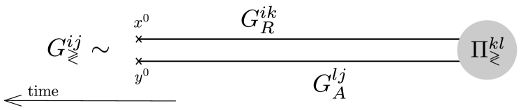
Figure 3: The information of the Wightman functions of the RH neutrinos are encoded in the self-energies $\Pi\gtrless$ in the past and transferred from the past to $t=x^{0},y^{0}$ by the retarded and advanced Green functions.

These equations mean that the information of the distribution function of the RH neutrinos in the Wightman functions $G_{\gtrless}^{ij}$ are encoded in the self-energies $\Pi_{\gtrless}^{kl}$ in the past, and transferred from the past to the present $t=x^{0},y^{0}.$ The self-energies $\Pi_{\gtrless}^{kl}$ encode the information of the distributions functions of the SM leptons and the Higgs in the past (see Fig.3). In the flavor diagonal case of (3.50), all flavors of the RH neutrinos are the same in the leading order approximation. On the other hand, in the flavor off-diagonal case of (3.51), the flavor oscillation plays an important role.

Here we note that, as shown in (3.38) and (3.39), $G_{R/A}^{{}^{\prime}ij}$ is a coherent sum of two terms, each of which corresponds to a propagation of the $i$-th (or $j$-th) flavor RH neutrino. We divide it as follows:

$$G_{R}^{{}^{\prime}ij}={\big{[}}G_{R}^{{}^{\prime}ij}{\big{]}}_{i}+{\big{[}}G_{R}^{{}^{\prime}ij}{\big{]}}_{j}\ .$$ (6.1)

A precise definition is given in (M.91).

6.1 On-shell and off-shell separation of $G_{\gtrless}^{{}^{\prime}(eq)}$

Now let’s investigate $G_{\tiny\raisebox{-0.5pt}[0.0pt][0.0pt]{$\stackrel{{\scriptstyle\textstyle>}}{{\textstyle\rule{0.0pt}{1.5pt}\smash{<}}}$}}^{{}^{\prime}ij}$. By looking at the first term of (3.51), it contains $G_{A}^{djj}$ which describes the propagation of the $j$-th RH neutrino. The propagator $G_{R}^{{}^{\prime}ij}$ in the first term contains both of the propagations of $i$-th and $j$-th flavor neutrinos. If the $j$-th neutrino propagates in $G_{R}^{{}^{\prime}ij}$, only a single ($j$-th) neutrino propagates from the past, when the decay/inverse-decay represented by $\Pi_{\gtrless}$ takes place, to the present at $t=x^{0},y^{0}.$ We call this type of contributions the “on-shell” contributions. These contributions are all taken into account in the classical Boltzmann equation.

On the contrary, if the $i$-th neutrino propagates in $G_{R}^{{}^{\prime}ij}$, two different flavors propagate from the past to the present. This type of contributions are essentially “off-shell”. In the classical Boltzmann equation, we first calculate the S-matrix elements of various processes and the external lines are taken to be on-shell. Hence this type of “off-shell” contributions are not taken into account by ordinary methods. Separation of various Green functions, especially $\Delta G_{\gtrless}^{{}^{\prime}ij}$, are calculated in Appendix M.

For $G_{\gtrless}^{{}^{\prime}}$ in eq.(3.51), on-shell contributions come from $j$-th propagation ${\big{[}}G^{{}^{\prime}ij}_{R}{\big{]}}_{j}$ of $G_{R}^{{}^{\prime}ij}$ in the first term and the $i$-th propagation ${\big{[}}G^{{}^{\prime}ij}_{A}{\big{]}}_{i}$ of $G_{A}^{{}^{\prime}ij}$ in the second term. All the other terms, $i$-th propagation ${\big{[}}G^{{}^{\prime}ij}_{R}{\big{]}}_{i}$ of $G_{R}^{{}^{\prime}ij}$ in the first term, the $j$-th propagation ${\big{[}}G^{{}^{\prime}ij}_{A}{\big{]}}_{j}$ of $G_{A}^{{}^{\prime}ij}$ in the second term give the off-shell contributions. The third term is off-shell since different mass eigenstates propagate in $G_{R}^{dii}$ and $G_{A}^{djj}$. $G_{R}^{{}^{\prime}(eq)}$ is separated into

$$G_{R}^{{}^{\prime}(eq)}={\big{[}}G_{R}^{{}^{\prime}(eq)}{\big{]}}_{\mbox{on-shell}}+{\big{[}}G_{R}^{{}^{\prime}(eq)}{\big{]}}_{\mbox{off-shell}}\ .$$ (6.2)

If we neglect the off-shell terms and take only the on-shell terms, ${\big{[}}G_{R}^{{}^{\prime}(eq)}{\big{]}}_{\mbox{on-shell}}$ becomes ($x^{0}>y^{0}$)

$${\big{[}}G^{{}^{\prime}(eq)ij}_{\tiny\raisebox{-0.5pt}[0.0pt][0.0pt]{$\stackrel{{\scriptstyle\textstyle>}}{{\textstyle\rule{0.0pt}{1.5pt}\smash{<}}}$}}(x^{0},y^{0};{\mathbb{q}}){\big{]}}_{\mbox{on-shell}}$$

$$=\sum_{\epsilon}Z_{\epsilon}\Pi^{{}^{\prime}(eq)ij}_{R}(\epsilon\omega_{q})Z_{\epsilon}\frac{+i}{\Omega_{\epsilon i}-\Omega_{\epsilon j}}(-i)\left\{\begin{matrix}1-f^{\epsilon}_{jq}\\ -f^{\epsilon}_{jq}\end{matrix}\right\}e^{-i\Omega_{\epsilon j}(x^{0}-y^{0})}$$

$$\hskip 10.0pt+\sum_{\epsilon}Z_{\epsilon}\Pi^{{}^{\prime}(eq)ij}_{A}(\epsilon\omega_{q})Z_{\epsilon}\frac{-i}{\Omega^{*}_{\epsilon i}-\Omega^{*}_{\epsilon j}}(-i)\left\{\begin{matrix}1-f^{\epsilon}_{iq}\\ -f^{\epsilon}_{iq}\end{matrix}\right\}e^{-i\Omega_{\epsilon i}(x^{0}-y^{0})}\ .$$ (6.3)

Note that the sum of the on-shell contributions do not vanish even at $x^{0}=y^{0}$ and $f_{i}\simeq f_{j}$:

$$\lim_{x^{0}\rightarrow y^{0}}{\big{[}}G^{{}^{\prime}(eq)ij}_{\tiny\raisebox{-0.5pt}[0.0pt][0.0pt]{$\stackrel{{\scriptstyle\textstyle>}}{{\textstyle\rule{0.0pt}{1.5pt}\smash{<}}}$}}(x^{0},y^{0};{\mathbb{q}}){\big{]}}_{\mbox{on-shell}}\neq 0\ .$$ (6.4)

It is different from the property of the full contributions given in (3.59).

6.2 On-shell and off-shell separation of $\Delta G_{\gtrless}^{{}^{\prime}}$

We next investigate $\Delta G_{\gtrless}^{{}^{\prime}}$. We show that neglecting the off-shell contribution in $\Delta G_{\gtrless}^{{}^{\prime}}$, we get an enhancement factor for the $CP$-violating parameter with a regulator $|M_{i}\Gamma_{i}-M_{j}\Gamma_{j}|$.

In Appendix M.7, we separate $\Delta G_{\gtrless}^{{}^{\prime}}$ into on-shell and off-shell contributions:

$$\Delta G_{\gtrless}^{{}^{\prime}}={\big{[}}\Delta G^{{}^{\prime}ij}_{\tiny\raisebox{-0.5pt}[0.0pt][0.0pt]{$\stackrel{{\scriptstyle\textstyle>}}{{\textstyle\rule{0.0pt}{1.5pt}\smash{<}}}$}}{\big{]}}_{\mbox{on-shell}}+{\big{[}}\Delta G^{{}^{\prime}ij}_{\tiny\raisebox{-0.5pt}[0.0pt][0.0pt]{$\stackrel{{\scriptstyle\textstyle>}}{{\textstyle\rule{0.0pt}{1.5pt}\smash{<}}}$}}{\big{]}}_{\mbox{off-shell}}\ .$$ (6.5)

The full $\Delta G_{\gtrless}^{{}^{\prime}}$ is given in (J.34). The on-shell contribution is given by (for $x^{0}>y^{0}$)

$${\big{[}}\Delta G^{{}^{\prime}ij}_{\tiny\raisebox{-0.5pt}[0.0pt][0.0pt]{$\stackrel{{\scriptstyle\textstyle>}}{{\textstyle\rule{0.0pt}{1.5pt}\smash{<}}}$}} (x^{0},y^{0};{\mathbb{q}}){\big{]}}_{\mbox{on-shell}}$$

$$= \sum_{\epsilon}Z_{\epsilon}\Pi^{{}^{\prime}(eq)ij}_{R}(\epsilon\omega_{q})Z_{\epsilon}(-i)\Delta\left\{\begin{matrix}1-f^{\epsilon}_{jq}\\ -f^{\epsilon}_{jq}\end{matrix}\right\}\frac{i}{\Omega_{\epsilon i}-\Omega_{\epsilon j}}\ e^{-i\Omega_{\epsilon}s_{xy}}$$

$$+\sum_{\epsilon}Z_{\epsilon}\Pi^{{}^{\prime}(eq)ij}_{A}(\epsilon\omega_{q})Z_{\epsilon}(-i)\Delta\left\{\begin{matrix}1-f^{\epsilon}_{iq}\\ -f^{\epsilon}_{iq}\end{matrix}\right\}\frac{-i}{\Omega^{*}_{\epsilon i}-\Omega^{*}_{\epsilon j}}\ e^{-i\Omega_{\epsilon}s_{xy}}\ .$$ (6.6)

This on-shell contribution has two important properties. First, it satisfies

$${\big{[}}\Delta G^{{}^{\prime}ij}_{\tiny\raisebox{-0.5pt}[0.0pt][0.0pt]{$\stackrel{{\scriptstyle\textstyle>}}{{\textstyle\rule{0.0pt}{1.5pt}\smash{<}}}$}}{\big{]}}_{\mbox{on-shell}}=\Delta{\big{[}}G^{{}^{\prime}ij}_{\tiny\raisebox{-0.5pt}[0.0pt][0.0pt]{$\stackrel{{\scriptstyle\textstyle>}}{{\textstyle\rule{0.0pt}{1.5pt}\smash{<}}}$}}{\big{]}}_{\mbox{on-shell}}$$ (6.7)

where ${\big{[}}G^{{}^{\prime}ij}_{\tiny\raisebox{-0.5pt}[0.0pt][0.0pt]{$\stackrel{{\scriptstyle\textstyle>}}{{\textstyle\rule{0.0pt}{1.5pt}\smash{<}}}$}}{\big{]}}_{\mbox{on-shell}}$ is given in (6.3). The on-shell contribution of (M.118) is simply obtained by replacing $f^{(eq)}$ by its variation $\Delta f$ in (6.3). This replacing means that the process of the flavor oscillations and the process of taking a variation from the thermal values are commutative if we neglect the off-shell contributions. For full quantum calculations, (3.60) cannot be obtained by such a replacement from (3.59). This is because the flavor oscillations and the deviation from the thermal values are coherently mixed and these processes are not commutable. Namely, dropping the off-shell contributions corresponds to neglecting the interference between the flavor oscillations and the deviation of the distribution functions from the thermal equilibrium.

Second, compared with the full result (J.34), the enhancement factor $1/(\Omega_{i}-\Omega_{j}^{*})$ is replaced by $1/(\Omega_{i}-\Omega_{j})$. It is related to the above non-commutativity of taking $\Delta$ and flavor oscillation effects.

By inserting the on-shell formula (6.3) and (M.118) into (5.5), and supposing $\pi_{\rho}(\epsilon\omega_{q})=-g_{w}i\epsilon{\ooalign{\hfil/\hfil\crcr$q$}}_{\epsilon}/(16\pi)$,  $\pi_{h}(\epsilon\omega_{q})=0$, we have an on-shell approximation ${\big{[}}{\mathcal{C}}_{\Delta f}^{{}^{\prime}}{\big{]}}_{\mbox{on-shell}}$ of ${\mathcal{C}}_{\Delta f}^{{}^{\prime}}$:

$${\big{[}}{\mathcal{C}}_{\Delta f}^{{}^{\prime}}{\big{]}}_{\mbox{on-shell}}\simeq\sum_{i=1,2} \int\frac{d^{3}p}{(2\pi)^{3}2\omega_{p}}\frac{d^{3}k}{(2\pi)^{3}2\omega_{k}}\frac{d^{3}q}{(2\pi)^{3}\omega_{q}}\ \frac{(2\pi)^{3}\delta^{3}(q-p-k)\Gamma_{\ell\phi}}{(\omega_{q}-\omega_{p}-\omega_{k})^{2}+\Gamma_{\ell\phi}^{2}/4}$$

$$g_{w}\Im(h^{{\dagger}}h)^{2}_{ij}(q\cdot p)\frac{g_{w}M^{2}}{8\pi}\frac{M^{2}_{i}-M^{2}_{j}}{(M^{2}_{i}-M^{2}_{j})^{2}+(M_{i}\Gamma_{i}-M_{j}\Gamma_{j})^{2}}$$

$$\times{\bigg{\{}}\Delta f_{iq}(1-f^{(eq)}_{\ell p})(1+f^{(eq)}_{\phi k})-\Delta(1-f_{iq})f^{(eq)}_{\ell p}f^{(eq)}_{\phi k}{\bigg{\}}}\ .$$ (6.8)

Hence the regulator $|M_{i}\Gamma_{i}+M_{j}\Gamma_{j}|$ is replace by $|M_{i}\Gamma_{i}-M_{j}\Gamma_{j}|$ if we take only the on-shell terms. It is not valid in general, especially in the resonant leptogenesis. If the masses are hierarchical, it becomes identical with the correct value in (5.11).

6.3 Summary of this section

As emphasized above, if we neglect the off-shell contributions that are not included in the ordinary Boltzmann type analysis, we get a result (6.6) which is different from the correct one given in (4.22). The only difference is the enhancement factor, and if the mass difference is much larger than the width they coincide. But the difference is enlarged when the masses are almost degenerate. This reflects the fact that the flavor oscillation becomes important only for degenerate masses. Another important point is that the property of the noncommutativity (4.25) in the full result disappears if we take only the on-shell contributions as in (6.7). The noncommutativity is related to the vanishing of $G_{\gtrless}^{{}^{\prime}}$ at the equal time (3.61). For the on-shell contributions, ${\big{[}}G_{\gtrless}^{{}^{\prime}}{\big{]}}_{\mbox{on-shell}}$ does not vanish as shown in (6.4).

Based on this observation, we give another derivation of the properties of $\Delta G_{\gtrless}^{{}^{\prime}}$ in Appendix K by directly solving the KB equations. If we assume the vanishing condition (K.70) of $G_{\gtrless}^{{}^{\prime}}$ which is equivalent to (3.61), we show that the enhancement factor with a regulator $M_{i}\Gamma_{i}+M_{j}\Gamma_{j}$ appears as in (K.71). On the other hand, if we erroneously assume that it does not vanish, it leads to a much larger enhancement factor.

7 Summary

We investigate the Kadanoff-Baym equations of the thermal resonant leptogenesis in the expanding universe. The lepton asymmetry is generated in the $CP$-asymmetric decay of the RH neutrinos which are deviated from the thermal equilibrium. If the RH neutrinos have almost degenerate masses, they coherently oscillate during their decay into the SM leptons and the Higgs. In such a situation, the classical Boltzmann equation is not valid because the decays and the inverse-decays of the RH neutrinos cannot be separated into different processes, and the full quantum mechanical approach is necessary. A systematic approach is given by solving the KB equations.

Kadanoff-Baym approach to the resonant leptogenesis was performed in the previous analysis [56]. In the paper, the authors studied the coherent oscillation of the RH neutrinos in a time-independent background with a non-equilibrium initial condition. In the process of approaching the equilibrium, the RH neutrinos coherently oscillate and decay into the SM particles. From the generated amount of the lepton number, they extracted the $CP$-violating parameter $\varepsilon_{i}$ of the $i$-th RH neutrino (1.1) and obtained the regulator $R_{ij}=|M_{i}\Gamma_{i}+M_{j}\Gamma_{j}|$. Since the resonant enhancement is the key to the resonant leptogenesis, it is essential to obtain the correct form of the regulator.

In the present paper, by extending the analysis in the static background [56] to the thermal resonant leptogenesis in the expanding universe, we obtain an analytical expression of the evolution equation of the lepton number asymmetry. The $CP$-violating parameter is obtained as in (5.24). The regulator we obtained is consistent with the result [56].

The difference between the regulator $R_{ij}=|M_{i}\Gamma_{i}+M_{j}\Gamma_{j}|$ and $R_{ij}=|M_{i}\Gamma_{i}-M_{j}\Gamma_{j}|$ obtained by [57] comes from different forms of the enhancement factors of flavor off-diagonal components of the RH neutrino propagators. Since the RH neutrinos have almost degenerate masses, they coherently oscillate very much. We show that the resonant oscillations between different flavors have two different types, one proportional to $1/(\Omega_{i}-\Omega_{j}^{*})$ and the other proportional to $1/(\Omega_{i}-\Omega_{j})$. Here $\Omega_{i}=\omega_{iq}-i\Gamma_{iq}/2$ is a position of the pole of the $i$-th RH neutrino. In the thermal equilibrium, the resonant oscillations in the flavor off-diagonal Green functions have the type $1/(\Omega_{i}-\Omega_{j})$ ( or its complex conjugate) as shown in (3.38) or in (3.60). Since $1/(\Omega_{i}-\Omega_{j})$ is rewritten by (3.49), the enhancement of flavor oscillation corresponds to the regulator $R_{ij}=|M_{i}\Gamma_{i}-M_{j}\Gamma_{j}|$. However, the deviation of the off-diagonal components of out of equilibrium has a different enhancement factor $1/(\Omega_{i}-\Omega_{j}^{*})$ as shown in (4.22), which corresponds to the regulator $R_{ij}=|M_{i}\Gamma_{i}+M_{j}\Gamma_{j}|$. Physical interpretation of the change of the regulator is given in Section 6. The off-shell contributions to the off-diagonal component to the Wightman functions are essential which can be incorporated only by the KB equations. The property (3.61) is also important for this change of the regulator. As we show in Appendix K, if we erroneously assume that the off-diagonal component of the Wightman function is non-vanishing and its deviation is given by the change of the local temperature, it leads to much more enhanced oscillation similar to the regulator $R_{ij}=|M_{i}\Gamma_{i}-M_{j}\Gamma_{j}|$.

In the present paper, we focus on the formalism of the thermal resonant leptogenesis and derivations of the $CP$-violating parameter in the expanding universe. Phenomenological investigations of the amount of the generated lepton asymmetry and the lower bound of the leptogenesis scale consistent with the neutrino oscillation data are left for future investigations.

Appendix A CTP formalism

In this appendix, we briefly review the closed time path (CTP) formalism.

In equilibrium field theories, we implicitly assume that the initial and final states asymptotically approach the ground state of the free Hamiltonian. But this does not hold in general, especially in time-dependent backgrounds such as the evolving universe. The final state is generally different from the initial state. The CTP formalism, or the Schwinger-Keldish formalism, is the general formalism to calculate physical quantities for time-dependent wave functions.

Suppose that a system is described by a Hamiltonian $\hat{H_{0}}+\hat{H_{1}}$, where $\hat{H_{0}}$ and $\hat{H_{1}}$ are free and interaction Hamiltonians, and that the system is in the initial state $|\psi_{i}\rangle$ at time $t=t_{i}$. In the interaction picture, the expectation value of an observable $\hat{\mathcal{O}}$ at time $t$ is given by

$${\mathcal{O}}(t)=\langle\psi_{i}^{I}(t)|\hat{{\mathcal{O}}}^{I}(t)|\psi_{i}^{I}(t)\rangle=\langle\psi_{i}|U^{I}(t_{i},t)\hat{{\mathcal{O}}}^{I}(t)U^{I}(t,t_{i})|\psi_{i}\rangle\ .$$ (A.1)

Here the operator in the interaction picture $\hat{{\mathcal{O}}}^{I}(t)$ is related to the operator in the Heisenberg picture as

$$\hat{{\mathcal{O}}}^{H}(t) = U^{I}(t,t_{i})\hat{{\mathcal{O}}}^{I}(t)U^{I\dagger}(t,t_{i})\ ,$$

$$U^{I}(t,t^{\prime}) = T\exp\left(-i\int_{t^{\prime}}^{t}dt^{\prime\prime}\hat{H_{1}}^{I}(t^{\prime\prime})\right)\ .$$ (A.2)

In equilibrium cases, the final state at time $t=t_{f}$ is assumed to be proportional to the initial state $U^{I}(t_{f},t_{i})|\psi_{i}\rangle=e^{i\theta}|\psi_{i}\rangle$ where $\theta(t_{f},t_{i})$ is a c-number phase. Then we can factorize ${\mathcal{O}}(t)$ of (A.1) as

$${\mathcal{O}}(t) = \langle\psi_{i}|U^{I}(t_{i},t_{f})|\psi_{i}\rangle\langle\psi_{i}|U^{I}(t_{f},t)\hat{{\mathcal{O}}}^{I}(t)U^{I}(t,t_{i})|\psi_{i}\rangle$$ (A.3)

$$= e^{-i\theta}\langle\psi_{i}|U^{I}(t_{f},t)\hat{{\mathcal{O}}}^{I}(t)U^{I}(t,t_{i})|\psi_{i}\rangle\ .$$

Similarly, an expectation value of the time-ordering product of two operators $\hat{{\mathcal{O}}}_{1}^{I}(t_{1})$ and $\hat{{\mathcal{O}}}_{2}^{I}(t_{2})$ is given by

$${\mathcal{O}}(t_{1},t_{2})=e^{-i\theta}\langle\psi_{i}|T\left(\hat{{\mathcal{O}}}_{1}^{I}(t_{1})\hat{{\mathcal{O}}}_{2}^{I}(t_{2})U^{I}(t_{f},t_{i})\right)|\psi_{i}\rangle\ .$$ (A.4)

This formula gives an ordinary perturbative expansion of correlation functions in equilibrium field theories. Namely, if we take $t_{i}\rightarrow-\infty$ and $t_{f}\rightarrow\infty$, the interaction vertices $\hat{H}^{I}(t)$ are inserted in $-\infty<t<\infty$.

In non-equilibrium cases where the final state is no longer proportional to the initial state, the factorization property does not hold and we have

$${\mathcal{O}}(t_{1},t_{2})=\langle\psi_{i}|U^{I}(t_{i},t_{f})T\left(\hat{{\mathcal{O}}}_{1}^{I}(t_{1})\hat{{\mathcal{O}}}_{2}^{I}(t_{2})U^{I}(t_{f},t_{i})\right)|\psi_{i}\rangle\ .$$ (A.5)

In perturbative expansions, the interaction vertices are inserted not only on the path ${\mathcal{C}}_{+}$ from $t_{i}$ to $t_{f}$, but also on the backward path ${\mathcal{C}}_{-}$ from $t_{f}$ to $t_{i}$. Figure 4 shows the closed time path (CTP), ${\mathcal{C}}={\mathcal{C}}_{+}+{\mathcal{C}}_{-}.$

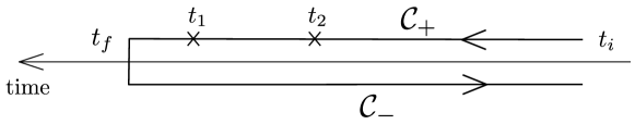
Figure 4: A closed time path ${\mathcal{C}}$ from $t_{i}$ to $t_{f}$ and then back to $t_{i}$. (i.e., ${\mathcal{C}}={\mathcal{C}}_{+}+{\mathcal{C}}_{-}$.) Operators are inserted at $t=t_{1}$ and $t_{2}$ for the time ordered product ${\mathcal{O}}(t_{1},t_{2})$. Interaction vertices are inserted everywhere on the CTP.

In this formalism, the final state is not specified at all and we can calculate time-dependence of various quantities as in (A.5). The time-ordering $T_{C}$ is defined on the CTP as a path-ordering along ${\mathcal{C}}={\mathcal{C}}_{+}+{\mathcal{C}}_{-}.$

Appendix B Evolution equations of various propagators

We define various propagators and give a brief derivation of their evolution equations. In the following we consider a real (Majorana) fermion field $\hat{\psi}$ and write its conjugate by $\overline{\hat{\psi}}=\hat{\psi}^{t}C$ where $C=i\gamma^{2}\gamma^{0}$. In the CTP formalism, a generating function of time-ordered products of operators is given by

$$Z[\overline{J}]= e^{iW[\overline{J}]}=\left\langle{\rm T}_{\mathcal{C}}\ e^{i\int_{\mathcal{C}}d^{4}x\sqrt{-g}\ \overline{J}(x)\hat{\psi}(x)}\right\rangle$$

$$= \int d\Psi_{+}d\Psi_{-}\langle\Psi_{+}|\hat{\rho}_{(t_{i})}|\Psi_{-}\rangle\int{\mathcal{D}}^{\prime}\psi\ e^{iS[\psi]+i\int_{\mathcal{C}}d^{4}x\sqrt{-g}\ \overline{J}(x)\psi(x)}$$ (B.1)

where $\hat{\rho}(t_{i})=|\psi_{i}\rangle\langle\psi_{i}|$. The path integral $\int{\mathcal{D}}^{\prime}\psi$ denotes an integration of the Grassmann variables $\psi_{\pm}$ on ${\mathcal{C}}_{\pm}$ with the fixed boundary conditions $\psi_{\pm}(t_{i})=\Psi_{\pm}$. The integrations of $\Psi_{\pm}$ represent an weighting by the initial wave function $|\psi_{i}\rangle$. The source $\overline{J}(x)$ is defined on ${\mathcal{C}}={\mathcal{C}}_{+}+{\mathcal{C}}_{-}$. The 1PI effective action is obtained from the generating function $W[\overline{J}]$ of the connected Green function by the Legendre transformation. Defining the classical field by the left-derivative of $W[\overline{J}]$ with respect to the Grassmannian source $\overline{J}$:

$$\Psi(x)=+\frac{\delta W[\overline{J}]}{\delta\overline{J}(x)}\ ,$$ (B.2)

we have

$$\Gamma[\Psi]=W[\overline{J}]-\int_{\mathcal{C}}d^{4}x_{g}\overline{J}(x)\Psi(x)\ .$$ (B.3)

For notational simplicity, we use the following abbreviation

$$d^{4}x_{g}\equiv d^{4}x\sqrt{-g(x)}$$ (B.4)

unless the explicit dependence of the measure on $x$ is necessary. The stationary condition $(\delta/\delta\Psi(x))\Gamma[\Psi]=0$ at $\overline{J}=0$ gives the equation of motion of $\Psi$.

By taking the second derivative of the effective action $\Gamma$ with respect to $\Psi$, we obtain the Schwinger-Dyson (SD) equation

$$iG^{-1}(x,y)=iG^{-1}_{0}(x,y)-i\Pi(x,y)\ .$$ (B.5)

$\Pi$ is the self-energy and only 1PI diagrams contribute to it. The connected Green function $G$ on ${\mathcal{C}}$ is defined by

$$G(x,y)= \ \langle{\rm T}_{\mathcal{C}}\hat{\psi}(x)\overline{\hat{\psi}}(y)\rangle$$

$$= \ {\rm\Theta}_{\mathcal{C}}(x^{0}-y^{0})G_{>}(x,y)+{\rm\Theta}_{\mathcal{C}}(y^{0}-x^{0})G_{<}(x,y)\ ,$$ (B.6)

where $\Theta_{C}(x^{0}-y^{0})$ is the step function on ${\mathcal{C}}$ and

$$G_{<}(x,y)\equiv-\langle\overline{\hat{\psi}}(y)\hat{\psi}(x)\rangle\ ,\ \ G_{>}(x,y)\equiv\langle\hat{\psi}(x)\overline{\hat{\psi}}(y)\rangle$$ (B.7)

are the Wightman Green functions. $iG^{-1}_{0}(x,y)=iG_{0(x)}^{-1}\delta^{g}_{\mathcal{C}}(x-y)$ is an inverse of the free propagator and $\Pi(x,y)$ is the self-energy of the fermion field $\psi$.

The statistical propagator $G_{F}(x,y)$ and the spectral function $G_{\rho}(x,y)$ are defined by

$$G_{F}(x,y)= \ \frac{1}{2}\left(G_{>}(x,y)+G_{<}(x,y)\right)=\frac{1}{2}\langle[\hat{\psi}(x),\overline{\hat{\psi}}(y)]\rangle\ ,$$ (B.8)

$$G_{\rho}(x,y)= \ i\left(G_{>}(x,y)-G_{<}(x,y)\right)=i\langle\{\hat{\psi}(x),\overline{\hat{\psi}}(y)\}\rangle\ .$$ (B.9)

$G_{F}$ contains information of the distribution function of the specified state while $G_{\rho}$ depends only on the spectrum of the system. In this sense, $G_{F}$ is dynamical while $G_{\rho}$ is kinematical. Especially, $G_{\rho}(x,y)$ becomes proportional to the spatial delta-function $\delta^{(3)}({\bf x}-{\bf y})$ in the equal-time limit. We further define the retarded and advanced Green functions by

$$G_{R/A}(x,y)=\pm\Theta(\pm(x^{0}-y^{0}))G_{\rho}(x,y).$$ (B.10)

They are related to $G_{\rho}$ as

$$G_{R}(x,y)-G_{A}(x,y) = G_{\rho}(x,y)\ ,$$

$$G_{R}(x,y)+G_{A}(x,y) = {\rm sign}(x^{0}-y^{0})G_{\rho}(x,y)\ .$$ (B.11)

In terms of $G_{F}$ and $G_{\rho}$, the Green function (B.6) can be written as

$$G(x,y)= G_{F}(x,y)-\frac{i}{2}{\rm sign}_{\mathcal{C}}(x^{0}-y^{0})G_{\rho}(x,y)\ ,$$ (B.12)

where the sign-function on ${\mathcal{C}}$ is defined by

$${\rm sign}_{\mathcal{C}}(x^{0}-y^{0})=\Theta_{\mathcal{C}}(x^{0}-y^{0})-\Theta_{\mathcal{C}}(y^{0}-x^{0})\ .$$ (B.13)

By convoluting (B.5) with the full propagator $G$, we have

$$iG_{0(x)}^{-1}G(x,y)-i\int_{\mathcal{C}}d^{4}z_{g}\ \Pi(x,z)G(z,y)=i\delta^{g}_{\mathcal{C}}(x-y)\ .$$ (B.14)

Here $\delta^{g}_{\mathcal{C}}(x-y)$ is the delta-function on $\mathcal{C}$ with the space-time metric $g$, and satisfies $\int_{C}d^{4}z_{g}\delta^{g}_{\mathcal{C}}(x-y)=1.$ By denoting $x$ on ${\mathcal{C}}_{\pm}$ as $x_{\pm}$ respectively, the delta-function on ${\mathcal{C}}$ can be expressed by a $2\times 2$ matrix:

$$\delta^{g}_{\mathcal{C}}(x_{a}-y_{b})=c_{ab}\delta^{g}(x-y)\ ,\ \ \ c_{ab}={\rm diag}(1,-1)$$ (B.15)

where $a,b$ takes $+$ or $-$. The minus sign on ${\mathcal{C}}_{-}$ comes from the backward integral of the time variable and corresponds to the anti-time-ordering of the Green function $G$ in (B.6). $\delta^{g}(x-y)$ is an ordinary delta-function for $(x-y)$.

The 2-point function $G(x,y)$ of (B.6) with $x,y\in{\mathcal{C}}$ can be similarly decomposed (depending on whether $x,y$ are on ${\mathcal{C}}_{+}$ or ${\mathcal{C}}_{-}$) into a $2\times 2$ matrix form as

$$G_{ab}(x,y)=\left(\begin{matrix}G_{++}(x,y)&G_{+-}(x,y)\\ G_{-+}(x,y)&G_{--}(x,y)\end{matrix}\right)=\left(\begin{matrix}G_{\rm T}(x,y)&G_{<}(x,y)\\ G_{>}(x,y)&G_{\widetilde{\rm T}}(x,y)\end{matrix}\right)$$ (B.16)

where ${\rm T},\widetilde{{\rm T}}$ denote time and anti-time orderings respectively, and

$$G_{\rm T}(x,y) =\ \Theta(x^{0}-y^{0})G_{>}(x,y)+\Theta(y^{0}-x^{0})G_{<}(x,y)\ ,$$

$$G_{\widetilde{\rm T}}(x,y) =\ \Theta(x^{0}-y^{0})G_{<}(x,y)+\Theta(y^{0}-x^{0})G_{>}(x,y)\ .$$ (B.17)

$\Theta(x^{0}-y^{0})$ is the ordinary step-function. By using (B.12) and (B.11), we have

$$G_{ab}(x,y) = \left(\begin{matrix}G_{F}-\frac{i}{2}{\rm sign}(x^{0}-y^{0})G_{\rho}&G_{F}+\frac{i}{2}G_{\rho}\\ G_{F}-\frac{i}{2}G_{\rho}&G_{F}+\frac{i}{2}{\rm sign}(x^{0}-y^{0})G_{\rho}\end{matrix}\right)$$ (B.18)

$$= \left(\begin{matrix}G_{F}-\frac{i}{2}(G_{R}+G_{A})&G_{F}+\frac{i}{2}(G_{R}-G_{A})\\ G_{F}-\frac{i}{2}(G_{R}-G_{A})&G_{F}+\frac{i}{2}(G_{R}+G_{A})\end{matrix}\right)$$

$$= U^{t}\left(\begin{matrix}0&G_{A}\\ G_{R}&G_{F}\end{matrix}\right)U$$

where

$$U\equiv\left(\begin{matrix}-i/2&i/2\\ 1&1\end{matrix}\right)\ .$$ (B.19)

We also decompose the self-energy $\Pi(x,y)$ as

$$\Pi(x,y)= \ {\rm\Theta}_{\mathcal{C}}(x^{0}-y^{0})\Pi_{>}(x,y)+{\rm\Theta}_{\mathcal{C}}(y^{0}-x^{0})\Pi_{<}(x,y)$$

$$= \ \Pi_{F}(x,y)-\frac{i}{2}{\rm sign}_{\mathcal{C}}(x^{0}-y^{0})\Pi_{\rho}(x,y)\ .$$ (B.20)

Defining $\Pi_{R/A}$ by

$$\Pi_{R/A}(x,y)=\pm\Theta(\pm(x^{0}-y^{0}))\Pi_{\rho}(x,y)\ ,$$ (B.21)

the matrix form of the self-energy is obtained as

$$\Pi_{ab}=\left(\begin{matrix}\Pi_{\rm T}&\Pi_{<}\\ \Pi_{>}&\Pi_{\widetilde{\rm T}}\end{matrix}\right)=U^{t}\left(\begin{matrix}0&\Pi_{A}\\ \Pi_{R}&\Pi_{F}\end{matrix}\right)U\ .$$ (B.22)

Using these matrix forms of $G_{ab}$ and $\Pi_{ab}$, the equation (B.14) becomes

$$iG_{0(x)}^{-1}G_{ab}(x,y)-i\int_{t_{i}}^{t_{f}}d^{4}z_{g}\ \Pi_{ac}(x,z)c_{cd}G_{db}(z,y)=i\delta^{g}(x-y)c_{ab}\ .$$ (B.23)

The matrix $c_{cd}$ between $\Pi$ and $G$ comes from the backward integration of the time variable in the original integral in (B.14). By multiplying $(U^{t})^{-1}$ on the left and $U^{-1}$ on the right, using (B.18) and (B.22) and noting

$$Uc\ U^{t}=\left(\begin{matrix}0&-i\\ -i&0\end{matrix}\right)\ ,$$ (B.24)

we obtain the following set of the evolution equations:

$$iG_{0(x)}^{-1}G_{F}(x,y)-\int^{\infty}_{t_{int}}d^{4}z_{g}\ \Pi_{R}(x,z)G_{F}(z,y)-\int^{\infty}_{t_{int}}d^{4}z_{g}\ \Pi_{F}(x,z)G_{A}(z,y)=0\ ,$$ (B.25)

$$iG_{0(x)}^{-1}G_{R/A}(x,y)-\int^{\infty}_{t_{int}}d^{4}z_{g}\ \Pi_{R/A}(x,z)G_{R/A}(z,y) =-\delta^{g}(x-y)\ .$$ (B.26)

From the equations (B.26), we obtain the evolution equation for the spectral density $G_{\rho}=G_{R}-G_{A}$:

$$iG_{0(x)}^{-1}G_{\rho}(x,y) -\int^{\infty}_{t_{int}}d^{4}z_{g}\ \Pi_{R}(x,z)G_{\rho}(z,y)-\int^{\infty}_{t_{int}}d^{4}z_{g}\ \Pi_{\rho}(x,z)G_{A}(z,y)=0\ .$$ (B.27)

The Wightman Green function $G_{\tiny\raisebox{-0.5pt}[0.0pt][0.0pt]{$\stackrel{{\scriptstyle\textstyle>}}{{\textstyle\rule{0.0pt}{1.5pt}\smash{<}}}$}}=G_{F}\mp(i/2)G_{\rho}$ satisfies

$$iG_{0(x)}^{-1}G_{\tiny\raisebox{-0.5pt}[0.0pt][0.0pt]{$\stackrel{{\scriptstyle\textstyle>}}{{\textstyle\rule{0.0pt}{1.5pt}\smash{<}}}$}}(x,y) -\int^{\infty}_{t_{int}}d^{4}z_{g}\ \Pi_{R}(x,z)G_{\tiny\raisebox{-0.5pt}[0.0pt][0.0pt]{$\stackrel{{\scriptstyle\textstyle>}}{{\textstyle\rule{0.0pt}{1.5pt}\smash{<}}}$}}(z,y)-\int^{\infty}_{t_{int}}d^{4}z_{g}\ \Pi_{\tiny\raisebox{-0.5pt}[0.0pt][0.0pt]{$\stackrel{{\scriptstyle\textstyle>}}{{\textstyle\rule{0.0pt}{1.5pt}\smash{<}}}$}}(x,z)G_{A}(z,y)=0\ .$$ (B.28)

Appendix C 2PI formalism

In this appendix, we give a brief review of a systematic approach to evaluate the self-energy based on the 2PI formalism (see, e.g., [92] for more details). The generating functional $Z[\overline{J},R]$ in the presence of sources $J(x)$ and $R(x,y)$ is given by

$$Z[\overline{J},R]= e^{iW[\overline{J},R]}$$

$$= \left\langle{\rm T}_{\mathcal{C}}\ e^{i\int_{\mathcal{C}}d^{4}x_{g}\ \overline{J}(x)\hat{\psi}(x)+\frac{i}{2}\int_{\mathcal{C}}d^{4}x_{g}d^{4}y_{g}\ \overline{\hat{\psi}}(x)R(x,y)\hat{\psi}(y)}\right\rangle\ .$$ (C.1)

By taking a variation with respect to the source fields $J(x)$ and $R(y,x)$, we have

$$\frac{\delta W[\overline{J},R]}{\delta\overline{J}_{\zeta}(x)} =+\Psi_{\zeta}(x)\ ,$$

$$\frac{\delta W[\overline{J},R]}{\delta R_{\eta\zeta}(y,x)} =-\frac{1}{2}\left(\Psi_{\zeta}(x)\overline{\Psi}_{\eta}(y)+G_{\zeta\eta}(x,y)\right)\ .$$ (C.2)

Here $\zeta,\eta$ represent Spinor indices.

$\overline{\Psi}$ is defined as $\overline{\Psi}(x)\equiv\Psi^{t}(x)C$ and the connected Green function $G$ is given by

$$G_{\zeta\eta}(x,y)=i\frac{\delta^{2}W[\overline{J},R]}{\delta\overline{J}_{\zeta}(x)\delta J_{\eta}(y)}\ .$$ (C.3)

By taking the Legendre transform of $W[\overline{J},R]$ with respect to the sources $J,R$, we obtain the effective action in the presence of source fields

$$\Gamma[\Psi,G] \equiv W[\overline{J},R]-\int_{\mathcal{C}}d^{4}x_{g}\ \overline{J}_{\zeta}(x)\frac{\delta W[\overline{J},R]}{\delta\overline{J}_{\zeta}(x)}-\int_{\mathcal{C}}d^{4}x_{g}d^{4}y_{g}R_{\zeta\eta}(x,y)\frac{\delta W[\overline{J},R]}{\delta R_{\zeta\eta}(x,y)}$$

$$=W[\overline{J},R]-\int_{\mathcal{C}}d^{4}x_{g}\overline{J}\Psi-\frac{1}{2}\int_{\mathcal{C}}d^{4}x_{g}d^{4}y_{g}\overline{\Psi}(x)R(x,y)\Psi(y)+\frac{1}{2}{\rm Tr}GR\ .$$ (C.4)

${\rm Tr}$ in the last term represents a trace in the Spinor indices and an integration over the closed time path ${\mathcal{C}}$.

Now we decompose the effective action into

$$\Gamma[\Psi,G]=S(\Psi) -\frac{i}{2}{\rm Tr}\ln G^{-1}-\frac{i}{2}{\rm Tr}G_{0}^{-1}G+\Gamma_{2}[\Psi,G]\ .$$ (C.5)

The first term is the classical action. The second and the third term are ‘1-loop’ type contributions to the effective action. The meaning of the decomposition can be understood by taking a functional derivative with respect to $G$:

$$\left.\frac{\delta\Gamma[\Psi,G]}{\delta G_{\eta\zeta}(y,x)}\right|_{R=0}=\frac{i}{2}G_{\zeta\eta}^{-1}(x,y)-\frac{i}{2}G_{0,\zeta\eta}^{-1}(x,y)+\frac{\delta\Gamma_{2}(\Psi,G)}{\delta G_{\eta\zeta}(y,x)}=0\ .$$ (C.6)

Compared with the SD equation (B.5), the last term can be identified as the self-energy $\Pi$:

$$\Pi_{\zeta\eta}(x,y;\Psi,G) =-2i\frac{\delta\Gamma_{2}(\Psi,G)}{\delta G_{\eta\zeta}(y,x)}\ .$$ (C.7)

In this way, the proper self-energy $\Pi$ is obtained by differentiating $\Gamma_{2}$ with respect to the full propagator $G$. Since the proper self-energy $\Pi$ is calculated as a sum of contributions from 1PI diagrams, $\Gamma_{2}$ becomes a sum of contributions from 2PI diagrams with respect to the full propagator. In another word, the proper self-energy can be systematically obtained by taking a functional derivative of 2PI diagrams (in which all internal lines are full propagators) with respect to the full propagator.

The SD equation (C.6) can be interpreted as a self-consistent equation for the full propagators. By rewriting this equation on the forward time line ${\mathcal{C}}_{+}$, we obtain the set of KB equations (B.25), (B.26), (B.27), (B.28) which can be interpreted as equations for the full propagators.

For Dirac or Weyl fermions, we introduce additional source terms

$$+i\int_{\mathcal{C}}d^{4}x_{g}\ \overline{\hat{\psi}}(x)J(x)+i\int_{\mathcal{C}}d^{4}xd^{4}y\ \overline{\hat{\psi}}(x)R(x,y)\hat{\psi}(y)\ .$$

The self-energy is similarly obtained as a functional of the full propagators:

$$\Pi_{\zeta\eta}(x,y;\Psi,\overline{\Psi},G) =-i\frac{\delta\Gamma_{2}(\Psi,\overline{\Psi},G)}{\delta G_{\eta\zeta}(y,x)}\ .$$ (C.8)

Appendix D Self-energies $\Sigma,\Pi$

In this appendix, using the 2PI formalism, we give an expression of the self-energy function for the RH neutrino $\Pi(x,y)$ in terms of the lepton and Higgs propagators. The simplest and the most important contribution to the 2PI effective action $\Gamma_{2}$ in the model (2.4) is given by the 2-loop diagram of Figure 2.

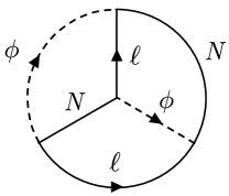
Figure 5: Another example of 2PI diagrams.

The second simplest 2PI diagram is given by Figure 5. Note that each internal line represents a full propagator of the SM lepton, Higgs and the RH neutrino. If the RH neutrinos have almost degenerate mass, we need to use the resummed propagators for the RH neutrinos. Once resummed, we can use an ordinary perturbative expansion with respect to the Yukawa coupling $h_{i\alpha}$. Hence it will not be a bad approximation to use the simplest 2PI diagram to evaluate the self-energy.

In terms of the full propagators, the contribution from the diagram Figure 2 becomes

$$\Gamma_{2}^{({\rm 2loop})}[G,S,\Delta]= \ \frac{i}{2}h^{{\dagger}}_{i\alpha}h_{\beta j}\int_{\mathcal{C}}d^{4}w_{g}d^{4}z_{g}\ \epsilon_{a^{\prime}a}\epsilon_{bb^{\prime}}\Delta_{a^{\prime}b^{\prime}}(w,z)$$

$$\times{\rm tr}\left[P_{\rm R}\left(G^{ji}(z,w)+CG^{t,ij}(w,z)C^{-1}\right)P_{\rm L}S^{\alpha\beta}_{ab}(w,z)\right]\ .$$ (D.1)

Here $G,S,\Delta$ are full propagators of the RH neutrino, the SM lepton doublet and the Higgs doublet respectively. $(i,j),(\alpha,\beta),(a,b,a^{\prime},b^{\prime})$ represent the flavor indices of the RH neutrino, the flavor indices of the leptons and the $SU(2)_{L}$ indices of the SM doublets respectively.

By using the formula (C.8), the self-energy of the SM lepton doublet is given by taking a functional derivative of $\Gamma_{2}$ with respect to the lepton propagator $S$:

$$\Sigma^{\alpha\beta}_{ab}(x,y)= \ h_{\alpha i}h^{{\dagger}}_{j\beta}P_{\rm R}G^{ij}(x,y)P_{\rm L}\epsilon_{aa^{\prime}}\epsilon_{b^{\prime}b}\Delta_{b^{\prime}a^{\prime}}(y,x)$$

$$= -\delta_{ab}h_{\alpha i}h^{{\dagger}}_{j\beta}P_{\rm R}G^{ij}(x,y)P_{\rm L}\Delta(y,x)\ .$$ (D.2)

Here we have used the Majorana property $G^{ij}(x,y)=CG^{tji}(y,x)C^{-1}$ of the RH neutrinos. In the second equality, we have used the fact that the lepton and the Higgs propagators are $SU(2)_{L}$ symmetric and proportional to $\delta_{ab}$, $S_{ab}=S\delta_{ab},\Delta_{ab}=\Delta\delta_{ab}$, in the early universe where the $SU(2)_{L}$ symmetry is restored. This is indeed the case in the era of the lepton asymmetry generation through the decay of the RH neutrino. Similarly the self-energy of the RH neutrino is obtained by taking a functional derivative of $\Gamma_{2}$ with respect to $G$:

$$\Pi^{ij}(x,y)= {\large\{}h^{{\dagger}}_{i\alpha}h_{\beta j}P_{\rm L}S^{\alpha\beta}_{ab}(x,y)P_{\rm R}\Delta_{a^{\prime}b^{\prime}}(x,y)$$

$$\ +h^{{\dagger}}_{j\alpha}h_{\beta i}P_{\rm R}P\overline{S}^{\beta\alpha}_{ba}(\overline{x},\overline{y})PP_{\rm L}\overline{\Delta}_{b^{\prime}a^{\prime}}(\overline{x},\overline{y}){\large\}}\epsilon_{a^{\prime}a}\epsilon_{bb^{\prime}}$$

$$= -g_{w}h^{{\dagger}}_{i\alpha}h_{\beta j}P_{\rm L}S^{\alpha\beta}(x,y)P_{\rm R}\Delta(x,y)$$

$$\ -g_{w}(h^{{\dagger}}_{i\alpha}h_{\beta j})^{*}P_{\rm R}P\overline{S}^{\alpha\beta}(\overline{x},\overline{y})PP_{\rm L}\overline{\Delta}(\overline{x},\overline{y})\$$ (D.3)

where $P=\gamma^{0}$. In the first equality, we have used

$$\overline{S}^{\beta\alpha}_{ba}(\overline{x},\overline{y})=CPS^{t\alpha\beta}_{\ ab}(y,x)(CP)^{-1}\ ,\ \ \overline{\Delta}_{ba}(\overline{x},\overline{y})=\Delta_{ab}(y,x)\ .$$ (D.4)

In the second equality, $SU(2)_{L}$ symmetry of $S$ and $\Delta$ is used. Decomposing these self-energies into the Wightman functions as in (B.20), we have

$$\Sigma^{\alpha\beta}_{ab\ \tiny\raisebox{-0.5pt}[0.0pt][0.0pt]{$\stackrel{{\scriptstyle\textstyle>}}{{\textstyle\rule{0.0pt}{1.5pt}\smash{<}}}$}}(x,y)= -\delta_{ab}h_{\alpha i}h^{{\dagger}}_{j\beta}P_{\rm R}G_{\tiny\raisebox{-0.5pt}[0.0pt][0.0pt]{$\stackrel{{\scriptstyle\textstyle>}}{{\textstyle\rule{0.0pt}{1.5pt}\smash{<}}}$}}^{ij}(x,y)P_{\rm L}\Delta_{\tiny\raisebox{-0.5pt}[0.0pt][0.0pt]{$\stackrel{{\scriptstyle\textstyle<}}{{\textstyle\rule{0.0pt}{1.5pt}\smash{>}}}$}}(y,x)\equiv\ \delta_{ab}\Sigma^{\alpha\beta}_{\tiny\raisebox{-0.5pt}[0.0pt][0.0pt]{$\stackrel{{\scriptstyle\textstyle>}}{{\textstyle\rule{0.0pt}{1.5pt}\smash{<}}}$}}(x,y)\ ,$$ (D.5)

$$\Pi^{ij}_{\tiny\raisebox{-0.5pt}[0.0pt][0.0pt]{$\stackrel{{\scriptstyle\textstyle>}}{{\textstyle\rule{0.0pt}{1.5pt}\smash{<}}}$}}(x,y)= -g_{w}h^{{\dagger}}_{i\alpha}h_{\beta j}P_{\rm L}S_{\tiny\raisebox{-0.5pt}[0.0pt][0.0pt]{$\stackrel{{\scriptstyle\textstyle>}}{{\textstyle\rule{0.0pt}{1.5pt}\smash{<}}}$}}^{\alpha\beta}(x,y)P_{\rm R}\Delta_{\tiny\raisebox{-0.5pt}[0.0pt][0.0pt]{$\stackrel{{\scriptstyle\textstyle>}}{{\textstyle\rule{0.0pt}{1.5pt}\smash{<}}}$}}(x,y)$$

$$\ -g_{w}(h^{{\dagger}}_{i\alpha}h_{\beta j})^{*}P_{\rm R}P\overline{S}_{\tiny\raisebox{-0.5pt}[0.0pt][0.0pt]{$\stackrel{{\scriptstyle\textstyle>}}{{\textstyle\rule{0.0pt}{1.5pt}\smash{<}}}$}}^{\alpha\beta}(\overline{x},\overline{y})PP_{\rm L}\overline{\Delta}_{\tiny\raisebox{-0.5pt}[0.0pt][0.0pt]{$\stackrel{{\scriptstyle\textstyle>}}{{\textstyle\rule{0.0pt}{1.5pt}\smash{<}}}$}}(\overline{x},\overline{y})\ .$$ (D.6)

In the following, we derive the self-energy of the RH neutrino $\Pi^{(eq)}$ under an assumption that the lepton and the Higgs are in the thermal equilibrium. The approximation is justified in the leading order calculation since the SM leptons and the Higgs particles interact faster than the Hubble expansion rate in the era of the leptogenesis. See (2.63). Hence the deviation from the equilibrium can be neglected in the calculation of $\Pi$. In the equilibrium, the lepton and the Higgs propagators become $CP$-symmetric and satisfy

$$\overline{S}(x,y)=S(x,y)\ ,\ \ \ \overline{\Delta}(x,y)=\Delta(x,y)\ .$$ (D.7)

By using the quasi-particle approximation for the propagators (2.57) and (2.58), the Fourier transform of the self-energy $\Pi_{\rho}=i(\Pi_{>}-\Pi_{<})=\Pi_{R}-\Pi_{A}$ of the RH neutrino becomes

$$\Pi^{(eq)ij}_{\rho}(q)= \left(\Re(h^{{\dagger}}h)_{ij}-i\Im(h^{{\dagger}}h)_{ij}\gamma_{5}\right)\pi^{(eq)}_{\rho}(q)\ ,$$ (D.8)

where

$$\pi^{(eq)}_{\rho}(q)= (-g_{w})\sum_{\epsilon_{\ell},\epsilon_{\phi}}\int\frac{d^{3}p}{(2\pi)^{3}2\omega_{p}}\frac{d^{3}k}{2\omega_{k}}\ \delta^{3}(q-p-k)$$

$$\times\frac{i\Gamma_{\ell\phi}}{(q_{0}-\epsilon_{\ell}\omega_{p}-\epsilon_{\phi}\omega_{k})^{2}+\Gamma_{\ell\phi}^{2}/4}\ {\ooalign{\hfil/\hfil\crcr$p$}}_{\epsilon_{\ell}}{\mathcal{D}}_{\rho(p,k)}^{\epsilon_{\ell}.\epsilon_{\phi}(eq)}\ .$$ (D.11)

${\mathcal{D}}_{\rho(p,k)}$ is given by

$${\mathcal{D}}_{\rho(p,k)}^{\epsilon_{\ell}\epsilon_{\phi}}\equiv{\mathcal{D}}_{>(p,k)}^{\epsilon_{\ell}\epsilon_{\phi}}-{\mathcal{D}}_{<(p,k)}^{\epsilon_{\ell}\epsilon_{\phi}}=(-1)^{\epsilon_{\ell}}(-1)^{\epsilon_{\phi}}\left(1-f_{\ell p}^{\epsilon_{\ell}}+f_{\phi k}^{\epsilon_{\phi}}\right)$$ (D.12)

with the definition of ${\mathcal{D}}_{\gtrless(p,k)}$ in (2.69), and satisfy the relation ${\mathcal{D}}_{\rho(p,k)}^{-\epsilon_{\ell}-\epsilon_{\phi}(eq)}=-{\mathcal{D}}_{\rho(p,k)}^{+\epsilon_{\ell}+\epsilon_{\phi}(eq)}$ and is followed by the relation of

$$\pi^{(eq)}_{\rho}(-q_{0},{\mathbb{q}})=+\gamma^{0}\pi^{(eq)}_{\rho}(+q_{0},{\mathbb{q}})\gamma^{0}\ .$$ (D.13)

In the calculation we have used the integral (in the limit $t_{int}\rightarrow-\infty$)

$$2\int_{-\infty}^{t}d\tau e^{i(-q^{0}+\epsilon_{\ell}\omega_{p}+\epsilon_{\phi}\omega_{k}+i\Gamma_{\ell\phi}/2)(t-\tau)}=\frac{\Gamma_{\ell\phi}-2i(q^{0}-\epsilon_{\ell}\omega_{p}-\epsilon_{\phi}\omega_{k})}{(q^{0}-\epsilon_{\ell}\omega_{p}-\epsilon_{\phi}\omega_{k})^{2}+\Gamma_{\ell\phi}^{2}/4}\ .$$

The contribution from the boundary at $\tau=-\infty$ vanishes because of the damping factor $\sim e^{-\Gamma_{\ell\phi}(t-\tau)/2}.$

In the weak coupling limit of the SM gauge couplings, $\Gamma_{\ell\phi}$ becomes much less than the typical energy transfer $(q_{0}-\epsilon_{\ell}\omega_{p}-\epsilon_{\phi}\omega_{k})\sim T$ where $T$ is the temperature at which the leptogenesis occurs. In such a limit, the above integral becomes proportional to $\delta(q_{0}-\epsilon_{\ell}\omega_{p}-\epsilon_{\phi}\omega_{k})$, and the exact energy conservation is satisfied instead of the Lorentz type in (D.11). Furthermore, in order to simplify the form of the self-energy (D.11), we neglect the medium effects (e.g., the Pauli exclusion of the SM lepton and the induced emission of the Higgs) encoded in ${\mathcal{D}}_{\rho}$ in (D.11) and drop the distribution function $f$.

Adopting these two simplifications of the weak coupling limit and neglecting the medium effects, the self-energy (D.11) reduces to the vacuum one:

$$\pi_{\rho}(q)\to\frac{-ig_{w}}{16\pi}\Theta(q^{2}){\rm sign}(q_{0}){\ooalign{\hfil/\hfil\crcr$q$}}\ .$$ (D.17)

Since the main purpose of the present paper is to obtain the effect of quantum oscillations of almost degenerate RH neutrinos, we use this simplified form of the self-energy. The full treatment is investigated by using the integral form (D.11) of the self-energy instead of (D.17).

Similarly, for $2\Pi_{h}=\Pi_{R}+\Pi_{A}$, we have

$$\Pi^{(eq)ij}_{h}(q)= \left(\Re(h^{{\dagger}}h)_{ij}-i\Im(h^{{\dagger}}h)_{ij}\gamma_{5}\right)\pi^{(eq)}_{h}(q)\ ,$$ (D.18)

where

$$\pi^{(eq)}_{h}(q)= (-g_{w})\sum_{\epsilon_{\ell},\epsilon_{\phi}}\int\frac{d^{3}p}{(2\pi)^{3}2\omega_{p}}\frac{d^{3}k}{2\omega_{k}}\ \delta^{3}(q-p-k)$$

$$\times\frac{-(q_{0}-\epsilon_{\ell}\omega_{p}-\epsilon_{\phi}\omega_{k})}{(q_{0}-\epsilon_{\ell}\omega_{p}-\epsilon_{\phi}\omega_{k})^{2}+\Gamma_{\ell\phi}^{2}/4}\ {\ooalign{\hfil/\hfil\crcr$p$}}_{\epsilon_{\ell}}{\mathcal{D}}_{\rho(p,k)}^{\epsilon_{\ell}\epsilon_{\phi}(eq)}\ .$$ (D.21)

It satisfies the relation

$$\pi^{(eq)}_{h}(-q_{0},{\mathbb{q}})=-\gamma^{0}\pi^{(eq)}_{h}(+q_{0},{\mathbb{q}})\gamma^{0}\ .$$ (D.22)

Note that $\pi_{\rho}^{(eq)}(q)$ is pure imaginary while $\pi_{h}^{(eq)}(q)$ is real. The real part $\pi_{h}(q)$ contains a diverging integral which is subtracted by the mass renormalisation. In the body of the paper, we have implicitly assumed that the self-energy $\pi_{h}^{(eq)}(q)$ is already regularized. The imaginary part $\pi_{\rho}^{(eq)}$ gives a decay width of the RH neutrino.

Appendix E Kramers-Moyal product

The convolution $*$ is defined on bi-local functions $f(x,y)$ and $g(x,y)$:

$$(f*g)(x,y)\equiv\int dz\ f(x,z)g(z,y)\ .$$ (E.1)

The Wigner representation of bi-local functions is also defined as the Fourier transform of the relative coordinate as

$$\widetilde{f}(X;p)\equiv\int dx\ e^{ipx}f(X+\frac{x}{2},X-\frac{x}{2})\ .$$ (E.2)

Then it is straightforward to show that

$$(\widetilde{f*g})(X;p)$$

$$=\int\frac{dp_{1}}{2\pi}\frac{dp_{2}}{2\pi}dX_{1}dX_{2}\widetilde{f}(X+\frac{X_{2}}{2};p+p_{1})\widetilde{g}(X-\frac{X_{1}}{2};p+p_{2})e^{-i(p_{1}X_{1}+p_{2}X_{2})}$$

$$=\int\frac{dp_{1}}{2\pi}\frac{dp_{2}}{2\pi}dX_{1}dX_{2}e^{p_{1}\partial^{f}_{p}+X_{2}\partial^{f}_{X}/2}\widetilde{f}(X;p)e^{p_{2}\partial^{g}_{p}-X_{1}\partial^{g}_{X}/2}\widetilde{g}(X;p)e^{-i(p_{1}X_{1}+p_{2}X_{2})}$$

$$=e^{\frac{i}{2}(\partial^{f}_{p}\partial^{g}_{X}-\partial^{f}_{X}\partial^{g}_{p})}\widetilde{f}(X;p)\widetilde{g}(X;p)$$ (E.3)

where $\partial^{f}_{X}$ is a $X$derivative on the function $f$. The non-commutative product is called the Kramers-Moyal product. In the leading order approximation of the derivative expansion, the commutator of the $*$-product is reduced to the Poisson bracket:

$$[\widetilde{f},\widetilde{g}]_{*}(X;p)\sim i\left(\partial_{p}\widetilde{f}\partial_{X}\widetilde{g}-\partial_{X}\widetilde{f}\partial_{p}\widetilde{g}\right)\ .$$ (E.4)

Appendix F Useful identities

The Green functions are written in terms of convulsions, and by taking a variation, various functions are inserted in the integral. Thus we ofter encounter the following types of integrals:

$$\int d\tau\ G_{1}(x-\tau)G_{2}(\tau-x)\ f(\tau)\ .$$ (F.1)

$$\int dudv\ G_{1}(x-u)\Pi(u-v)G_{2}(v-y)\ f_{1}(X_{uv})f_{2}(X_{xu})f_{3}(X_{vy})\ .$$ (F.2)

Here $G_{i}$ or $\Pi$ are assumed to be functions of the relative coordinate only. $X_{uv}=(u+v)/2$ etc. are the center of mass coordinates. In order to evaluate these integrals, we consider the following identities. For the integral (F.1),

$$\int\frac{dq_{1}}{2\pi}\frac{dq_{2}}{2\pi}\widetilde{G}(q_{1})\widetilde{G}(q_{2})\int d\tau e^{-iq_{1}(x-\tau)-iQ\tau-iq_{2}(\tau-y)}$$

$$=\int\frac{dq}{2\pi}\widetilde{G}_{1}(q+Q/2)\widetilde{G}_{2}(q-Q/2)e^{-iq(x-y)-iQX_{xy}}\ .$$ (F.3)

By acting $(i\partial_{Q}-t)$ on both sides and setting $Q=0$, we obtain

$$\int d\tau\ G_{1}(x-\tau)G_{2}(\tau-y)\times(\tau-t)$$

$$=\int\frac{dq}{2\pi}\left(\frac{i}{2}(\partial_{q}^{(1)}-\partial_{q}^{(2)})+X_{xy}-t\right)\widetilde{G}_{1}(q)\widetilde{G}_{2}(q)e^{-iq(x-y)}\ .$$ (F.4)

$\partial^{(i)}$ are derivatives acting on $G_{i}.$ Taking higher derivatives with respect $Q$, we can obtain other relations. For the next type integral (F.2), we start from the following identity:

$$\int\frac{dq}{2\pi}\frac{dq_{1}}{2\pi}\frac{dq_{2}}{2\pi}F(q_{1},q,q_{2})\int dudv\ e^{-iq_{1}(x-u)-iq(u-v)-iq_{2}(v-y)}e^{-iQ_{1}X_{xu}-iX_{uv}Q-iQ_{2}X_{vy}}$$

$$=\int\frac{dq}{2\pi}\frac{dq_{1}}{2\pi}\frac{dq_{2}}{2\pi}F(q_{1},q,q_{2})(2\pi)\delta(q-(q_{1}+q_{2})/2+(Q_{1}-Q_{2})/4)$$

$$\times\int dX_{uv}e^{-iq_{1}(x-X)-iQ_{1}(x+X_{uv})/2-iX_{uv}Q-iq_{2}(X_{uv}-y)-iQ_{2}(X_{uv}+y)/2}$$

$$=\int\frac{dq}{2\pi}F(q+\frac{Q_{1}}{2}+\frac{Q}{2},q,q-\frac{Q_{2}}{2}-\frac{Q}{2})e^{-i(q+\frac{Q_{1}}{2}-\frac{Q_{2}}{2})s_{xy}-i(Q_{1}+Q_{2}+Q)X_{xy}}\ .$$ (F.5)

To relate with the integral (F.2), we set $F(q_{1},q,q_{2})=\widetilde{G}(q_{1})\widetilde{\Pi}(q)\widetilde{G}(q_{2})$. By acting $(i\partial_{Q}-t)$ and setting $Q=Q_{1}=Q_{2}=0$, we have

$$\int dudv\ G_{1}(x-u)\Pi(u-v)G_{2}(v-y)\ (X_{uv}-t)$$

$$=\int\frac{dq}{2\pi}\left(\frac{i}{2}(\partial_{q}^{(1)}-\partial_{q}^{(2)})+X_{xy}-t\right)\widetilde{G}_{1}(q)\widetilde{\Pi}(q)\widetilde{G}_{2}(q)e^{-iq(x-y)}\ .$$

(F.6)

If $\Pi(u-v)=\delta(u-v)$, the identity is reduced to (F.4). By acting $(i\partial_{Q_{1}}-t)$ and setting $Q=Q_{1}=Q_{2}=0$, we have

$$\int dudv\ G_{1}(x-u)\Pi(u-v)G_{2}(v-y)\ (X_{xu}-t)$$

$$=\int\frac{dq}{2\pi}\left(\frac{i}{2}\partial^{(1)}+x-t\right)\widetilde{G}_{1}(q)\widetilde{\Pi}(q)\widetilde{G}_{2}(q)e^{-iq(x-y)}\ .$$ (F.7)

Here note that $x=X_{xy}+s_{xy}/2$ where $s_{xy}=x-y.$ By acting $(i\partial_{Q_{2}}-t)$ and setting $Q=Q_{1}=Q_{2}=0$, we have

$$\int dudv\ G_{1}(x-u)\Pi(u-v)G_{2}(v-y)\ (X_{vy}-t)$$

$$=\int\frac{dq}{2\pi}\left(-\frac{i}{2}\partial^{(2)}+y-t\right)\widetilde{G}_{1}(q)\widetilde{\Pi}(q)\widetilde{G}_{2}(q)e^{-iq(x-y)}\ .$$ (F.8)

Note that $y=X_{xy}-s_{xy}/2$.

Appendix G Calculation of $\Delta G_{R/A}^{d}$

The deviation of the retarded (advanced) propagators out of equilibrium can be calculated by taking a variation of (2.13). In this section, we consider the diagonal component $G_{R/A}^{d}$. By dropping the higher order term $\Pi^{\prime}G^{\prime}$, the diagonal component of the equation (2.13) is written symbolically as

$$D^{d}_{R/A}G^{d}_{R/A}=-\delta_{xy}\ .$$ (G.1)

where

$$D^{d}_{R/A}G^{d}_{R/A}= \left(i\gamma^{0}\partial_{x^{0}}-\frac{{\boldsymbol{\gamma}}\cdot{\mathbb{q}}}{a(x^{0})}-M\right)G^{d}_{R/A}(x^{0},y^{0};{\mathbb{q}})$$

$$-\int dz^{0}\ \Pi^{d}_{R/A}(x^{0},z^{0};{\bf q})G^{d}_{R/A}(z^{0},y^{0};{\mathbb{q}})\ .$$ (G.2)

Then expand $D$ and $G$ around the thermal equilibrium values (at the reference time $t$) as $D=D_{t}^{(eq)}+\Delta D$ and $G=G_{t}^{(eq)}+\Delta G$. Inserting them into above we have

$$D_{R/A}^{d(eq)}\Delta G^{d}_{R/A}+\Delta D^{d}_{R/A}\ G^{d}_{R/A}=0$$ (G.3)

where we used $D_{R/A}^{d(eq)}G_{R/A}^{d(eq)}=-\delta_{xy}$ and dropped the higher order term $\Delta D\Delta G$ of deviations from the equilibrium. It can be solved as

$$\Delta G^{d}_{R/A}=G_{R/A}^{d(eq)}\ \Delta D^{d}_{R/A}\ G_{R/A}^{d(eq)}\ .$$ (G.4)

The deviation $\Delta D_{R/A}$ comes from the change of the physical momentum through $a(t)$ and the change of the self-energy $\Pi_{R/A}$. Thermal corrections to the mass $M$ are included in $\Pi$.

Writing the integral explicitly, $\Delta G^{d}$ becomes

$$\Delta G^{d}_{R/A}(x^{0},y^{0};{\bf q})=\int dudv\ G_{R/A}^{d(eq)}(t;x^{0}-u)\ \Delta D^{d}_{R/A}(u,v)\ G_{R/A}^{d(eq)}(t;v,-y^{0};{\bf q})\ .$$ (G.5)

For notational simplicity, we did not write the reference time $t$ explicitly in $\Delta D_{R/A}(u,v)$.

Note that the equilibrium self-energy $\Pi_{R/A}^{d(eq)}(t;u-v)$ is a function of the relative coordinate $u-v$ with the temperature at time $t$. Since the self-energy $\Pi_{R/A}^{d(eq)}(t;u-v)$ is obtained by loop integrals of the SM particles, it decreases rapidly as $e^{-\Gamma_{\ell\phi}(u-v)/2}$. Hence we can adopt derivative expansions of the self-energy $\Pi(u,v)$ around the thermal value $\Pi_{R/A}^{(eq)}(t;u-v)$.

From (G.2), we have

$$\Delta D^{d}_{R/A}(u,v)=D^{d}_{R/A}(u,v)-D_{R/A}^{d(eq)}(t;u-v)$$

$$\sim\left[\frac{{\boldsymbol{\gamma}}\cdot{\mathbb{q}}}{a_{(t)}}H_{(t)}\delta(u-v)-\partial_{t}\Pi^{d(eq)}_{R/A}(t;u-v)\right](X_{uv}-t)\ .$$ (G.6)

The first term is the change of the physical momentum. The second term is the change of the background SM plasma, i.e. the change of the distribution functions and the spectrum of the SM leptons and the Higgs. Let us write the Fourier transform of the coefficient in the square bracket of (G.6) with respect to $(u-v)$ as

$$\zeta_{R/A}(t;q)\equiv\frac{{\boldsymbol{\gamma}}\cdot{\mathbb{q}}}{a_{(t)}}H_{(t)}-\partial_{t}\widetilde{\Pi}^{d(eq)}_{R/A}(t;q)\ .$$ (G.7)

The retarded (advanced ) Green functions in the (local) equilibrium are given by

$$G^{d(eq)}_{R/A}(X;q)=-\left(\gamma^{0}q_{0}-\frac{{\boldsymbol{\gamma}}\cdot{\mathbb{q}}}{a_{(X)}}-\Pi^{d(eq)}_{R/A}(X;q)-M\right)^{-1}=\frac{-1}{{\ooalign{\hfil/\hfil\crcr$Q$}}_{R/A}-M}$$ (G.10)

where ${\ooalign{\hfil/\hfil\crcr$Q$}}_{R/A}\equiv{\ooalign{\hfil/\hfil\crcr$q$}}-\Pi_{R/A}(q)$. They satisfy

$$({\ooalign{\hfil/\hfil\crcr$Q$}}_{R}+M)({\ooalign{\hfil/\hfil\crcr$Q$}}_{R}-M)=(q_{0}-\Omega_{+})(q_{0}-\Omega_{-})\ ,$$ (G.15)

$$({\ooalign{\hfil/\hfil\crcr$Q$}}_{A}+M)({\ooalign{\hfil/\hfil\crcr$Q$}}_{A}-M)=(q_{0}-\Omega_{+}^{*})(q_{0}-\Omega_{-}^{*})\ .$$ (G.20)

We also define $G_{RS}^{d(eq)}={\rm tr}\{G_{R}^{d(eq)}\}/4=-M/(Q_{R}^{2}-M^{2})$.

Physical quantities are determined by the local temperature at time $X$. Then by taking derivatives with respect to $X$ and $q_{0}$, we have

$$\partial_{t}G^{d(eq)}_{R/A}(t;q) \equiv\left.\partial_{X}G^{d(eq)}_{R/A}(X;q)\right|_{X=t}=G^{d(eq)}_{R/A}(t;q)\zeta_{R/A}(t;q)G^{d(eq)}_{R/A}(t;q)\ ,$$ (G.21)

$$\partial_{q_{0}}G^{d(eq)}_{R/A}(t;q) \equiv\left.\partial_{q_{0}}G^{d(eq)}_{R/A}(X;q)\right|_{X=t}=G^{d(eq)}_{R/A}(t;q)\xi_{R/A}(t;q)G^{d(eq)}_{R/A}(t;q)$$ (G.22)

where

$$\xi_{R/A}(t;q)\equiv\gamma^{0}-\partial_{q_{0}}\widetilde{\Pi}^{d(eq)}_{R/A}(t;q)\ .$$ (G.23)

By using (G.10), $\partial_{q_{0}}G^{d(eq)}_{R}(t;q)$ is written as

$$\partial_{q_{0}}G^{d(eq)}_{R}(t;q)=\frac{G_{RS}^{d(eq)}}{M}\left(\{\xi_{R},{\ooalign{\hfil/\hfil\crcr$Q$}}_{R}\}({\ooalign{\hfil/\hfil\crcr$Q$}}_{R}+M)\frac{G_{RS}^{d(eq)}}{M}+\xi_{R}\right)\ .$$ (G.28)

Let us now calculate $\Delta G_{R/A}^{d}(x^{0},y^{0}))$ for $x^{0}>y^{0}.$ Inserting (G.6) into (G.5) and using the identities (F.4) and (F.6), we get

$$\Delta G^{d}_{R/A}(x^{0},y^{0};{\bf q})\equiv\int\frac{dq_{0}}{2\pi}\Delta\widetilde{G}^{d}_{R/A}(X_{xy};q)e^{-iq_{0}s_{xy}}\equiv U_{1}+U_{2}\ ,$$

$$U_{1}=\int\frac{dq_{0}}{2\pi}\frac{i}{2}e^{-iq_{0}s_{xy}}{\Big{(}}\partial_{q_{0}}G^{d(eq)}_{R/A}(t;q)\zeta_{R/A}G_{R/A}^{d(eq)}(t;q)$$

$$\hskip 100.0pt-G_{R/A}^{d(eq)}(t;q)\zeta_{R/A}\partial_{q_{0}}G^{d(eq)}_{R/A}(t;q){\Big{)}}\ ,$$

$$U_{2}=\int\frac{dq_{0}}{2\pi}\partial_{t}G^{d(eq)}_{R/A}(X_{xy}-t)e^{-iq_{0}s_{xy}}\ .$$ (G.29)

By using (G.28), $U_{1}$ becomes

$$U_{1} =\int\frac{dq_{0}}{2\pi}\frac{i}{2}\left(\frac{G_{RS}^{d(eq)}}{M}\right)^{2}\left(\xi_{R}\zeta_{R}({\ooalign{\hfil/\hfil\crcr$Q$}}_{R}+M)-({\ooalign{\hfil/\hfil\crcr$Q$}}_{R}+M)\zeta_{R}\xi_{R}\right)e^{-iq_{0}s_{xy}}$$ (G.34)

$$\simeq\int\frac{dq_{0}}{2\pi}\frac{i}{2}\frac{2HM}{(q_{0}-\Omega_{+})^{2}(q_{0}-\Omega_{-})^{2}}\gamma^{0}\frac{{\mathbb{\gamma}}\cdot{\mathbb{q}}}{a}e^{-iq_{0}s_{xy}}$$

$$\simeq\Theta(s_{xy})\sum_{\epsilon}(-i)\frac{HM}{4\omega_{q}^{2}}\gamma^{0}\frac{{\mathbb{\gamma}}\cdot{\mathbb{q}}}{a}s_{xy}e^{-i\Omega_{\epsilon}s_{xy}}\ .$$ (G.35)

In the first equality, the triple pole contributions are canceled out each other. In the second line, only the lowest order terms in Yukawa couplings are taken. In the third line, we have performed the $q_{0}$ integration and neglected higher order terms in $\Gamma/M\simeq h^{{\dagger}}h$. $U_{2}$ can be calculated much easier because the time derivative in $U_{2}$ is commutable with the $q_{0}$ integral. Then we get

$$U_{2}=\partial_{X}\left.G_{R}^{d(eq)}(X;s_{xy})\right|_{X=t}(X_{xy}-t)\ .$$ (G.36)

Summing up (G.35) and (G.36), we get the time representation of the deviation of the retarded(advanced) propagator:

$$\Delta G^{d}_{R/A}(x^{0},y^{0};{\mathbb{q}})\equiv\Theta(\pm s_{xy})\sum_{\epsilon}\Delta\hat{G}^{d}_{R/A}(x^{0},y^{0};\epsilon,{\mathbb{q}})$$

$$\simeq\pm\Theta(\pm s_{xy})\sum_{\epsilon}{\bigg{[}}\partial_{t}\left(Z_{\epsilon}e^{-i(\epsilon\omega_{\epsilon q}\mp i\Gamma_{q}/2)s_{xy}}\right)(X_{xy}-t)$$

$$\hskip 75.0pt-i\frac{H_{(t)}M}{4\omega^{2}_{q}}\gamma^{0}\frac{{\boldsymbol{\gamma}}\cdot{\mathbb{q}}}{a_{(t)}}\ (x^{0}-y^{0})\ e^{-i(\epsilon\omega_{\epsilon q}\mp i\Gamma_{q}/2)s_{xy}}{\bigg{]}}\ .$$ (G.37)

The first term comes from $U_{2}$, It is written as the change of the mass and width in $\Omega_{\epsilon}=\epsilon\omega_{\epsilon q}-i\Gamma_{q}/2$ and the physical quantities in $Z_{\epsilon}$. The second term comes from $U_{1}$. It represents a change of the spinor structure in the propagator during the propagation in the expanding universe.

Appendix H Calculation of $\Delta G^{d}_{\rho}$

The deviation of the spectral density from the equilibrium value is obtained by taking a variation of the relation $G_{\rho}=-G_{R}*\Pi_{\rho}*G_{A}$:

$$\Delta G^{d}_{\rho}= -\Delta G^{d}_{R}*\Pi^{d(eq)}_{\rho}*G^{d(eq)}_{A}-G^{d(eq)}_{R}*\Pi^{d(eq)}_{\rho}*\Delta G^{d}_{A}$$

$$-G^{d(eq)}_{R}*\Delta\Pi^{d(eq)}_{\rho}*G^{d(eq)}_{A}\ .$$ (H.1)

In this appendix we explicitly evaluate these terms since it is similar to and instructive for more complicated calculations of $\Delta G_{\gtrless}^{d}$ in Appendix I.

By using (G.29) and (F.7), the first term in the r.h.s. of $\Delta G^{d}_{\rho}$ is given by

$$-(\Delta G^{d}_{R}*\Pi^{d(eq)}_{\rho}*G^{d(eq)}_{A})(x^{0},y^{0})$$

$$=-\int dudv\ \Delta G^{d}_{R}(x^{0},u)\Pi^{d(eq)}_{\rho}(u,v)G^{d(eq)}_{A}(v,y^{0})\equiv T_{11}+T_{12}+T_{13}+T_{14}\ ,$$

$$T_{11}=-\int\frac{dq_{0}}{2\pi}\frac{i}{2}\left(\partial_{q_{0}}G_{R}^{d(eq)}\zeta_{R}G_{R}^{d(eq)}-G_{R}^{d(eq)}\zeta_{R}\partial_{q_{0}}G_{R}^{d(eq)}\right)\Pi_{\rho}^{d(eq)}G_{A}^{d(eq)}e^{-iq_{0}s_{xy}}\ ,$$

$$T_{12}=-\int\frac{dq_{0}}{2\pi}\frac{i}{2}\partial_{q_{0}}\partial_{t}G_{R}^{d(eq)}\Pi_{\rho}^{d(eq)}G_{A}^{d(eq)}e^{-iq_{0}s_{xy}}\ ,$$

$$T_{13}=-\int\frac{dq_{0}}{2\pi}\partial_{t}G_{R}^{d(eq)}\Pi_{\rho}^{d(eq)}G_{A}^{d(eq)}(X_{xy}-t)e^{-iq_{0}s_{xy}}\ ,$$

$$T_{14}=-\int\frac{dq_{0}}{2\pi}\partial_{t}G_{R}^{d(eq)}\Pi_{\rho}^{d(eq)}G_{A}^{d(eq)}\frac{s_{xy}}{2}e^{-iq_{0}s_{xy}}\ .$$ (H.2)

$(T_{12}+T_{13}+T_{14})$ came from $U_{2}$ while $T_{11}$ came from $U_{1}$. By using (G.29) and (F.8), the second term is

$$-G^{d(eq)}_{R}*\Pi^{d(eq)}_{\rho}*\Delta G^{d}_{A}\equiv T_{21}+T_{22}+T_{23}+T_{24}\ ,$$

$$T_{21}=-\int\frac{dq_{0}}{2\pi}\frac{i}{2}G_{R}^{d(eq)}\Pi_{\rho}^{d(eq)}\left(\partial_{q_{0}}G_{A}^{d(eq)}\zeta_{A}G_{A}^{d(eq)}-G_{A}^{d(eq)}\zeta_{A}\partial_{q_{0}}G_{A}^{d(eq)}\right)e^{-iq_{0}s_{xy}}\ ,$$

$$T_{22}=-\int\frac{dq_{0}}{2\pi}\frac{-i}{2}G_{R}^{d(eq)}\Pi_{\rho}^{d(eq)}\partial_{q_{0}}\partial_{t}G_{A}^{d(eq)}e^{-iq_{0}s_{xy}}\ ,$$

$$T_{23}=-\int\frac{dq_{0}}{2\pi}G_{R}^{d(eq)}\Pi_{\rho}^{d(eq)}\partial_{t}G_{A}^{d(eq)}\left((X_{xy}-t)\right)e^{-iq_{0}s_{xy}}\ ,$$

$$T_{24}=\int\frac{dq_{0}}{2\pi}G_{R}^{d(eq)}\Pi_{\rho}^{d(eq)}\partial_{t}G_{A}^{d(eq)}\frac{s_{xy}}{2}e^{-iq_{0}s_{xu}}\ .$$ (H.3)

Finally, by using (4.14) and (F.6), the third term becomes

$$-G^{d(eq)}_{R{\mathbb{q}}}*\Delta\Pi_{\rho{\mathbb{q}}}^{d(eq)}*G_{A{\mathbb{q}}}^{d(eq)}\equiv T_{31}+T_{32}\ ,$$

$$T_{31}=-\int\frac{dq_{0}}{2\pi}\frac{i}{2}\left(\partial_{q_{0}}G_{R}^{d(eq)}\partial_{t}\Pi_{\rho}^{d(eq)}G_{A}^{d(eq)}-G_{R}^{d(eq)}\partial_{t}\Pi_{\rho}^{d(eq)}\partial_{q_{0}}G_{A}^{d(eq)}\right)e^{-iq_{0}s_{xy}}\ ,$$

$$T_{32}=-\int\frac{dq_{0}}{2\pi}G_{R}^{d(eq)}\partial_{t}\Pi_{\rho}^{d(eq)}G_{A}^{d(eq)}\left(X_{xy}-t\right)e^{-iq_{0}s_{xy}}\ .$$ (H.4)

Note that $\Pi_{\rho}=\Pi_{R}-\Pi_{A}$ and hence $\partial_{t}\Pi_{\rho}=-(\zeta_{R}-\zeta_{A}).$

Let us look at the above terms separately. First, the terms proportional to $(X_{xy}-t)$ become $T_{a}$:

$$T_{a} \equiv T_{13}+T_{23}+T_{32}=-\int\frac{dq_{0}}{2\pi}\partial_{t}\left(G_{R}^{d(eq)}\Pi_{\rho}^{d(eq)}G_{A}^{d(eq)}\right)\left(X_{xy}-t\right)e^{-iq_{0}s_{xy}}$$

$$=\int\frac{dq_{0}}{2\pi}\partial_{t}\left(G_{R}^{d(eq)}-G_{A}^{d(eq)}\right)\left(X_{xy}-t\right)e^{-iq_{0}s_{xy}}\ .$$ (H.5)

Next, the terms proportional to $s_{xy}$ can be rewritten as $T_{b}+T_{44}$:

$$T_{14}+T_{24}\equiv T_{b}+T_{44}\ ,$$

$$T_{44}=-\int\frac{dq_{0}}{2\pi}\frac{-i}{2}\partial_{q_{0}}\left(\partial_{t}G_{R}^{d(eq)}\Pi_{\rho}^{d(eq)}G_{A}^{d(eq)}-G_{R}^{d(eq)}\Pi_{\rho}^{d(eq)}\partial_{t}G_{A}^{d(eq)}\right)e^{-iq_{0}s_{xy}}\ ,$$

$$T_{b}=-\int\frac{dq}{2\pi}\partial_{q_{0}}\left[\frac{+i}{2}\left(\partial_{t}G_{R}^{d(eq)}\Pi_{\rho}^{d(eq)}G_{A}^{d(eq)}-G_{R}^{d(eq)}\Pi_{\rho}^{d(eq)}\partial_{t}G_{A}^{d(eq)}\right)e^{-iq_{0}s_{xy}}\right]\ .$$ (H.6)

$T_{b}$ is a total derivative and vanishes, but we keep it for later convenience in calculating $\Delta G_{\gtrless}^{d}$ in the next section.

The other terms and $T_{44}$ are combined to become

$$T_{c}\equiv T_{44}+T_{11}+T_{12}+T_{21}+T_{22}+T_{31}$$

$$= -\int\frac{dq_{0}}{2\pi}\frac{i}{2}\left(\partial_{q_{0}}G_{R}^{d(eq)}\zeta_{R}G_{R}^{d(eq)}-G_{R}^{d(eq)}\zeta_{R}\partial_{q_{0}}G_{R}^{d(eq)}\right)e^{-iq_{0}s_{xy}}$$

$$-\int\frac{dq_{0}}{2\pi}\frac{-i}{2}\left(\partial_{q_{0}}G_{A}^{d(eq)}\zeta_{A}G_{A}^{d(eq)}-G_{A}^{d(eq)}\zeta_{A}\partial_{q_{0}}G_{A}^{d(eq)}\right)e^{-iq_{0}s_{xy}}\ .$$ (H.7)

where we used the relation $G_{\rho}=G_{R}-G_{A}=-G_{R}\Pi_{\rho}G_{A}$ and $\partial_{t}\Pi=\zeta_{A}-\zeta_{R}.$

As a result, $\Delta G_{\rho}^{d}$ becomes

$$\Delta G^{d}_{\rho}(x^{0},y^{0};{\mathbb{q}})=T_{a}+T_{b}+T_{c}=T_{a}+T_{c}$$

$$=\int\frac{dq_{0}}{2\pi}\left[\Delta G^{d(eq)}_{R}(X_{xy};q)-\Delta G^{d(eq)}_{A}(X_{xy};q)\right]e^{-iq_{0}s_{xy}}$$

$$=\Delta G^{d}_{R}(x^{0},y^{0};{\mathbb{q}})-\Delta G^{d}_{A}(x^{0},y^{0};{\mathbb{q}})\ ,$$ (H.8)

as expected. Here we used (G.29). In the second equality, $T_{b}$ is dropped since it is a total derivative. In the calculation of $\Delta G^{d}_{\gtrless}$, $T_{b}$ is modified to contain a function $f(q_{0})$ outside the derivative $\partial_{q_{0}}$, and contributes to the final result.

Appendix I Calculation of $\Delta G^{d}_{\gtrless}$

Diagonal components of the Wightman functions are obtained in the leading order approximation as $G^{d}_{\gtrless}=-G_{R}^{d}*\Pi^{d}_{\gtrless}*G^{d}_{A}$. As explained in (4.4), the self-energy function can be safely replaced by its equilibrium value at the local temperature:

$$\Pi_{\gtrless}\longrightarrow\Pi^{(eq)}_{\gtrless}=(-i)\left\{\begin{matrix}1-f(q_{0})\\ -f(q_{0})\end{matrix}\right\}\Pi^{(eq)}_{\rho}\ .$$ (I.1)

The distribution function $f(q_{0})=1/(e^{q_{0}/T(t)}+1)$ is time-dependent through the temperature $T(X)$.

The calculation of the deviation $\Delta G_{\gtrless}^{d}$ is parallel to the calculation of $\Delta G_{\rho}^{d}$ in the previous section. The only difference is that $\Pi^{d(eq)}_{\rho}$ is replaced by $\Pi^{d(eq)}_{\gtrless}$ in (H.1). Especially in (H.4), $\partial_{t}\Pi_{\rho}$ is replaced by

$$\partial_{t}\Pi_{\gtrless}=(-i)\partial_{t}\left\{\begin{matrix}1-f\\ -f\end{matrix}\right\}\Pi_{\rho}+(-i)\left\{\begin{matrix}1-f\\ -f\end{matrix}\right\}\partial_{t}\Pi_{\rho}$$ (I.2)

and we have

$$\Delta G^{d}_{\tiny\raisebox{-0.5pt}[0.0pt][0.0pt]{$\stackrel{{\scriptstyle\textstyle>}}{{\textstyle\rule{0.0pt}{1.5pt}\smash{<}}}$}}(x^{0},y^{0};{\mathbb{q}})=V_{1}+V_{2}+V_{3}+V_{4}\ ,$$

$$V_{1}=\int\frac{dq_{0}}{2\pi}(-i)\left\{\begin{matrix}1-f\\ -f\end{matrix}\right\}\left[\Delta G^{d(eq)}_{R}(X_{xy};q)-\Delta G^{d(eq)}_{A}(X_{xy};q)\right]e^{-iq_{0}s_{xy}}\ ,$$

$$V_{2}=\int\frac{dq_{0}}{2\pi}(-i)\partial_{q_{0}}\left\{\begin{matrix}1-f\\ -f\end{matrix}\right\}\frac{+i}{2}\left(\partial_{t}G_{R}^{d(eq)}\Pi_{\rho}^{d(eq)}G_{A}^{d(eq)}-G_{R}^{d(eq)}\Pi_{\rho}^{d(eq)}\partial_{t}G_{A}^{d(eq)}\right)e^{-iq_{0}s_{xy}}\ ,$$

$$V_{3}=\int\frac{dq_{0}}{2\pi}(-i)\partial_{t}\left\{\begin{matrix}1-f\\ -f\end{matrix}\right\}\frac{-i}{2}\left(\partial_{q_{0}}G_{R}^{d(eq)}\Pi_{\rho}^{d(eq)}G_{A}^{d(eq)}-G_{R}^{d(eq)}\Pi_{\rho}^{d(eq)}\partial_{q_{0}}G_{A}^{d(eq)}\right)e^{-iq_{0}s_{xy}}\ ,$$

$$V_{4}=\int\frac{dq_{0}}{2\pi}(-i)\partial_{t}\left\{\begin{matrix}1-f\\ -f\end{matrix}\right\}\left(G_{R}^{d(eq)}-G_{A}^{d(eq)}\right)(X_{xy}-t)e^{-iq_{0}s_{xy}}\ .$$ (I.3)

$V_{1}$ is obtained by inserting the distribution function in the integrand of (H.8) for $\Delta G_{\rho}.$ $V_{2}$ comes from $T_{b}$-type term of (H.6) in the previous appendix. In the calculation of $\Delta G_{\rho}$, this term vanishes because it is a total divergence. In the present case, since the distribution function depends on $q_{0}$, the derivative can act on it and the term remains. $V_{3}$ and $V_{4}$ come from time-dependence of the distribution function $f(q_{0})$.

Let us consider the region $x^{0}>y^{0}$, and perform the $q_{0}$ integration. First, $V_{4}$ and $T_{a}$-type contribution (H.5) in $V_{1}$ turn out to represent the change of local temperature as

$$\partial_{X}\left.G_{\tiny\raisebox{-0.5pt}[0.0pt][0.0pt]{$\stackrel{{\scriptstyle\textstyle>}}{{\textstyle\rule{0.0pt}{1.5pt}\smash{<}}}$}}^{d(eq)}(X;s_{xy})\right|_{X=t}(X_{xy}-t)\ .$$ (I.4)

$T_{c}$-type contribution (H.7) in $V_{1}$ is of higher order with respect to $\Gamma_{i}/M$ and can be neglected. Therfore, we get

$$V_{1}+V_{4}\simeq \sum_{\epsilon}(-i)d_{t}\left\{\begin{matrix}1-f^{\epsilon}_{q}\\ -f^{\epsilon}_{q}\end{matrix}\right\}(X_{xy}-t)Z_{\epsilon}e^{-i\Omega_{\epsilon}s_{xy}}$$

$$+\sum_{\epsilon}(-i)\left\{\begin{matrix}1-f^{\epsilon}_{q}\\ -f^{\epsilon}_{q}\end{matrix}\right\}\Delta\hat{G}_{R}^{d}(x^{0},y^{0};\epsilon,{\mathbb{q}})\ .$$ (I.5)

Let’s move on to $V_{3}$. By using the explicit expression (G.28) of $\partial_{q_{0}}G_{R/A}^{d(eq)}$, we get

$$V_{3}= \int\frac{dq_{0}}{2\pi}\frac{-1}{2}\partial_{t}\left\{\begin{matrix}1-f\\ -f\end{matrix}\right\}\frac{G_{RS}^{d(eq)}}{M}\frac{G_{AS}^{d(eq)}}{M}e^{-iq_{0}s_{xy}}$$

$$\times{\Bigg{[}}\left(\{\xi_{R},{\ooalign{\hfil/\hfil\crcr$Q$}}_{R}\}({\ooalign{\hfil/\hfil\crcr$Q$}}_{R}+M)\frac{G_{RS}^{d(eq)}}{M}+\xi_{R}\right)\Pi_{\rho}^{d(eq)}({\ooalign{\hfil/\hfil\crcr$Q$}}_{A}+M)$$ (I.12)

$$\hskip 20.0pt-({\ooalign{\hfil/\hfil\crcr$Q$}}_{R}+M)\Pi_{\rho}^{d(eq)}\left(\{\xi_{A},{\ooalign{\hfil/\hfil\crcr$Q$}}_{A}\}({\ooalign{\hfil/\hfil\crcr$Q$}}_{A}+M)\frac{G_{AS}^{d(eq)}}{M}+\xi_{A}\right){\Bigg{]}}$$ (I.19)

$$\equiv V_{31}+V_{32}+V_{33}\ ,$$

where

$$V_{31}=\int\frac{dq_{0}}{2\pi} \frac{-1}{2}\partial_{t}\left\{\begin{matrix}1-f\\ -f\end{matrix}\right\}\left(\frac{G_{RS}^{d(eq)}}{M}\right)^{2}\left(\frac{G_{AS}^{d(eq)}}{M}\right)^{1}e^{-iq_{0}s_{xy}}$$

$$\times\{\xi_{R},{\ooalign{\hfil/\hfil\crcr$Q$}}_{R}\}({\ooalign{\hfil/\hfil\crcr$Q$}}_{R}+M)\Pi_{\rho}^{d(eq)}({\ooalign{\hfil/\hfil\crcr$Q$}}_{A}+M)\ ,$$ (I.26)

$$V_{32}=\int\frac{dq_{0}}{2\pi} \frac{-1}{2}\partial_{t}\left\{\begin{matrix}1-f\\ -f\end{matrix}\right\}\left(\frac{G_{RS}^{d(eq)}}{M}\right)^{1}\left(\frac{G_{AS}^{d(eq)}}{M}\right)^{2}e^{-iq_{0}s_{xy}}$$

$$\times(-1)\{\xi_{A},{\ooalign{\hfil/\hfil\crcr$Q$}}_{A}\}({\ooalign{\hfil/\hfil\crcr$Q$}}_{R}+M)\Pi_{\rho}^{d(eq)}({\ooalign{\hfil/\hfil\crcr$Q$}}_{A}+M)\ ,$$ (I.33)

$$V_{33}=\int\frac{dq_{0}}{2\pi} \frac{-1}{2}\partial_{t}\left\{\begin{matrix}1-f\\ -f\end{matrix}\right\}\left(\frac{G_{RS}^{d(eq)}}{M}\right)^{1}\left(\frac{G_{AS}^{d(eq)}}{M}\right)^{1}e^{-iq_{0}s_{xy}}$$

$$\times\left(\xi_{R}\Pi_{\rho}^{d(eq)}({\ooalign{\hfil/\hfil\crcr$Q$}}_{A}+M)-({\ooalign{\hfil/\hfil\crcr$Q$}}_{R}+M)\Pi_{\rho}^{d(eq)}\xi_{A}\right)\ .$$ (I.38)

Note that the number of the factor $G_{S}/M$ in $V_{33}$ is less than those in the other two terms. Hence $V_{33}$ turns out to be a higher order with respect to $\Gamma/M$ and can be neglected. The $q_{0}$ integration of $V_{31}$ and $V_{32}$ can be similarly performed as in $U_{1}$, and we get

$$V_{3}\simeq \sum_{\epsilon}\frac{\partial T}{\partial t}\frac{\partial}{\partial T}\left\{\begin{matrix}1-f^{\epsilon}_{q}\\ -f^{\epsilon}_{q}\end{matrix}\right\}\frac{\{{\ooalign{\hfil/\hfil\crcr$q$}}_{\epsilon},\Pi_{\rho}^{d}\}}{4\epsilon\omega_{q}}\left(\frac{-2}{\Gamma_{q}^{2}}-\frac{s_{xy}}{\Gamma_{q}}\right)Z_{\epsilon}e^{-i\Omega_{\epsilon}s_{xy}}$$ (I.41)

$$= \sum_{\epsilon}(-i)\frac{\partial T}{\partial t}\frac{\partial}{\partial T}\left\{\begin{matrix}1-f^{\epsilon}_{q}\\ -f^{\epsilon}_{q}\end{matrix}\right\}\left(\frac{-1}{\Gamma_{q}}-\frac{s_{xy}}{2}\right)Z_{\epsilon}e^{-i\Omega_{\epsilon}s_{xy}}\ .$$ (I.42)

In the first line, half of the term containing $2/\Gamma_{q}^{2}$ comes from $V_{32}$, and the other half of it arises from the $q_{0}$ derivative of $G_{AS}/M$. The term $s_{xy}/\Gamma_{q}$ comes from $\partial_{q_{0}}e^{-iq_{0}s_{xy}}$ in $V_{31}$. Note that time-derivatives in (I.38) act on the distribution function only through the time dependence of temperature. In the second line, we have used the definition of the width.

Noticing that $V_{2}$ is obtained from $V_{3}$ by changing its sign and exchanging $\partial_{q_{0}}$ and $\partial_{t}$. Then we can immediately get the time representation for $V_{2}$. Similarly to (G.28), we get

$$\partial_{t}G^{d(eq)}_{R}(t;q)= \frac{G_{RS}^{d(eq)}}{M}\left(\{\zeta_{R},{\ooalign{\hfil/\hfil\crcr$Q$}}_{R}\}({\ooalign{\hfil/\hfil\crcr$Q$}}_{R}+M)\frac{G_{RS}^{d(eq)}}{M}+\zeta_{R}\right)\ .$$ (I.47)

An exchange of $\partial_{q_{0}}$ and $\partial_{t}$ leads to an exchange of $\xi$ and $\zeta$. From the definitions of $\xi$ in (G.23) and $\zeta$ in (G.7), the exchange results in

$$\frac{\partial T}{\partial t}\frac{\partial}{\partial T}\to(-1)\times\frac{H|{\mathbb{q}}|^{2}}{\epsilon\omega_{q}a^{2}}\frac{\partial}{\partial(\epsilon\omega_{q})}=\frac{\partial\omega_{q}}{\partial t}\frac{\partial}{\partial\omega_{q}}$$ (I.48)

in (I.42) in the leading order. Hence we get the expression of $V_{2}$ as

$$V_{2}\simeq \sum_{\epsilon}(-i)\frac{\partial\omega_{q}}{\partial t}\frac{\partial}{\partial\omega_{q}}\left\{\begin{matrix}1-f^{\epsilon}_{q}\\ -f^{\epsilon}_{q}\end{matrix}\right\}\left(\frac{-1}{\Gamma_{q}}-\frac{s_{xy}}{2}\right)Z_{\epsilon}e^{-i\Omega_{\epsilon}s_{xy}}\ .$$ (I.49)

Putting (I.42) and (I.49) together,

$$V_{3}+V_{2}\simeq\sum_{\epsilon}(-i)d_{t}\left\{\begin{matrix}1-f^{\epsilon}_{q}\\ -f^{\epsilon}_{q}\end{matrix}\right\}\left(\frac{-1}{\Gamma_{q}}-\frac{s_{xy}}{2}\right)Z_{\epsilon}e^{-i\Omega_{\epsilon}s_{xy}}$$ (I.50)

is obtained.

Finally, from (I.5)$+$(I.50), we get the final result:

$$\Delta G^{dii}_{\tiny\raisebox{-0.5pt}[0.0pt][0.0pt]{$\stackrel{{\scriptstyle\textstyle>}}{{\textstyle\rule{0.0pt}{1.5pt}\smash{<}}}$}}(x^{0},y^{0};{\mathbb{q}})=\sum_{\epsilon}\left(\Theta(s_{xy})\Delta G_{\gtrless}^{(1)}+\Theta(-s_{xy})\Delta G_{\gtrless}^{(2)}\right)\ ,$$ (I.51)

$$\Delta G_{\gtrless}^{(1)}\simeq -id_{t}\left\{\begin{matrix}1-f^{\epsilon}_{iq}\\ -f^{\epsilon}_{iq}\end{matrix}\right\}\left(\frac{-1}{\Gamma_{iq}}+(X_{xy}-t-|s_{xy}|/2)\right)Z_{\epsilon}^{i}e^{-i\Omega_{\epsilon i}(x^{0}-y^{0})}$$

$$-i\left\{\begin{matrix}1-f^{\epsilon}_{iq}\\ -f^{\epsilon}_{iq}\end{matrix}\right\}\Delta\hat{G}^{dii}_{R}(x^{0},y^{0};\epsilon,{\mathbb{q}})\ ,$$

$$\Delta G_{\gtrless}^{(2)}\simeq -id_{t}\left\{\begin{matrix}1-f^{\epsilon}_{iq}\\ -f^{\epsilon}_{iq}\end{matrix}\right\}\left(\frac{-1}{\Gamma_{iq}}+(X_{xy}-t-|s_{xy}|/2)\right)Z_{\epsilon}^{i}e^{-i\Omega^{*}_{\epsilon i}(x^{0}-y^{0})}$$

$$+i\left\{\begin{matrix}1-f^{\epsilon}_{iq}\\ -f^{\epsilon}_{iq}\end{matrix}\right\}\times\Delta\hat{G}^{dii}_{A}(x^{0},y^{0};\epsilon,{\mathbb{q}})\ ,$$

where

$$d_{t}\equiv\frac{\partial T}{\partial t}\frac{\partial}{\partial T}+\frac{\partial\omega_{q}}{\partial t}\frac{\partial}{\partial\omega_{q}}\ .$$ (I.52)

Appendix J Calculation of $\Delta G_{\gtrless}^{\prime}$

In the leading order approximation, off-diagonal components of the Wightman function are given by eq. (3.52). Its deviation from the thermal value is obtained by taking a variation:

$$\Delta G^{{}^{\prime}ij}_{\tiny\raisebox{-0.5pt}[0.0pt][0.0pt]{$\stackrel{{\scriptstyle\textstyle>}}{{\textstyle\rule{0.0pt}{1.5pt}\smash{<}}}$}}= -\Delta G^{dii}_{R}*\Pi^{{}^{\prime}ij}_{R}*G^{djj}_{\tiny\raisebox{-0.5pt}[0.0pt][0.0pt]{$\stackrel{{\scriptstyle\textstyle>}}{{\textstyle\rule{0.0pt}{1.5pt}\smash{<}}}$}}-G^{dii}_{R}*\Delta\Pi^{{}^{\prime}ij}_{R}*G^{djj}_{\tiny\raisebox{-0.5pt}[0.0pt][0.0pt]{$\stackrel{{\scriptstyle\textstyle>}}{{\textstyle\rule{0.0pt}{1.5pt}\smash{<}}}$}}-G^{dii}_{R}*\Pi^{{}^{\prime}ij}_{R}*\Delta G^{djj}_{\tiny\raisebox{-0.5pt}[0.0pt][0.0pt]{$\stackrel{{\scriptstyle\textstyle>}}{{\textstyle\rule{0.0pt}{1.5pt}\smash{<}}}$}}$$

$$-\Delta G^{dii}_{\tiny\raisebox{-0.5pt}[0.0pt][0.0pt]{$\stackrel{{\scriptstyle\textstyle>}}{{\textstyle\rule{0.0pt}{1.5pt}\smash{<}}}$}}*\Pi^{{}^{\prime}ij}_{A}*G^{djj}_{A}-G^{dii}_{\tiny\raisebox{-0.5pt}[0.0pt][0.0pt]{$\stackrel{{\scriptstyle\textstyle>}}{{\textstyle\rule{0.0pt}{1.5pt}\smash{<}}}$}}*\Delta\Pi^{{}^{\prime}ij}_{A}*G^{djj}_{A}-G^{dii}_{\tiny\raisebox{-0.5pt}[0.0pt][0.0pt]{$\stackrel{{\scriptstyle\textstyle>}}{{\textstyle\rule{0.0pt}{1.5pt}\smash{<}}}$}}*\Pi^{{}^{\prime}ij}_{A}*\Delta G^{djj}_{A}$$

$$-\Delta G^{dii}_{R}*\Pi^{{}^{\prime}ij}_{\tiny\raisebox{-0.5pt}[0.0pt][0.0pt]{$\stackrel{{\scriptstyle\textstyle>}}{{\textstyle\rule{0.0pt}{1.5pt}\smash{<}}}$}}*G^{djj}_{A}-G^{dii}_{R}*\Delta\Pi^{{}^{\prime}ij}_{\tiny\raisebox{-0.5pt}[0.0pt][0.0pt]{$\stackrel{{\scriptstyle\textstyle>}}{{\textstyle\rule{0.0pt}{1.5pt}\smash{<}}}$}}*G^{djj}_{A}-G^{dii}_{R}*\Pi^{{}^{\prime}ij}_{\tiny\raisebox{-0.5pt}[0.0pt][0.0pt]{$\stackrel{{\scriptstyle\textstyle>}}{{\textstyle\rule{0.0pt}{1.5pt}\smash{<}}}$}}*\Delta G^{djj}_{A}\ .$$ (J.1)

We will calculate these 9 terms in the following sections.

Among all these 9 terms, it will turn out that leading order contributions to $\Delta G_{\gtrless}^{\prime}$ that eventually remain in the limit

$$H\ll\Gamma\ll\Gamma_{\ell\phi}\sim T\sim M$$ (J.2)

come from three terms containing variations of the Wightman functions $\Delta G_{\gtrless}^{d}$ or $\Delta\Pi_{\gtrless}^{\prime}$, namely the 3rd term, the 4th term and the 8th term in (J.1). These terms represent variation of the distribution function $\Delta f$, and are shown to be of order ${\mathcal{O}}(H/\Gamma)$. After summation of various terms, the other terms become ${\mathcal{O}}(H/\Gamma)\times{\mathcal{O}}(\Gamma/\Gamma_{\ell\phi})$ etc. and negligible in the above limit compared to the leading terms.

We first give order estimations of the following quantities. First, since the distribution function $f(q_{0})$ contains a factor $e^{-q_{0}/T(t)}$, the derivatives are

$$\partial_{t}f(q_{0})\sim\frac{\dot{T}q_{0}}{T^{2}}f(q_{0})\sim Hf(q_{0})\ ,\ \ \ \partial_{q_{0}}f(q_{0})\sim\frac{f(q_{0})}{T}\ .$$ (J.3)

We have used $\dot{T}\propto HT$ and that the typical frequency in the analysis is $q_{0}\sim T$. On the other hand, the derivatives of Green functions (G.21) and (G.22) are

$$\partial_{t}G(t;q_{0})\sim\frac{HT}{\Gamma}G(t;q_{0})\ ,\ \ \ \partial_{q_{0}}G(t;q_{0})\sim\frac{G(t;q_{0})}{\Gamma}\ .$$ (J.4)

Green functions contain a factor $1/(q_{0}-\Omega_{j})$ or $1/(q_{0}-\Omega_{j}^{*})$ where $\Omega=\omega_{i}-i\Gamma_{i}/2$. In $q_{0}$ integrations, $q_{0}$ is replaced by positions of poles coming from other similar factors, and these factors become $1/(\Omega_{i}-\Omega_{j})$ for $i\neq j$ or $1/(\Omega_{i}-\Omega_{j}^{*})$. Both of them are of order $1/\Delta M\sim 1/\Gamma$. Acting $\partial_{t}$, we have

$$\partial_{t}\frac{1}{q_{0}-\Omega_{j}}=\frac{\dot{\Omega}_{j}}{(q_{0}-\Omega_{i})^{2}}\sim\frac{H\Omega_{j}}{(q_{0}-\Omega_{j})^{2}}\sim\frac{HT}{(q_{0}-\Omega_{j})^{2}}\ .$$ (J.5)

Then replacing $q_{0}$ by $\Omega_{i}$, the first relation of (J.4) is obtained. The second relation comes from the relation

$$\partial_{q_{0}}\frac{1}{q_{0}-\Omega_{j}}=\frac{-1}{(q_{0}-\Omega_{j})^{2}}$$ (J.6)

and $1(q_{0}-\Omega_{j})\rightarrow{\mathcal{O}}(1/\Gamma).$ Hence, for both of the derivatives, $(\partial f)/f$ is smaller than $(\partial G)/G$ by a factor $\Gamma/T$.

$(\partial\Pi)/\Pi$ is also smaller than $(\partial G)/G$. It is because of the following reason. The self-energy $\Pi(q_{0})$ contains a factor $1/(q_{0}-(\omega_{p}+\omega_{k}\mp i\Gamma_{\ell\phi}/2))$ where $\omega_{p}$ and $\omega_{k}$ are energies of the SM lepton and the Higgs propagating in the self-energy diagram. After performing $q_{0}$ integration, $q_{0}$ is replaced by the position of poles $\Omega_{i,j}$ in $G(q_{0})$. Due to (J.2), $1/(q_{0}-(\omega_{p}+\omega_{k}\mp i\Gamma_{\ell\phi}/2))$ becomes of order $1/T\sim 1/\Gamma_{\ell\phi}$ unlike $1/\Gamma$ for $G$. Therfore, acting derivatives, $(\partial\Pi)/\Pi$ becomes smaller than $(\partial G)/G$ by a factor $\Gamma/T$.

J.1 Leading contributions

We first calculate three terms that are obtained by taking variations of the Wightman-type functions. The other terms, which turn out to be subleading, are evaluated in Appendix J.3.

Since $\Delta G_{\gtrless}^{d}$ is written as a sum of four terms of $V_{1,2,3,4}$ in (I.3), the 3rd term in (J.1) can be also written as a sum of the following four terms $V^{\prime}_{1,2,3,4}$ respectively. By using (I.3), (G.29) and (F.8), it becomes

$$-\int dudvG^{d(eq)}_{R}(s_{xu};{\mathbb{q}})\Pi^{{}^{\prime}(eq)}_{R}(s_{uv};{\mathbb{q}})\Delta G^{d}_{\tiny\raisebox{-0.5pt}[0.0pt][0.0pt]{$\stackrel{{\scriptstyle\textstyle>}}{{\textstyle\rule{0.0pt}{1.5pt}\smash{<}}}$}}(X_{vy},s_{vy};{\mathbb{q}})=V^{\prime}_{1}+V^{\prime}_{2}+V^{\prime}_{3}+V^{\prime}_{4}\ .$$ (J.7)

The first term $V^{\prime}_{1}$ is written as

$$V^{\prime}_{1}=V^{\prime}_{11}+V^{\prime}_{12}+V^{\prime}_{13}+V^{\prime}_{14}$$

where

$$V^{\prime}_{11}= \int\frac{dq_{0}}{2\pi}(-i)\left\{\begin{matrix}1-f\\ -f\end{matrix}\right\}\frac{-i}{2}G_{R}^{d(eq)}\Pi_{R}^{{}^{\prime}(eq)}{\bigg{\{}}\left[\partial_{q_{0}}G^{d(eq)}_{R}\zeta_{R}G_{R}^{d(eq)}-G_{R}^{d(eq)}\zeta_{R}\partial_{q_{0}}G^{d(eq)}_{R}\right]$$

$$-\left[\partial_{q_{0}}G^{d(eq)}_{A}\zeta_{A}G_{A}^{d(eq)}-G_{A}^{d(eq)}\zeta_{A}\partial_{q_{0}}G^{d(eq)}_{A}\right]{\bigg{\}}}e^{-iq_{0}s_{xy}}\ ,$$ (J.8)

$$V^{\prime}_{12}= \int\frac{dq_{0}}{2\pi}(-i)\left\{\begin{matrix}1-f\\ -f\end{matrix}\right\}\frac{+i}{2}G^{d(eq)}_{R}\Pi_{R}^{{}^{\prime}(eq)}\partial_{q_{0}}\partial_{t}G_{\rho}^{d(eq)}e^{-iq_{0}s_{xy}}\ ,$$ (J.9)

$$V^{\prime}_{13}= \int\frac{dq_{0}}{2\pi}(-i)\left\{\begin{matrix}1-f\\ -f\end{matrix}\right\}(-1)G^{d(eq)}_{R}\Pi_{R}^{{}^{\prime}(eq)}\partial_{t}G_{\rho}^{d(eq)}\left(X_{xy}-t-\frac{s_{xy}}{2}\right)e^{-iq_{0}s_{xy}}\ ,$$ (J.10)

$$V^{\prime}_{14}= \int\frac{dq_{0}}{2\pi}(-i)\partial_{q_{0}}\left\{\begin{matrix}1-f\\ -f\end{matrix}\right\}\frac{+i}{2}G^{d(eq)}_{R}\Pi_{R}^{{}^{\prime}(eq)}\partial_{t}G_{\rho}^{d(eq)}e^{-iq_{0}s_{xy}}\ .$$ (J.11)

Only the last term $V^{\prime}_{14}$ (J.11) becomes ${\mathcal{O}}(H/\Gamma)$ and remains in the above limit. The other terms turn out to be negligible. Using the relation (G.21), the first term $V^{\prime}_{11}$ looks of order ${\mathcal{O}}(HT/\Gamma^{2})\sim{\mathcal{O}}(H/\Gamma)\times{\mathcal{O}}(T/\Gamma)$. But the factor ${\mathcal{O}}(T/\Gamma)$ is cancelled between two terms in the square brackets. Furthermore, combined with other terms in Appendix J.3, they become eq.(J.46) and negligible compared to the leading terms of ${\mathcal{O}}(H/\Gamma).$ $V^{\prime}_{12}$ looks of order ${\mathcal{O}}(HT/\Gamma^{2})$, but again combined with other terms in Appendix J.3, they become (J.42) and negligible. $V^{\prime}_{13}$, which is ${\mathcal{O}}(H/\Gamma)$, is similarly combined to be (J.43) and (J.44), and can be neglected.

$V^{\prime}_{2}$ and $V^{\prime}_{3}$ are given by

$$V^{\prime}_{2}=\int\frac{dq_{0}}{2\pi}(-i) \partial_{q_{0}}\left\{\begin{matrix}1-f\\ -f\end{matrix}\right\}\frac{-i}{2}G^{d(eq)}_{R}\Pi_{R}^{{}^{\prime}(eq)}{\Big{[}}\partial_{t}G^{d(eq)}_{R}\Pi^{d(eq)}_{\rho}G_{A}^{d(eq)}$$

$$-G_{R}^{d(eq)}\Pi^{d(eq)}_{\rho}\partial_{t}G^{d(eq)}_{A}{\Big{]}}e^{-iq_{0}s_{xy}}\ ,$$ (J.12)

and

$$V^{\prime}_{3}=\int\frac{dq_{0}}{2\pi}(-i) \partial_{t}\left\{\begin{matrix}1-f\\ -f\end{matrix}\right\}\frac{+i}{2}G^{d(eq)}_{R}\Pi_{R}^{{}^{\prime}(eq)}{\Big{[}}\partial_{q_{0}}G^{d(eq)}_{R}\Pi^{d(eq)}_{\rho}G_{A}^{d(eq)}$$

$$-G_{R}^{d(eq)}\Pi^{d(eq)}_{\rho}\partial_{q_{0}}G^{d(eq)}_{A}{\Big{]}}e^{-iq_{0}s_{xy}}\ .$$ (J.13)

Both of them remain in the above limit.

Finally the last term $V^{\prime}_{4}$ is written as

$$V^{\prime}_{4}=V^{\prime}_{41}+V^{\prime}_{42}+V^{\prime}_{43}$$

where

$$V^{\prime}_{41}= \int\frac{dq_{0}}{2\pi}(-i)\partial_{t}\left\{\begin{matrix}1-f\\ -f\end{matrix}\right\}\frac{+i}{2}G^{d(eq)}_{R}\Pi_{R}^{{}^{\prime}(eq)}\partial_{q_{0}}G_{\rho}^{d(eq)}e^{-iq_{0}s_{xy}}\ ,$$ (J.14)

$$V^{\prime}_{42}= \int\frac{dq_{0}}{2\pi}(-i)\partial_{t}\left\{\begin{matrix}1-f\\ -f\end{matrix}\right\}(-1)G^{d(eq)}_{R}\Pi_{R}^{{}^{\prime}(eq)}G_{\rho}^{d(eq)}\left(X_{xy}-t-\frac{s_{xy}}{2}\right)e^{-iq_{0}s_{xy}}\ ,$$ (J.15)

$$V^{\prime}_{43}= \int\frac{dq_{0}}{2\pi}(-i)\partial_{q_{0}}\partial_{t}\left\{\begin{matrix}1-f\\ -f\end{matrix}\right\}\frac{+i}{2}G^{d(eq)}_{R}\Pi_{R}^{{}^{\prime}(eq)}G^{d(eq)}_{\rho}e^{-iq_{0}s_{xy}}\ .$$ (J.16)

Only the first term $V^{\prime}_{41}$ is ${\mathcal{O}}(H/\Gamma)$ and remains. The other two terms become negligible because $V^{\prime}_{42}={\mathcal{O}}(H/\Gamma_{\ell\phi})={\mathcal{O}}(H/T)\ll{\mathcal{O}}(H/\Gamma)$ and $V^{\prime}_{43}={\mathcal{O}}(H/T)\ll{\mathcal{O}}(H/\Gamma)$.

Similarly, by using (I.3), (G.29) and (F.7), the 4th term in (J.1) becomes

$$-\int dudv\Delta G^{d}_{\gtrless}(X_{xu};s_{xu};{\mathbb{q}})\Pi^{{}^{\prime}(eq)}_{A}(s_{uv};{\mathbb{q}})G^{d(eq)}_{A}(s_{vy};{\mathbb{q}})=V^{\prime\prime}_{1}+V^{\prime\prime}_{2}+V^{\prime\prime}_{3}+V^{\prime\prime}_{4}$$ (J.17)

where

$$V^{\prime\prime}_{1}= \int\frac{dq_{0}}{2\pi}(-i)\left\{\begin{matrix}1-f\\ -f\end{matrix}\right\}\frac{-i}{2}{\bigg{\{}}\left[\partial_{q_{0}}G^{d(eq)}_{R}\zeta_{R}G_{R}^{d(eq)}-G_{R}^{d(eq)}\zeta_{R}\partial_{q_{0}}G^{d(eq)}_{R}\right]$$

$$-\left[\partial_{q_{0}}G^{d(eq)}_{A}\zeta_{A}G_{A}^{d(eq)}-G_{A}^{d(eq)}\zeta_{A}\partial_{q_{0}}G^{d(eq)}_{A}\right]{\bigg{\}}}\Pi_{A}^{{}^{\prime}(eq)}G_{A}^{d(eq)}e^{-iq_{0}s_{xy}}$$

$$+ \int\frac{dq_{0}}{2\pi}(-i)\left\{\begin{matrix}1-f\\ -f\end{matrix}\right\}\frac{-i}{2}\partial_{q_{0}}\partial_{t}G_{\rho}^{d(eq)}\Pi_{A}^{{}^{\prime}(eq)}G^{d(eq)}_{A}e^{-iq_{0}s_{xy}}$$

$$+ \int\frac{dq_{0}}{2\pi}(-i)\left\{\begin{matrix}1-f\\ -f\end{matrix}\right\}(-1)\partial_{t}G_{\rho}^{d(eq)}\Pi_{A}^{{}^{\prime}(eq)}G^{d(eq)}_{A}\left(X_{xy}-t+\frac{s_{xy}}{2}\right)e^{-iq_{0}s_{xy}}$$

$$+ \int\frac{dq_{0}}{2\pi}(-i)\partial_{q_{0}}\left\{\begin{matrix}1-f\\ -f\end{matrix}\right\}\frac{-i}{2}\partial_{t}G_{\rho}^{d(eq)}\Pi_{A}^{{}^{\prime}(eq)}G^{d(eq)}_{A}e^{-iq_{0}s_{xy}}\ ,$$ (J.18)

$$V^{\prime\prime}_{2}=\int\frac{dq_{0}}{2\pi}(-i) \partial_{q_{0}}\left\{\begin{matrix}1-f\\ -f\end{matrix}\right\}\frac{-i}{2}{\Big{[}}\partial_{t}G^{d(eq)}_{R}\Pi^{d(eq)}_{\rho}G_{A}^{d(eq)}$$

$$-G_{R}^{d(eq)}\Pi^{d(eq)}_{\rho}\partial_{t}G^{d(eq)}_{A}{\Big{]}}\Pi_{A}^{{}^{\prime}(eq)}G_{A}^{d(eq)}e^{-iq_{0}s_{xy}}\ ,$$ (J.19)

$$V^{\prime\prime}_{3}=\int\frac{dq_{0}}{2\pi}(-i) \partial_{t}\left\{\begin{matrix}1-f\\ -f\end{matrix}\right\}\frac{+i}{2}{\Big{[}}\partial_{q_{0}}G^{d(eq)}_{R}\Pi^{d(eq)}_{\rho}G_{A}^{d(eq)}$$

$$-G_{R}^{d(eq)}\Pi^{d(eq)}_{\rho}\partial_{q_{0}}G^{d(eq)}_{A}{\Big{]}}\Pi_{A}^{{}^{\prime}(eq)}G_{A}^{d(eq)}e^{-iq_{0}s_{xy}}\ ,$$ (J.20)

$$V^{\prime\prime}_{4}= \int\frac{dq_{0}}{2\pi}(-i)\partial_{t}\left\{\begin{matrix}1-f\\ -f\end{matrix}\right\}\frac{-i}{2}\partial_{q_{0}}G_{\rho}^{d(eq)}\Pi_{A}^{{}^{\prime}(eq)}G^{d(eq)}_{A}e^{-iq_{0}s_{xy}}$$

$$+ \int\frac{dq_{0}}{2\pi}(-i)\partial_{t}\left\{\begin{matrix}1-f\\ -f\end{matrix}\right\}(-1)G_{\rho}^{d(eq)}\Pi_{A}^{{}^{\prime}(eq)}G^{d(eq)}_{A}\left(X_{xy}-t+\frac{s_{xy}}{2}\right)e^{-iq_{0}s_{xy}}$$

$$+ \int\frac{dq_{0}}{2\pi}(-i)\partial_{q_{0}}\partial_{t}\left\{\begin{matrix}1-f\\ -f\end{matrix}\right\}\frac{-i}{2}G^{d(eq)}_{\rho}\Pi_{A}^{{}^{\prime}(eq)}G_{A}^{d(eq)}e^{-iq_{0}s_{xy}}\ .$$ (J.21)

The arguments are parallel to $V^{\prime}$ and we do not repeat the discussions.

The last term containing a variation of the Wightman function comes from the 8th term in (J.1). It contains $\Delta\Pi_{\gtrless}^{\prime}$, and becomes

$$-\int dudv\ G^{d(eq)}_{R}(s_{xu};{\mathbb{q}})\Delta\Pi^{{}^{\prime}(eq)}_{\tiny\raisebox{-0.5pt}[0.0pt][0.0pt]{$\stackrel{{\scriptstyle\textstyle>}}{{\textstyle\rule{0.0pt}{1.5pt}\smash{<}}}$}}(X_{uv};s_{uv};{\mathbb{q}})G^{d(eq)}_{A}(s_{vy};{\mathbb{q}})=V_{1}^{\prime\prime\prime}+V_{2}^{\prime\prime\prime}$$ (J.22)

where

$$V_{1}^{\prime\prime\prime}=- \int\frac{dq_{0}}{2\pi}(-i)\left\{\begin{matrix}1-f\\ -f\end{matrix}\right\}{\Big{[}}G_{R}^{d(eq)}\partial_{t}\Pi_{\rho}^{{}^{\prime}(eq)}G^{d(eq)}_{A}(X_{xy}-t)$$

$$+\frac{i}{2}\left(\partial_{q_{0}}G^{d(eq)}_{R}\partial_{t}\Pi_{\rho}^{{}^{\prime}(eq)}G_{A}^{d(eq)}-G^{d(eq)}_{R}\partial_{t}\Pi_{\rho}^{{}^{\prime}(eq)}\partial_{q_{0}}G_{A}^{d(eq)}\right){\Big{]}}e^{-iq_{0}s_{xy}}\ ,$$ (J.23)

$$V_{2}^{\prime\prime\prime}=- \int\frac{dq_{0}}{2\pi}(-i)\partial_{t}\left\{\begin{matrix}1-f\\ -f\end{matrix}\right\}{\Big{[}}G^{d(eq)}_{R}\Pi_{\rho}^{{}^{\prime}(eq)}G_{A}^{d(eq)}(X_{xy}-t)$$

$$+\frac{i}{2}\left(\partial_{q_{0}}G^{d(eq)}_{R}\Pi_{\rho}^{{}^{\prime}(eq)}G_{A}^{d(eq)}-G^{d(eq)}_{R}\Pi_{\rho}^{{}^{\prime}(eq)}\partial_{q_{0}}G_{A}^{d(eq)}\right){\Big{]}}e^{-iq_{0}s_{xy}}\ .$$ (J.24)

Only the second term of $V_{2}^{\prime\prime\prime}$ becomes ${\mathcal{O}}(H/\Gamma)$ and remains in the limit. The first terms of $V_{1}^{\prime\prime\prime}$ and $V_{2}^{\prime\prime\prime}$ are combined to be (J.43), and the second term of $V_{1}^{\prime\prime\prime}$ is combined to be (J.46); these are negligibly small.

J.2 $\Delta G_{\gtrless}^{\prime}$ in the time-representation

We now calculate the time-representation of $\Delta G_{\gtrless}^{\prime}$ by Fourier transforming the leading contributions in the previous subsection J.1. The other terms in (J.1) are evaluated in the next subsection and after being combined they are shown to become negligible. We consider the case $x^{0}>y^{0}$ in the following. The calculations are performed in parallel to those in Appendix I, so we do not repeat detailed calculations.

We suppose that the reference time $t$ and the arguments $x^{0},y^{0}$ in $\Delta G(x^{0},y^{0})$ satisfy the conditions, $(X_{xy}-t)\raisebox{-2.15277pt}{$\>\stackrel{{\scriptstyle\textstyle<}}{{\sim}}\>$}1/\Gamma_{\ell\phi}$ and $s_{xy}\raisebox{-2.15277pt}{$\>\stackrel{{\scriptstyle\textstyle<}}{{\sim}}\>$}1/\Gamma_{\ell\phi}$ since such situations appear in the calculation of the lepton asymmetry (5.1). It is due to the fast damping of the self-energy $\Pi_{\gtrless}$. In performing the Fourier transformation, we drop higher order terms with respect to $H/\Gamma$ compared to the leading terms of order ${\mathcal{O}}(H/\Gamma)$.

For $V^{\prime}_{1}$, the leading order contribution with respect to $H/\Gamma$ comes from $V^{\prime}_{14}$. Performing $q_{0}$ integration, it becomes

$$V^{\prime}_{14}\simeq \sum_{\epsilon}Z_{\epsilon}\Pi^{{}^{\prime}(eq)ij}_{R}(\epsilon\omega_{q})Z_{\epsilon}(-i)\frac{\partial\omega_{jq}}{\partial t}\frac{\partial}{\partial\omega_{jq}}\left\{\begin{matrix}1-f^{\epsilon}_{jq}\\ -f^{\epsilon}_{jq}\end{matrix}\right\}\frac{+1/2}{(\Omega_{\epsilon i}-\Omega_{\epsilon j})^{2}}\ e^{-i\Omega_{\epsilon j}s_{xy}}$$

$$+ \sum_{\epsilon}Z_{\epsilon}\Pi^{{}^{\prime}(eq)ij}_{R}(\epsilon\omega_{\mathbb{q}})Z_{\epsilon}(-i)\frac{\partial\omega_{iq}}{\partial t}\frac{\partial}{\partial\omega_{iq}}\left\{\begin{matrix}1-f^{\epsilon}_{iq}\\ -f^{\epsilon}_{iq}\end{matrix}\right\}\left[\frac{-1/2}{(\Omega_{\epsilon i}-\Omega_{\epsilon j})^{2}}+\frac{+1/2}{(\Omega_{\epsilon i}-\Omega^{*}_{\epsilon j})^{2}}\right]\ e^{-i\Omega_{\epsilon i}s_{xy}}$$

$$\simeq \sum_{\epsilon}Z_{\epsilon}\Pi^{{}^{\prime}(eq)ij}_{R}(\epsilon\omega_{\mathbb{q}})Z_{\epsilon}(-i)\frac{\partial\omega_{q}}{\partial t}\frac{\partial}{\partial\omega_{q}}\left\{\begin{matrix}1-f^{\epsilon}_{q}\\ -f^{\epsilon}_{q}\end{matrix}\right\}\frac{+1/2}{(\Omega_{\epsilon i}-\Omega^{*}_{\epsilon j})^{2}}\ e^{-i\Omega_{\epsilon}s_{xy}}\ .$$ (J.25)

$V^{\prime}_{14}$ have poles at $q_{0}=\Omega_{i}$ of $G_{R}^{d(eq)}$ and $q_{0}=\Omega_{j}$ of $\partial_{t}G_{\rho}^{d(eq)}=\partial_{t}(G_{R}^{d(eq)}-G_{A}^{d(eq)})$. The first line is the contribution of the pole at $q_{0}=\Omega_{j}$ while the second term corresponds to the residue of the pole at $q_{0}=\Omega_{i}$. We have dropped higher order terms, e.g., a residue at the pole of the self-energy $\Pi^{\prime}$ or the distribution function $f$ since they are much more suppressed by a factor $\Gamma/T$. The second equality is obtained by identifying $\Omega_{i}$ and $\Omega_{j}$ in the leading approximation.

$V^{\prime}_{2}$ and $V^{\prime}_{3}$ are evaluated as

$$V^{\prime}_{2}\simeq \sum_{\epsilon}Z_{\epsilon}\Pi^{{}^{\prime}(eq)ij}_{R}(\epsilon\omega_{q})Z_{\epsilon}(-i)\frac{\partial\omega_{jq}}{\partial t}\frac{\partial}{\partial\omega_{jq}}\left\{\begin{matrix}1-f^{\epsilon}_{jq}\\ -f^{\epsilon}_{jq}\end{matrix}\right\}$$

$$\times\left[\frac{+1/2}{(\Omega_{\epsilon i}-\Omega_{\epsilon j})^{2}}+\frac{-1}{\Omega_{\epsilon i}-\Omega_{\epsilon j}}\frac{i}{\Gamma_{jq}}\right]\ e^{-i\Omega_{\epsilon j}s_{xy}}$$

$$+ \sum_{\epsilon}Z_{\epsilon}\Pi^{{}^{\prime}(eq)ij}_{R}(\epsilon\omega_{q})Z_{\epsilon}(-i)\frac{\partial\omega_{iq}}{\partial t}\frac{\partial}{\partial\omega_{iq}}\left\{\begin{matrix}1-f^{\epsilon}_{iq}\\ -f^{\epsilon}_{iq}\end{matrix}\right\}$$

$$\times\left[\frac{+1/2}{(\Omega_{\epsilon i}-\Omega_{\epsilon j})^{2}}\frac{i\Gamma_{jq}}{\Omega_{\epsilon i}-\Omega^{*}_{\epsilon j}}+\frac{-1/2}{(\Omega_{\epsilon i}-\Omega^{*}_{\epsilon j})^{2}}\frac{i\Gamma_{jq}}{\Omega_{\epsilon i}-\Omega_{\epsilon j}}\right]\ e^{-i\Omega_{\epsilon i}s_{xy}}$$

$$\simeq \sum_{\epsilon}Z_{\epsilon}\Pi^{{}^{\prime}(eq)ij}_{R}(\epsilon\omega_{q})Z_{\epsilon}(-i)\frac{\partial\omega_{q}}{\partial t}\frac{\partial}{\partial\omega_{q}}\left\{\begin{matrix}1-f^{\epsilon}_{q}\\ -f^{\epsilon}_{q}\end{matrix}\right\}$$

$$\times\frac{-i}{2}\left[\frac{1}{\Gamma_{j}}\left(\frac{1}{\Omega_{\epsilon i}-\Omega^{*}_{\epsilon j}}+\frac{1}{\Omega_{\epsilon i}-\Omega_{\epsilon j}}\right)+\frac{1}{(\Omega_{\epsilon i}-\Omega^{*}_{\epsilon j})^{2}}\frac{\Gamma_{jq}}{\Omega_{\epsilon i}-\Omega_{\epsilon j}}\right]\ e^{-i\Omega_{\epsilon}s_{xy}}$$ (J.26)

and

$$V^{\prime}_{3}\simeq \sum_{\epsilon}Z_{\epsilon}\Pi^{{}^{\prime}(eq)ij}_{R}(\epsilon\omega_{q})Z_{\epsilon}(-i)\frac{\partial T}{\partial t}\frac{\partial}{\partial T}\left\{\begin{matrix}1-f^{\epsilon}_{jq}\\ -f^{\epsilon}_{jq}\end{matrix}\right\}$$

$$\times\left[\frac{+1/2}{(\Omega_{\epsilon i}-\Omega_{\epsilon j})^{2}}+\frac{-1}{\Omega_{\epsilon i}-\Omega_{\epsilon j}}\frac{i}{\Gamma_{jq}}\right]\ e^{-i\Omega_{\epsilon j}s_{xy}}$$

$$+ \sum_{\epsilon}Z_{\epsilon}\Pi^{{}^{\prime}(eq)ij}_{R}(\epsilon\omega_{q})Z_{\epsilon}(-i)\frac{\partial T}{\partial t}\frac{\partial}{\partial T}\left\{\begin{matrix}1-f^{\epsilon}_{iq}\\ -f^{\epsilon}_{iq}\end{matrix}\right\}$$

$$\times\left[\frac{+1/2}{(\Omega_{\epsilon i}-\Omega_{\epsilon j})^{2}}\frac{i\Gamma_{jq}}{\Omega_{\epsilon i}-\Omega^{*}_{\epsilon j}}+\frac{-1/2}{(\Omega_{\epsilon i}-\Omega^{*}_{\epsilon j})^{2}}\frac{i\Gamma_{jq}}{\Omega_{\epsilon i}-\Omega_{\epsilon j}}\right]\ e^{-i\Omega_{\epsilon i}s_{xy}}$$

$$\simeq \sum_{\epsilon}Z_{\epsilon}\Pi^{{}^{\prime}(eq)ij}_{R}(\epsilon\omega_{q})Z_{\epsilon}(-i)\frac{\partial T}{\partial t}\frac{\partial}{\partial T}\left\{\begin{matrix}1-f^{\epsilon}_{q}\\ -f^{\epsilon}_{q}\end{matrix}\right\}$$

$$\times\frac{-i}{2}\left[\frac{1}{\Gamma_{j}}\left(\frac{1}{\Omega_{\epsilon i}-\Omega^{*}_{\epsilon j}}+\frac{1}{\Omega_{\epsilon i}-\Omega_{\epsilon j}}\right)+\frac{1}{(\Omega_{\epsilon i}-\Omega^{*}_{\epsilon j})^{2}}\frac{\Gamma_{jq}}{\Omega_{\epsilon i}-\Omega_{\epsilon j}}\right]\ e^{-i\Omega_{\epsilon}s_{xy}}\ .$$ (J.27)

For $V^{\prime}_{4}$, the leading contribution comes from $V^{\prime}_{41}$. It becomes

$$V^{\prime}_{41}\simeq \sum_{\epsilon}Z_{\epsilon}\Pi^{{}^{\prime}(eq)ij}_{R}(\epsilon\omega_{q})Z_{\epsilon}(-i)\frac{\partial T}{\partial t}\frac{\partial}{\partial T}\left\{\begin{matrix}1-f^{\epsilon}_{jq}\\ -f^{\epsilon}_{jq}\end{matrix}\right\}\frac{-1/2}{(\Omega_{\epsilon i}-\Omega_{\epsilon j})^{2}}\ e^{-i\Omega_{\epsilon j}s_{xy}}$$

$$+ \sum_{\epsilon}Z_{\epsilon}\Pi^{{}^{\prime}(eq)ij}_{R}(\epsilon\omega_{\mathbb{q}})Z_{\epsilon}(-i)\frac{\partial T}{\partial t}\frac{\partial}{\partial T}\left\{\begin{matrix}1-f^{\epsilon}_{iq}\\ -f^{\epsilon}_{iq}\end{matrix}\right\}\left[\frac{+1/2}{(\Omega_{\epsilon i}-\Omega_{\epsilon j})^{2}}+\frac{-1/2}{(\Omega_{\epsilon i}-\Omega^{*}_{\epsilon j})^{2}}\right]\ e^{-i\Omega_{\epsilon i}s_{xy}}$$

$$\simeq \sum_{\epsilon}Z_{\epsilon}\Pi^{{}^{\prime}(eq)ij}_{R}(\epsilon\omega_{\mathbb{q}})Z_{\epsilon}(-i)\frac{\partial T}{\partial t}\frac{\partial}{\partial T}\left\{\begin{matrix}1-f^{\epsilon}_{iq}\\ -f^{\epsilon}_{iq}\end{matrix}\right\}\frac{-1/2}{(\Omega_{\epsilon i}-\Omega^{*}_{\epsilon j})^{2}}\ e^{-i\Omega_{\epsilon}s_{xy}}\ .$$ (J.28)

Similarly, we get the leading order terms from $V^{\prime\prime}$ as

$$V^{\prime\prime}_{1}\simeq \sum_{\epsilon}Z_{\epsilon}\Pi^{{}^{\prime}(eq)ij}_{A}(\epsilon\omega_{q})Z_{\epsilon}(-i)\frac{\partial\omega_{iq}}{\partial t}\frac{\partial}{\partial\omega_{iq}}\left\{\begin{matrix}1-f^{\epsilon}_{iq}\\ -f^{\epsilon}_{iq}\end{matrix}\right\}\frac{-1/2}{(\Omega_{\epsilon i}-\Omega^{*}_{\epsilon j})^{2}}\ e^{-i\Omega_{\epsilon i}s_{xy}}\ ,$$ (J.29)

$$V^{\prime\prime}_{2}\simeq \sum_{\epsilon}Z_{\epsilon}\Pi^{{}^{\prime}(eq)ij}_{A}(\epsilon\omega_{q})Z_{\epsilon}(-i)\frac{\partial\omega_{iq}}{\partial t}\frac{\partial}{\partial\omega_{iq}}\left\{\begin{matrix}1-f^{\epsilon}_{iq}\\ -f^{\epsilon}_{iq}\end{matrix}\right\}$$

$$\times\left[\frac{+1/2}{(\Omega_{\epsilon i}-\Omega^{*}_{\epsilon j})^{2}}+\frac{+1}{\Omega_{\epsilon i}-\Omega^{*}_{\epsilon j}}\frac{i}{\Gamma_{iq}}\right]\ e^{-i\Omega_{\epsilon i}s_{xy}}\ ,$$ (J.30)

$$V^{\prime\prime}_{3}\simeq \sum_{\epsilon}Z_{\epsilon}\Pi^{{}^{\prime}(eq)ij}_{A}(\epsilon\omega_{q})Z_{\epsilon}(-i)\frac{\partial T}{\partial t}\frac{\partial}{\partial T}\left\{\begin{matrix}1-f^{\epsilon}_{iq}\\ -f^{\epsilon}_{iq}\end{matrix}\right\}$$

$$\times\left[\frac{+1/2}{(\Omega_{\epsilon i}-\Omega^{*}_{\epsilon j})^{2}}+\frac{+1}{\Omega_{\epsilon i}-\Omega^{*}_{\epsilon j}}\frac{i}{\Gamma_{iq}}\right]\ e^{-i\Omega_{\epsilon i}s_{xy}}\ ,$$ (J.31)

$$V^{\prime\prime}_{4}\simeq \sum_{\epsilon}Z_{\epsilon}\Pi^{{}^{\prime}(eq)ij}_{A}(\epsilon\omega_{q})Z_{\epsilon}(-i)\frac{\partial T}{\partial t}\frac{\partial}{\partial T}\left\{\begin{matrix}1-f^{\epsilon}_{iq}\\ -f^{\epsilon}_{iq}\end{matrix}\right\}\frac{+1/2}{(\Omega_{\epsilon i}-\Omega^{*}_{\epsilon j})^{2}}\ e^{-i\Omega_{\epsilon i}s_{xy}}\ .$$ (J.32)

Finally, the leading order contributions in (J.24) comes from the second term of $V_{2}^{\prime\prime\prime}$. It becomes

$$V_{2}^{\prime\prime\prime} \simeq\sum_{\epsilon}Z_{\epsilon}\Pi^{{}^{\prime}(eq)ij}_{R}(\epsilon\omega_{\mathbb{q}})Z_{\epsilon}(-i)\frac{\partial T}{\partial t}\frac{\partial}{\partial T}\left\{\begin{matrix}1-f^{\epsilon}_{iq}\\ -f^{\epsilon}_{iq}\end{matrix}\right\}\frac{+1}{(\Omega_{\epsilon i}-\Omega^{*}_{\epsilon j})^{2}}\ e^{-i\Omega_{\epsilon i}s_{xy}}$$

$$+\sum_{\epsilon}Z_{\epsilon}\Pi^{{}^{\prime}(eq)ij}_{A}(\epsilon\omega_{q})Z_{\epsilon}(-i)\frac{\partial T}{\partial t}\frac{\partial}{\partial T}\left\{\begin{matrix}1-f^{\epsilon}_{iq}\\ -f^{\epsilon}_{iq}\end{matrix}\right\}\frac{-1}{(\Omega_{\epsilon i}-\Omega^{*}_{\epsilon j})^{2}}\ e^{-i\Omega_{\epsilon i}s_{xy}}\ .$$ (J.33)

Summing up all these contributions (J.25)$\sim$(J.33), we get the final expression

$$\Delta G^{{}^{\prime}ij}_{\tiny\raisebox{-0.5pt}[0.0pt][0.0pt]{$\stackrel{{\scriptstyle\textstyle>}}{{\textstyle\rule{0.0pt}{1.5pt}\smash{<}}}$}} (x^{0},y^{0};{\mathbb{q}})$$

$$\simeq \ \Theta(s_{xy}){\Bigg{[}}\sum_{\epsilon}Z_{\epsilon}\Pi^{{}^{\prime}(eq)ij}_{R}(\epsilon\omega_{q})Z_{\epsilon}(-i)\Delta\left\{\begin{matrix}1-f^{\epsilon}_{jq}\\ -f^{\epsilon}_{jq}\end{matrix}\right\}\frac{i}{\Omega_{\epsilon i}-\Omega^{*}_{\epsilon j}}\ e^{-i\Omega_{\epsilon}s_{xy}}$$

$$\hskip 30.0pt+\sum_{\epsilon}Z_{\epsilon}\Pi^{{}^{\prime}(eq)ij}_{A}(\epsilon\omega_{q})Z_{\epsilon}(-i)\Delta\left\{\begin{matrix}1-f^{\epsilon}_{iq}\\ -f^{\epsilon}_{iq}\end{matrix}\right\}\frac{-i}{\Omega_{\epsilon i}-\Omega^{*}_{\epsilon j}}\ e^{-i\Omega_{\epsilon}s_{xy}}{\Bigg{]}}$$

$$+ \Theta(-s_{xy}){\Bigg{[}}\sum_{\epsilon}Z_{\epsilon}\Pi^{{}^{\prime}(eq)ij}_{R}(\epsilon\omega_{q})Z_{\epsilon}(-i)\Delta\left\{\begin{matrix}1-f^{\epsilon}_{jq}\\ -f^{\epsilon}_{jq}\end{matrix}\right\}\frac{i}{\Omega_{\epsilon i}-\Omega^{*}_{\epsilon j}}\ e^{-i\Omega^{*}_{\epsilon}s_{xy}}$$

$$\hskip 40.0pt+\sum_{\epsilon}Z_{\epsilon}\Pi^{{}^{\prime}(eq)ij}_{A}(\epsilon\omega_{q})Z_{\epsilon}(-i)\Delta\left\{\begin{matrix}1-f^{\epsilon}_{iq}\\ -f^{\epsilon}_{iq}\end{matrix}\right\}\frac{-i}{\Omega_{\epsilon i}-\Omega^{*}_{\epsilon j}}\ e^{-i\Omega^{*}_{\epsilon}s_{xy}}{\Bigg{]}}\ .$$ (J.34)

J.3 Irrelevant contributions

In this Appendix we will see that after being combined, the other terms in (J.1) neglected in Appendices J.2 become subdominant in the limit of $H\ll\Gamma$ and $(X_{xy}-t)\raisebox{-2.15277pt}{$\>\stackrel{{\scriptstyle\textstyle<}}{{\sim}}\>$}1/\Gamma_{\ell\phi}$, $s_{xy}\raisebox{-2.15277pt}{$\>\stackrel{{\scriptstyle\textstyle<}}{{\sim}}\>$}1/\Gamma_{\ell\phi}$.

The neglected terms are obtained by taking variations of the retarded or advanced-type functions. By using (G.29) and (F.7), the first term in (J.1) becomes

$$- \int dudv\ \Delta G^{d}_{R}(X_{xu};s_{xu};{\mathbb{q}})\Pi^{{}^{\prime}(eq)}_{R}(s_{uv};{\mathbb{q}})G^{d(eq)}_{\tiny\raisebox{-0.5pt}[0.0pt][0.0pt]{$\stackrel{{\scriptstyle\textstyle>}}{{\textstyle\rule{0.0pt}{1.5pt}\smash{<}}}$}}(s_{vy};{\mathbb{q}})$$

$$= \int\frac{dq_{0}}{2\pi}(-i)\left\{\begin{matrix}1-f\\ -f\end{matrix}\right\}{\Big{[}}\frac{-i}{2}\left(\partial_{q_{0}}G^{d(eq)}_{R}\zeta_{R}G_{R}^{d(eq)}-G_{R}^{d(eq)}\zeta_{R}\partial_{q_{0}}G^{d(eq)}_{R}\right)$$

$$-(X_{xy}-t+\frac{s_{xy}}{2})\partial_{t}G^{d(eq)}_{R}-\frac{i}{2}\partial_{q_{0}}\partial_{t}G^{d(eq)}_{R}{\Big{]}}\Pi_{R}^{{}^{\prime}(eq)}G_{\rho}^{d(eq)}e^{-iq_{0}s_{xy}}\ .$$ (J.35)

The second term becomes

$$- \int dudv\ G^{d(eq)}_{R}(s_{xu};{\mathbb{q}})\Delta\Pi^{{}^{\prime}(eq)}_{R}(X_{uv},s_{uv};{\mathbb{q}})G^{d(eq)}_{\tiny\raisebox{-0.5pt}[0.0pt][0.0pt]{$\stackrel{{\scriptstyle\textstyle>}}{{\textstyle\rule{0.0pt}{1.5pt}\smash{<}}}$}}(s_{vy};{\mathbb{q}})$$

$$= \int\frac{dq_{0}}{2\pi}(-i)\left\{\begin{matrix}1-f\\ -f\end{matrix}\right\}{\Big{[}}-G^{d(eq)}_{R}\partial_{t}\Pi_{R}^{{}^{\prime}(eq)}G_{\rho}^{d(eq)}(X_{xy}-t)$$

$$-\frac{i}{2}\left(\partial_{q_{0}}G^{d(eq)}_{R}\partial_{t}\Pi_{R}^{{}^{\prime}(eq)}G_{\rho}^{d(eq)}-G^{d(eq)}_{R}\partial_{t}\Pi_{R}^{{}^{\prime}(eq)}\partial_{q_{0}}G_{\rho}^{d(eq)}\right){\Big{]}}e^{-iq_{0}s_{xy}}$$

$$+ \int\frac{dq_{0}}{2\pi}(-i)\partial_{q_{0}}\left\{\begin{matrix}1-f\\ -f\end{matrix}\right\}\frac{+i}{2}G^{d(eq)}_{R}\partial_{t}\Pi_{R}^{{}^{\prime}(eq)}G_{\rho}^{d(eq)}e^{-iq_{0}s_{xy}}\ .$$ (J.36)

The 5th and 6th term become

$$-\int dudv\ G^{d(eq)}_{\tiny\raisebox{-0.5pt}[0.0pt][0.0pt]{$\stackrel{{\scriptstyle\textstyle>}}{{\textstyle\rule{0.0pt}{1.5pt}\smash{<}}}$}}(s_{xu};{\mathbb{q}})\Delta\Pi^{{}^{\prime}(eq)}_{A}(X_{uv};s_{uv};{\mathbb{q}})G^{d(eq)}_{A}(s_{vy};{\mathbb{q}})$$

$$= \int\frac{dq_{0}}{2\pi}(-i)\left\{\begin{matrix}1-f\\ -f\end{matrix}\right\}{\Big{[}}-G^{d(eq)}_{\rho}\partial_{t}\Pi_{R}^{{}^{\prime}(eq)}G_{A}^{d(eq)}(X_{xy}-t)$$

$$-\frac{i}{2}\left(\partial_{q_{0}}G^{d(eq)}_{\rho}\partial_{t}\Pi_{A}^{{}^{\prime}(eq)}G_{A}^{d(eq)}-G^{d(eq)}_{\rho}\partial_{t}\Pi_{A}^{{}^{\prime}(eq)}\partial_{q_{0}}G_{A}^{d(eq)}\right){\Big{]}}e^{-iq_{0}s_{xy}}$$

$$+ \int\frac{dq_{0}}{2\pi}(-i)\partial_{q_{0}}\left\{\begin{matrix}1-f\\ -f\end{matrix}\right\}\frac{-i}{2}G^{d(eq)}_{\rho}\partial_{t}\Pi_{A}^{{}^{\prime}(eq)}G_{A}^{d(eq)}e^{-iq_{0}s_{xy}}$$ (J.37)

and

$$- \int dudv\ G^{d(eq)}_{\tiny\raisebox{-0.5pt}[0.0pt][0.0pt]{$\stackrel{{\scriptstyle\textstyle>}}{{\textstyle\rule{0.0pt}{1.5pt}\smash{<}}}$}}(s_{xu};{\mathbb{q}})\Pi^{{}^{\prime}(eq)}_{A}(s_{uv};{\mathbb{q}})\Delta G^{d}_{A}(X_{vy};s_{vy};{\mathbb{q}})$$

$$= \int\frac{dq_{0}}{2\pi}(-i)\left\{\begin{matrix}1-f\\ -f\end{matrix}\right\}G_{\rho}^{d(eq)}\Pi_{A}^{{}^{\prime}(eq)}$$

$$\times{\Big{[}}\frac{-i}{2}\left(\partial_{q_{0}}G^{d(eq)}_{A}\zeta_{A}G_{A}^{d(eq)}-G_{A}^{d(eq)}\zeta_{A}\partial_{q_{0}}G^{d(eq)}_{A}\right)$$

$$\ \ \ -(X_{xy}-t-\frac{s_{xy}}{2})\partial_{t}G^{d(eq)}_{A}+\frac{i}{2}\partial_{q_{0}}\partial_{t}G^{d(eq)}_{A}{\Big{]}}e^{-iq_{0}s_{xy}}\ .$$ (J.38)

The 7th and 9th term become

$$- \int dudv\ \Delta G^{d}_{R}(X_{xu},s_{xu};{\mathbb{q}})\Pi^{{}^{\prime}(eq)}_{\tiny\raisebox{-0.5pt}[0.0pt][0.0pt]{$\stackrel{{\scriptstyle\textstyle>}}{{\textstyle\rule{0.0pt}{1.5pt}\smash{<}}}$}}(s_{uv};{\mathbb{q}})G^{d}_{A}(s_{vy};{\mathbb{q}})$$ (J.39)

$$= \int\frac{dq_{0}}{2\pi}(-i)\left\{\begin{matrix}1-f\\ -f\end{matrix}\right\}e^{-iq_{0}s_{xy}}$$

$$\times{\Big{[}}\frac{-i}{2}\left(\partial_{q_{0}}G^{d(eq)}_{R}\zeta_{R}G_{R}^{d(eq)}-G_{R}^{d(eq)}\zeta_{R}\partial_{q_{0}}G^{d(eq)}_{R}\right)$$

$$\ \ \ -\frac{i}{2}\partial_{q_{0}}\partial_{t}G_{R}^{d(eq)}-(X_{xy}-t+\frac{s_{xy}}{2})\partial_{t}G_{R}^{d(eq)}{\Big{]}}\Pi_{\rho}^{{}^{\prime}(eq)}G_{A}^{d(eq)}$$ (J.40)

and

$$- \int dudv\ G^{d(eq)}_{R}(s_{xu};{\mathbb{q}})\Pi^{{}^{\prime}(eq)}_{\tiny\raisebox{-0.5pt}[0.0pt][0.0pt]{$\stackrel{{\scriptstyle\textstyle>}}{{\textstyle\rule{0.0pt}{1.5pt}\smash{<}}}$}}(s_{uv};{\mathbb{q}})\Delta G^{d}_{A}(X_{vy},s_{vy};{\mathbb{q}})$$

$$= \int\frac{dq_{0}}{2\pi}(-i)\left\{\begin{matrix}1-f\\ -f\end{matrix}\right\}G_{R}^{d(eq)}\Pi_{\rho}^{{}^{\prime}(eq)}e^{-iq_{0}s_{xy}}$$

$$\times{\Big{[}}\frac{-i}{2}\left(\partial_{q_{0}}G^{d(eq)}_{A}\zeta_{A}G_{A}^{d(eq)}-G_{A}^{d(eq)}\zeta_{A}\partial_{q_{0}}G^{d(eq)}_{A}\right)$$

$$\ \ \ +\frac{i}{2}\partial_{q_{0}}\partial_{t}G_{A}^{d(eq)}-\partial_{t}G^{d(eq)}_{A}(X_{xy}-t-\frac{s_{xy}}{2}){\Big{]}}\ .$$ (J.41)

First let’s combine terms containing $\partial_{q_{0}}\partial_{t}G_{R,A,\rho}$. Such terms appear in (J.9), (J.18), (J.35), (J.38), (J.40), (J.41) and are shown to be combined to become

$$\int\frac{dq_{0}}{2\pi}\frac{-1}{2}\left\{\begin{matrix}1-f\\ -f\end{matrix}\right\}{\Big{[}} \left(\partial_{q_{0}}\partial_{t}G_{R}^{d(eq)}\Pi_{R}^{{}^{\prime}(eq)}G^{d(eq)}_{R}-G^{d(eq)}_{R}\Pi_{R}^{{}^{\prime}(eq)}\partial_{q_{0}}\partial_{t}G_{R}^{d(eq)}\right)$$

$$- \left(\partial_{q_{0}}\partial_{t}G_{A}^{d(eq)}\Pi_{A}^{{}^{\prime}(eq)}G^{d(eq)}_{A}-G^{d(eq)}_{A}\Pi_{A}^{{}^{\prime}(eq)}\partial_{q_{0}}\partial_{t}G_{A}^{d(eq)}\right)e^{-iq_{0}s_{xy}}\ .$$ (J.42)

Each of them is of order ${\mathcal{O}}(HT/\Gamma^{2})$ but their difference becomes of order ${\mathcal{O}}(H/T)\ll H/\Gamma$ due to the cancellation between contributions from the pole $\Omega_{i}$ and $\Omega_{j}$.

Next let us see terms containing $(X_{xy}-t)$. Such terms appear in (J.10),(J.15), (J.18),(J.21),(J.23),(J.24),(J.35),(J.38),(J.40). They are combined to become

$$\left.\partial_{X}G^{{}^{\prime}(eq)}_{\tiny\raisebox{-0.5pt}[0.0pt][0.0pt]{$\stackrel{{\scriptstyle\textstyle>}}{{\textstyle\rule{0.0pt}{1.5pt}\smash{<}}}$}}(X;s_{xy})\right|_{X=t}(X_{xy}-t)\ .$$ (J.43)

The derivative $\partial_{X}$ acting on $G$ is ${\mathcal{O}}(HT/\Gamma)$ and $(X_{xy}-t)={\mathcal{O}}(1/T)$. Hence it seems that the term is of the same order ${\mathcal{O}}(H/\Gamma)$ as the leading order terms in Appendices J.2. But there is further suppression because the off-diagonal Wightman function in thermal equilibrium itself vanishes as $\Delta M/\Gamma_{\ell\phi}\sim\Gamma/\Gamma_{\ell\phi}$ as shown in (3.61). Hence (J.43) is smaller than $H/\Gamma$ by a factor $\Gamma/\Gamma_{\ell\phi}\sim\Gamma/T$, and can be neglected.

The terms containing $s_{xy}$ in (J.10),(J.18),(J.35),(J.38),(J.40) are combined to be

$$\int\frac{dq_{0}}{2\pi}\left\{\begin{matrix}1-f\\ -f\end{matrix}\right\}{\Big{[}} \left(\partial_{t}G_{R}^{d(eq)}\Pi_{R}^{{}^{\prime}(eq)}G_{R}^{d(eq)}-G_{R}^{d(eq)}\Pi_{R}^{{}^{\prime}(eq)}\partial_{t}G_{R}^{d(eq)}\right)$$

$$- \left(\partial_{t}G_{A}^{d(eq)}\Pi_{A}^{{}^{\prime}(eq)}G_{A}^{d(eq)}-G_{A}^{d(eq)}\Pi_{A}^{{}^{\prime}(eq)}\partial_{t}G_{A}^{d(eq)}\right){\Big{]}}\frac{is_{xy}}{2}e^{-iq_{0}s_{xy}}\ .$$ (J.44)

Each of them is of order ${\mathcal{O}}(H/\Gamma)$ but their difference becomes of negligible order ${\mathcal{O}}(H/T)\ll H/\Gamma$ due to the cancellation between contributions from the pole $\Omega_{i}$ and $\Omega_{j}$.

(J.23) and the third line of (J.36) and (J.37), which contain $\partial_{t}\Pi_{R,A}$, are combined to be

$$\int\frac{dq_{0}}{2\pi}\frac{-1}{2}\left\{\begin{matrix}1-f\\ -f\end{matrix}\right\}{\Big{[}} \left(\partial_{q_{0}}G_{R}^{d(eq)}\partial_{t}\Pi_{R}^{{}^{\prime}(eq)}G_{R}^{d(eq)}-G_{R}^{d(eq)}\partial_{q_{0}}\Pi_{R}^{{}^{\prime}(eq)}\partial_{t}G_{R}^{d(eq)}\right)$$

$$- \left(\partial_{q_{0}}G_{A}^{d(eq)}\partial_{t}\Pi_{A}^{{}^{\prime}(eq)}G_{A}^{d(eq)}-G_{A}^{d(eq)}\partial_{t}\Pi_{A}^{{}^{\prime}(eq)}\partial_{q_{0}}G_{A}^{d(eq)}\right){\Big{]}}e^{-iq_{0}s_{xy}}\ .$$ (J.45)

Again, each of them is of order ${\mathcal{O}}(H/\Gamma)$ but their difference turns out to be of negligible order ${\mathcal{O}}(H/T)$ because of the similar cancellations.

Finally the terms containing $\zeta$ in (J.18),(J.35),(J.38),(J.40),(J.41), and (J.8) are combined to be

$$\int\frac{dq_{0}}{2\pi} \frac{-1}{2}\left\{\begin{matrix}1-f\\ -f\end{matrix}\right\}e^{-iq_{0}s_{xy}}$$

$$\times{\Big{[}} \left(\partial_{q_{0}}G^{d(eq)}_{R}\zeta_{R}G_{R}^{d(eq)}-G_{R}^{d(eq)}\zeta_{R}\partial_{q_{0}}G^{d(eq)}_{R}\right)\Pi_{R}^{{}^{\prime}(eq)}G_{R}^{d(eq)}$$

$$- G_{R}^{d(eq)}\Pi_{R}^{{}^{\prime}(eq)}\left(G_{R}^{d(eq)}\zeta_{R}\partial_{q_{0}}G^{d(eq)}_{R}-\partial_{q_{0}}G^{d(eq)}_{R}\zeta_{R}G_{R}^{d(eq)}\right)$$

$$- \left(\partial_{q_{0}}G^{d(eq)}_{A}\zeta_{A}G_{A}^{d(eq)}-G_{A}^{d(eq)}\zeta_{A}\partial_{q_{0}}G^{d(eq)}_{A}\right)\Pi_{A}^{{}^{\prime}(eq)}G_{A}^{d(eq)}$$

$$+ G_{A}^{d(eq)}\Pi_{A}^{{}^{\prime}(eq)}\left(G_{A}^{d(eq)}\zeta_{A}\partial_{q_{0}}G^{d(eq)}_{A}-\partial_{q_{0}}G^{d(eq)}_{A}\zeta_{A}G_{A}^{d(eq)}\right){\Big{]}}\ .$$ (J.46)

Each of them is of order ${\mathcal{O}}(HT/\Gamma^{2})$ but each line becomes of order ${\mathcal{O}}(H/\Gamma)$. Moreover, because of the cancellation between the first and second line, or the third and fourth line, it turns out to be of order ${\mathcal{O}}(H/T)$ so that they are negligible again.

Appendix K Another derivation of $\Delta G^{\prime}_{\gtrless}$

In this appendix we give another, quick and heuristic, derivation of $\Delta G^{\prime}_{\gtrless}$. The derivation use some of the results justified in the systematic derivation adopted in the paper. First we assume that the deviations of the Wightman functions from the thermal value at time $t$ is given by the following form:

$$\Delta G^{ij}_{\tiny\raisebox{-0.5pt}[0.0pt][0.0pt]{$\stackrel{{\scriptstyle\textstyle>}}{{\textstyle\rule{0.0pt}{1.5pt}\smash{<}}}$}}(X_{xy},s_{xy}=0;{\mathbb{q}})= \sum_{\epsilon}\frac{\epsilon}{2\omega_{q}}({\ooalign{\hfil/\hfil\crcr$q$}}_{\epsilon}+M){\big{\{}}\Delta{\mathcal{A}}^{ij}_{\tiny\raisebox{-0.5pt}[0.0pt][0.0pt]{$\stackrel{{\scriptstyle\textstyle>}}{{\textstyle\rule{0.0pt}{1.5pt}\smash{<}}}$}}+\Delta\dot{\mathcal{A}}^{ij}_{\tiny\raisebox{-0.5pt}[0.0pt][0.0pt]{$\stackrel{{\scriptstyle\textstyle>}}{{\textstyle\rule{0.0pt}{1.5pt}\smash{<}}}$}}(X_{xy}-t)$$ (K.49)

$$\hskip 75.0pt+\epsilon\Delta{\mathcal{B}}^{ij}_{\tiny\raisebox{-0.5pt}[0.0pt][0.0pt]{$\stackrel{{\scriptstyle\textstyle>}}{{\textstyle\rule{0.0pt}{1.5pt}\smash{<}}}$}}+\epsilon\Delta\dot{\mathcal{B}}^{ij}_{\tiny\raisebox{-0.5pt}[0.0pt][0.0pt]{$\stackrel{{\scriptstyle\textstyle>}}{{\textstyle\rule{0.0pt}{1.5pt}\smash{<}}}$}}(X_{xy}-t)+\cdots{\big{\}}}\ .$$ (K.50)

$\Delta{\mathcal{A}},\Delta{\mathcal{B}}$ are terms which remain at $X_{xy}=t$, and $\mathcal{A}$ and $\mathcal{B}$ are introduced to represent $\epsilon$ dependence of the sum. Here we take the leading order with respect to $(X_{xy}-t)H\sim H/\Gamma$. Both of $\Delta{\mathcal{A}}$ and $\Delta{\mathcal{B}}$ have no spinor indices.

K.1 Solving KB equation for $G_{\gtrless}^{(eq)ij}$

For the diagonal component, (I.51) shows that

$$\Delta{\mathcal{A}}^{d}_{\tiny\raisebox{-0.5pt}[0.0pt][0.0pt]{$\stackrel{{\scriptstyle\textstyle>}}{{\textstyle\rule{0.0pt}{1.5pt}\smash{<}}}$}}=0\ ,\ \ \Delta{\mathcal{B}}^{d}_{\tiny\raisebox{-0.5pt}[0.0pt][0.0pt]{$\stackrel{{\scriptstyle\textstyle>}}{{\textstyle\rule{0.0pt}{1.5pt}\smash{<}}}$}}=\frac{d_{t}f^{(eq)}_{q}}{\Gamma_{q}}=\Delta\left\{\begin{matrix}1-f_{q}\\ -f_{q}\end{matrix}\right\}\ ,$$ (K.51)

$$\Delta\dot{\mathcal{A}}^{d}_{\tiny\raisebox{-0.5pt}[0.0pt][0.0pt]{$\stackrel{{\scriptstyle\textstyle>}}{{\textstyle\rule{0.0pt}{1.5pt}\smash{<}}}$}}=0\ ,\ \ \Delta\dot{\mathcal{B}}^{d}_{\tiny\raisebox{-0.5pt}[0.0pt][0.0pt]{$\stackrel{{\scriptstyle\textstyle>}}{{\textstyle\rule{0.0pt}{1.5pt}\smash{<}}}$}}=-d_{t}f^{(eq)}_{q}=-\Gamma_{q}\Delta{\mathcal{B}}^{d}_{\tiny\raisebox{-0.5pt}[0.0pt][0.0pt]{$\stackrel{{\scriptstyle\textstyle>}}{{\textstyle\rule{0.0pt}{1.5pt}\smash{<}}}$}}\ .$$ (K.52)

The Wightman functions in the thermal equilibrium at $t$ are given in (3.5) for the diagonal component and (3.60) for the off-diagonal component. Hence they are similarly written in terms of ${\mathcal{A}}$ and ${\mathcal{B}}$ as

$$G^{(eq)ij}_{\tiny\raisebox{-0.5pt}[0.0pt][0.0pt]{$\stackrel{{\scriptstyle\textstyle>}}{{\textstyle\rule{0.0pt}{1.5pt}\smash{<}}}$}}(X_{xy},s_{xy}=0;{\mathbb{q}})=\sum_{\epsilon}\frac{\epsilon}{2\omega_{q}}({\ooalign{\hfil/\hfil\crcr$q$}}_{\epsilon}+M){\big{\{}} {\mathcal{A}}^{(eq)ij}_{\tiny\raisebox{-0.5pt}[0.0pt][0.0pt]{$\stackrel{{\scriptstyle\textstyle>}}{{\textstyle\rule{0.0pt}{1.5pt}\smash{<}}}$}}+\epsilon{\mathcal{B}}^{(eq)ij}_{\tiny\raisebox{-0.5pt}[0.0pt][0.0pt]{$\stackrel{{\scriptstyle\textstyle>}}{{\textstyle\rule{0.0pt}{1.5pt}\smash{<}}}$}}{\big{\}}}$$ (K.55)

where

$${\mathcal{A}}^{d(eq)}_{>}=-{\mathcal{A}}^{d(eq)}_{<}=\frac{1}{2}\ ,\ \ {\mathcal{B}}^{d(eq)}_{>}={\mathcal{B}}^{d(eq)}_{<}=\frac{1}{2}(1-2f^{(eq)}_{q})$$ (K.56)

for the diagonal component and

$${\mathcal{A}}^{{}^{\prime}(eq)}_{\tiny\raisebox{-0.5pt}[0.0pt][0.0pt]{$\stackrel{{\scriptstyle\textstyle>}}{{\textstyle\rule{0.0pt}{1.5pt}\smash{<}}}$}}={\mathcal{B}}^{{}^{\prime}(eq)}_{\tiny\raisebox{-0.5pt}[0.0pt][0.0pt]{$\stackrel{{\scriptstyle\textstyle>}}{{\textstyle\rule{0.0pt}{1.5pt}\smash{<}}}$}}=0$$ (K.57)

for the off-diagonal component.

K.2 KB equation for $\Delta G_{\gtrless}^{ij}$

In the following we obtain the deviation of the off-diagonal component of the Wightman functions $\Delta{\mathcal{A}}^{{}^{\prime}}_{\tiny\raisebox{-0.5pt}[0.0pt][0.0pt]{$\stackrel{{\scriptstyle\textstyle>}}{{\textstyle\rule{0.0pt}{1.5pt}\smash{<}}}$}}$ directly by solving the KB equations using the above information. The KB equations for the off-diagonal Wightman functions are given by

$$i\gamma^{0} \partial_{x^{0}}G^{ij}_{\tiny\raisebox{-0.5pt}[0.0pt][0.0pt]{$\stackrel{{\scriptstyle\textstyle>}}{{\textstyle\rule{0.0pt}{1.5pt}\smash{<}}}$}}(x^{0},y^{0};{\mathbb{q}})-{\Big{\{}}\frac{{\boldsymbol{\gamma}}\cdot{\mathbb{q}}}{a(x^{0})}+M_{i}{\Big{\}}}G^{ij}_{\tiny\raisebox{-0.5pt}[0.0pt][0.0pt]{$\stackrel{{\scriptstyle\textstyle>}}{{\textstyle\rule{0.0pt}{1.5pt}\smash{<}}}$}}(x^{0},y^{0};{\mathbb{q}})$$

$$=\int dz^{0}\ \Pi^{ik}_{R}(x^{0},z^{0};{\mathbb{q}})G^{kj}_{\tiny\raisebox{-0.5pt}[0.0pt][0.0pt]{$\stackrel{{\scriptstyle\textstyle>}}{{\textstyle\rule{0.0pt}{1.5pt}\smash{<}}}$}}(z^{0},y^{0};{\mathbb{q}})+\int dz^{0}\ \Pi^{ik}_{\tiny\raisebox{-0.5pt}[0.0pt][0.0pt]{$\stackrel{{\scriptstyle\textstyle>}}{{\textstyle\rule{0.0pt}{1.5pt}\smash{<}}}$}}(x^{0},z^{0};{\mathbb{q}})G^{kj}_{A}(z^{0},y^{0};{\mathbb{q}})$$ (K.58)

or

$$-i\gamma^{0} \partial_{y^{0}}G^{ij}_{\tiny\raisebox{-0.5pt}[0.0pt][0.0pt]{$\stackrel{{\scriptstyle\textstyle>}}{{\textstyle\rule{0.0pt}{1.5pt}\smash{<}}}$}}(x^{0},y^{0};{\mathbb{q}})-G^{ij}_{\tiny\raisebox{-0.5pt}[0.0pt][0.0pt]{$\stackrel{{\scriptstyle\textstyle>}}{{\textstyle\rule{0.0pt}{1.5pt}\smash{<}}}$}}(x^{0},y^{0};{\mathbb{q}}){\Big{\{}}\frac{{\boldsymbol{\gamma}}\cdot{\mathbb{q}}}{a(y^{0})}+M_{j}{\Big{\}}}$$

$$=\int dz^{0}\ G^{ik}_{\tiny\raisebox{-0.5pt}[0.0pt][0.0pt]{$\stackrel{{\scriptstyle\textstyle>}}{{\textstyle\rule{0.0pt}{1.5pt}\smash{<}}}$}}(x^{0},z^{0};{\mathbb{q}})\Pi^{kj}_{A}(z^{0},y^{0};{\mathbb{q}})+\int dz^{0}\ G^{ik}_{R}(x^{0},z^{0};{\mathbb{q}})\Pi^{kj}_{\tiny\raisebox{-0.5pt}[0.0pt][0.0pt]{$\stackrel{{\scriptstyle\textstyle>}}{{\textstyle\rule{0.0pt}{1.5pt}\smash{<}}}$}}(z^{0},y^{0};{\mathbb{q}})$$ (K.59)

Setting $x^{0}=y^{0}=t$ and take a difference of these two equations. Summing over the spinor indices, we have

$$i \partial_{X}G^{ij}_{\tiny\raisebox{-0.5pt}[0.0pt][0.0pt]{$\stackrel{{\scriptstyle\textstyle>}}{{\textstyle\rule{0.0pt}{1.5pt}\smash{<}}}$}V^{0}}(X;{\mathbb{q}}){\bigg{|}}_{X=t}-(M_{i}-M_{j})G^{ij}_{\tiny\raisebox{-0.5pt}[0.0pt][0.0pt]{$\stackrel{{\scriptstyle\textstyle>}}{{\textstyle\rule{0.0pt}{1.5pt}\smash{<}}}$}S}(X=t;{\mathbb{q}})$$

$$=\int dz^{0}\ \frac{1}{4}{\rm tr}\left\{\Pi^{ik}_{R}(t,z^{0};{\mathbb{q}})G^{kj}_{\tiny\raisebox{-0.5pt}[0.0pt][0.0pt]{$\stackrel{{\scriptstyle\textstyle>}}{{\textstyle\rule{0.0pt}{1.5pt}\smash{<}}}$}}(z^{0},t;{\mathbb{q}})-G^{ik}_{\tiny\raisebox{-0.5pt}[0.0pt][0.0pt]{$\stackrel{{\scriptstyle\textstyle>}}{{\textstyle\rule{0.0pt}{1.5pt}\smash{<}}}$}}(t,z^{0};{\mathbb{q}})\Pi^{kj}_{A}(z^{0},t;{\mathbb{q}})\right\}$$

$$+\int dz^{0}\ \frac{1}{4}{\rm tr}\left\{\Pi^{ik}_{\tiny\raisebox{-0.5pt}[0.0pt][0.0pt]{$\stackrel{{\scriptstyle\textstyle>}}{{\textstyle\rule{0.0pt}{1.5pt}\smash{<}}}$}}(t,z^{0};{\mathbb{q}})G^{kj}_{A}(z^{0},t;{\mathbb{q}})-G^{ik}_{R}(t,z^{0};{\mathbb{q}})\Pi^{kj}_{\tiny\raisebox{-0.5pt}[0.0pt][0.0pt]{$\stackrel{{\scriptstyle\textstyle>}}{{\textstyle\rule{0.0pt}{1.5pt}\smash{<}}}$}}(z^{0},t;{\mathbb{q}})\right\}\ .$$ (K.60)

On the other hand, multiplying $\gamma_{0}$ and then summing over the spinor indices, we have

$$i \partial_{X}G^{ij}_{\tiny\raisebox{-0.5pt}[0.0pt][0.0pt]{$\stackrel{{\scriptstyle\textstyle>}}{{\textstyle\rule{0.0pt}{1.5pt}\smash{<}}}$}S}(X;{\mathbb{q}}){\bigg{|}}_{X=t}-\frac{2}{4}{\rm tr}\left\{\gamma^{0}\frac{{\boldsymbol{\gamma}}\cdot{\mathbb{q}}}{a(t)}G^{ij}_{\tiny\raisebox{-0.5pt}[0.0pt][0.0pt]{$\stackrel{{\scriptstyle\textstyle>}}{{\textstyle\rule{0.0pt}{1.5pt}\smash{<}}}$}}(X=t;{\mathbb{q}})\right\}-(M_{i}-M_{j})G^{ij}_{\tiny\raisebox{-0.5pt}[0.0pt][0.0pt]{$\stackrel{{\scriptstyle\textstyle>}}{{\textstyle\rule{0.0pt}{1.5pt}\smash{<}}}$}V^{0}}(X=t;{\mathbb{q}})$$

$$=\int dz^{0}\ \frac{1}{4}{\rm tr}\left\{\gamma^{0}\Pi^{ik}_{R}(t,z^{0};{\mathbb{q}})G^{kj}_{\tiny\raisebox{-0.5pt}[0.0pt][0.0pt]{$\stackrel{{\scriptstyle\textstyle>}}{{\textstyle\rule{0.0pt}{1.5pt}\smash{<}}}$}}(z^{0},t;{\mathbb{q}})-\gamma^{0}G^{ik}_{\tiny\raisebox{-0.5pt}[0.0pt][0.0pt]{$\stackrel{{\scriptstyle\textstyle>}}{{\textstyle\rule{0.0pt}{1.5pt}\smash{<}}}$}}(t,z^{0};{\mathbb{q}})\Pi^{kj}_{A}(z^{0},t;{\mathbb{q}})\right\}$$

$$+\int dz^{0}\ \frac{1}{4}{\rm tr}\left\{\gamma^{0}\Pi^{ik}_{\tiny\raisebox{-0.5pt}[0.0pt][0.0pt]{$\stackrel{{\scriptstyle\textstyle>}}{{\textstyle\rule{0.0pt}{1.5pt}\smash{<}}}$}}(t,z^{0};{\mathbb{q}})G^{kj}_{A}(z^{0},t;{\mathbb{q}})-\gamma^{0}G^{ik}_{R}(t,z^{0};{\mathbb{q}})\Pi^{kj}_{\tiny\raisebox{-0.5pt}[0.0pt][0.0pt]{$\stackrel{{\scriptstyle\textstyle>}}{{\textstyle\rule{0.0pt}{1.5pt}\smash{<}}}$}}(z^{0},t;{\mathbb{q}})\right\}$$ (K.61)

where

$$G^{ij}_{\tiny\raisebox{-0.5pt}[0.0pt][0.0pt]{$\stackrel{{\scriptstyle\textstyle>}}{{\textstyle\rule{0.0pt}{1.5pt}\smash{<}}}$}S}(X;{\mathbb{q}})\equiv\frac{1}{4}{\rm tr}\{G^{ij}_{\tiny\raisebox{-0.5pt}[0.0pt][0.0pt]{$\stackrel{{\scriptstyle\textstyle>}}{{\textstyle\rule{0.0pt}{1.5pt}\smash{<}}}$}}(X,s=0;{\mathbb{q}})\}\ ,\ \ G^{ij}_{\tiny\raisebox{-0.5pt}[0.0pt][0.0pt]{$\stackrel{{\scriptstyle\textstyle>}}{{\textstyle\rule{0.0pt}{1.5pt}\smash{<}}}$}V^{\mu}}(X;{\mathbb{q}})\equiv\frac{1}{4}{\rm tr}\{\gamma^{\mu}G^{ij}_{\tiny\raisebox{-0.5pt}[0.0pt][0.0pt]{$\stackrel{{\scriptstyle\textstyle>}}{{\textstyle\rule{0.0pt}{1.5pt}\smash{<}}}$}}(X,s=0;{\mathbb{q}})\}\ .$$ (K.62)

We are now interested in the deviation from the thermal values at time $t$. The equations (K.60) and (K.61) are rewritten as

$$i \Delta\dot{\mathcal{A}}^{ij}_{\tiny\raisebox{-0.5pt}[0.0pt][0.0pt]{$\stackrel{{\scriptstyle\textstyle>}}{{\textstyle\rule{0.0pt}{1.5pt}\smash{<}}}$}}-(M_{i}-M_{j})\frac{M}{\omega_{q}}\Delta{\mathcal{B}}^{ij}_{\tiny\raisebox{-0.5pt}[0.0pt][0.0pt]{$\stackrel{{\scriptstyle\textstyle>}}{{\textstyle\rule{0.0pt}{1.5pt}\smash{<}}}$}}$$

$$=\int dz^{0}\ \frac{1}{4}{\rm tr}\left\{\Pi^{(eq)ik}_{R}(t,z^{0};{\mathbb{q}})\Delta{\mathcal{G}}^{kj}_{\tiny\raisebox{-0.5pt}[0.0pt][0.0pt]{$\stackrel{{\scriptstyle\textstyle>}}{{\textstyle\rule{0.0pt}{1.5pt}\smash{<}}}$}}(z^{0},t;{\mathbb{q}})-\Delta{\mathcal{G}}^{ik}_{\tiny\raisebox{-0.5pt}[0.0pt][0.0pt]{$\stackrel{{\scriptstyle\textstyle>}}{{\textstyle\rule{0.0pt}{1.5pt}\smash{<}}}$}}(t,z^{0};{\mathbb{q}})\Pi^{(eq)kj}_{A}(z^{0},t;{\mathbb{q}})\right\}$$

$$=\sum_{\epsilon}\frac{\epsilon}{2\omega_{q}}\eta^{\mu\nu}q_{\epsilon\nu}\left\{\Pi^{(eq)ik}_{RV^{\mu}}(\epsilon\omega_{q},{\mathbb{q}})(\Delta{\mathcal{A}}^{kj}_{\tiny\raisebox{-0.5pt}[0.0pt][0.0pt]{$\stackrel{{\scriptstyle\textstyle>}}{{\textstyle\rule{0.0pt}{1.5pt}\smash{<}}}$}}+\epsilon\Delta{\mathcal{B}}^{kj}_{\tiny\raisebox{-0.5pt}[0.0pt][0.0pt]{$\stackrel{{\scriptstyle\textstyle>}}{{\textstyle\rule{0.0pt}{1.5pt}\smash{<}}}$}})-\Pi^{(eq)kj}_{AV^{\mu}}(\epsilon\omega_{q},{\mathbb{q}})(\Delta{\mathcal{A}}^{ik}_{\tiny\raisebox{-0.5pt}[0.0pt][0.0pt]{$\stackrel{{\scriptstyle\textstyle>}}{{\textstyle\rule{0.0pt}{1.5pt}\smash{<}}}$}}+\epsilon\Delta{\mathcal{B}}^{ik}_{\tiny\raisebox{-0.5pt}[0.0pt][0.0pt]{$\stackrel{{\scriptstyle\textstyle>}}{{\textstyle\rule{0.0pt}{1.5pt}\smash{<}}}$}})\right\}$$

$$=\frac{1}{2\omega_{q}}\left\{q\cdot\Pi^{(eq)ik}_{\rho}(\omega_{q},{\mathbb{q}})\Delta{\mathcal{A}}^{kj}_{\tiny\raisebox{-0.5pt}[0.0pt][0.0pt]{$\stackrel{{\scriptstyle\textstyle>}}{{\textstyle\rule{0.0pt}{1.5pt}\smash{<}}}$}}+q\cdot\Pi^{(eq)kj}_{\rho}(\omega_{q},{\mathbb{q}})\Delta{\mathcal{A}}^{ik}_{\tiny\raisebox{-0.5pt}[0.0pt][0.0pt]{$\stackrel{{\scriptstyle\textstyle>}}{{\textstyle\rule{0.0pt}{1.5pt}\smash{<}}}$}}\right\}$$

$$\hskip 30.0pt+\frac{1}{\omega_{q}}\left\{q\cdot\Pi^{(eq)ik}_{h}(\omega_{q},{\mathbb{q}})\Delta{\mathcal{B}}^{kj}_{\tiny\raisebox{-0.5pt}[0.0pt][0.0pt]{$\stackrel{{\scriptstyle\textstyle>}}{{\textstyle\rule{0.0pt}{1.5pt}\smash{<}}}$}}-q\cdot\Pi^{(eq)kj}_{h}(\omega_{q},{\mathbb{q}})\Delta{\mathcal{B}}^{ik}_{\tiny\raisebox{-0.5pt}[0.0pt][0.0pt]{$\stackrel{{\scriptstyle\textstyle>}}{{\textstyle\rule{0.0pt}{1.5pt}\smash{<}}}$}}\right\}$$ (K.63)

and

$$i \frac{M}{\omega_{q}}\Delta\dot{\mathcal{B}}^{ij}_{\tiny\raisebox{-0.5pt}[0.0pt][0.0pt]{$\stackrel{{\scriptstyle\textstyle>}}{{\textstyle\rule{0.0pt}{1.5pt}\smash{<}}}$}}-\frac{2}{4}{\rm tr}\left\{\gamma^{0}\frac{{\boldsymbol{\gamma}}\cdot{\mathbb{q}}}{a(t)}\Delta G^{ij}_{\tiny\raisebox{-0.5pt}[0.0pt][0.0pt]{$\stackrel{{\scriptstyle\textstyle>}}{{\textstyle\rule{0.0pt}{1.5pt}\smash{<}}}$}}(X=t;{\mathbb{q}})\right\}-(M_{i}-M_{j})\Delta{\mathcal{A}}^{ij}_{\tiny\raisebox{-0.5pt}[0.0pt][0.0pt]{$\stackrel{{\scriptstyle\textstyle>}}{{\textstyle\rule{0.0pt}{1.5pt}\smash{<}}}$}}$$

$$=\int dz^{0}\ \frac{1}{4}{\rm tr}\left\{\gamma^{0}\Pi^{(eq)ik}_{R}(t,z^{0};{\mathbb{q}})\Delta{\mathcal{G}}^{kj}_{\tiny\raisebox{-0.5pt}[0.0pt][0.0pt]{$\stackrel{{\scriptstyle\textstyle>}}{{\textstyle\rule{0.0pt}{1.5pt}\smash{<}}}$}}(z^{0},t;{\mathbb{q}})-\gamma^{0}\Delta{\mathcal{G}}^{ik}_{\tiny\raisebox{-0.5pt}[0.0pt][0.0pt]{$\stackrel{{\scriptstyle\textstyle>}}{{\textstyle\rule{0.0pt}{1.5pt}\smash{<}}}$}}(t,z^{0};{\mathbb{q}})\Pi^{(eq)kj}_{A}(z^{0},t;{\mathbb{q}})\right\}$$

$$=\sum_{\epsilon}\frac{\epsilon M}{2\omega_{q}}\left\{\Pi^{(eq)ik}_{RV^{0}}(\epsilon\omega_{q},{\mathbb{q}})(\Delta{\mathcal{A}}^{kj}_{\tiny\raisebox{-0.5pt}[0.0pt][0.0pt]{$\stackrel{{\scriptstyle\textstyle>}}{{\textstyle\rule{0.0pt}{1.5pt}\smash{<}}}$}}+\epsilon\Delta{\mathcal{B}}^{kj}_{\tiny\raisebox{-0.5pt}[0.0pt][0.0pt]{$\stackrel{{\scriptstyle\textstyle>}}{{\textstyle\rule{0.0pt}{1.5pt}\smash{<}}}$}})-\Pi^{(eq)kj}_{AV^{0}}(\epsilon\omega_{q},{\mathbb{q}})(\Delta{\mathcal{A}}^{ik}_{\tiny\raisebox{-0.5pt}[0.0pt][0.0pt]{$\stackrel{{\scriptstyle\textstyle>}}{{\textstyle\rule{0.0pt}{1.5pt}\smash{<}}}$}}+\epsilon\Delta{\mathcal{B}}^{ik}_{\tiny\raisebox{-0.5pt}[0.0pt][0.0pt]{$\stackrel{{\scriptstyle\textstyle>}}{{\textstyle\rule{0.0pt}{1.5pt}\smash{<}}}$}})\right\}$$

$$=\frac{M}{2\omega_{q}}\left\{\Pi^{(eq)ik}_{\rho V^{0}}(\omega_{q},{\mathbb{q}})\Delta{\mathcal{B}}^{kj}_{\tiny\raisebox{-0.5pt}[0.0pt][0.0pt]{$\stackrel{{\scriptstyle\textstyle>}}{{\textstyle\rule{0.0pt}{1.5pt}\smash{<}}}$}}+\Pi^{(eq)kj}_{\rho V^{0}}(\omega_{q},{\mathbb{q}})\Delta{\mathcal{B}}^{ik}_{\tiny\raisebox{-0.5pt}[0.0pt][0.0pt]{$\stackrel{{\scriptstyle\textstyle>}}{{\textstyle\rule{0.0pt}{1.5pt}\smash{<}}}$}}\right\}$$

$$\hskip 30.0pt+\frac{M}{\omega_{q}}\left\{\Pi^{(eq)ik}_{hV^{0}}(\omega_{q},{\mathbb{q}})\Delta{\mathcal{A}}^{kj}_{\tiny\raisebox{-0.5pt}[0.0pt][0.0pt]{$\stackrel{{\scriptstyle\textstyle>}}{{\textstyle\rule{0.0pt}{1.5pt}\smash{<}}}$}}-\Pi^{(eq)kj}_{hV^{0}}(\omega_{q},{\mathbb{q}})\Delta{\mathcal{A}}^{ik}_{\tiny\raisebox{-0.5pt}[0.0pt][0.0pt]{$\stackrel{{\scriptstyle\textstyle>}}{{\textstyle\rule{0.0pt}{1.5pt}\smash{<}}}$}}\right\}\ .$$ (K.64)

The first line of each equation is nothing but the l.h.s. of (K.60) and (K.61) written in term of the definitions in (K.50). The second lines of them are the r.h.s. of (K.60) and (K.61) in which small deviations from the thermal values are considered. The terms represent the dominant contributions and terms like $\Delta\Pi_{R/A}$, $\Delta\Pi_{\tiny\raisebox{-0.5pt}[0.0pt][0.0pt]{$\stackrel{{\scriptstyle\textstyle>}}{{\textstyle\rule{0.0pt}{1.5pt}\smash{<}}}$}}$ and $\Delta G_{R/A}$ are dropped. This is justified because of the large damping factor $\Pi(t,z^{0})\sim e^{-|t-z^{0}|\Gamma_{\ell\phi}/2}$ of the self-energies. In the second equalities , we performed time integrations and taking the trace with respect to indices of spinor. In the third equalities, we used (D.13) and (D.22).

K.3 Diagonal component $\Delta G_{\gtrless}^{dii}$

Let us first look at the diagonal component. We use the simple expression of the self-energy (D.17) by neglecting the medium effects and in the weak coupling limit. Then we have

$$\Pi^{d(eq)}_{\rho V^{0}}(\omega_{q},{\mathbb{q}}) = (\omega_{q}/M^{2})q\cdot\Pi^{(eq)ik}_{\rho}(\omega_{q},{\mathbb{q}})$$ (K.65)

$$= -i(\omega_{q}/M)\Gamma\ =\ -i(\omega_{q}^{2}/M^{2})\Gamma_{q}\ .$$

With this relation, (K.63) and (K.64) are simplified to be

$$i \Delta\dot{\mathcal{A}}^{d}_{\tiny\raisebox{-0.5pt}[0.0pt][0.0pt]{$\stackrel{{\scriptstyle\textstyle>}}{{\textstyle\rule{0.0pt}{1.5pt}\smash{<}}}$}}=-i\Gamma_{q}\Delta{\mathcal{A}}^{d}_{\tiny\raisebox{-0.5pt}[0.0pt][0.0pt]{$\stackrel{{\scriptstyle\textstyle>}}{{\textstyle\rule{0.0pt}{1.5pt}\smash{<}}}$}}$$ (K.66)

and

$$i \frac{M}{\omega_{q}}\Delta\dot{\mathcal{B}}^{d}_{\tiny\raisebox{-0.5pt}[0.0pt][0.0pt]{$\stackrel{{\scriptstyle\textstyle>}}{{\textstyle\rule{0.0pt}{1.5pt}\smash{<}}}$}}-\frac{2}{4}{\rm tr}\left\{\gamma^{0}\frac{{\boldsymbol{\gamma}}\cdot{\mathbb{q}}}{a(t)}\Delta G^{d}_{\tiny\raisebox{-0.5pt}[0.0pt][0.0pt]{$\stackrel{{\scriptstyle\textstyle>}}{{\textstyle\rule{0.0pt}{1.5pt}\smash{<}}}$}}(X=t;{\mathbb{q}})\right\}=-i\frac{\omega_{q}}{M}\Gamma_{q}\Delta{\mathcal{B}}^{d}_{\tiny\raisebox{-0.5pt}[0.0pt][0.0pt]{$\stackrel{{\scriptstyle\textstyle>}}{{\textstyle\rule{0.0pt}{1.5pt}\smash{<}}}$}}\ .$$ (K.67)

(K.52) indeed satisfies (K.66). The second term of the l.h.s. of (K.67) vanishes in the leading order approximation (K.50), but using the next to leading order approximation of $\Delta G^{d}$, the second term becomes $-i\Gamma_{q}(|{\mathbb{q}}|^{2}/a^{2})/(M\omega_{q})$. Then eq. (K.67) is satisfied.

K.4 Off-diagonal component $\Delta G_{\gtrless}^{{}^{\prime}ij}$

Then we study the off-diagonal component. Using $\Pi(\omega_{q},{\mathbb{q}})\propto{\ooalign{\hfil/\hfil\crcr$q$}}$, (K.63) and (K.64) become

$$i \Delta\dot{\mathcal{A}}^{{}^{\prime}ij}_{\tiny\raisebox{-0.5pt}[0.0pt][0.0pt]{$\stackrel{{\scriptstyle\textstyle>}}{{\textstyle\rule{0.0pt}{1.5pt}\smash{<}}}$}}-(M_{i}-M_{j})\frac{M}{\omega_{q}}\Delta{\mathcal{B}}^{{}^{\prime}ij}_{\tiny\raisebox{-0.5pt}[0.0pt][0.0pt]{$\stackrel{{\scriptstyle\textstyle>}}{{\textstyle\rule{0.0pt}{1.5pt}\smash{<}}}$}}$$

$$=-i\frac{M}{2\omega_{q}}\left\{\Gamma_{i}+\Gamma_{j}\right\}\Delta{\mathcal{A}}^{{}^{\prime}ij}_{\tiny\raisebox{-0.5pt}[0.0pt][0.0pt]{$\stackrel{{\scriptstyle\textstyle>}}{{\textstyle\rule{0.0pt}{1.5pt}\smash{<}}}$}}+\frac{1}{2\omega_{q}}(q\cdot\Pi^{{}^{\prime}(eq)ij}_{\rho}(\omega_{q},{\mathbb{q}}))\left\{\Delta{\mathcal{A}}^{djj}_{\tiny\raisebox{-0.5pt}[0.0pt][0.0pt]{$\stackrel{{\scriptstyle\textstyle>}}{{\textstyle\rule{0.0pt}{1.5pt}\smash{<}}}$}}+\Delta{\mathcal{A}}^{dii}_{\tiny\raisebox{-0.5pt}[0.0pt][0.0pt]{$\stackrel{{\scriptstyle\textstyle>}}{{\textstyle\rule{0.0pt}{1.5pt}\smash{<}}}$}}\right\}$$

$$+\frac{1}{\omega_{q}}(q\cdot\Pi^{{}^{\prime}(eq)ij}_{h}(\omega_{q},{\mathbb{q}}))\left\{\Delta{\mathcal{B}}^{djj}_{\tiny\raisebox{-0.5pt}[0.0pt][0.0pt]{$\stackrel{{\scriptstyle\textstyle>}}{{\textstyle\rule{0.0pt}{1.5pt}\smash{<}}}$}}-\Delta{\mathcal{B}}^{dii}_{\tiny\raisebox{-0.5pt}[0.0pt][0.0pt]{$\stackrel{{\scriptstyle\textstyle>}}{{\textstyle\rule{0.0pt}{1.5pt}\smash{<}}}$}}\right\}$$ (K.68)

and

$$i \frac{M}{\omega_{q}}\Delta\dot{\mathcal{B}}^{{}^{\prime}ij}_{\tiny\raisebox{-0.5pt}[0.0pt][0.0pt]{$\stackrel{{\scriptstyle\textstyle>}}{{\textstyle\rule{0.0pt}{1.5pt}\smash{<}}}$}}-\frac{2}{4}{\rm tr}\left\{\gamma^{0}\frac{{\boldsymbol{\gamma}}\cdot{\mathbb{q}}}{a(t)}\Delta G^{{}^{\prime}ij}_{\tiny\raisebox{-0.5pt}[0.0pt][0.0pt]{$\stackrel{{\scriptstyle\textstyle>}}{{\textstyle\rule{0.0pt}{1.5pt}\smash{<}}}$}}(X=t;{\mathbb{q}})\right\}-(M_{i}-M_{j})\Delta{\mathcal{A}}^{{}^{\prime}ij}_{\tiny\raisebox{-0.5pt}[0.0pt][0.0pt]{$\stackrel{{\scriptstyle\textstyle>}}{{\textstyle\rule{0.0pt}{1.5pt}\smash{<}}}$}}$$

$$=-i\frac{1}{2}\left\{\Gamma_{i}+\Gamma_{j}\right\}\Delta{\mathcal{B}}^{{}^{\prime}ij}_{\tiny\raisebox{-0.5pt}[0.0pt][0.0pt]{$\stackrel{{\scriptstyle\textstyle>}}{{\textstyle\rule{0.0pt}{1.5pt}\smash{<}}}$}}+\frac{1}{2M}(q\cdot\Pi^{{}^{\prime}(eq)ij}_{\rho}(\omega_{q},{\mathbb{q}}))\left\{\Delta{\mathcal{B}}^{djj}_{\tiny\raisebox{-0.5pt}[0.0pt][0.0pt]{$\stackrel{{\scriptstyle\textstyle>}}{{\textstyle\rule{0.0pt}{1.5pt}\smash{<}}}$}}+\Delta{\mathcal{B}}^{dii}_{\tiny\raisebox{-0.5pt}[0.0pt][0.0pt]{$\stackrel{{\scriptstyle\textstyle>}}{{\textstyle\rule{0.0pt}{1.5pt}\smash{<}}}$}}\right\}$$

$$+\frac{1}{M}(q\cdot\Pi^{{}^{\prime}(eq)ij}_{h}(\omega_{q},{\mathbb{q}}))\left\{\Delta{\mathcal{A}}^{djj}_{\tiny\raisebox{-0.5pt}[0.0pt][0.0pt]{$\stackrel{{\scriptstyle\textstyle>}}{{\textstyle\rule{0.0pt}{1.5pt}\smash{<}}}$}}-\Delta{\mathcal{A}}^{dii}_{\tiny\raisebox{-0.5pt}[0.0pt][0.0pt]{$\stackrel{{\scriptstyle\textstyle>}}{{\textstyle\rule{0.0pt}{1.5pt}\smash{<}}}$}}\right\}\ .$$ (K.69)

Here we absorbed the real part of the self-energy $\Pi_{h}$ into the mass term in the l.h.s. by the mass renormalisation.

For the off-diagonal component, we can expect that

$$\Delta\dot{\mathcal{A}}^{{}^{\prime}}_{\tiny\raisebox{-0.5pt}[0.0pt][0.0pt]{$\stackrel{{\scriptstyle\textstyle>}}{{\textstyle\rule{0.0pt}{1.5pt}\smash{<}}}$}}=\Delta\dot{\mathcal{B}}^{{}^{\prime}}_{\tiny\raisebox{-0.5pt}[0.0pt][0.0pt]{$\stackrel{{\scriptstyle\textstyle>}}{{\textstyle\rule{0.0pt}{1.5pt}\smash{<}}}$}}=0\ .$$ (K.70)

This comes from the relation (3.61) or equivalently (K.57). Since it vanishes in the thermal equilibrium, its variation due to the change of the local temperature is also expected to vanish in the leading order approximation. Indeed it is confirmed by using (J.43). On the contrary, since the equilibrium diagonal Wightman function survives in the same limit, its variation (or $\Delta\dot{\mathcal{B}}^{d}\neq 0$) does not vanish either. Furthermore, the second term in the l.h.s. of (K.69) is also expected to give no leading contribution like the first term $\Delta\dot{\mathcal{B}}^{{}^{\prime}}_{\tiny\raisebox{-0.5pt}[0.0pt][0.0pt]{$\stackrel{{\scriptstyle\textstyle>}}{{\textstyle\rule{0.0pt}{1.5pt}\smash{<}}}$}}$.

Using the above arguments, the equations (K.68) and (K.69) are simplified as equations to determine $\Delta{\mathcal{A}}^{{}^{\prime}}_{\tiny\raisebox{-0.5pt}[0.0pt][0.0pt]{$\stackrel{{\scriptstyle\textstyle>}}{{\textstyle\rule{0.0pt}{1.5pt}\smash{<}}}$}}$ and $\Delta{\mathcal{B}}^{{}^{\prime}}_{\tiny\raisebox{-0.5pt}[0.0pt][0.0pt]{$\stackrel{{\scriptstyle\textstyle>}}{{\textstyle\rule{0.0pt}{1.5pt}\smash{<}}}$}}$ in terms of $\Delta{\mathcal{A}}^{d}_{\tiny\raisebox{-0.5pt}[0.0pt][0.0pt]{$\stackrel{{\scriptstyle\textstyle>}}{{\textstyle\rule{0.0pt}{1.5pt}\smash{<}}}$}}$ and $\Delta{\mathcal{B}}^{d}_{\tiny\raisebox{-0.5pt}[0.0pt][0.0pt]{$\stackrel{{\scriptstyle\textstyle>}}{{\textstyle\rule{0.0pt}{1.5pt}\smash{<}}}$}}$, and they are solved as

$$\left(\begin{matrix}\Delta{\mathcal{A}}^{{}^{\prime}ij}_{\tiny\raisebox{-0.5pt}[0.0pt][0.0pt]{$\stackrel{{\scriptstyle\textstyle>}}{{\textstyle\rule{0.0pt}{1.5pt}\smash{<}}}$}}\\ \Delta{\mathcal{B}}^{{}^{\prime}ij}_{\tiny\raisebox{-0.5pt}[0.0pt][0.0pt]{$\stackrel{{\scriptstyle\textstyle>}}{{\textstyle\rule{0.0pt}{1.5pt}\smash{<}}}$}}\end{matrix}\right)= \frac{-1}{(\Delta M_{ij}^{2})^{2}+(M\Gamma_{i}+M\Gamma_{j})^{2}}\left(\begin{matrix}i(M\Gamma_{i}+M\Gamma_{j})&\Delta M_{ij}^{2}\\ \Delta M_{ij}^{2}&i(M\Gamma_{i}+M\Gamma_{j})\end{matrix}\right)$$

$$\times\left(\begin{matrix}2(q\cdot\Pi^{{}^{\prime}(eq)ij}_{h}(\omega_{q},{\mathbb{q}}))\left\{\Delta{\mathcal{B}}^{djj}_{\tiny\raisebox{-0.5pt}[0.0pt][0.0pt]{$\stackrel{{\scriptstyle\textstyle>}}{{\textstyle\rule{0.0pt}{1.5pt}\smash{<}}}$}}-\Delta{\mathcal{B}}^{dii}_{\tiny\raisebox{-0.5pt}[0.0pt][0.0pt]{$\stackrel{{\scriptstyle\textstyle>}}{{\textstyle\rule{0.0pt}{1.5pt}\smash{<}}}$}}\right\}\\ (q\cdot\Pi^{{}^{\prime}(eq)ij}_{\rho}(\omega_{q},{\mathbb{q}}))\left\{\Delta{\mathcal{B}}^{djj}_{\tiny\raisebox{-0.5pt}[0.0pt][0.0pt]{$\stackrel{{\scriptstyle\textstyle>}}{{\textstyle\rule{0.0pt}{1.5pt}\smash{<}}}$}}+\Delta{\mathcal{B}}^{dii}_{\tiny\raisebox{-0.5pt}[0.0pt][0.0pt]{$\stackrel{{\scriptstyle\textstyle>}}{{\textstyle\rule{0.0pt}{1.5pt}\smash{<}}}$}}\right\}\end{matrix}\right)\ .$$ (K.71)

The regulator $M_{i}\Gamma_{i}+M_{j}\Gamma_{j}$ controls the enhancement of the solutions for $\Delta G_{\gtrless}^{\prime}$. This expression corresponds to (4.24).

K.5 $\Delta G_{\gtrless}^{{}^{\prime}}$ based on a wrong assumption $G_{\gtrless}^{{}^{\prime}}\neq 0$

Finally in this appendix, we discuss how we will obtain an erroneous answer with the regulator of the type $M_{i}\Gamma_{i}-M_{j}\Gamma_{j}$. Let us assume (which turns out to be wrong) that the off-diagonal component did not vanish and is given by

$$i \Delta\dot{\mathcal{A}}^{{}^{\prime\prime}}_{\tiny\raisebox{-0.5pt}[0.0pt][0.0pt]{$\stackrel{{\scriptstyle\textstyle>}}{{\textstyle\rule{0.0pt}{1.5pt}\smash{<}}}$}}=-i\overline{\Gamma}_{q}\Delta{\mathcal{A}}^{{}^{\prime\prime}}_{\tiny\raisebox{-0.5pt}[0.0pt][0.0pt]{$\stackrel{{\scriptstyle\textstyle>}}{{\textstyle\rule{0.0pt}{1.5pt}\smash{<}}}$}}$$ (K.72)

and

$$i \frac{M}{\omega_{q}}\Delta\dot{\mathcal{B}}^{{}^{\prime\prime}}_{\tiny\raisebox{-0.5pt}[0.0pt][0.0pt]{$\stackrel{{\scriptstyle\textstyle>}}{{\textstyle\rule{0.0pt}{1.5pt}\smash{<}}}$}}-\frac{2}{4}{\rm tr}\left\{\gamma^{0}\frac{{\boldsymbol{\gamma}}\cdot{\mathbb{q}}}{a(t)}\Delta G^{{}^{\prime\prime}}_{\tiny\raisebox{-0.5pt}[0.0pt][0.0pt]{$\stackrel{{\scriptstyle\textstyle>}}{{\textstyle\rule{0.0pt}{1.5pt}\smash{<}}}$}}(X=t;{\mathbb{q}})\right\}=-i\frac{\omega_{q}}{M}\overline{\Gamma}_{q}\Delta{\mathcal{B}}^{{}^{\prime\prime}}_{\tiny\raisebox{-0.5pt}[0.0pt][0.0pt]{$\stackrel{{\scriptstyle\textstyle>}}{{\textstyle\rule{0.0pt}{1.5pt}\smash{<}}}$}}\ .$$ (K.73)

Here $\overline{\Gamma}_{q}=\overline{\Gamma}M/\omega_{q}$ is of the same order as $\Gamma_{iq}=\Gamma_{i}M/\omega_{q}$ ($i=1,2$). These are similar to the correct relations for the diagonal components, (K.66) and (K.67).

The above equations (K.72) and (K.73) are based on a correct-looking assumption that the deviations of the off-diagonal Wightman functions out of equilibrium are obtained by taking a variation of the the equilibrium value with respect to the local temperature. In other words, it is assumed that there exists an ”off-diagonal distribution function $f_{q}^{{}^{\prime}(eq)}$” which does not vanish at $s_{xy}=x-y=0$ and its deviation from the equilibrium value satisfies the relation $\Delta f^{{}^{\prime}}_{q}=-d_{t}f^{{}^{\prime}(eq)}_{q}/\overline{\Gamma}_{q}$. (As a matter of fact, such a function does not exist.)

Under such incorrect assumptions, additional terms change the l.h.s of (K.68) and (K.69), and the regulator is modified to be

$$\Gamma_{i}+\Gamma_{j}\to\Gamma_{i}+\Gamma_{j}-2\overline{\Gamma}\sim\Gamma_{i}-\Gamma_{j}\ .$$ (K.74)

This is the way we could obtain an erroneous enhancement factor.

Appendix L Effects of backreactoin

Backreactions of the generated lepton asymmetry to the RH Wightman functions are given by inserting (5.21) into (3.50) and (3.51):

$$\Delta_{\mu}G_{\tiny\raisebox{-0.5pt}[0.0pt][0.0pt]{$\stackrel{{\scriptstyle\textstyle>}}{{\textstyle\rule{0.0pt}{1.5pt}\smash{<}}}$}}^{dii}(s_{xy};{\mathbb{q}})= -\int\frac{dq_{0}}{2\pi}e^{-iq_{0}(x^{0}-y^{0})}G_{R/A}^{d(eq)ii}(q)\Delta_{\mu}\Pi^{dii}_{R/A}(q)G_{R/A}^{d(eq)ii}(q)\ ,$$ (L.75)

$$\Delta_{\mu}G_{\tiny\raisebox{-0.5pt}[0.0pt][0.0pt]{$\stackrel{{\scriptstyle\textstyle>}}{{\textstyle\rule{0.0pt}{1.5pt}\smash{<}}}$}}^{{}^{\prime}ij}(s_{xy};{\mathbb{q}})= -\int\frac{dq_{0}}{2\pi}e^{-iq_{0}(x^{0}-y^{0})}G_{R}^{{}^{\prime}(eq)ij}(q)\Delta_{\mu}\Pi^{djj}_{\tiny\raisebox{-0.5pt}[0.0pt][0.0pt]{$\stackrel{{\scriptstyle\textstyle>}}{{\textstyle\rule{0.0pt}{1.5pt}\smash{<}}}$}}(q)G_{A}^{d(eq)jj}(q)$$

$$-\int\frac{dq_{0}}{2\pi}e^{-iq_{0}(x^{0}-y^{0})}G_{R}^{d(eq)ii}(q)\Delta_{\mu}\Pi^{dii}_{\tiny\raisebox{-0.5pt}[0.0pt][0.0pt]{$\stackrel{{\scriptstyle\textstyle>}}{{\textstyle\rule{0.0pt}{1.5pt}\smash{<}}}$}}(q)G_{A}^{d(eq)ij}(q)$$ (L.76)

$$-\int\frac{dq_{0}}{2\pi}e^{-iq_{0}(x^{0}-y^{0})}G_{R}^{d(eq)ii}(q)\Delta_{\mu}\Pi^{{}^{\prime}ij}_{\tiny\raisebox{-0.5pt}[0.0pt][0.0pt]{$\stackrel{{\scriptstyle\textstyle>}}{{\textstyle\rule{0.0pt}{1.5pt}\smash{<}}}$}}(q)G_{A}^{d(eq)jj}(q)\ .$$ (L.77)

Here by using (D.6) $\Delta_{\mu}\Pi_{\tiny\raisebox{-0.5pt}[0.0pt][0.0pt]{$\stackrel{{\scriptstyle\textstyle>}}{{\textstyle\rule{0.0pt}{1.5pt}\smash{<}}}$}}(q)$ becomes

$$\Delta_{\mu}\Pi^{ij}_{\tiny\raisebox{-0.5pt}[0.0pt][0.0pt]{$\stackrel{{\scriptstyle\textstyle>}}{{\textstyle\rule{0.0pt}{1.5pt}\smash{<}}}$}}(q)= \int ds\ e^{+iq_{0}s}\Delta_{\mu}\Pi^{ij}_{\tiny\raisebox{-0.5pt}[0.0pt][0.0pt]{$\stackrel{{\scriptstyle\textstyle>}}{{\textstyle\rule{0.0pt}{1.5pt}\smash{<}}}$}}(t;s;{\mathbb{q}})$$

$$= \sum_{\epsilon_{\ell},\epsilon_{\phi}}\int\frac{d^{3}p}{(2\pi)^{3}2\omega_{p}}\frac{d^{3}k}{(2\pi)^{3}2\omega_{k}}(-g_{w})\ (2\pi)^{3}\delta^{3}(q-p-k)$$

$$\hskip 35.0pt\times\frac{\Gamma_{\ell\phi}}{(q_{0}-\epsilon_{\ell}\omega_{p}-\epsilon_{\phi}\omega_{k})^{2}+\Gamma_{\ell\phi}^{2}/4}\ {\ooalign{\hfil/\hfil\crcr$p$}}_{\epsilon_{\ell}}$$ (L.80)

$$\hskip 35.0pt\times{\bigg{[}}\frac{1}{2}\left\{(h^{{\dagger}}h)_{ij}\Delta{\mathcal{D}}^{\epsilon_{\ell}\epsilon_{\phi}}_{\tiny\raisebox{-0.5pt}[0.0pt][0.0pt]{$\stackrel{{\scriptstyle\textstyle>}}{{\textstyle\rule{0.0pt}{1.5pt}\smash{<}}}$}(p,k)}+(h^{{\dagger}}h)^{*}_{ij}\Delta\overline{{\mathcal{D}}}^{\epsilon_{\ell}\epsilon_{\phi}}_{\tiny\raisebox{-0.5pt}[0.0pt][0.0pt]{$\stackrel{{\scriptstyle\textstyle>}}{{\textstyle\rule{0.0pt}{1.5pt}\smash{<}}}$}(p,k)}\right\}$$

$$\hskip 45.0pt+\frac{1}{2}\gamma_{5}\left\{(h^{{\dagger}}h)_{ij}\Delta{\mathcal{D}}^{\epsilon_{\ell}\epsilon_{\phi}}_{\tiny\raisebox{-0.5pt}[0.0pt][0.0pt]{$\stackrel{{\scriptstyle\textstyle>}}{{\textstyle\rule{0.0pt}{1.5pt}\smash{<}}}$}(p,k)}-(h^{{\dagger}}h)^{*}_{ij}\Delta\overline{{\mathcal{D}}}^{\epsilon_{\ell}\epsilon_{\phi}}_{\tiny\raisebox{-0.5pt}[0.0pt][0.0pt]{$\stackrel{{\scriptstyle\textstyle>}}{{\textstyle\rule{0.0pt}{1.5pt}\smash{<}}}$}(p,k)}\right\}{\bigg{]}}$$ (L.81)

where

$$\overline{{\mathcal{D}}}_{\tiny\raisebox{-0.5pt}[0.0pt][0.0pt]{$\stackrel{{\scriptstyle\textstyle>}}{{\textstyle\rule{0.0pt}{1.5pt}\smash{<}}}$}(p,k)}^{\epsilon_{\ell}\epsilon_{\phi}}\equiv\left\{\begin{matrix}\epsilon_{\ell}\epsilon_{\phi}(1-f_{\overline{\ell}p}^{\epsilon_{\ell}})(1+f_{\overline{\phi}k}^{\epsilon_{\phi}})\\ \epsilon_{\ell}\epsilon_{\phi}(-f_{\overline{\ell}p}^{\epsilon_{\ell}})(+f_{\overline{\phi}k}^{\epsilon_{\phi}})\end{matrix}\right.={\mathcal{D}}_{\tiny\raisebox{-0.5pt}[0.0pt][0.0pt]{$\stackrel{{\scriptstyle\textstyle<}}{{\textstyle\rule{0.0pt}{1.5pt}\smash{>}}}$}(p,k)}^{-\epsilon_{\ell}-\epsilon_{\phi}}$$ (L.82)

and

$$\Delta{\mathcal{D}}^{\epsilon_{\ell}\epsilon_{\phi}}_{\tiny\raisebox{-0.5pt}[0.0pt][0.0pt]{$\stackrel{{\scriptstyle\textstyle>}}{{\textstyle\rule{0.0pt}{1.5pt}\smash{<}}}$}(p,k)}\equiv{\mathcal{D}}^{\epsilon_{\ell}\epsilon_{\phi}}_{\tiny\raisebox{-0.5pt}[0.0pt][0.0pt]{$\stackrel{{\scriptstyle\textstyle>}}{{\textstyle\rule{0.0pt}{1.5pt}\smash{<}}}$}(p,k)}-{\mathcal{D}}^{\epsilon_{\ell}\epsilon_{\phi}(eq)}_{\tiny\raisebox{-0.5pt}[0.0pt][0.0pt]{$\stackrel{{\scriptstyle\textstyle>}}{{\textstyle\rule{0.0pt}{1.5pt}\smash{<}}}$}(p,k)}\ ,\ \ \ \Delta\overline{\mathcal{D}}^{\epsilon_{\ell}\epsilon_{\phi}}_{\tiny\raisebox{-0.5pt}[0.0pt][0.0pt]{$\stackrel{{\scriptstyle\textstyle>}}{{\textstyle\rule{0.0pt}{1.5pt}\smash{<}}}$}(p,k)}\equiv\overline{\mathcal{D}}^{\epsilon_{\ell}\epsilon_{\phi}}_{\tiny\raisebox{-0.5pt}[0.0pt][0.0pt]{$\stackrel{{\scriptstyle\textstyle>}}{{\textstyle\rule{0.0pt}{1.5pt}\smash{<}}}$}(p,k)}-{\mathcal{D}}^{\epsilon_{\ell}\epsilon_{\phi}(eq)}_{\tiny\raisebox{-0.5pt}[0.0pt][0.0pt]{$\stackrel{{\scriptstyle\textstyle>}}{{\textstyle\rule{0.0pt}{1.5pt}\smash{<}}}$}(p,k)}\ .$$ (L.83)

In the leading order approximation of small deviations from the thermal equalibrium, the square bracket in (L.81) becomes

$$\frac{1}{2}{\bigg{[}}i\Im(h^{{\dagger}}h)_{ij}+\Re(h^{{\dagger}}h)_{ij}\gamma_{5}{\bigg{]}}\left\{\Delta{\mathcal{D}}^{\epsilon_{\ell}\epsilon_{\phi}}_{\tiny\raisebox{-0.5pt}[0.0pt][0.0pt]{$\stackrel{{\scriptstyle\textstyle>}}{{\textstyle\rule{0.0pt}{1.5pt}\smash{<}}}$}(p,k)}-\Delta\overline{{\mathcal{D}}}^{\epsilon_{\ell}\epsilon_{\phi}}_{\tiny\raisebox{-0.5pt}[0.0pt][0.0pt]{$\stackrel{{\scriptstyle\textstyle>}}{{\textstyle\rule{0.0pt}{1.5pt}\smash{<}}}$}(p,k)}\right\}\ .$$ (L.84)

Let us write (L.75) and (L.76) as

$$\Delta_{\mu}G^{ij}_{\tiny\raisebox{-0.5pt}[0.0pt][0.0pt]{$\stackrel{{\scriptstyle\textstyle>}}{{\textstyle\rule{0.0pt}{1.5pt}\smash{<}}}$}}(s;{\mathbb{q}})=\sum_{\epsilon}\Delta_{\mu}Z^{ij}_{\tiny\raisebox{-0.5pt}[0.0pt][0.0pt]{$\stackrel{{\scriptstyle\textstyle>}}{{\textstyle\rule{0.0pt}{1.5pt}\smash{<}}}$}\epsilon}({\mathbb{q}})\ e^{-i\Omega_{\epsilon}s}\ .$$ (L.85)

We have adopted the approximation $e^{-i\Omega_{i}s}\simeq e^{-i\Omega_{j}s}\simeq e^{-i\Omega s}$ because we are especially interested in the case $1/\Gamma_{\ell\phi}\raisebox{-2.15277pt}{$\>\stackrel{{\scriptstyle\textstyle>}}{{\sim}}\>$}s>0$. Also we have dropped rapidly damping contributions $\sim e^{-s\Gamma_{\ell\phi}/2}$ from the pole of self-energy which are the higher order in $\Gamma/\Gamma_{\ell\phi}$. Plugging this form into (5.1) with the equilibrium value of $\pi_{\tiny\raisebox{-0.5pt}[0.0pt][0.0pt]{$\stackrel{{\scriptstyle\textstyle>}}{{\textstyle\rule{0.0pt}{1.5pt}\smash{<}}}$}}$ and performing the time integration, we get

$$\left.\frac{dn_{L}}{dt}+3Hn_{L}\right|_{\Delta_{\mu}G_{\tiny\raisebox{-0.5pt}[0.0pt][0.0pt]{$\stackrel{{\scriptstyle\textstyle>}}{{\textstyle\rule{0.0pt}{1.5pt}\smash{<}}}$}}}$$

$$=\int\frac{d^{3}q}{(2\pi)^{3}}\sum_{\epsilon}\int\frac{dq_{0}}{2\pi}2\Re{\Bigg{[}}(h^{{\dagger}}h)_{ji}\frac{i}{q_{0}-\Omega_{\epsilon}}{\bigg{[}}{\rm tr}{\Big{\{}}P_{\rm R}\Delta_{\mu}Z_{<\epsilon}^{ij}({\mathbb{q}})P_{\rm L}\pi^{(eq)}_{>}(q_{0},{\mathbb{q}}){\Big{\}}}$$

$$\hskip 130.0pt-{\rm tr}{\Big{\{}}P_{\rm R}\Delta_{\mu}Z_{>\epsilon}^{ij}({\mathbb{q}})P_{\rm L}\pi^{(eq)}_{<}(q_{0},{\mathbb{q}}){\Big{\}}}{\bigg{]}}{\Bigg{]}}\ .$$ (L.86)

Focusing on $q_{0}$ integration and using the KMS condition for the self-energy, we get

$$\int \frac{dq_{0}}{2\pi}\frac{i}{q_{0}-\Omega_{\epsilon}}\pi^{(eq)}_{\tiny\raisebox{-0.5pt}[0.0pt][0.0pt]{$\stackrel{{\scriptstyle\textstyle>}}{{\textstyle\rule{0.0pt}{1.5pt}\smash{<}}}$}}(q_{0},{\mathbb{q}})=\int\frac{dq_{0}}{2\pi}\frac{i}{q_{0}-\Omega_{\epsilon}}(-i)\left\{\begin{matrix}1-f(q_{0})\\ -f(q_{0})\end{matrix}\right\}\pi^{(eq)}_{\rho}(q_{0},{\mathbb{q}})$$

$$\simeq \sum_{\epsilon_{\ell},\epsilon_{\phi}}\int\frac{d^{3}p}{(2\pi)^{3}2\omega_{p}}\frac{d^{3}k}{(2\pi)^{3}2\omega_{k}}(-g_{w})\ (2\pi)^{3}\delta^{3}(q-p-k)\times(-1)$$

$$\times\frac{-{\mathcal{D}}_{\rho(p,k)}^{\epsilon_{\ell}\epsilon_{\phi}(eq)}}{\epsilon\omega_{q}-\epsilon_{\ell}\omega_{p}-\epsilon_{\phi}\omega_{k}-i\Gamma_{\ell\phi}/2}\ {\ooalign{\hfil/\hfil\crcr$p$}}_{\epsilon_{\ell}}(-i)\left.\left\{\begin{matrix}1-f(q_{0})\\ -f(q_{0})\end{matrix}\right\}\right|_{q_{0}=\epsilon_{\ell}\omega_{p}+\epsilon_{\phi}\omega_{k}+i\Gamma_{\ell\phi}/2}\ .$$ (L.89)

In the second line, we have neglected the poles of $f(q_{0})$ in contour integral through the upper $q_{0}$ plane. Considering the weak couplong limit in which $\Gamma_{\ell\phi}\ll T$, the imaginary part of the distribution function is negligible. Moreover, in this limit, we can confirm that the real part of $1/(\epsilon\omega-\epsilon_{\ell}\omega_{p}-\epsilon_{\phi}\omega_{k}-i\Gamma_{\ell\phi}/2)$ does not contribute in (L.86) by the straightforward calculation. the remaining imaginary part goes to the Dirac delta function $\pi\delta(\epsilon\omega-\epsilon_{\ell}\omega_{p}-\epsilon_{\phi}\omega_{k})$. This means that, in (L.86), the approximation $f(\epsilon_{\ell}\omega_{p}+\epsilon_{\phi}\omega_{k})\simeq f(\epsilon\omega_{q})$ is justified and the distribution function is allowed to come out from the inside of $p$ and $k$ integration. This approximation is equivalent to the replacement:

$$\int\frac{dq_{0}}{2\pi}\frac{i}{q_{0}-\Omega_{\epsilon}}\pi^{(eq)}_{\tiny\raisebox{-0.5pt}[0.0pt][0.0pt]{$\stackrel{{\scriptstyle\textstyle>}}{{\textstyle\rule{0.0pt}{1.5pt}\smash{<}}}$}}(q_{0},{\mathbb{q}})\rightarrow(-i)\left\{\begin{matrix}1-f(\epsilon\omega_{q})\\ -f(\epsilon\omega_{q})\end{matrix}\right\}\frac{-1}{2}\pi^{(eq)}_{\rho}(\epsilon\omega_{q},{\mathbb{q}})$$ (L.90)

in (L.86). Using the expression $\pi_{\rho}(\epsilon\omega_{q})=-g_{w}i\epsilon{\ooalign{\hfil/\hfil\crcr$q$}}_{\epsilon}/(16\pi)$,  $\pi_{h}(\epsilon\omega_{q})=0$, It turns out that only the off-diagonal components of $\Delta_{\mu}G_{\tiny\raisebox{-0.5pt}[0.0pt][0.0pt]{$\stackrel{{\scriptstyle\textstyle>}}{{\textstyle\rule{0.0pt}{1.5pt}\smash{<}}}$}}$ contribute to (L.86). After simple calculations, we get the backreactions (5.22) and (5.23).

Appendix M Separation of $\Delta G_{\gtrless}^{\prime}$ into “on-shell” and “off-shell”

In this appendix we give detailed calculations of the separation of various Green functions into “on-shell” and “off-shell” contributions discussed in Section 6. Since the leading order terms in $G_{\gtrless}^{{}^{\prime}ij}$ contain derivatives of the distribution functions, we consider only terms including $\partial_{\omega}f$ and $\partial_{t}f$.

M.1 $G_{R/A}^{{}^{\prime}(eq)}$

We first extract terms oscillating with frequencies $\Omega_{1}$ and $\Omega_{2}$ in $G_{R/A}^{{}^{\prime}(eq)}$. For the equilibrium Green functions, the extraction can be easily carried out by looking at their time representations, (3.38) and (3.39):

$$G_{R}^{{}^{\prime}(eq)ij}(x^{0},y^{0};{\mathbb{q}}) =[G_{R}^{{}^{\prime}(eq)ij}(x^{0},y^{0};{\mathbb{q}})]_{i}+[G_{R}^{{}^{\prime}(eq)ij}(x^{0},y^{0};{\mathbb{q}})]_{j}$$

$$[G_{R}^{{}^{\prime}(eq)ij}(x^{0},y^{0};{\mathbb{q}})]_{i} \equiv\Theta(s_{xy})\sum_{\epsilon}Z_{\epsilon}\Pi^{{}^{\prime}(eq)ij}_{R}(\epsilon\omega_{q})Z_{\epsilon}\frac{-i}{\Omega_{\epsilon i}-\Omega_{\epsilon j}}e^{-i\Omega_{\epsilon i}(x^{0}-y^{0})}$$

$$[G_{R}^{{}^{\prime}(eq)ij}(x^{0},y^{0};{\mathbb{q}})]_{j} \equiv\Theta(s_{xy})\sum_{\epsilon}Z_{\epsilon}\Pi^{{}^{\prime}(eq)ij}_{R}(\epsilon\omega_{q})Z_{\epsilon}\frac{+i}{\Omega_{\epsilon i}-\Omega_{\epsilon j}}e^{-i\Omega_{\epsilon j}(x^{0}-y^{0})}$$ (M.91)

and

$$G_{A}^{{}^{\prime}(eq)ij}(x^{0},y^{0};{\mathbb{q}}) =[G_{A}^{{}^{\prime}(eq)ij}(x^{0},y^{0};{\mathbb{q}})]_{i}+[G_{A}^{{}^{\prime}(eq)ij}(x^{0},y^{0};{\mathbb{q}})]_{j}$$

$$[G_{A}^{{}^{\prime}(eq)ij}(x^{0},y^{0};{\mathbb{q}})]_{i} \equiv\Theta(-s_{xy})\sum_{\epsilon}Z_{\epsilon}\Pi^{{}^{\prime}(eq)ij}_{R}(\epsilon\omega_{q})Z_{\epsilon}\frac{+i}{\Omega^{*}_{\epsilon i}-\Omega^{*}_{\epsilon j}}e^{-i\Omega^{*}_{\epsilon i}(x^{0}-y^{0})}$$

$$[G_{R}^{{}^{\prime}(eq)ij}(x^{0},y^{0};{\mathbb{q}})]_{j} \equiv\Theta(-s_{xy})\sum_{\epsilon}Z_{\epsilon}\Pi^{{}^{\prime}(eq)ij}_{R}(\epsilon\omega_{q})Z_{\epsilon}\frac{-i}{\Omega^{*}_{\epsilon i}-\Omega^{*}_{\epsilon j}}e^{-i\Omega^{*}_{\epsilon j}(x^{0}-y^{0})}\ .$$ (M.92)

M.2 $\Delta G_{R/A}^{{}^{\prime}}$

For the out-of-equilibrium Green functions $\Delta G_{R/A}^{{}^{\prime}}$, the separation is a bit more involved. Let us start with the expression (4.11) of the off-diagonal retarded propagator:

$$\Delta G_{R}^{{}^{\prime}ij}(x^{0},y^{0};{\mathbb{q}})=W_{1}+W_{2}+W_{3}\ ,$$

$$W_{1}\equiv-\int du^{0}dv^{0}G^{d(eq)ii}_{R}(x^{0},u^{0};{\mathbb{q}})\Pi^{{}^{\prime}(eq)ij}_{R}(u^{0},v^{0};{\mathbb{q}})\Delta G^{djj}_{R}(v^{0},y^{0};{\mathbb{q}})\ ,$$

$$W_{2}\equiv-\int du^{0}dv^{0}\Delta G^{dii}_{R}(x^{0},u^{0};{\mathbb{q}})\Pi^{{}^{\prime}(eq)ij}_{R}(u^{0},v^{0};{\mathbb{q}})G^{d(eq)jj}_{R}(v^{0},y^{0};{\mathbb{q}})\ ,$$

$$W_{3}\equiv-\int du^{0}dv^{0}G^{d(eq)ii}_{R}(x^{0},u^{0};{\mathbb{q}})\Delta\Pi^{{}^{\prime}(eq)ij}_{R}(u^{0},v^{0};{\mathbb{q}})G^{d(eq)jj}_{R}(v^{0},y^{0};{\mathbb{q}})\ .$$

(M.93)

By using identities in Appendix F, we can calculate these integrals. $W_{1}$ becomes

$$W_{1} =\int\frac{dq_{0}}{2\pi}\frac{-i}{2}G_{R}^{d(eq)ii}\Pi_{R}^{{}^{\prime}(eq)ij}(\partial_{q_{0}}G_{R}^{d(eq)}\zeta_{R}G_{R}^{d(eq)}-G_{R}^{d(eq)}\zeta_{R}\partial_{q_{0}}G_{R}^{d(eq)})^{jj}e^{-iq_{0}s_{xy}}$$

$$+\int\frac{dq_{0}}{2\pi}\frac{+i}{2}G_{R}^{d(eq)ii}\Pi_{R}^{{}^{\prime}(eq)ij}\partial_{q_{0}}\partial_{t}G_{R}^{d(eq)jj}e^{-iq_{0}s_{xy}}$$

$$+\int\frac{dq_{0}}{2\pi}(-1)G_{R}^{d(eq)ii}\Pi_{R}^{{}^{\prime}(eq)ij}\partial_{t}G_{R}^{d(eq)jj}\left(X_{xy}-t-\frac{s_{xy}}{2}\right)e^{-iq_{0}s_{xy}}\ .$$ (M.94)

The leading order terms containing waves with frequency $\Omega_{i}$ is given by taking the residue of the $\Omega_{i}$ in $G_{R}^{d(eq)ii}$ and we have

$$[W_{1}]_{i}\simeq\left.\sum_{\epsilon}Z_{\epsilon}\Pi^{{}^{\prime}(eq)ij}_{R}(\epsilon\omega_{q})Z_{\epsilon}\frac{\epsilon}{(\Omega_{\epsilon i}-\Omega_{\epsilon j})^{2}}\frac{\partial\omega_{q}}{\partial t}\left(i\partial_{Q_{1}}-t-\frac{i}{2}\partial_{\Omega_{\epsilon i}}\right)e^{-i\Omega_{\epsilon i}s_{xy}-iQ_{1}X_{xy}}\right|_{Q_{1}=0}\ .$$ (M.95)

Here we used the identity (F.5). To extract a leading order contribution with frequency $\Omega_{j}$, it’s convenient to rewrite $W_{1}$ into the following form:

$$W_{1} =\int\frac{dq_{0}}{2\pi}\frac{-i}{2}G_{R}^{d(eq)ii}\Pi_{R}^{{}^{\prime}(eq)ij}(\partial_{q_{0}}G_{R}^{d(eq)}\zeta_{R}G_{R}^{d(eq)}-G_{R}^{d(eq)}\zeta_{R}\partial_{q_{0}}G_{R}^{d(eq)})^{jj}e^{-iq_{0}s_{xy}}$$

$$+\int\frac{dq_{0}}{2\pi}\frac{-i}{2}\partial_{q_{0}}\left(G_{R}^{d(eq)ii}\Pi_{R}^{{}^{\prime}(eq)ij}\right)\partial_{t}G_{R}^{d(eq)jj}e^{-iq_{0}s_{xy}}$$

$$+\int\frac{dq_{0}}{2\pi}(-1)G_{R}^{d(eq)ii}\Pi_{R}^{{}^{\prime}(eq)ij}\partial_{t}G_{R}^{d(eq)jj}\left(X_{xy}-t\right)e^{-iq_{0}s_{xy}}\ .$$ (M.96)

It is equal to (M.95) up to a total derivative. Taking the residue of the pole $\Omega_{j}$ in $\Delta G_{R}^{djj}$, we get the leading order contribution with frequency $\Omega_{j}$ as

$$[W_{1}]_{j}\simeq \left.\sum_{\epsilon}Z_{\epsilon}\Pi^{{}^{\prime}(eq)ij}_{R}(\epsilon\omega_{q})Z_{\epsilon}\frac{-\epsilon}{(\Omega_{\epsilon i}-\Omega_{\epsilon j})^{2}}\frac{\partial\omega_{q}}{\partial t}\left(i\partial_{Q_{1}}-t+\frac{i}{2}\partial_{\Omega_{\epsilon i}}\right)e^{-i\Omega_{\epsilon i}s_{xy}-iQ_{1}X_{xy}}\right|_{Q_{1}=0}$$

$$+ \left.\sum_{\epsilon}Z_{\epsilon}\Pi^{{}^{\prime}(eq)ij}_{R}(\epsilon\omega_{q})Z_{\epsilon}\frac{+i\epsilon}{\Omega_{\epsilon i}-\Omega_{\epsilon j}}\frac{\partial\omega_{q}}{\partial t}\left(i\partial_{Q_{1}}-t\right)\frac{i}{2}\partial_{\Omega_{\epsilon i}}e^{-i\Omega_{\epsilon i}s_{xy}-iQ_{1}X_{xy}}\right|_{Q_{1}=0}\ .$$ (M.97)

Similarly, we can extract the following leading order contributions from $W_{2}$:

$$[W_{2}]_{j}\simeq\left.\sum_{\epsilon}Z_{\epsilon}\Pi^{{}^{\prime}(eq)ij}_{R}(\epsilon\omega_{q})Z_{\epsilon}\frac{\epsilon}{(\Omega_{\epsilon i}-\Omega_{\epsilon j})^{2}}\frac{\partial\omega_{q}}{\partial t}\left(i\partial_{Q_{1}}-t+\frac{i}{2}\partial_{\Omega_{\epsilon i}}\right)e^{-i\Omega_{\epsilon i}s_{xy}-iQ_{1}X_{xy}}\right|_{Q_{1}=0}$$ (M.98)

and

$$[W_{2}]_{i}\simeq \left.\sum_{\epsilon}Z_{\epsilon}\Pi^{{}^{\prime}(eq)ij}_{R}(\epsilon\omega_{q})Z_{\epsilon}\frac{-\epsilon}{(\Omega_{\epsilon i}-\Omega_{\epsilon j})^{2}}\frac{\partial\omega_{q}}{\partial t}\left(i\partial_{Q_{1}}-t-\frac{i}{2}\partial_{\Omega_{\epsilon i}}\right)e^{-i\Omega_{\epsilon i}s_{xy}-iQ_{1}X_{xy}}\right|_{Q_{1}=0}$$

$$+ \left.\sum_{\epsilon}Z_{\epsilon}\Pi^{{}^{\prime}(eq)ij}_{R}(\epsilon\omega_{q})Z_{\epsilon}\frac{-i\epsilon}{\Omega_{\epsilon i}-\Omega_{\epsilon j}}\frac{\partial\omega_{q}}{\partial t}\left(i\partial_{Q_{1}}-t\right)\frac{i}{2}\partial_{\Omega_{\epsilon i}}e^{-i\Omega_{\epsilon i}s_{xy}-iQ_{1}X_{xy}}\right|_{Q_{1}=0}\ .$$ (M.99)

$W_{3}$ in (M.93) is calculated as

$$W_{3} =\int\frac{dq_{0}}{2\pi}\frac{-i}{2}\left(\partial_{q_{0}}G_{R}^{d(eq)ii}\partial_{t}\Pi_{R}^{{}^{\prime}(eq)ij}G_{R}^{d(eq)}-G_{R}^{d(eq)ii}\partial_{t}\Pi_{R}^{{}^{\prime}(eq)ij}\partial_{q_{0}}G_{R}^{d(eq)}\right)e^{-iq_{0}s_{xy}}$$

$$\ +\int\frac{dq_{0}}{2\pi}(-1)G_{R}^{d(eq)ii}\partial_{t}\Pi_{R}^{{}^{\prime}(eq)ij}G_{R}^{d(eq)jj}\left(X_{xy}-t\right)e^{-iq_{0}s_{xy}}\ .$$ (M.100)

It turns out that all terms are suppressed by a factor $\Gamma/T$ and there are no leading order contributions from $W_{3}$:

$$[W_{3}]_{i}=[W_{3}]_{j}=0\ .$$ (M.101)

Summing up $W_{i}$ ($i=1,2,3$), the retarded Green function $\Delta G_{R}^{\prime}$ is separated in the leading order approximation as

$$\Delta G_{R}^{{}^{\prime}ij}(x^{0},y^{0};{\mathbb{q}})\simeq [\Delta G_{R}^{{}^{\prime}ij}(x^{0},y^{0};{\mathbb{q}})]_{i}+[\Delta G_{R}^{{}^{\prime}ij}(x^{0},y^{0};{\mathbb{q}})]_{j}\ ,$$

$$[\Delta G_{R}^{{}^{\prime}ij}(x^{0},y^{0};{\mathbb{q}})]_{i}\equiv \Theta(s_{xy})\sum_{\epsilon}Z_{\epsilon}\Pi^{{}^{\prime}(eq)ij}_{R}(\epsilon\omega_{q})Z_{\epsilon}\frac{-i\epsilon}{\Omega_{\epsilon i}-\Omega_{\epsilon j}}$$

$$\times\left.\frac{\partial\omega_{q}}{\partial t}\left(i\partial_{Q_{1}}-t\right)\frac{i}{2}\partial_{\Omega_{\epsilon i}}e^{-i\Omega_{\epsilon i}s_{xy}-iQ_{1}X_{xy}}\right|_{Q_{1}=0}\ ,$$

$$[\Delta G_{R}^{{}^{\prime}ij}(x^{0},y^{0};{\mathbb{q}})]_{j}\equiv \Theta(s_{xy})\sum_{\epsilon}Z_{\epsilon}\Pi^{{}^{\prime}(eq)ij}_{R}(\epsilon\omega_{q})Z_{\epsilon}\frac{+i\epsilon}{\Omega_{\epsilon i}-\Omega_{\epsilon j}}$$

$$\times\left.\frac{\partial\omega_{q}}{\partial t}\left(i\partial_{Q_{1}}-t\right)\frac{i}{2}\partial_{\Omega_{\epsilon i}}e^{-i\Omega_{\epsilon i}s_{xy}-iQ_{1}X_{xy}}\right|_{Q_{1}=0}\ .$$ (M.102)

M.3 Useful identities

In order to perform the following calculations, we first introduce two useful identities

$$\int\frac{dq}{2\pi} \frac{dq_{2}}{2\pi}F(\Omega_{\epsilon},q,q_{2})\int^{x}du\int dve^{-i\Omega_{\epsilon}(x-u)-iQ_{1}(x+u)/2-iq(u-v)-iXQ-iq_{2}(v-y)-iQ_{2}(v+y)/2}$$

$$= \int\frac{dq}{2\pi}F(\Omega_{\epsilon},q+Q/2+Q_{2}/2,q)\frac{+i}{q-\Omega_{\epsilon}+Q+(Q_{1}+Q_{2})/2}$$

$$\hskip 30.0pt\times e^{-i(q+Q/2+Q_{1}/2)s_{xy}-i(Q_{1}+Q_{2}+Q)X_{xy}}$$ (M.103)

and

$$\int\frac{dq}{2\pi} \frac{dq_{1}}{2\pi}F(q_{1},q,\Omega^{*}_{\epsilon})\int du\int^{y}dve^{-iq_{1}(x-u)-iQ_{1}(x+u)/2-iq(u-v)-iXQ-i\Omega^{*}_{\epsilon}(v-y)-iQ_{2}(v+y)/2}$$

$$= \int\frac{dq}{2\pi}F(q,q-Q/2-Q_{1}/2,\Omega^{*}_{\epsilon})\frac{-i}{q-\Omega^{*}_{\epsilon}-Q-(Q_{1}+Q_{2})/2}$$

$$\hskip 30.0pt\times e^{-i(q-Q/2-Q_{2}/2)s_{xy}-i(Q_{1}+Q_{2}+Q)X_{xy}}\ .$$ (M.104)

Note that the complex frequency $\Omega$ is introduced in the above identities unlike (F.5). In the following, we will use these identities together with (F.5).

M.4 $G_{\gtrless}^{{}^{\prime}}$

By using the decomposition (M.91) and (M.92), we separate $G_{\gtrless}{{}^{\prime}(eq)}$ into “on-shell” and“off-shell” terms as

$$G_{\tiny\raisebox{-0.5pt}[0.0pt][0.0pt]{$\stackrel{{\scriptstyle\textstyle>}}{{\textstyle\rule{0.0pt}{1.5pt}\smash{<}}}$}{\mathbb{q}}}^{{}^{\prime}(eq)ij}= [G_{\tiny\raisebox{-0.5pt}[0.0pt][0.0pt]{$\stackrel{{\scriptstyle\textstyle>}}{{\textstyle\rule{0.0pt}{1.5pt}\smash{<}}}$}{\mathbb{q}}}^{{}^{\prime}(eq)ij}]_{\mbox{on-shell}}+[G_{\tiny\raisebox{-0.5pt}[0.0pt][0.0pt]{$\stackrel{{\scriptstyle\textstyle>}}{{\textstyle\rule{0.0pt}{1.5pt}\smash{<}}}$}{\mathbb{q}}}^{{}^{\prime}(eq)ij}]_{\mbox{off-shell}}\ ,$$

$$[G_{\tiny\raisebox{-0.5pt}[0.0pt][0.0pt]{$\stackrel{{\scriptstyle\textstyle>}}{{\textstyle\rule{0.0pt}{1.5pt}\smash{<}}}$}{\mathbb{q}}}^{{}^{\prime}(eq)ij}]_{\mbox{on-shell}}\equiv -[G^{{}^{\prime}(eq)ij}_{R{\mathbb{q}}}]_{j}*\Pi^{d(eq)jj}_{\tiny\raisebox{-0.5pt}[0.0pt][0.0pt]{$\stackrel{{\scriptstyle\textstyle>}}{{\textstyle\rule{0.0pt}{1.5pt}\smash{<}}}$}{\mathbb{q}}}*G^{d(eq)jj}_{A{\mathbb{q}}}$$

$$-G^{d(eq)ii}_{R{\mathbb{q}}}*\Pi^{d(eq)ii}_{\tiny\raisebox{-0.5pt}[0.0pt][0.0pt]{$\stackrel{{\scriptstyle\textstyle>}}{{\textstyle\rule{0.0pt}{1.5pt}\smash{<}}}$}{\mathbb{q}}}*[G^{{}^{\prime}(eq)ij}_{A{\mathbb{q}}}]_{i}\ ,$$

$$[G_{\tiny\raisebox{-0.5pt}[0.0pt][0.0pt]{$\stackrel{{\scriptstyle\textstyle>}}{{\textstyle\rule{0.0pt}{1.5pt}\smash{<}}}$}{\mathbb{q}}}^{{}^{\prime}(eq)ij}]_{\mbox{off-shell}}\equiv -[G^{{}^{\prime}(eq)ij}_{R{\mathbb{q}}}]_{i}*\Pi^{d(eq)jj}_{\tiny\raisebox{-0.5pt}[0.0pt][0.0pt]{$\stackrel{{\scriptstyle\textstyle>}}{{\textstyle\rule{0.0pt}{1.5pt}\smash{<}}}$}{\mathbb{q}}}*G^{d(eq)jj}_{A{\mathbb{q}}}$$

$$-G^{d(eq)ii}_{R{\mathbb{q}}}*\Pi^{d(eq)ii}_{\tiny\raisebox{-0.5pt}[0.0pt][0.0pt]{$\stackrel{{\scriptstyle\textstyle>}}{{\textstyle\rule{0.0pt}{1.5pt}\smash{<}}}$}{\mathbb{q}}}*[G^{{}^{\prime}(eq)ij}_{A{\mathbb{q}}}]_{j}$$

$$-G^{d(eq)ii}_{R{\mathbb{q}}}*\Pi^{{}^{\prime}(eq)ij}_{\tiny\raisebox{-0.5pt}[0.0pt][0.0pt]{$\stackrel{{\scriptstyle\textstyle>}}{{\textstyle\rule{0.0pt}{1.5pt}\smash{<}}}$}{\mathbb{q}}}*G^{d(eq)jj}_{A{\mathbb{q}}}\ .$$ (M.105)

In the “on-shell” terms, the same mass eigenstate $i$ or $j$ propagates. On the other hand, the “off-shell” terms contain both of the mass eigenstates $i$ and $j$ simultaneously.

M.5 On-shell part of $G_{\gtrless}^{{}^{\prime}(eq)}$

Plugging the decomposition (M.91) and (M.92) into above and using the identities (M.103) and (M.104), we obtain the following on-shell contributions:

$$- {\big{[}}G^{{}^{\prime}(eq)ij}_{R\ {\mathbb{q}}}{\big{]}}_{j}*\Pi^{d(eq)jj}_{\tiny\raisebox{-0.5pt}[0.0pt][0.0pt]{$\stackrel{{\scriptstyle\textstyle>}}{{\textstyle\rule{0.0pt}{1.5pt}\smash{<}}}$}\ {\mathbb{q}}}*G^{d(eq)jj}_{A\ {\mathbb{q}}}$$

$$\simeq\sum_{\epsilon}Z_{\epsilon}\Pi^{{}^{\prime}(eq)ij}_{R}(\epsilon\omega_{q})Z_{\epsilon}\frac{-i}{\Omega_{\epsilon i}-\Omega_{\epsilon j}}\frac{i\Gamma_{jq}}{\Omega_{\epsilon j}-\Omega^{*}_{\epsilon j}}(-i)\left\{\begin{matrix}1-f^{\epsilon}_{iq}\\ -f^{\epsilon}_{iq}\end{matrix}\right\}e^{-i\Omega_{\epsilon i}(x^{0}-y^{0})}$$

$$=\sum_{\epsilon}Z_{\epsilon}\Pi^{{}^{\prime}(eq)ij}_{R}(\epsilon\omega_{q})Z_{\epsilon}\frac{+i}{\Omega_{\epsilon i}-\Omega_{\epsilon j}}(-i)\left\{\begin{matrix}1-f^{\epsilon}_{iq}\\ -f^{\epsilon}_{iq}\end{matrix}\right\}e^{-i\Omega_{\epsilon i}(x^{0}-y^{0})}$$ (M.106)

and

$$- G^{d(eq)ii}_{R\ {\mathbb{q}}}*\Pi^{d(eq)ii}_{\tiny\raisebox{-0.5pt}[0.0pt][0.0pt]{$\stackrel{{\scriptstyle\textstyle>}}{{\textstyle\rule{0.0pt}{1.5pt}\smash{<}}}$}\ {\mathbb{q}}}*{\big{[}}G^{{}^{\prime}(eq)ij}_{A\ {\mathbb{q}}}{\big{]}}_{i}$$

$$\simeq\sum_{\epsilon}Z_{\epsilon}\Pi^{{}^{\prime}(eq)ij}_{A}(\epsilon\omega_{q})Z_{\epsilon}\frac{-i}{\Omega^{*}_{\epsilon i}-\Omega^{*}_{\epsilon j}}\frac{-i\Gamma_{iq}}{\Omega_{\epsilon i}-\Omega^{*}_{\epsilon i}}(-i)\left\{\begin{matrix}1-f^{\epsilon}_{iq}\\ -f^{\epsilon}_{iq}\end{matrix}\right\}e^{-i\Omega_{\epsilon i}(x^{0}-y^{0})}$$

$$=\sum_{\epsilon}Z_{\epsilon}\Pi^{{}^{\prime}(eq)ij}_{A}(\epsilon\omega_{q})Z_{\epsilon}\frac{-i}{\Omega^{*}_{\epsilon i}-\Omega^{*}_{\epsilon j}}(-i)\left\{\begin{matrix}1-f^{\epsilon}_{iq}\\ -f^{\epsilon}_{iq}\end{matrix}\right\}e^{-i\Omega_{\epsilon i}(x^{0}-y^{0})}\ .$$ (M.107)

Summing the above two on-shell contributions, we have eq. (6.3).

M.6 Off-shell part of $G_{\gtrless}^{{}^{\prime}(eq)}$

The first off-shell contribution comes from the $i$-th propagation in $G_{R}^{{}^{\prime}ij}$ of the first term of (3.51), and becomes (supposing $x^{0}>y^{0}$)

$$- {\big{[}}G^{{}^{\prime}(eq)ij}_{R\ {\mathbb{q}}}{\big{]}}_{i}*\Pi^{d(eq)jj}_{\tiny\raisebox{-0.5pt}[0.0pt][0.0pt]{$\stackrel{{\scriptstyle\textstyle>}}{{\textstyle\rule{0.0pt}{1.5pt}\smash{<}}}$}\ {\mathbb{q}}}*G^{d(eq)jj}_{A\ {\mathbb{q}}}$$

$$\simeq\sum_{\epsilon}Z_{\epsilon}\Pi^{{}^{\prime}(eq)ij}_{R}(\epsilon\omega_{q})Z_{\epsilon}\frac{+i}{\Omega_{\epsilon i}-\Omega_{\epsilon j}}\frac{i\Gamma_{jq}}{\Omega_{\epsilon i}-\Omega^{*}_{\epsilon j}}(-i)\left\{\begin{matrix}1-f^{\epsilon}_{iq}\\ -f^{\epsilon}_{iq}\end{matrix}\right\}e^{-i\Omega_{\epsilon i}(x^{0}-y^{0})}\ .$$ (M.108)

The $j$-th propagation of the second term in (3.51) gives the off-shell contribution and becomes (for $x^{0}>y^{0}$)

$$- G^{d(eq)ii}_{R\ {\mathbb{q}}}*\Pi^{d(eq)ii}_{\tiny\raisebox{-0.5pt}[0.0pt][0.0pt]{$\stackrel{{\scriptstyle\textstyle>}}{{\textstyle\rule{0.0pt}{1.5pt}\smash{<}}}$}\ {\mathbb{q}}}*{\big{[}}G^{{}^{\prime}(eq)ij}_{A\ {\mathbb{q}}}{\big{]}}_{j}$$

$$\simeq\sum_{\epsilon}Z_{\epsilon}\Pi^{{}^{\prime}(eq)ij}_{A}(\epsilon\omega_{q})Z_{\epsilon}\frac{+i}{\Omega^{*}_{\epsilon i}-\Omega^{*}_{\epsilon j}}\frac{-i\Gamma_{iq}}{\Omega_{\epsilon i}-\Omega^{*}_{\epsilon j}}(-i)\left\{\begin{matrix}1-f^{\epsilon}_{iq}\\ -f^{\epsilon}_{iq}\end{matrix}\right\}e^{-i\Omega_{\epsilon i}(x^{0}-y^{0})}\ .$$ (M.109)

From the last line of (M.105), we get the off-shell contribution by using the identity (F.5) (for $x^{0}>y^{0}$):

$$- G^{d(eq)ii}_{R\ {\mathbb{q}}}*\Pi^{{}^{\prime}(eq)ij}_{\tiny\raisebox{-0.5pt}[0.0pt][0.0pt]{$\stackrel{{\scriptstyle\textstyle>}}{{\textstyle\rule{0.0pt}{1.5pt}\smash{<}}}$}\ {\mathbb{q}}}*G^{d(eq)jj}_{A\ {\mathbb{q}}}$$

$$\simeq\sum_{\epsilon}Z_{\epsilon}\Pi^{{}^{\prime}(eq)ij}_{\rho}(\epsilon\omega_{q})Z_{\epsilon}\frac{-i}{\Omega_{\epsilon i}-\Omega^{*}_{\epsilon j}}(-i)\left\{\begin{matrix}1-f^{\epsilon}_{iq}\\ -f^{\epsilon}_{iq}\end{matrix}\right\}e^{-i\Omega_{\epsilon i}(x^{0}-y^{0})}\ .$$ (M.110)

Note that the enhancement factors of these off-shell contributions have a factor $1/(\Omega_{i}-\Omega_{j}^{*})$. Summing the on-shell (6.3) and off-shell contributions, we can of course recover the full result (3.59).

M.7 On-shell part of $\Delta G_{\gtrless}^{{}^{\prime}ij}$

Finally, we move on to $\Delta G_{\gtrless}^{\prime ij}$. Taking a variation of (3.51), we get the following 7 terms:

$$\Delta G^{{}^{\prime}ij}_{\tiny\raisebox{-0.5pt}[0.0pt][0.0pt]{$\stackrel{{\scriptstyle\textstyle>}}{{\textstyle\rule{0.0pt}{1.5pt}\smash{<}}}$}}= -\Delta G^{{}^{\prime}ij}_{R}*\Pi^{d(eq)jj}_{\tiny\raisebox{-0.5pt}[0.0pt][0.0pt]{$\stackrel{{\scriptstyle\textstyle>}}{{\textstyle\rule{0.0pt}{1.5pt}\smash{<}}}$}}*G^{d(eq)jj}_{A}-G^{{}^{\prime}(eq)ij}_{R}*\Delta\Pi^{d(eq)jj}_{\tiny\raisebox{-0.5pt}[0.0pt][0.0pt]{$\stackrel{{\scriptstyle\textstyle>}}{{\textstyle\rule{0.0pt}{1.5pt}\smash{<}}}$}}*G^{d(eq)jj}_{A}$$

$$-G^{{}^{\prime}(eq)ij}_{R}*\Pi^{d(eq)jj}_{\tiny\raisebox{-0.5pt}[0.0pt][0.0pt]{$\stackrel{{\scriptstyle\textstyle>}}{{\textstyle\rule{0.0pt}{1.5pt}\smash{<}}}$}}*\Delta G^{djj}_{A}-\Delta G^{dii}_{R}*\Pi^{d(eq)ii}_{\tiny\raisebox{-0.5pt}[0.0pt][0.0pt]{$\stackrel{{\scriptstyle\textstyle>}}{{\textstyle\rule{0.0pt}{1.5pt}\smash{<}}}$}}*G^{{}^{\prime}(eq)ij}_{A}$$

$$-G^{d(eq)ii}_{R}*\Delta\Pi^{d(eq)ii}_{\tiny\raisebox{-0.5pt}[0.0pt][0.0pt]{$\stackrel{{\scriptstyle\textstyle>}}{{\textstyle\rule{0.0pt}{1.5pt}\smash{<}}}$}}*G^{{}^{\prime}(eq)ij}_{A}-G^{d(eq)ii}_{R}*\Pi^{d(eq)ii}_{\tiny\raisebox{-0.5pt}[0.0pt][0.0pt]{$\stackrel{{\scriptstyle\textstyle>}}{{\textstyle\rule{0.0pt}{1.5pt}\smash{<}}}$}}*\Delta G^{{}^{\prime}ij}_{A}$$

$$-\Delta\left\{G^{dii}_{R}*\Pi^{{}^{\prime}ij}_{\tiny\raisebox{-0.5pt}[0.0pt][0.0pt]{$\stackrel{{\scriptstyle\textstyle>}}{{\textstyle\rule{0.0pt}{1.5pt}\smash{<}}}$}}*G^{djj}_{A}\right\}\ .$$ (M.111)

Let us apply the decomposition (M.102) into the first term. Using the identity (M.103) and performing $q_{0}$ integration to pick up the pole $q_{0}=\Omega_{\epsilon i,j}-Q_{1}/2$ in $[\Delta G^{{}^{\prime}ij}_{R}]_{i,j}$, $f(q_{0})$ is replaced by $f(\Omega_{\epsilon i,j}-Q_{1}/2)$. The derivatives with respect to $Q_{1}$ or $\Omega_{\epsilon i,j}$ act on it in the leading order approximation. As a result we have

$$- [\Delta G^{{}^{\prime}ij}_{R{\mathbb{q}}}*\Pi^{d(eq)jj}_{\tiny\raisebox{-0.5pt}[0.0pt][0.0pt]{$\stackrel{{\scriptstyle\textstyle>}}{{\textstyle\rule{0.0pt}{1.5pt}\smash{<}}}$}{\mathbb{q}}}*G^{d(eq)jj}_{A{\mathbb{q}}}]_{\mbox{on-shell}}\equiv-[\Delta G^{{}^{\prime}ij}_{R{\mathbb{q}}}]_{j}*\Pi^{d(eq)jj}_{\tiny\raisebox{-0.5pt}[0.0pt][0.0pt]{$\stackrel{{\scriptstyle\textstyle>}}{{\textstyle\rule{0.0pt}{1.5pt}\smash{<}}}$}{\mathbb{q}}}*G^{d(eq)jj}_{A{\mathbb{q}}}$$

$$\simeq\sum_{\epsilon}Z_{\epsilon}\Pi^{{}^{\prime}(eq)ij}_{R}(\epsilon\omega_{q})Z_{\epsilon}(-i)\frac{\partial\omega_{jq}}{\partial t}\frac{\partial}{\partial\omega_{jq}}\left\{\begin{matrix}1-f^{\epsilon}_{jq}\\ -f^{\epsilon}_{jq}\end{matrix}\right\}\frac{1}{(\Omega_{\epsilon j}-\Omega^{*}_{\epsilon j})^{2}}\frac{+i\Gamma_{jq}}{\Omega_{\epsilon i}-\Omega_{\epsilon j}}\ e^{-i\Omega_{\epsilon j}s_{xy}}$$

$$=\sum_{\epsilon}Z_{\epsilon}\Pi^{{}^{\prime}(eq)ij}_{R}(\epsilon\omega_{q})Z_{\epsilon}(-i)\frac{\partial\omega_{jq}}{\partial t}\frac{\partial}{\partial\omega_{jq}}\left\{\begin{matrix}1-f^{\epsilon}_{jq}\\ -f^{\epsilon}_{jq}\end{matrix}\right\}\frac{-1}{\Gamma_{jq}}\frac{i}{\Omega_{\epsilon i}-\Omega_{\epsilon j}}\ e^{-i\Omega_{\epsilon j}s_{xy}}\ .$$ (M.112)

For the second term in (M.111), we apply the decomposition of $G_{R}^{\prime}$ in (M.91). After using (M.103), we get

$$- [G^{{}^{\prime}(eq)ij}_{R{\mathbb{q}}}*\Delta\Pi^{d(eq)jj}_{\tiny\raisebox{-0.5pt}[0.0pt][0.0pt]{$\stackrel{{\scriptstyle\textstyle>}}{{\textstyle\rule{0.0pt}{1.5pt}\smash{<}}}$}{\mathbb{q}}}*G^{d(eq)jj}_{A{\mathbb{q}}}]_{\mbox{on-shell}}\equiv-[G^{{}^{\prime}(eq)ij}_{R{\mathbb{q}}}]_{j}*\Delta\Pi^{d(eq)jj}_{\tiny\raisebox{-0.5pt}[0.0pt][0.0pt]{$\stackrel{{\scriptstyle\textstyle>}}{{\textstyle\rule{0.0pt}{1.5pt}\smash{<}}}$}{\mathbb{q}}}*G^{d(eq)jj}_{A{\mathbb{q}}}$$

$$\simeq\sum_{\epsilon}Z_{\epsilon}\Pi^{{}^{\prime}(eq)ij}_{R}(\epsilon\omega_{q})Z_{\epsilon}(-i)\frac{\partial T}{\partial t}\frac{\partial}{\partial T}\left\{\begin{matrix}1-f^{\epsilon}_{jq}\\ -f^{\epsilon}_{jq}\end{matrix}\right\}\frac{1}{(\Omega_{\epsilon j}-\Omega^{*}_{\epsilon j})^{2}}\frac{+i\Gamma_{jq}}{\Omega_{\epsilon i}-\Omega_{\epsilon j}}\ e^{-i\Omega_{\epsilon j}s_{xy}}$$

$$=\sum_{\epsilon}Z_{\epsilon}\Pi^{{}^{\prime}(eq)ij}_{R}(\epsilon\omega_{q})Z_{\epsilon}(-i)\frac{\partial T}{\partial t}\frac{\partial}{\partial T}\left\{\begin{matrix}1-f^{\epsilon}_{jq}\\ -f^{\epsilon}_{jq}\end{matrix}\right\}\frac{-1}{\Gamma_{jq}}\frac{i}{\Omega_{\epsilon i}-\Omega_{\epsilon j}}\ e^{-i\Omega_{\epsilon j}s_{xy}}\ .$$ (M.113)

Summing up the these two on-shell contributions, (M.112) and (M.113), we get

$$- \Delta\left\{{\big{[}}G^{{}^{\prime}ij}_{R\ {\mathbb{q}}}{\big{]}}_{j}*\Pi^{djj}_{\tiny\raisebox{-0.5pt}[0.0pt][0.0pt]{$\stackrel{{\scriptstyle\textstyle>}}{{\textstyle\rule{0.0pt}{1.5pt}\smash{<}}}$}\ {\mathbb{q}}}*G^{djj}_{A\ {\mathbb{q}}}\right\}$$

$$\simeq\sum_{\epsilon}Z_{\epsilon}\Pi^{{}^{\prime}(eq)ij}_{R}(\epsilon\omega_{q})Z_{\epsilon}(-i)\ d_{t}\left\{\begin{matrix}1-f^{\epsilon}_{jq}\\ -f^{\epsilon}_{jq}\end{matrix}\right\}\frac{+1}{(\Omega_{\epsilon j}-\Omega^{*}_{\epsilon j})^{2}}\frac{+i\Gamma_{jq}}{\Omega_{\epsilon i}-\Omega_{\epsilon j}}\ e^{-i\Omega_{\epsilon j}(x^{0}-y^{0})}$$

$$=\sum_{\epsilon}Z_{\epsilon}\Pi^{{}^{\prime}(eq)ij}_{R}(\epsilon\omega_{q})Z_{\epsilon}(-i)\ d_{t}\left\{\begin{matrix}1-f^{\epsilon}_{jq}\\ -f^{\epsilon}_{jq}\end{matrix}\right\}\frac{-1}{\Gamma_{jq}}\frac{i}{\Omega_{\epsilon i}-\Omega_{\epsilon j}}\ e^{-i\Omega_{\epsilon j}(x^{0}-y^{0})}.$$ (M.114)

For the 4th term in (M.111), we apply the decomposition of $G_{A}^{{}^{\prime}(eq)}$ (M.92). Using (M.104), we get

$$- [\Delta G^{dii}_{R{\mathbb{q}}}*\Pi^{d(eq)ii}_{\tiny\raisebox{-0.5pt}[0.0pt][0.0pt]{$\stackrel{{\scriptstyle\textstyle>}}{{\textstyle\rule{0.0pt}{1.5pt}\smash{<}}}$}{\mathbb{q}}}*G^{{}^{\prime}(eq)ij}_{A{\mathbb{q}}}]_{\mbox{on-shell}}\equiv-\Delta G^{dii}_{R{\mathbb{q}}}*\Pi^{d(eq)ii}_{\tiny\raisebox{-0.5pt}[0.0pt][0.0pt]{$\stackrel{{\scriptstyle\textstyle>}}{{\textstyle\rule{0.0pt}{1.5pt}\smash{<}}}$}{\mathbb{q}}}*[G^{{}^{\prime}(eq)ij}_{A{\mathbb{q}}}]_{i}$$

$$\simeq\sum_{\epsilon}Z_{\epsilon}\Pi^{{}^{\prime}(eq)ij}_{A}(\epsilon\omega_{q})Z_{\epsilon}(-i)\frac{\partial\omega_{iq}}{\partial t}\frac{\partial}{\partial\omega_{iq}}\left\{\begin{matrix}1-f^{\epsilon}_{iq}\\ -f^{\epsilon}_{iq}\end{matrix}\right\}\frac{1}{(\Omega_{\epsilon i}-\Omega^{*}_{\epsilon i})^{2}}\frac{-i\Gamma_{iq}}{\Omega^{*}_{\epsilon i}-\Omega^{*}_{\epsilon j}}\ e^{-i\Omega_{\epsilon i}s_{xy}}$$

$$=\sum_{\epsilon}Z_{\epsilon}\Pi^{{}^{\prime}(eq)ij}_{A}(\epsilon\omega_{q})Z_{\epsilon}(-i)\frac{\partial\omega_{iq}}{\partial t}\frac{\partial}{\partial\omega_{iq}}\left\{\begin{matrix}1-f^{\epsilon}_{iq}\\ -f^{\epsilon}_{iq}\end{matrix}\right\}\frac{-1}{\Gamma_{iq}}\frac{-i}{\Omega^{*}_{\epsilon i}-\Omega^{*}_{\epsilon j}}\ e^{-i\Omega_{\epsilon i}s_{xy}}\ .$$ (M.115)

On-shell contribution from the 5th term in (M.111) is similarly calculated as

$$- [G^{d(eq)ii}_{R{\mathbb{q}}}*\Delta\Pi^{d(eq)ii}_{\tiny\raisebox{-0.5pt}[0.0pt][0.0pt]{$\stackrel{{\scriptstyle\textstyle>}}{{\textstyle\rule{0.0pt}{1.5pt}\smash{<}}}$}{\mathbb{q}}}*G^{{}^{\prime}(eq)ij}_{A{\mathbb{q}}}]_{\mbox{on-shell}}\equiv-G^{d(eq)ii}_{R{\mathbb{q}}}*\Delta\Pi^{d(eq)ii}_{\tiny\raisebox{-0.5pt}[0.0pt][0.0pt]{$\stackrel{{\scriptstyle\textstyle>}}{{\textstyle\rule{0.0pt}{1.5pt}\smash{<}}}$}{\mathbb{q}}}*[G^{{}^{\prime}(eq)ij}_{A{\mathbb{q}}}]_{i}$$

$$\simeq\sum_{\epsilon}Z_{\epsilon}\Pi^{{}^{\prime}(eq)ij}_{A}(\epsilon\omega_{q})Z_{\epsilon}(-i)\frac{\partial T}{\partial t}\frac{\partial}{\partial T}\left\{\begin{matrix}1-f^{\epsilon}_{iq}\\ -f^{\epsilon}_{iq}\end{matrix}\right\}\frac{1}{(\Omega_{\epsilon j}-\Omega^{*}_{\epsilon j})^{2}}\frac{-i\Gamma_{iq}}{\Omega^{*}_{\epsilon i}-\Omega^{*}_{\epsilon j}}\ e^{-i\Omega_{\epsilon i}s_{xy}}$$

$$=\sum_{\epsilon}Z_{\epsilon}\Pi^{{}^{\prime}(eq)ij}_{A}(\epsilon\omega_{q})Z_{\epsilon}(-i)\frac{\partial T}{\partial t}\frac{\partial}{\partial T}\left\{\begin{matrix}1-f^{\epsilon}_{iq}\\ -f^{\epsilon}_{iq}\end{matrix}\right\}\frac{-1}{\Gamma_{iq}}\frac{-i}{\Omega^{*}_{\epsilon i}-\Omega^{*}_{\epsilon j}}\ e^{-i\Omega_{\epsilon i}s_{xy}}\ .$$ (M.116)

Summing us another set of these two on-shell contributions, (M.115) and (M.116), we get

$$- \Delta\left\{G^{d(eq)ii}_{R\ {\mathbb{q}}}*\Pi^{d(eq)ii}_{\tiny\raisebox{-0.5pt}[0.0pt][0.0pt]{$\stackrel{{\scriptstyle\textstyle>}}{{\textstyle\rule{0.0pt}{1.5pt}\smash{<}}}$}\ {\mathbb{q}}}*{\big{[}}G^{{}^{\prime}(eq)ij}_{A\ {\mathbb{q}}}{\big{]}}_{i}\right\}$$

$$\simeq\sum_{\epsilon}Z_{\epsilon}\Pi^{{}^{\prime}(eq)ij}_{A}(\epsilon\omega_{q})Z_{\epsilon}(-i)\ d_{t}\left\{\begin{matrix}1-f^{\epsilon}_{iq}\\ -f^{\epsilon}_{iq}\end{matrix}\right\}\frac{-1}{(\Omega_{\epsilon i}-\Omega^{*}_{\epsilon i})^{2}}\frac{+i\Gamma_{iq}}{\Omega^{*}_{\epsilon i}-\Omega^{*}_{\epsilon j}}\ e^{-i\Omega_{\epsilon i}(x^{0}-y^{0})}$$

$$=\sum_{\epsilon}Z_{\epsilon}\Pi^{{}^{\prime}(eq)ij}_{A}(\epsilon\omega_{q})Z_{\epsilon}(-i)\ d_{t}\left\{\begin{matrix}1-f^{\epsilon}_{iq}\\ -f^{\epsilon}_{iq}\end{matrix}\right\}\frac{-1}{\Gamma_{iq}}\frac{-i}{\Omega^{*}_{\epsilon i}-\Omega^{*}_{\epsilon j}}\ e^{-i\Omega_{\epsilon i}(x^{0}-y^{0})}.$$ (M.117)

To summarize, after summing all on-shell contributions, (M.114 ) and (M.117), we have (for $x^{0}>y^{0}$)

$${\big{[}}\Delta G^{{}^{\prime}ij}_{\tiny\raisebox{-0.5pt}[0.0pt][0.0pt]{$\stackrel{{\scriptstyle\textstyle>}}{{\textstyle\rule{0.0pt}{1.5pt}\smash{<}}}$}} (x^{0},y^{0};{\mathbb{q}}){\big{]}}_{\mbox{on-shell}}$$

$$\simeq \sum_{\epsilon}Z_{\epsilon}\Pi^{{}^{\prime}(eq)ij}_{R}(\epsilon\omega_{q})Z_{\epsilon}(-i)\Delta\left\{\begin{matrix}1-f^{\epsilon}_{jq}\\ -f^{\epsilon}_{jq}\end{matrix}\right\}\frac{i}{\Omega_{\epsilon i}-\Omega_{\epsilon j}}\ e^{-i\Omega_{\epsilon j}s_{xy}}$$

$$+\sum_{\epsilon}Z_{\epsilon}\Pi^{{}^{\prime}(eq)ij}_{A}(\epsilon\omega_{q})Z_{\epsilon}(-i)\Delta\left\{\begin{matrix}1-f^{\epsilon}_{iq}\\ -f^{\epsilon}_{iq}\end{matrix}\right\}\frac{-i}{\Omega^{*}_{\epsilon i}-\Omega^{*}_{\epsilon j}}\ e^{-i\Omega_{\epsilon i}s_{xy}}.$$ (M.118)

M.8 Off-shell part of $\Delta G_{\gtrless}^{{}^{\prime}ij}$

Let us also calculate off-shell contributions to $\Delta G_{\gtrless}^{{}^{\prime}ij}$ for completeness.

The off-shell contribution of the first term in (M.111) is given by

$$- [\Delta G^{{}^{\prime}ij}_{R{\mathbb{q}}}*\Pi^{d(eq)jj}_{\tiny\raisebox{-0.5pt}[0.0pt][0.0pt]{$\stackrel{{\scriptstyle\textstyle>}}{{\textstyle\rule{0.0pt}{1.5pt}\smash{<}}}$}{\mathbb{q}}}*G^{d(eq)jj}_{A{\mathbb{q}}}]_{\mbox{off-shell}}\equiv-[\Delta G^{{}^{\prime}ij}_{R{\mathbb{q}}}]_{i}*\Pi^{d(eq)jj}_{\tiny\raisebox{-0.5pt}[0.0pt][0.0pt]{$\stackrel{{\scriptstyle\textstyle>}}{{\textstyle\rule{0.0pt}{1.5pt}\smash{<}}}$}{\mathbb{q}}}*G^{d(eq)jj}_{A{\mathbb{q}}}$$

$$\simeq\sum_{\epsilon}Z_{\epsilon}\Pi^{{}^{\prime}(eq)ij}_{R}(\epsilon\omega_{q})Z_{\epsilon}(-i)\frac{\partial\omega_{iq}}{\partial t}\frac{\partial}{\partial\omega_{iq}}\left\{\begin{matrix}1-f^{\epsilon}_{iq}\\ -f^{\epsilon}_{iq}\end{matrix}\right\}\frac{1}{(\Omega_{\epsilon i}-\Omega^{*}_{\epsilon j})^{2}}\frac{-i\Gamma_{jq}}{\Omega_{\epsilon i}-\Omega_{\epsilon j}}\ e^{-i\Omega_{\epsilon i}s_{xy}}\ .$$ (M.119)

From the second term in (M.111), we have the following off-shell contribution:

$$- [G^{{}^{\prime}(eq)ij}_{R{\mathbb{q}}}*\Delta\Pi^{d(eq)jj}_{\tiny\raisebox{-0.5pt}[0.0pt][0.0pt]{$\stackrel{{\scriptstyle\textstyle>}}{{\textstyle\rule{0.0pt}{1.5pt}\smash{<}}}$}{\mathbb{q}}}*G^{d(eq)jj}_{A{\mathbb{q}}}]_{\mbox{off-shell}}\equiv-[G^{{}^{\prime}(eq)ij}_{R{\mathbb{q}}}]_{i}*\Delta\Pi^{d(eq)jj}_{\tiny\raisebox{-0.5pt}[0.0pt][0.0pt]{$\stackrel{{\scriptstyle\textstyle>}}{{\textstyle\rule{0.0pt}{1.5pt}\smash{<}}}$}{\mathbb{q}}}*G^{d(eq)jj}_{A{\mathbb{q}}}$$

$$\simeq\sum_{\epsilon}Z_{\epsilon}\Pi^{{}^{\prime}(eq)ij}_{R}(\epsilon\omega_{q})Z_{\epsilon}(-i)\frac{\partial T}{\partial t}\frac{\partial}{\partial T}\left\{\begin{matrix}1-f^{\epsilon}_{iq}\\ -f^{\epsilon}_{iq}\end{matrix}\right\}\frac{1}{(\Omega_{\epsilon i}-\Omega^{*}_{\epsilon j})^{2}}\frac{-i\Gamma_{jq}}{\Omega_{\epsilon i}-\Omega_{\epsilon j}}\ e^{-i\Omega_{\epsilon i}s_{xy}}\ .$$ (M.120)

Summing (M.119) and (M.120), we have (for $x^{0}>y^{0}$)

$$- \Delta\left\{{\big{[}}G^{{}^{\prime}ij}_{R\ {\mathbb{q}}}{\big{]}}_{i}*\Pi^{djj}_{\tiny\raisebox{-0.5pt}[0.0pt][0.0pt]{$\stackrel{{\scriptstyle\textstyle>}}{{\textstyle\rule{0.0pt}{1.5pt}\smash{<}}}$}\ {\mathbb{q}}}*G^{djj}_{A\ {\mathbb{q}}}\right\}$$

$$\simeq\sum_{\epsilon}Z_{\epsilon}\Pi^{{}^{\prime}(eq)ij}_{R}(\epsilon\omega_{q})Z_{\epsilon}(-i)\ d_{t}\left\{\begin{matrix}1-f^{\epsilon}_{iq}\\ -f^{\epsilon}_{iq}\end{matrix}\right\}\frac{-1}{(\Omega_{\epsilon i}-\Omega^{*}_{\epsilon j})^{2}}\frac{+i\Gamma_{jq}}{\Omega_{\epsilon i}-\Omega_{\epsilon j}}\ e^{-i\Omega_{\epsilon i}(x^{0}-y^{0})}\ .$$ (M.121)

The third term in (M.111) has no leading order contribution:

$$-[G^{{}^{\prime}(eq)ij}_{R{\mathbb{q}}}]_{i}*\Pi^{d(eq)jj}_{\tiny\raisebox{-0.5pt}[0.0pt][0.0pt]{$\stackrel{{\scriptstyle\textstyle>}}{{\textstyle\rule{0.0pt}{1.5pt}\smash{<}}}$}{\mathbb{q}}}*\Delta G^{djj}_{A{\mathbb{q}}}=-[G^{{}^{\prime}(eq)ij}_{R{\mathbb{q}}}]_{j}*\Pi^{d(eq)jj}_{\tiny\raisebox{-0.5pt}[0.0pt][0.0pt]{$\stackrel{{\scriptstyle\textstyle>}}{{\textstyle\rule{0.0pt}{1.5pt}\smash{<}}}$}{\mathbb{q}}}*\Delta G^{djj}_{A{\mathbb{q}}}=0\ .$$ (M.122)

To see this, perform the time and frequency integration. Using (M.103) with $Q=0$, we have a factor $f(q_{0}+Q_{2}/2)=f(\Omega_{\epsilon})$ by picking up the pole at $\Omega_{\epsilon}-Q_{2}/2$. The derivative with respect to $\Omega$ would come from the double poles of $\Delta G_{A}$ (G.29), but since we are interested in the region $x^{0}>y^{0}$, these poles on the upper complex plane do not contribute. Therefore no derivatives of the distribution function appear. Similarly the 6th term in (M.111) also vanishes in the leading order approximation:

$$-G^{d(eq)ii}_{R{\mathbb{q}}}*\Pi^{d(eq)ii}_{\tiny\raisebox{-0.5pt}[0.0pt][0.0pt]{$\stackrel{{\scriptstyle\textstyle>}}{{\textstyle\rule{0.0pt}{1.5pt}\smash{<}}}$}{\mathbb{q}}}*[\Delta G^{{}^{\prime}ij}_{A{\mathbb{q}}}]_{j}=-G^{d(eq)ii}_{R{\mathbb{q}}}*\Pi^{d(eq)ii}_{\tiny\raisebox{-0.5pt}[0.0pt][0.0pt]{$\stackrel{{\scriptstyle\textstyle>}}{{\textstyle\rule{0.0pt}{1.5pt}\smash{<}}}$}{\mathbb{q}}}*[\Delta G^{{}^{\prime}ij}_{A{\mathbb{q}}}]_{i}=0\ .$$ (M.123)

The 4th term in (M.111) give the following off-shell contribution:

$$- [\Delta G^{dii}_{R{\mathbb{q}}}*\Pi^{d(eq)ii}_{\tiny\raisebox{-0.5pt}[0.0pt][0.0pt]{$\stackrel{{\scriptstyle\textstyle>}}{{\textstyle\rule{0.0pt}{1.5pt}\smash{<}}}$}{\mathbb{q}}}*G^{{}^{\prime}(eq)ij}_{A{\mathbb{q}}}]_{\mbox{off-shell}}\equiv-\Delta G^{dii}_{R{\mathbb{q}}}*\Pi^{d(eq)ii}_{\tiny\raisebox{-0.5pt}[0.0pt][0.0pt]{$\stackrel{{\scriptstyle\textstyle>}}{{\textstyle\rule{0.0pt}{1.5pt}\smash{<}}}$}{\mathbb{q}}}*[G^{{}^{\prime}(eq)ij}_{A{\mathbb{q}}}]_{j}$$

$$\simeq\sum_{\epsilon}Z_{\epsilon}\Pi^{{}^{\prime}(eq)ij}_{A}(\epsilon\omega_{q})Z_{\epsilon}(-i)\frac{\partial\omega_{iq}}{\partial t}\frac{\partial}{\partial\omega_{iq}}\left\{\begin{matrix}1-f^{\epsilon}_{iq}\\ -f^{\epsilon}_{iq}\end{matrix}\right\}\frac{1}{(\Omega_{\epsilon i}-\Omega^{*}_{\epsilon j})^{2}}\frac{+i\Gamma_{iq}}{\Omega^{*}_{\epsilon i}-\Omega^{*}_{\epsilon j}}\ e^{-i\Omega_{\epsilon i}s_{xy}}\ .$$ (M.124)

The 5th term in (M.111) gives the off-shell contribution as

$$- [G^{d(eq)ii}_{R{\mathbb{q}}}*\Delta\Pi^{d(eq)ii}_{\tiny\raisebox{-0.5pt}[0.0pt][0.0pt]{$\stackrel{{\scriptstyle\textstyle>}}{{\textstyle\rule{0.0pt}{1.5pt}\smash{<}}}$}{\mathbb{q}}}*G^{{}^{\prime}(eq)ij}_{A{\mathbb{q}}}]_{\mbox{off-shell}}\equiv-G^{d(eq)ii}_{R{\mathbb{q}}}*\Delta\Pi^{d(eq)ii}_{\tiny\raisebox{-0.5pt}[0.0pt][0.0pt]{$\stackrel{{\scriptstyle\textstyle>}}{{\textstyle\rule{0.0pt}{1.5pt}\smash{<}}}$}{\mathbb{q}}}*[G^{{}^{\prime}(eq)ij}_{A{\mathbb{q}}}]_{j}$$

$$\simeq\sum_{\epsilon}Z_{\epsilon}\Pi^{{}^{\prime}(eq)ij}_{A}(\epsilon\omega_{q})Z_{\epsilon}(-i)\frac{\partial T}{\partial t}\frac{\partial}{\partial T}\left\{\begin{matrix}1-f^{\epsilon}_{iq}\\ -f^{\epsilon}_{iq}\end{matrix}\right\}\frac{1}{(\Omega_{\epsilon i}-\Omega^{*}_{\epsilon j})^{2}}\frac{+i\Gamma_{iq}}{\Omega^{*}_{\epsilon i}-\Omega^{*}_{\epsilon j}}\ e^{-i\Omega_{\epsilon i}s_{xy}}\ .$$ (M.125)

Summing (M.124) and (M.125), we have

$$- \Delta\left\{G^{d(eq)ii}_{R\ {\mathbb{q}}}*\Pi^{d(eq)ii}_{\tiny\raisebox{-0.5pt}[0.0pt][0.0pt]{$\stackrel{{\scriptstyle\textstyle>}}{{\textstyle\rule{0.0pt}{1.5pt}\smash{<}}}$}\ {\mathbb{q}}}*{\big{[}}G^{{}^{\prime}(eq)ij}_{A\ {\mathbb{q}}}{\big{]}}_{j}\right\}$$

$$\simeq\sum_{\epsilon}Z_{\epsilon}\Pi^{{}^{\prime}(eq)ij}_{A}(\epsilon\omega_{q})Z_{\epsilon}(-i)\ d_{t}\left\{\begin{matrix}1-f^{\epsilon}_{iq}\\ -f^{\epsilon}_{iq}\end{matrix}\right\}\frac{+1}{(\Omega_{\epsilon i}-\Omega^{*}_{\epsilon j})^{2}}\frac{+i\Gamma_{iq}}{\Omega^{*}_{\epsilon i}-\Omega^{*}_{\epsilon j}}\ e^{-i\Omega_{\epsilon i}(x^{0}-y^{0})}\ .$$ (M.126)

The last line in (M.111) gives off-shell contributions. They are composed of (J.22),(J.40) and (J.41). Using (F.5), we get the following leading order contributions:

$${\rm(\ref{V'''})}\simeq \sum_{\epsilon}Z_{\epsilon}\Pi^{{}^{\prime}(eq)ij}_{R}(\epsilon\omega_{q})Z_{\epsilon}(-i)\frac{\partial T}{\partial t}\frac{\partial}{\partial T}\left\{\begin{matrix}1-f^{\epsilon}_{iq}\\ -f^{\epsilon}_{iq}\end{matrix}\right\}\frac{+1}{(\Omega_{\epsilon i}-\Omega^{*}_{\epsilon j})^{2}}\ e^{-i\Omega_{\epsilon i}s_{xy}}$$

$$+ \sum_{\epsilon}Z_{\epsilon}\Pi^{{}^{\prime}(eq)ij}_{A}(\epsilon\omega_{q})Z_{\epsilon}(-i)\frac{\partial T}{\partial t}\frac{\partial}{\partial T}\left\{\begin{matrix}1-f^{\epsilon}_{iq}\\ -f^{\epsilon}_{iq}\end{matrix}\right\}\frac{-1}{(\Omega_{\epsilon i}-\Omega^{*}_{\epsilon j})^{2}}\ e^{-i\Omega_{\epsilon i}s_{xy}}\ ,$$ (M.127)

$${\rm(\ref{7thJ1})+(\ref{9thJ1})}\simeq \sum_{\epsilon}Z_{\epsilon}\Pi^{{}^{\prime}(eq)ij}_{R}(\epsilon\omega_{q})Z_{\epsilon}(-i)\frac{\partial\omega_{iq}}{\partial t}\frac{\partial}{\partial\omega_{iq}}\left\{\begin{matrix}1-f^{\epsilon}_{iq}\\ -f^{\epsilon}_{iq}\end{matrix}\right\}\frac{+1}{(\Omega_{\epsilon i}-\Omega^{*}_{\epsilon j})^{2}}\ e^{-i\Omega_{\epsilon i}s_{xy}}$$

$$+ \sum_{\epsilon}Z_{\epsilon}\Pi^{{}^{\prime}(eq)ij}_{A}(\epsilon\omega_{q})Z_{\epsilon}(-i)\frac{\partial\omega_{iq}}{\partial t}\frac{\partial}{\partial\omega_{iq}}\left\{\begin{matrix}1-f^{\epsilon}_{iq}\\ -f^{\epsilon}_{iq}\end{matrix}\right\}\frac{-1}{(\Omega_{\epsilon i}-\Omega^{*}_{\epsilon j})^{2}}\ e^{-i\Omega_{\epsilon i}s_{xy}}\ .$$ (M.128)

Summing up these, we have

$$- \Delta\left\{G^{d(eq)ii}_{R\ {\mathbb{q}}}*\Pi^{{}^{\prime}(eq)ij}_{\tiny\raisebox{-0.5pt}[0.0pt][0.0pt]{$\stackrel{{\scriptstyle\textstyle>}}{{\textstyle\rule{0.0pt}{1.5pt}\smash{<}}}$}\ {\mathbb{q}}}*G^{d(eq)jj}_{A\ {\mathbb{q}}}\right\}$$

$$\simeq\sum_{\epsilon}Z_{\epsilon}\Pi^{{}^{\prime}(eq)ij}_{R}(\epsilon\omega_{q})Z_{\epsilon}(-i)\ d_{t}\left\{\begin{matrix}1-f^{\epsilon}_{iq}\\ -f^{\epsilon}_{iq}\end{matrix}\right\}\frac{+1}{(\Omega_{\epsilon i}-\Omega^{*}_{\epsilon j})^{2}}\ e^{-i\Omega_{\epsilon i}(x^{0}-y^{0})}$$

$$+\sum_{\epsilon}Z_{\epsilon}\Pi^{{}^{\prime}(eq)ij}_{A}(\epsilon\omega_{q})Z_{\epsilon}(-i)\ d_{t}\left\{\begin{matrix}1-f^{\epsilon}_{iq}\\ -f^{\epsilon}_{iq}\end{matrix}\right\}\frac{-1}{(\Omega_{\epsilon i}-\Omega^{*}_{\epsilon j})^{2}}\ e^{-i\Omega_{\epsilon i}(x^{0}-y^{0})}\ .$$ (M.129)

Of course, if we sum up all the on-shell and off-shell contributions, (M.118) and (M.121), (M.126), (M.129), we can recover the full result (J.34).

References

- [1] A. D. Sakharov, Pisma Zh. Eksp. Teor. Fiz. 5, 32 (1967) [JETP Lett. 5, 24 (1967)] [Sov. Phys. Usp. 34, 392 (1991)] [Usp. Fiz. Nauk 161, 61 (1991)].
- [2] M. Fukugita and T. Yanagida, Phys. Lett. B 174, 45 (1986).
- [3] C. S. Fong, E. Nardi and A. Riotto, Adv. High Energy Phys. 2012, 158303 (2012) [arXiv:1301.3062 [hep-ph]].
- [4] V. A. Kuzmin, V. A. Rubakov and M. E. Shaposhnikov, Phys. Lett. B 155, 36 (1985).
- [5] S. Davidson and A. Ibarra, Phys. Lett. B 535, 25 (2002) [hep-ph/0202239].
- [6] M. Flanz, E. A. Paschos and U. Sarkar, Phys. Lett. B 345, 248 (1995) [Erratum-ibid. B 382, 447 (1996)] [hep-ph/9411366].
- [7] L. Covi, E. Roulet and F. Vissani, Phys. Lett. B 384, 169 (1996) [hep-ph/9605319].
- [8] A. Pilaftsis, Phys. Rev. D 56, 5431 (1997) [hep-ph/9707235].
- [9] A. Pilaftsis and T. E. J. Underwood, Nucl. Phys. B 692, 303 (2004) [hep-ph/0309342].
- [10] A. Pilaftsis and T. E. J. Underwood, Phys. Rev. D 72, 113001 (2005) [hep-ph/0506107].
- [11] S. Antusch, S. Blanchet, M. Blennow and E. Fernandez-Martinez, JHEP 1001, 017 (2010) [arXiv:0910.5957 [hep-ph]].
- [12] S. Antusch, M. Blennow, E. Fernandez-Martinez and J. Lopez-Pavon, Phys. Rev. D 80, 033002 (2009) [arXiv:0903.3986 [hep-ph]].
- [13] T. Hambye, Nucl. Phys. B 633, 171 (2002) [hep-ph/0111089].
- [14] S. Dar, S. J. Huber, V. N. Senoguz and Q. Shafi, Phys. Rev. D 69, 077701 (2004) [hep-ph/0311129].
- [15] T. Hambye, J. March-Russell and S. M. West, JHEP 0407, 070 (2004) [hep-ph/0403183].
- [16] A. Abada, H. Aissaoui and M. Losada, Nucl. Phys. B 728, 55 (2005) [hep-ph/0409343].
- [17] N. Sahu and U. A. Yajnik, Phys. Rev. D 71, 023507 (2005) [hep-ph/0410075].
- [18] E. J. Chun, Phys. Rev. D 72, 095010 (2005) [hep-ph/0508050].
- [19] Z. -z. Xing and S. Zhou, Phys. Lett. B 653, 278 (2007) [hep-ph/0607302].
- [20] S. M. West, Mod. Phys. Lett. A 21, 1629 (2006).
- [21] N. Sahu and U. Sarkar, Phys. Rev. D 76, 045014 (2007) [hep-ph/0701062].
- [22] M. Abbas and S. Khalil, JHEP 0804, 056 (2008) [arXiv:0707.0841 [hep-ph]].
- [23] J. -M. Frere, T. Hambye and G. Vertongen, JHEP 0901, 051 (2009) [arXiv:0806.0841 [hep-ph]].
- [24] S. Blanchet, Z. Chacko, S. S. Granor and R. N. Mohapatra, Phys. Rev. D 82, 076008 (2010) [arXiv:0904.2174 [hep-ph]].
- [25] M. Aoki and S. Kanemura, Phys. Lett. B 689, 28 (2010) [arXiv:1001.0092 [hep-ph]].
- [26] Y. H. Ahn and C. -S. Chen, Phys. Rev. D 81, 105013 (2010) [arXiv:1001.2869 [hep-ph]].
- [27] S. Blanchet, P. S. B. Dev and R. N. Mohapatra, Phys. Rev. D 82, 115025 (2010) [arXiv:1010.1471 [hep-ph]].
- [28] S. Iso, N. Okada and Y. Orikasa, Phys. Rev. D 83, 093011 (2011) [arXiv:1011.4769 [hep-ph]].
- [29] A. Ibarra, E. Molinaro and S. T. Petcov, Phys. Rev. D 84, 013005 (2011) [arXiv:1103.6217 [hep-ph]].
- [30] D. Suematsu, Eur. Phys. J. C 72, 1951 (2012) [arXiv:1103.0857 [hep-ph]].
- [31] S. Kanemura, T. Nabeshima and H. Sugiyama, Phys. Rev. D 85, 033004 (2012) [arXiv:1111.0599 [hep-ph]].
- [32] D. Choudhury, N. Mahajan, S. Patra and U. Sarkar, JCAP 1204, 017 (2012) [arXiv:1104.1851 [hep-ph]].
- [33] W. Abdallah, D. Delepine and S. Khalil, Phys. Lett. B 725, 361 (2013) [arXiv:1205.1503 [hep-ph]].
- [34] N. Okada, Y. Orikasa and T. Yamada, Phys. Rev. D 86 (2012) 076003 [arXiv:1207.1510 [hep-ph]].
- [35] S. Kanemura, T. Nabeshima and H. Sugiyama, Phys. Rev. D 87, 015009 (2013) [arXiv:1207.7061 [hep-ph]].
- [36] S. Davidson and M. Elmer, JHEP 1210, 148 (2012) [arXiv:1208.0551 [hep-ph]].
- [37] W. Chao and M. J. Ramsey-Musolf, [arXiv:1212.5709 [hep-ph]].
- [38] S. Kashiwase and D. Suematsu, Eur. Phys. J. C 73, 2484 (2013) [arXiv:1301.2087 [hep-ph]].
- [39] C. S. Fong, M. C. Gonzalez-Garcia, E. Nardi and E. Peinado, JHEP 1308, 104 (2013) [arXiv:1305.6312 [hep-ph]].
- [40] F. F. Deppisch, J. Harz and M. Hirsch, [arXiv:1312.4447 [hep-ph]].
- [41] M. Shaposhnikov and I. Tkachev, Phys. Lett. B 639, 414 (2006) [hep-ph/0604236].
- [42] T. Asaka, M. Laine and M. Shaposhnikov, JHEP 0701, 091 (2007) [hep-ph/0612182].
- [43] T. Asaka and H. Ishida, Phys. Lett. B 692, 105 (2010) [arXiv:1004.5491 [hep-ph]].
- [44] T. Asaka, S. Eijima and H. Ishida, JCAP 1202, 021 (2012) [arXiv:1112.5565 [hep-ph]].
- [45] L. Canetti, M. Drewes, T. Frossard and M. Shaposhnikov, Phys. Rev. D 87, 093006 (2013) [arXiv:1208.4607 [hep-ph]].
- [46] A. Boyarsky, O. Ruchayskiy and M. Shaposhnikov, Ann. Rev. Nucl. Part. Sci. 59, 191 (2009) [arXiv:0901.0011 [hep-ph]].
- [47] S. Iso, N. Okada and Y. Orikasa, Phys. Lett. B 676, 81 (2009) [arXiv:0902.4050 [hep-ph]].
- [48] S. Iso, N. Okada and Y. Orikasa, Phys. Rev. D 80 (2009) 115007 [arXiv:0909.0128 [hep-ph]].
- [49] S. Iso and Y. Orikasa, PTEP 2013, 023B08 (2013) [arXiv:1210.2848 [hep-ph]].
- [50] M. Flanz, E. A. Paschos, U. Sarkar and J. Weiss, Phys. Lett. B 389, 693 (1996) [hep-ph/9607310].
- [51] A. Pilaftsis, Nucl. Phys. B 504, 61 (1997) [hep-ph/9702393].
- [52] A. Pilaftsis, Int. J. Mod. Phys. A 14, 1811 (1999) [hep-ph/9812256].
- [53] W. Buchmuller and M. Plumacher, Phys. Lett. B 431, 354 (1998) [hep-ph/9710460].
- [54] A. Anisimov, A. Broncano and M. Plumacher, Nucl. Phys. B 737, 176 (2006) [hep-ph/0511248].
- [55] R. Rangarajan and H. Mishra, Phys. Rev. D 61, 043509 (2000) [hep-ph/9908417].
- [56] M. Garny, A. Kartavtsev and A. Hohenegger, Annals Phys. 328 (2013) 26 [arXiv:1112.6428 [hep-ph]].
- [57] W. Buchmuller and S. Fredenhagen, Phys. Lett. B 483, 217 (2000) [hep-ph/0004145].
- [58] A. Anisimov, W. Buchmuller, M. Drewes and S. Mendizabal, Phys. Rev. Lett. 104, 121102 (2010) [arXiv:1001.3856 [hep-ph]].
- [59] A. Anisimov, W. Buchmuller, M. Drewes and S. Mendizabal, Annals Phys. 326, 1998 (2011) [Erratum-ibid. 338, 376 (2011)] [arXiv:1012.5821 [hep-ph]].
- [60] M. Garny, A. Hohenegger, A. Kartavtsev and M. Lindner, Phys. Rev. D 80, 125027 (2009) [arXiv:0909.1559 [hep-ph]].
- [61] M. Garny, A. Hohenegger, A. Kartavtsev and M. Lindner, Phys. Rev. D 81, 085027 (2010) [arXiv:0911.4122 [hep-ph]].
- [62] M. Garny, A. Hohenegger and A. Kartavtsev, Phys. Rev. D 81, 085028 (2010) [arXiv:1002.0331 [hep-ph]].
- [63] M. Garny, A. Hohenegger and A. Kartavtsev, [arXiv:1005.5385 [hep-ph]].
- [64] M. Beneke, B. Garbrecht, M. Herranen and P. Schwaller, Nucl. Phys. B 838, 1 (2010) [arXiv:1002.1326 [hep-ph]].
- [65] B. Garbrecht, Nucl. Phys. B 847, 350 (2011) [arXiv:1011.3122 [hep-ph]].
- [66] B. Garbrecht, F. Glowna and M. Herranen, JHEP 1304, 099 (2013) [arXiv:1302.0743 [hep-ph]].
- [67] B. Garbrecht, F. Glowna and P. Schwaller, Nucl. Phys. B 877, 1 (2013) [arXiv:1303.5498 [hep-ph]].
- [68] T. Frossard, M. Garny, A. Hohenegger, A. Kartavtsev and D. Mitrouskas, Phys. Rev. D 87, 085009 (2013) [arXiv:1211.2140 [hep-ph]].
- [69] T. Frossard, A. Kartavtsev and D. Mitrouskas, arXiv:1304.1719 [hep-ph].
- [70] A. De Simone and A. Riotto, JCAP 0708, 002 (2007) [hep-ph/0703175].
- [71] A. De Simone and A. Riotto, JCAP 0708, 013 (2007) [arXiv:0705.2183 [hep-ph]].
- [72] B. Garbrecht and M. Herranen, Nucl. Phys. B 861, 17 (2012) [arXiv:1112.5954 [hep-ph]].
- [73] V. Cirigliano, A. De Simone, G. Isidori, I. Masina and A. Riotto, JCAP 0801, 004 (2008) [arXiv:0711.0778 [hep-ph]].
- [74] M. Beneke, B. Garbrecht, C. Fidler, M. Herranen and P. Schwaller, Nucl. Phys. B 843, 177 (2011) [arXiv:1007.4783 [hep-ph]].
- [75] M. Drewes and B. ör. Garbrecht, JHEP 1303, 096 (2013) [arXiv:1206.5537 [hep-ph]].
- [76] A. Abada, S. Davidson, F. -X. Josse-Michaux, M. Losada and A. Riotto, JCAP 0604, 004 (2006) [hep-ph/0601083].
- [77] E. Nardi, Y. Nir, E. Roulet and J. Racker, JHEP 0601, 164 (2006) [hep-ph/0601084].
- [78] C. Kiessig and M. Plumacher, JCAP 1207, 014 (2012) [arXiv:1111.1231 [hep-ph]].
- [79] A. Salvio, P. Lodone and A. Strumia, JHEP 1108, 116 (2011) [arXiv:1106.2814 [hep-ph]].
- [80] E. K. Akhmedov, V. A. Rubakov and A. Y. .Smirnov, Phys. Rev. Lett. 81, 1359 (1998) [hep-ph/9803255].
- [81] T. Asaka and M. Shaposhnikov, Phys. Lett. B 620, 17 (2005) [hep-ph/0505013].
- [82] L. Canetti and M. Shaposhnikov, JCAP 1009, 001 (2010) [arXiv:1006.0133 [hep-ph]].
- [83] G. Sigl and G. Raffelt, Nucl. Phys. B 406, 423 (1993).
- [84] J. -S. Gagnon and M. Shaposhnikov, Phys. Rev. D 83, 065021 (2011) [arXiv:1012.1126 [hep-ph]].
- [85] E. W. Kolb and M. S. Turner, Front. Phys. 69, 1 (1990).
- [86] P. Danielewicz, Annals Phys. 152, 239 (1984).
- [87] G. Baym and L. P. Kadanoff, Phys. Rev. 124, 287 (1961).
- [88] G. Baym, Phys. Rev. 127, 1391 (1962).
- [89] H. S. Kohler and R. Malfliet, Phys. Rev. C 48, 1034 (1993).
- [90] V. Spicka and P. Lipavsky, Phys. Rev. Lett. 73, 3439 (1994).
- [91] V. G. Morozov and G. Ropke, Cond. mat. Phys. 9, 473 (2006).
- [92] J. Berges, AIP Conf. Proc. 739, 3 (2005) [hep-ph/0409233].