Phase transition for finite-speed detection
among moving particles

Abstract

Consider the model where particles are initially distributed on $\mathbb{Z}^{d},\,d\geq 2$, according to a Poisson point process of intensity $\lambda>0$, and are moving in continuous time as independent simple symmetric random walks. We study the escape versus detection problem, in which the target, initially placed at the origin of $\mathbb{Z}^{d},\,d\geq 2$, and changing its location on the lattice in time according to some rule, is said to be detected if at some finite time its position coincides with the position of a particle. We consider the case where the target can move with speed at most 1, according to any continuous function and can adapt its motion based on the location of the particles. We show that there exists sufficiently small $\lambda_{*}>0$, so that if the initial density of particles $\lambda<\lambda_{*}$, then the target can avoid detection forever.

Keywords and phrases. Poisson point process, target detection, oriented space-time percolation.
MSC 2010 subject classifications. Primary 82C43; Secondary 60G55, 60K35.

1 Introduction

Let $\Pi$ be a Poisson point process of intensity $\lambda>0$ on $\mathbb{Z}^{d},\,d\geq 2$. We label all points of this process by positive integers in some arbitrary way, i.e. $\Pi=\{p_{j}\}_{j\geq 1}$, and interpret the points of $\Pi$ as particles. We denote by $\eta_{j}(0),\;j\geq 1$, the initial position of the $j^{\text{th}}$ particle, and we will assume that each particle $p_{i},\,i\geq 1$, moves as an independent continuous-time random walk on $\mathbb{Z}^{d}$. More formally, for each $k\geq 1$, let $(\zeta_{k}(t))_{t\geq 0}$ be an independent continuous-time random walk on $\mathbb{Z}^{d}$ starting from the origin. Then $\eta_{k}(t):=\eta_{k}(0)+\zeta_{k}(t)$ denotes the location of the $k$-th particle at time $t$.

In addition, we consider an extra particle, called target, which at time $0$ is positioned at the origin, and is moving on $\mathbb{Z}^{d},\,d\geq 2$ in time, according to a certain prescribed rule. We say that the target is detected at time $t$, if there exists a particle $p_{j}$ located at time $t$ at the same vertex as the target. We will assume that the target particle wants to evade detection and can do so by moving in continuous time according to any continuous function on $\mathbb{Z}^{d}$, which can depend on the past, present and future positions of the particles.

More precisely, let $\mathcal{P}$ be the set of functions $g\colon\mathbb{R}_{+}\to\mathbb{Z}^{d}$ such that:

for any $$g\in\mathcal{P} t\geq 0 \xi>0 \|g(t+\xi)-g(t)\|>1$$, any and any , if then

there exists $$\xi^{\prime}\in(0,\xi) \|g(t+\xi^{\prime})-g(t)\|<\|g(t+\xi)-g(t)\|$$ for which . (1)

We view $\mathcal{P}$ as the set of all permitted trajectories for the target, and $g(t),\;g\in\mathcal{P}$, denotes the position of the target at time $t$. The condition (1) in the definition of $\mathcal{P}$ prevents the target to make long range jumps, i.e. for any trajectory $g\in\mathcal{P}$, the target is allowed to jump only between nearest neighbor vertices of $\mathbb{Z}^{d}$.

We say that $g\in\mathcal{P}$ is detected at time $t$ if there exists a particle $p_{j}\in\Pi$, for some $j\geq 1$, such that $\eta_{j}(t)=g(t)$, and define the detection time of $g$ as follows:

$$T_{det}(g)=\inf\Big{\{}t\geq 0\colon g(t)\in\bigcup\nolimits_{k\geq 1}\eta_{k}(t)\Big{\}}.$$

In [8, Theorem 1.1] it was shown that there exists a phase transition in $\lambda$ so that, if $\lambda$ is large enough, for all $g\in\mathcal{P}$ we have $T_{det}(g)<\infty$ almost surely. Hence, the target cannot avoid detection forever even if it knew the past, present and future positions of the particles at all times, and could move at any time at any arbitrarily large speed.

Here we consider a parameter $0<{S}<+\infty$ and let $\mathcal{P}_{S}\subset\mathcal{P}$ be the set of all trajectories $g\in\mathcal{P}$ with maximum speed ${S}$, i.e.,

$$\mathcal{P}_{S}:=\{ g\in\mathcal{P} \forall t\geq 0 \forall\xi>0 \|g(t+\xi)-g(t)\|\leq\xi{S}\lor 1\}$$ : , .

Then define

$$\lambda_{det}({S})=\inf\Big{\{}\lambda\geq 0\colon\operatorname{\mathbf{P}}\left(T_{det}(g)<\infty\right)=1\text{ for all }g\in\mathcal{P}_{S}\Big{\}}$$

and

$$\lambda_{det}(\infty)=\inf\Big{\{}\lambda\geq 0\colon\operatorname{\mathbf{P}}\left(T_{det}(g)<\infty\right)=1\text{ for all }g\in\mathcal{P}\Big{\}}.$$

The main result in [8, Theorem 1.1], mentioned above, gives that $\lambda_{det}(\infty)\in(0,\infty)$. Since for any ${S}\leq{S}^{\prime}$ we have $\mathcal{P}_{S}\subseteq\mathcal{P}_{{S}^{\prime}}$, then

$$\lambda_{det}({S})\leq\lambda_{det}({S}^{\prime})\leq\lambda_{det}(\infty)<\infty.$$

It was also observed in  [8], that for sufficiently small $\lambda>0$, there is a strictly positive probability for the target, starting from the origin, to avoid detection forever, provided it can move at any time at any arbitrarily large speed, i.e. $\lambda_{det}(\infty)>0$.

The main contribution of this work is to establish an analogous result for any bounded speed, i.e. to show the existence of a non-trivial phase transition for all finite speeds $0<{S}<+\infty$. In other words, for any ${S}>0$, if the density $\lambda$ of particles is small enough, with positive probability a target moving with maximum speed ${S}$ can avoid detection forever.

Theorem 1.1.

For any ${S}>0$, we have $\lambda_{det}({S})>0$.

Remark 1.1.

In many of the references mentioned in the related work discussion below [3, 5, 6, 7, 8], the problem of target detection was considered in a continuous-space variant of the model. In this variant, particles are given by a Poisson point process of intensity $\lambda$ on $\mathbb{R}^{d}$, and move independently as Brownian motions. Then, we say that the target is detected at time $t$ if there exists a particle within distance $1$ from the target at that time. This variant is an extension of the widely studied Boolean model (also called random geometric graph or continuum percolation) to a mobile setting. We highlight that, with little change in the proof, Theorem 1.1 can also be shown to hold in this continuous-space version. We discuss how to change our proof to this setting in Section 4.

Related work. The problem of detecting a target by moving particles has been studied in other settings. For example,  [3, 5] considered the continuous version of this model, where particles move as Brownian motion in $\mathbb{R}^{d}$, and studied the case where the target is non-mobile and stays put at the origin (using our notation, this corresponds to $g\equiv 0$). Using arguments from stochastic geometry, they derived the precise distribution of the detection time; in particular, they showed that

$$\operatorname{\mathbf{P}}\left(T_{det}(g)>t\right)=\exp\left(-\lambda\operatorname{vol}\left(W_{d}(t)\right)\right)\quad\text{ when $g\equiv 0$},$$ (2)

where $W_{d}(t)$ is the $d$-dimensional Wiener sausage up to time $t$. The volume of the Wiener sausage is known to grow as $\sqrt{t}$ in $d=1$, $\frac{t}{\log t}$ in $d=2$, and $t$ in $d\geq 3$.

For the case of a mobile target, if the target has to move independently of the particles (i.e., $g$ is a deterministic function), in [6] it was shown that, for any given $g$, a similar expression as in (2) holds with $W_{d}(t)$ replaced by a Wiener sausage with drift $-g$. Also, [6], and in particular [7], showed that, among all deterministic functions $g$, the one that maximizes $\operatorname{\mathbf{P}}\left(T_{det}(g)>t\right)$ is $g\equiv 0$. In other words, if the target has to move independently of the particles, the best strategy for the target to avoid detection is to stay put. See also the corresponding result for random walks on $\mathbb{Z}^{d}$ in [1]. For the case where the motion of the target may depend on the positions of the particles, it is shown in [8, Theorem 1.1] via a multi-scale analysis that, for sufficiently large $\lambda$, the target cannot avoid detection almost surely even if it knows beforehand the position of all particles at all times. A result of similar flavor was established in [4, Proposition 8] for the study of the rate at which an infection spreads among moving particles. The result in [8, Theorem 1.1] gives in fact more information. It establishes that, provided $\lambda$ is large enough, $\operatorname{\mathbf{P}}\left(T_{det}(g)>t\right)$ decays at least as quickly as $\exp\left(-\frac{C\sqrt{t}}{\log^{c}t}\right)$ in $d=1$, $\exp\left(-\frac{Ct}{\log^{c}t}\right)$ in $d=2$, $\exp\left(-Ct\right)$ in $d\geq 3$. This bound is tight (up to the constant factor $C$) and matches up with the case $g\equiv 0$ for $d\geq 3$. Intuitively, this gives that a target that knows the positions of all nodes at all times cannot evade detection much longer than a non-mobile target.

2 Proof of Theorem 1.1

The hardest case is to prove Theorem 1.1 in two dimensions. In higher dimensions, we simply show that the target can avoid detection by moving only in the first two dimensions; i.e., we define the hyperplane

$$\mathbb{H}_{d}=\mathbb{Z}^{2}\times O_{d-2},$$ (3)

where $O_{d-2}$ stands for the origin of $\mathbb{Z}^{d-2}$, and show that the target can avoid detection by only moving within $\mathbb{H}_{d}$. (In the case $d=2$, we simply define $\mathbb{H}_{2}=\mathbb{Z}_{2}$.)

For any $i\in\mathbb{H}_{d}$, consider the time interval

$$T_{i}=\left[\frac{\|i\|_{1}}{{S}},\frac{\|i\|_{1}+1}{{S}}\right],$$ (4)

and the space-time line segment

$$K_{i}=i\times T_{i}.$$

We will show that for $\lambda$ small enough, there exists a trajectory $g$ for the target that is contained in the space-time region $\bigcup_{i\in\mathbb{H}_{d}}K_{i}$ and is never detected. Note that, for such a trajectory $g$, we have $g\in\mathcal{P}_{S}$. We say that $K_{i}$ is vacant if there is no particle of $\Pi$ inside $K_{i}$, and $E_{i}$ will denote the indicator random variable that $K_{i}$ is vacant, i.e. $E_{i}:=\mathbb{I}_{\{\text{$K_{i}$ is vacant}\}}$. We will show that for small enough $\lambda$, the process induced by $\{E_{i}\}_{i\in\mathbb{H}_{d}}$ stochastically dominates an independent supercritical oriented percolation process on the square lattice.

Proposition 2.1.

For any $\lambda>0$ and ${S}>0$, there exists $p=p(\lambda,{S})>0$, so that if $\{X_{i}\}_{i\in\mathbb{H}_{d}}$ are i.i.d. Bernoulli random variables taking values $0$ or $1$ with mean $p$, then $\{E_{i}\}_{i\in\mathbb{H}_{d}}$ stochastically dominates $\{X_{i}\}_{i\in\mathbb{H}_{d}}$. Moreover, for any ${S}>0$, we have

$$\liminf_{\lambda\downarrow 0}p(\lambda,{S})=1.$$ (5)

The proof of Theorem 1.1 is a straightforward application of Proposition 2.1.

Proof of Theorem 1.1.

Eq. (5) of Proposition 2.1 implies that, given $S>0$, there exists $\lambda_{c}(S)>0$, such that for $0<\lambda<\lambda_{c}(S)$, we have $p(\lambda,S)>p_{\mathrm{c}}$, where $p_{\mathrm{c}}$ is the critical probability for oriented site percolation on $\mathbb{Z}^{2}$. Hence, with positive probability, there exists an infinite oriented path of adjacent sites of $\mathbb{H}_{d}$, say $i_{0}=0,i_{1},i_{2},\ldots$, such that for all $j\geq 0$ we have $\|i_{j}\|_{1}=j$ and $K_{j}$ is vacant. Thus, the path $g\in\mathcal{P}_{S}$ which follows the segment $K_{i_{j}}$ in the time direction, and at time $\frac{\|i_{j}\|_{1}+1}{{S}}$ moves to $K_{i_{j+1}}$ and then follows along $K_{i_{j+1}}$ until the next jump to $K_{i_{j+2}}$, etc., for all $j\geq 0$, is the path for which $T_{det}(g)=\infty$. ∎

3 Proof of Proposition 2.1

For any $k\geq 1$, let $J_{k}:=\{x\in\mathbb{H}_{d}\,:\,||x||_{1}=k\}$, and $\mathcal{G}_{k}$ be the $\sigma$-algebra generated by $\{E_{i}\}_{i\in\mathbb{H}_{d}\colon\|i\|_{{}_{1}}\leq k}$. The goal of this section is to show that, for $k\geq 1$, the following holds:

$$\text{conditioned on any $G\in\mathcal{G}_{k-1}$, }\{E_{i}\}_{i\in\mathbb{H}_{d}\colon i\in J_{k}}\text{ stochastically dominates }\{X_{i}\}_{i\in\mathbb{H}_{d}\colon i\in J_{k}}.$$ (6)

We will analyze the states of sites of $J_{k}$ inductively on $k=0,1,\ldots$ Once (6) is established, Proposition 2.1 follows directly. The proof of (6) will be split in several steps and lemmas. We start with an informal description of the proof, discussing the main ingredients used to establish (6), and then proceed to the rigorous arguments.

The main idea of the proof is the following: by definition, the space-time region $\bigcup_{i\in\mathbb{H}_{d}}K_{i}$ grows linearly in time and moves away from the origin at linear speed. In particular, for any time $t$, the site $i$, such that $t\in T_{i}$, has $\ell_{1}$ norm of order $t$. Since by time $t$ a particle, performing simple symmetric random walk, typically moves a distance of order $\sqrt{t}$, it implies that each individual particle can spend only a limited amount of time inside the region $\bigcup_{i\in\mathbb{H}_{d}}K_{i}$. Thus, if the intensity of the Poisson point process is sufficiently small, we will show that the union of all vacant $K_{i}$’s contains an infinite connected component; i.e., the region of $\bigcup_{i\in\mathbb{H}_{d}}K_{i}$ that is not visited by particle “percolates” in space-time.

To make the above argument rigorous, fix $\lambda>0$, small enough, such that there exists $1\leq k_{0}<+\infty$, so that, with sufficiently large probability, there is no particle in the space-time region $\bigcup_{i\in J_{k}}K_{i}$ for all $k\leq k_{0}$. Let $k=k_{0}+1$, and select all particles that visit the space-time region $\bigcup_{i\in J_{k}}K_{i}$. Let $u$ be one such particle. We observe the motion of $u$ from the time it first visits $\bigcup_{i\in J_{k}}K_{i}$ onwards. In order to do this, we introduce the region of influence of $u$, which is a random region given by a ball centered at the space point which is the canonical space-coordinate projection of the space-time point where $u$ first visits $\bigcup_{i\in J_{k}}K_{i}$, and which has a random radius that depends on the motion of $u$ from that time onwards. This region of influence will intersect all sites $i^{\prime}$ of $\mathbb{H}_{d}$ for which $u$ can enter $K_{i^{\prime}}$. As discussed above, $u$ can only spend a finite time inside $\{K_{i}\}_{i\in\mathbb{H}_{d}}$, so the region of influence of $u$ is bounded. We show that the region of influence of $u$ has a radius with an exponentially decaying tail.

For a general level $k$, we repeat the argument above: among all particles that enter the space-time region $\bigcup_{i\in J_{k}}K_{i}$ select only those which have not entered the space-time region $\bigcup_{j=0}^{k-1}\bigcup_{i\in J_{j}}K_{i}$, and then define their region of influence in a similar way. The goal is to show that the sites of $\mathbb{H}_{d}$ that do not belong to the region of influence of any particle stochastically dominates an independent percolation process that is known to be supercritical.

Now we begin the rigorous proof of Proposition 2.1. First we establish (6). For $k=0$ the set $J_{k}$ has only one element and (6) holds in a trivial manner. Now fix $k\geq 1$ and let $\Psi_{0}=\Pi$. Consider the particles that did not enter the space-time region $\bigcup_{j=0}^{k-1}\bigcup_{i\in J_{j}}K_{i}$, and let $\Psi_{k}$ be the point process determined by the location of these particles at time $\frac{k}{S}$.

Lemma 3.1.

For any $k\geq 0$, $\Psi_{k}$ is a non-homogenenous Poisson point process of intensity uniformly bounded above by $\lambda$.

Proof.

Let $\Upsilon$ be the point process determined by the location of the particles of $\Psi_{0}$ at time $k/{S}$, which is a Poisson point process of intensity $\lambda$. For any $x$, let $p(x)$ be the probability that a random walk that at time $k/{S}$ is located at $x$ does not visit $\bigcup_{j=0}^{k-1}\bigcup_{i\in J_{j}}K_{i}$ during $[0,k/{S})$. Then, $\Psi_{k}$ is a Poisson point process obtained by thinning $\Upsilon$ in such a way that its intensity measure at position $x$ is $\lambda p(x)\leq\lambda$. ∎

For each $i\in J_{k}$, let

$$N_{i}:=\; \Psi_{k} J_{k}$$ number of particles of that visit the set during

the interval $$[k/{S},(k+1)/{S}] J_{k} i$$ and enter through .

Lemma 3.2.

There exists a positive constant $c=c(d,{S})$ so that the set $\{N_{i}\}_{i\in\mathbb{H}_{d}}$ is stochastically dominated by $\{M_{i}\}_{i\in\mathbb{H}_{d}}$, where $M_{i}$ are i.i.d. Poisson random variables of mean $c\lambda$.

Proof.

We define a set of random variables $\{N_{i}^{\prime}\}_{i\in J_{k}}$ which are distributed independently across different values of $k$. For any given $k$, consider an independent configuration of particles distributed as a Poisson point process of intensity $\lambda$ over $\mathbb{Z}^{d}$. Let each particle perform a continuous-time random walk for time $1/{S}$. Then, for each $i\in J_{k}$, let $N_{i}^{\prime}$ be the number of particles that visit $i$ during $(0,1/{S})$ and visit $i$ before visiting any other site of $J_{k}$. By Lemma 3.1 and independence across different values of $k$, we have that $\{N_{i}^{\prime}\}_{i\in\mathbb{H}_{d}}$ stochastically dominates $\{N_{i}\}_{i\in\mathbb{H}_{d}}$. It then suffices to show that, for any given $k$, $\{N_{i}^{\prime}\}_{i\in J_{k}}$ is stochastically dominated by $\{M_{i}\}_{i\in J_{k}}$.

By thinning of Poisson point processes we have that $\{N_{i}^{\prime}\}_{i\in J_{k}}$ are independent Poisson random variables. It remains to show that there exists a constant $c=c(d,{S})$ so that, uniformly for all $i$, we have $\operatorname{\mathbf{E}}\left[N_{i}^{\prime}\right]\leq c\lambda$. Fix $i\in J_{k}$ and let $\tilde{p}(x)$ be the probability that a particle starting from $x\in\mathbb{Z}^{d}$ visits $i$ during $[0,1/{S})$ and does so before visiting any other site of $J_{k}$. Then, we have that

$$\operatorname{\mathbf{E}}\left[N_{i}^{\prime}\right]=\lambda\sum_{x\in\mathbb{Z}^{d}}\tilde{p}(x).$$

Since the number of jumps of a particle during $[0,1/{S})$ is a Poisson random variable of mean $1/{S}$, there is a constant $c_{1}>0$ such that, for any $x$ so that $\|x-i\|_{1}\geq 2/{S}$, we have $\tilde{p}(x)\leq e^{-c_{1}\|x-i\|_{1}}$. Then, using that the number of sites at distance $z$ from $i$ is at most $c_{2}z^{d-1}$ for some constant $c_{2}>0$, we have

$$\operatorname{\mathbf{E}}\left[N_{i}^{\prime}\right]\leq\lambda\left(\sum_{x\colon\|x-i\|_{1}<2/{S}}\tilde{p}(x)+\sum_{z=2/{S}}^{\infty}c_{2}z^{d-1}e^{-c_{1}z}\right)\leq c\lambda,$$

for $c=c(d,{S})$ sufficiently large. ∎

We now introduce some notations that we will use to define the region of influence of a site. Fix $\delta=\frac{{S}}{4\sqrt{d}}$ and let $C^{\delta}_{0,0}\equiv C^{\delta}\subset\mathbb{Z}^{d}\times\mathbb{R}_{+}$ be the space-time cone

$$C^{\delta}=\{(y,t)\colon y\in\mathbb{Z}^{d},t\geq 0\text{ and }\|y\|_{2}<\delta t\}.$$

We claim that for any $x\in\mathbb{H}_{d}$ and any $t\in T_{x}$, the shifted cone $C^{\delta}_{x,t}=(x,t)+C^{\delta}$ does not intersect $K_{j}$ for any $j\neq x$. In order to see this, let $j\in\mathbb{H}_{d}$ be such that $\|j\|_{1}\geq\|x\|_{1}$. Then, for any $s$ for which $(j,s)\in K_{j}$ we have

$$s-t\leq\frac{1}{{S}}+\frac{\|j\|_{1}-\|x\|_{1}}{{S}} \leq\frac{1+\|j-x\|_{1}}{{S}}$$

$$\leq\frac{1+\sqrt{d}\|j-x\|_{2}}{{S}}\leq\frac{1+\|j-x\|_{2}}{4\delta}\leq\frac{\|j-x\|_{2}}{2\delta}.$$

On the other hand, by the definition of $C^{\delta}$, for any $(j,s^{\prime})\in C^{\delta}_{x,t}$ we have $s^{\prime}-t>\frac{\|j-x\|_{2}}{\delta}$.

For a random walk $(\xi(t))_{t}$ that starts from the origin define $\tau$ as the last time that $(\xi(t))_{t}$ is outside $C^{\delta}$; i.e.,

$$\tau=\inf\{t\geq 0\colon(\xi(s),s)\in C^{\delta}\text{ for all }s\geq t\}.$$

Now define the random variable

$$\chi=\sup\{\|\xi(t)\|_{2}\colon t\in[0,\tau]\}.$$ (7)

The definition of $\chi$ is illustrated in Figure 1(a).

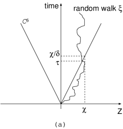
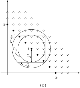
Figure 1: (a) Illustration of the space-time cone $C^{\delta}$ for $d=1$ and the definition of $\tau$ and $\chi$. (b) Illustration of the region of influence of site $i$ for $d=2$.

We are now ready to define the region of influence of a site. From now on we fix $k$ and $i\in J_{k}$, and we denote by $B_{i}$ the region of influence of site $i$. We couple $M_{i}$ and $N_{i}$ so that $M_{i}\geq N_{i}$. If $M_{i}=0$, we set $B_{i}=\emptyset$. Otherwise we proceed as follows. We construct a region for each of the $N_{i}$ particles that visit $K_{i}$. Consider the $j$th such particle and let $\chi_{j}$ be an independent random variable distributed as $\chi$, and define $t_{j}$ as the first time the particle visits $K_{i}$. With this, define the space-time cylinder

$$S_{j}=(B(i,\chi_{j})\cap\mathbb{H}_{d})\times[t_{j},t_{j}+\chi_{j}/\delta],$$

where $B(x,r)\subset\mathbb{Z}^{d}$ stands for the ball of radius $r$ centered at $x$. Note that, for any time $s\geq t_{j}+\chi_{j}/\delta$, the particle is inside the space-time cone $C_{i,t_{j}}^{\delta}$. Consequently, at any time $s\geq t_{j}+\chi_{j}/\delta$, the $j$th particle cannot intersect $\bigcup_{z\in\mathbb{H}_{d}}K_{z}$; hence the sites $\iota\in\mathbb{H}_{d}$ for which $j$ can intersect $K_{\iota}$ are contained in $S_{j}$. Define $\chi_{j}$ in the same way as above for all $N_{i}<j\leq M_{i}$, and take $L_{i}=\max_{j=1}^{M_{i}}\chi_{j}$ and $B_{i}=B(i,L_{i})\cap\mathbb{H}_{d}$. Note that $B_{i}$ contains all sites that intersect $\bigcup_{j=1}^{N_{i}}S_{j}$. Since the $\{M_{i}\}_{i\in J_{k}}$ are i.i.d. random variables, the regions $\{B_{i}\}_{i\in J_{k}}$ are also i.i.d.

We have the following lemma bounding the size of $B_{i}$.

Lemma 3.3.

There exist constants $c,c^{\prime}>0$ independent of $\lambda$ such that, for all $x\geq 1$ and $i\in\mathbb{H}_{d}$,

$$\operatorname{\mathbf{P}}\left(L_{i}>x\right)\leq c\lambda\exp(-c^{\prime}x).$$

Proof.

First we derive an upper bound for $\operatorname{\mathbf{P}}\left(\chi\geq x\right)$. The probability that a random walk performs at least $x$ jumps in a time interval of length $x/2$ is $e^{-c_{1}x}$ for some positive constant $c_{1}$. If this does not happen, then $\chi$ can only be at least $x$ if at some time after $x/2$ the random walk is outside the cone $C^{\delta}$. For any integer $a\geq 0$, let $I_{a}$ be the time interval $[z/2+a,z/2+a+1]$. We show that, during $I_{a}$, the probability that the distance between the random walk and the origin exceeds $\delta(x/2+a)$ is at most $e^{-c_{2}(x+a)}$ for some positive constant $c_{2}=c_{2}(d,{S})$. This follows since, with probability $1-e^{-c_{3}(x+a)}$, the random walk is within distance $\frac{\delta(x/2+a)}{2}$ from the origin at time $x/2+a$ and, with probability $1-e^{-c_{4}(x+a)}$, the random walk performs less than $\frac{\delta(x/2+a)}{2}$ jumps during a time interval of length $1$. Then, summing over $a$ we obtain

$$\operatorname{\mathbf{P}}\left(\chi\geq z\right)\leq c_{5}e^{-c_{6}z}\quad\text{for some positive constants $c_{5}=c_{5}(d,{S})$ and $c_{6}=c_{6}(d,{S})$.}$$

From this, we obtain

$$\operatorname{\mathbf{P}}\left(L_{i}>x\right)\leq\operatorname{\mathbf{E}}\left[M_{i}\right]\operatorname{\mathbf{P}}\left(\chi>x\right)\leq cc_{5}\lambda e^{-c_{6}x},$$

where $c$ comes from Lemma 3.2. ∎

Now we refer to Figure 1(b). If $B_{i}=\emptyset$, set $Q_{i}=\emptyset$. Otherwise, let $Q_{i}$ be the square $i+[-L_{i},L_{i}]^{d}\cap\mathbb{H}_{d}$ of side length $2L_{i}$; note that $B_{i}$ is inscribed inside $Q_{i}$. Consider the $2$-dimensional circle $B_{i}^{\prime}$ that circumscribe $Q_{i}$; the radius of $B_{i}^{\prime}$ is $\sqrt{2}L_{i}$. Now consider any site $\iota\in B_{i}$ so that $\iota\in J_{k^{\prime}}$ for some $k^{\prime}\geq k$, and take any oriented path from the origin to $\iota$. By construction, this path must contain a site in $Q_{i}\cap J_{k}$.

Now, for any $i\in\mathbb{H}_{d}$, we define $Y_{i}=0$ if there exists a $j\in\mathbb{H}_{d}$ with $\|j\|_{1}=\|i\|_{1}$ for which $i\in Q_{j}$. Otherwise, we set $Y_{i}=1$. From the argument above we have that we can couple $Y_{i}$ and $E_{i}$ so that $Y_{i}\leq E_{i}$. Therefore, if $\{Y_{i}\}_{i\in J_{k}}$ stochastically dominates $\{X_{i}\}_{i\in J_{k}}$ we establish (6). This last statement holds since the radius of $B_{i}^{\prime}$ has an exponential tail by Lemma 3.3. Also, the sites $i\in\mathbb{H}_{d}$ for which $\|i\|_{1}=k$ form a one-dimensional line segment, thus we can apply a result by Holroyd and Martin [2, Theorem 3], which establishes that $\{Y_{i}\}_{i\in J_{k}}$ stochastically dominates $\{X_{i}\}_{i\in J_{k}}$, where $\{X_{i}\}_{i\in J_{k}}$ are i.i.d. Bernoulli random variables with mean approaching $1$ as $\lambda\to 0$. This establishes (6) and completes the proof of Proposition 2.1.

4 Brownian motions on $\mathbb{R}^{d}$

In this section we discuss how the proof of Theorem 1.1 can be adapted to the setting where particles perform independent Brownian motions on $\mathbb{R}^{d}$, $d\geq 2$, and the target is detected as soon as it is within distance $1$ from any particle.

The main changes needed in the proof regards the definition of the space-time region $K_{i}$ and the definition of the region of influence $B_{i}$. We start with $K_{i}$. For all $i\in\mathbb{H}_{d}$, define $K_{i}=B(i,4/3)\times T_{i}$, where $B(i,r)$ is the $d$-dimensional closed ball on $\mathbb{R}^{d}$ of radius $r$ centered at $i$, and $T_{i}$ is defined as in (4). Then, the proof of Theorem 1.1 (assuming Proposition 2.1) carries through with no further changes, and it remains to show how the proof of Proposition 2.1 needs to be changed to this setting.

The proof of Proposition 2.1 is composed of three lemmas. Lemma 3.1 holds without any changes. For Lemma 3.2, the only change we need is to define $N_{i}$ as the number of particles of $\Psi_{k}$ that visit $B(i,4/3)$ during the interval $[k/{S},(k+1)/{S}]$, and first visit $B(i,4/3)$ not after visiting $B(j,4/3)$ for every $j\in J_{k}\setminus\{i\}$. (Note that we allow that the particle visits $B(i,4/3)$ concurrently to visiting $B(j,4/3)$ for some $j\in J_{k}\setminus\{i\}$; in this case, this particle counts to $N_{i}$ and an independent copy of the particle counts to $N_{j}$.) Then Lemma 3.2 follows in the same way.

For Lemma 3.3, we need to do more changes since we need to define $B_{i}$ and $L_{i}$ differently. From now on, fix $k$ and $i\in J_{k}$. Then let $x\in B(i,4/3)$ and $t\in T_{i}$ be arbitrary. We regard $x$ as the location and $t$ the time that the particle first visits $B(i,4/3)$. Consider the cone $C^{\delta}_{x,t}=(x,t)+C^{\delta}$. Then, for any $j\not\in B(i,5)$ and $s\in T_{j}$ we have

$$s-t\leq\frac{1+\|j\|_{1}-\|i\|_{1}}{{S}}\leq\frac{1+\|j-i\|_{2}}{4\delta}\leq\frac{1+4/3+\|j-x\|_{2}}{4\delta}\leq\frac{\|j-x\|_{2}}{2\delta},$$

where in the second to last step we apply the triangle inequality, and in the last step we used that $\|j-x\|_{2}\geq 3$ since $j\not\in B(i,5)$. Since, for any $(j,s^{\prime})\in C^{\delta}$, it holds that $s^{\prime}-t>\frac{\|j-x\|_{2}}{\delta}$, we obtain that $C^{\delta}$ does not intersect any $T_{j}$ for which $j\not\in B(i,5)$. Now let $\ell$ be a particle from the set of the $N_{i}$ particles that visit $B(i,4/3)$ during the interval $[k/{S},(k+1)/{S}]$, and do so before visiting $B(i^{\prime},4/3)$ for every $i^{\prime}\in J_{k}\setminus\{i\}$. Let $\chi_{\ell}$ be a random variable distributed as $\chi$ (cf (7)), and let $L_{i}$ be the maximum of $\chi_{\ell}$ over all $\ell$. Then, we set $B_{i}=B(i,10+L_{i})$ if $M_{i}\geq 1$. With these definitions, Lemma 3.3 holds without further changes and we obtain that the random variable $L_{i}$ has an exponential tail. Then, the remaining of the proof of Proposition 2.1 hold by setting $Q_{i}=i+[-10-L_{i},10+L_{i}]^{d}\cap\mathbb{H}_{d}$ and $B_{i}^{\prime}$ as the ball that circumscribe $Q_{i}$. No further change is needed.

References

- [1] A. Drewitz, J. Gärtner, A.F. Ramírez, and R. Sun. Survival probability of a random walk among a poisson system of moving traps. In Probability in Complex Physical Systems, Springer Proceedings in Mathematics, volume 11, pages 119–158. Springer-Verlag, 2012.
- [2] A.E. Holroyd and J. Martin. Stochastic domination and comb percolation, 2012. Preprint at arXiv:1201.6373.
- [3] G. Kesidis, T. Konstantopoulos, and S. Phoha. Surveillance coverage of sensor networks under a random mobility strategy. In Proceedings of the 2nd IEEE International Conference on Sensors, 2003.
- [4] H. Kesten and V. Sidoravicius. The spread of a rumor or infection in a moving population. The annals of probability, 33:2402–2462, 2005.
- [5] T. Konstantopoulos. Response to Prof. Baccelli’s lecture on modelling of wireless communication networks by stochastic geometry. Computer Journal Advance Access, 2009.
- [6] Y. Peres, A. Sinclair, P. Sousi, and A. Stauffer. Mobile geometric graphs: Detection, coverage and percolation. Probability Theory and Related Fields, 156:273–305, 2013.
- [7] Y. Peres and P. Sousi. An isoperimetric inequality for the Wiener sausage. Geometric and Functional Analysis, 22:1000–1014, 2012.
- [8] A. Stauffer. Space-time percolation and detection by mobile nodes, 2011. Preprint at arXiv:1108.6322v1.