Contributors of carbon dioxide in the atmosphere in Europe

Abstract.

Carbon dioxide, along with atmospheric temperature are interacting to cause what we have defined as global warming. In the present study we develop a statistical model using real data to identify the attributable variables (risk factors) that cause the CO₂ emissions in the atmosphere in Europe. Some scientists believe that there are more than nineteen attributable variables that cause the CO₂ in our atmosphere. However, our study has identified only three individual risk factors and five interactions among the attributable variables that cause almost all the CO₂ emissions in the atmosphere in Europe. We rank the risk factors and interactions according to the amount of CO₂ they generate. In addition, we compare the present findings of the Eupean data with a similar study for the Continental United States [1, 2]. For example, in the US, liquid fuels ranks number one, while in Europe is gas fuels. In fact, liquid fuels in Europe is the least contributable variable of CO₂ in the atmosphere, and gas fuels ranks seventh.

1. Introduction

The proposed model that we are developing takes into consideration individual contributions and interactions along with higher order contributions if applicable. In developing the statistical model, the response variable is the CO₂ in the atmosphere and is given in parts per million by volume (ppmv). In the present analysis, we used real yearly data that has been collected from 1959 to 2008 at Mauna Loa Observatory, Hawaii. The CO₂ emission data for the EU countries (list given below) was obtained from Carbon Dioxide Information Analysis Center (CDIAC) during the same period. The analysis presented here consists of two steps: first, we partially replicate the comprehensive study performed in [1, 2] in order to select the relevant variables and their interactions, and then we validate and analyze the best second-order model. Based on this result, we will perform the surface-response analysis (curvature effects) of the model in a forthcoming publication [3].

Figure 1. Schematic representation of the carbon cycle (DOE report [4] and supporting documentation).

The following 23 EU countries were used in this study: Austria, Belgium, Bulgaria, Cyprus, Czech Republic, Denmark, Finland, France, Germany, Greece, Hungary, Ireland, Italy, Luxembourg, Malta, Netherlands, Poland, Portugal, Romania, Slovakia, Spain, Sweden, United Kingdom.

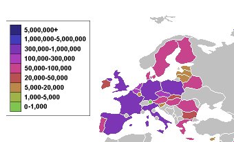
Figure 2. EU CO₂ emissions, in thousands of metric tons [7].

The aim of this study is two-fold: in the current paper we focus on the determination of the optimal second-order model (including interactions as well as quadratic terms) which provides the best fit for the data and features robust validation; in a forthcoming publication, we will use the model derived here in order to determine multi-variables confidence regions and obtain estimates for the allowed fluctuations in attributable variables, given a maximal range of change in the response variable. The second-order model we will obtain in the current study provides us with a list of relevant variables, ranked according to their statistical significance (quantified by the respective contribution to the total variability), which we employ in order to compare with the similar result obtained in the case of the U.S. data [1, 2].

2. Regression analysis and model building

One of the underlying assumptions to construct the model is that the response variable should follow Gaussian distribution. It is known [1, 2] that the CO₂ in the atmosphere does not follow the Gaussian distribution. Therefore, the Box-Cox transformation is applied to the CO₂ atmosphere data to filter the data to be normally distributed. After the Box-Cox filter, we retest the data and it shows our data will follow normal distribution; thus, we proceed to estimate the coefficients of the contributable variables for the transformed CO₂ atmosphere data. The parameter of the transformation is the same as the one used in the two previous studies [1, 2].

We can proceed to estimate the approximate coefficients of the contributable variables for transformed CO₂ in the atmosphere and obtain the coefficients of all possible interactions, using the multivariate regression procedure and corresponding goodness-of-fit measures.

We begin with seven attributable variables and apply the SAS stepwise forward selection procedure to a model with six relevant variables and 21 second-order interactions between each pair and self-interactions. Introducing the notation $x_{1}=$ Liquid Fuels (Li), $x_{2}=$ Gas Fuels (Ga), $x_{3}=$ Gas Flares (Fl), $x_{4}=$ Bunker (Bu) for the relevant attributable variables, we find that only three of the variables (Liquid Fuels ($x_{1}$), Gas Fuels ($x_{2}$), and Gas Flares ($x_{1}$)) and only 3 interactions (Ga:Bu, Li:Fl, Li:Bu) and two quadratic terms (Li², Bu²) are statistically relevant at $\alpha=0.01$ level.

The result of estimation becomes the quadratic model with interactions:

$$[\widehat{CO}_{2}]^{-2.376} = 0.00000123+(710.85Fl-30.64Ga-3.4501Li)\times 10^{-13}+$$

$$+ (37.34Ga\cdot Bu+1.35Li\cdot Li-65.12Bu\cdot Bu-$$

$$- 133.05Li\cdot Fl-5.35Li\cdot Bu)\times 10^{-18}.$$

The quality of the fit for this quadratic model is evidenced by high value of both $R^{2}$ and $R^{2}_{adjusted}$ which are the key criteria to evaluate the model fitting. In terms of the total ($SS_{t}$), regression ($SS_{r}$ and error ($SS_{e}$) sums of squares, we have the standard formulas

$$R^{2}=\frac{SS_{r}}{SS_{t}},\quad R^{2}_{adjusted}=1-\frac{SS_{e}/df_{e}}{SS_{t}/df_{t}},$$

with $df_{e,t}$ the degrees of freedom for the chi-squared distributions for error and total, respectively [5]. We also employ the prediction of residual error sum of squares ($PRESS$) statistics which will evaluate how good the estimation will be if each time we remove one data point. If the index $i$ covers all the observations and $\hat{y}_{(i)}$ is the predicted value when the observation is omitted, then [6]

$$PRESS=\sum_{i}\left(y_{i}-\hat{y}_{(i)}\right)^{2}.$$

Table 1. Statistical evaluation criteria for model (1)

$R^{2}$	$R^{2}_{{adjusted}}$	${PRESS}$
$0.9979$	$0.9975$	$1.636\times 10^{-20}$

According to these goodness-of-fit measures, the model we have obtained is high quality and reliable for predictions. The model becomes:

(1) $$[\widehat{CO}_{2}]^{-2.376}=\beta_{0}+\sum_{i=1}^{4}\beta_{i}x_{i}+\sum_{i\leq j=1}^{4}\beta_{ij}x_{i}x_{j},$$

with the corresponding ranks determined by the stepwise SAS procedure are given in Table 2, along with the coefficients in the final regression model.

Therefore, we can write our model in matrix notation (where prime denotes transposition) as:

(2) $$Y=\beta_{0}+\beta^{\prime}\cdot X+X^{\prime}\cdot B\cdot X,$$

with the obvious identifications

$$X^{\prime}=(x_{1},\ldots,x_{4}),\,\,\beta^{\prime}=(\beta_{1},\ldots,\beta_{4}),\,\,B_{ij}=B_{ji}=\frac{1}{2}\beta_{ij}\,\,(i<j).$$

Table 2. Ranking by statistical relevance for attributable variables and interactions.

Rank	Variable	Name	$\beta[\times 10^{-18}]$	Variation
$1$	Ga ($x_{2}$)	Gas Fuels	$-30.635\times 10^{5}$	$48.72\%$
$2$	Ga:Bu ($x_{2}\times x_{4}$)	Gas $\times$ Bunker	$37.3391$	$12.41\%$
$3$	Li2 ($x_{1}^{2}$)	Liquid $\times$ Liquid	$1.35565$	$11.79\%$
$4$	Bu2 ($x_{4}^{2}$)	Bunker	$-65.115$	$7.78\%$
$5$	Fl ($x_{3}$)	Gas Flares	$710.848\times 10^{5}$	$6.66\%$
$6$	Li:Fl ($x_{1}\times x_{3}$)	Liquid $\times$ Flares	$-133.05$	$5.06\%$
$7$	Li:Bu ($x_{1}\times x_{4}$)	Liquid $\times$ Bunker	$-5.3501$	$4.71\%$
$8$	Li ($x_{1}$)	Liquid Fuels	$-3.4501\times 10^{5}$	$2.86\%$

More precisely, the vector $\beta$ (up to an overall scale factor of $10^{-13}$), and the symmetric matrix $B$ (up to an overall scale factor of $10^{-18}$) have the forms:

$$\beta=\left[\begin{array}[]{c}-3.4501\\ -30.635\\ 710.848\\ 0\end{array}\right],\,B=\left[\begin{array}[]{cccccc}2.7113&0&-133.05&0\\ 0&0&0&37.3391\\ -133.05&0&0&0\\ 0&37.3391&0&-130.23\\ \end{array}\right]$$

These results will be used to perform the surface response analysis for the model, in a separate publication. The matrix formulation of the quadratic expression (1) will be the starting point for finding its canonical decomposition, based on the eigenvalue analysis [3].

2.1. Validation of the fitted model

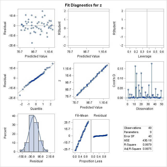
Figure 3. Residual plots and other fit diagnostics for the dependent variable (from the SAS output).

Based on the standard diagnostics provided by the SAS regression procedure, we can quantify the reliability and accuracy of the model (1). Specifically, the normalized predicted value for residuals (first panel in Figure 3), residual quantile plot, and the predicted value for the dependent variable, all indicate that the model is accurately describing the total variability in the data, and that the canonical normality assumptions are satisfied.

To further assess the robustness of (1), we employed multiple cross-validation by partitioning the full data set into smaller, equal-sized sets, and then fitting the model using all but one of the subsets. The predicted values for the missing observations (from the subset removed from the analysis) are then computed and quantified using their mean value and dispersion.

Specifically, we divided the data set into 49 data sets and use all 48 sets to construct the model and validate the model using the one left out. Then we repeat the procedure 48 times. The mean of the residuals is 5.427845e-22 and the variance of the residuals is 2.806e-44.

3. Comparing the US and EU models

Using the results obtained in [2], it is possible develop a comparison between the US and EU quadratic models for attributable variables and interactions; in particular, it is possible to compare the relative relevance of the main single-factor variables and of the main interactions (see Table 3 below and Table 3.4 from [1]).

Table 3. Comparison of statistical relevance for attributable variables and interactions, US vs. EU.

Rank	Variable in US	Variable in EU
$1$	Liquid	Gas
$2$	Liquid:Cement	Gas:Bunker
$3$	Cement:Bunker	Liquid:Liquid
$4$	Bunker	Bunker:Bunker
$5$	Cement	Gas Flares
$6$	Gas Flares	Liquid:Gas Flares
$7$	Gas	Liquid:Bunker
$8$	Gas:Gas Flares	Liquid

3.1. Specific features of CO₂ contributors for EU data

As Table 3 indicates, the most significant risk factor found when studying the US data (Liquid fuels) is the least relevant in the case of the EU data; likewise, the main attributable variable obtained for the EU data (Gas fuels) is the least relevant single-factor in the case of the US data (rank 7 out of 8). In view of the importance of the variable Gas fuel for the EU data, we indicate the individual contributions at country-level, for the year 2008, in Table 4.

This important difference between the rankings of risk factors for EU and US suggests two directions for further comparisons:

• for the purpose of CO₂ emission reductions, a very different picture emerges from the EU study versus the US study. Consider the information shown on Tables 2, 3, and 4: almost 50% of the total variability in the atmospheric CO₂ is due to Gas Fuels alone, which ranks first among the risk factors; furthermore, more than 25% of the total emissions for this factor is due to a single country, Germany (for year 2008).

• when developing criteria for trade-off of single risk factors (as in “cap-and-trade” schemes and beyond), specific information from each continent must be employed, as discussed in the next section. While this point further emphasizes the regional aspect of CO₂ analysis, it also illustrates the inherent limitations of applying carbon-accountability policies from one continent to another.

Table 4. Contributions by country to gas fuel emissions, for year 2008 (in thousand metric tons of carbon).

Rank	Country	Total	Percent
1	GERMANY	85457	27.19%
2	POLAND	58395	18.58%
3	UK	37306	11.87%
4	CZECH REP.	21021	6.69%
5	ITALY	16855	5.36%
6	SPAIN	14669	4.67%
7	FRANCE	13383	4.26%
8	ROMANIA	9805	3.12%
9	GREECE	8946	2.85%
10	BULGARIA	8058	2.56%
11	NETHERLANDS	7346	2.34%
12	FINLAND	5478	1.74%
13	BELGIUM	4361	1.39%
14	SLOVAKIA	4205	1.34%
15	DENMARK	4062	1.29%
16	AUSTRIA	3896	1.24%
17	HUNGARY	3275	1.04%
18	PORTUGAL	2644	0.84%
19	SWEDEN	2530	0.80%
20	IRELAND	2519	0.80%
21	LUXEMBOURG	86	0.03%
22	CYPRUS	29	0.01%
23	MALTA	0	0.00%

3.2. Regionalization of atmospheric CO₂ analysis

One relevant variable for the US market (Cement, together with its interactions to Liquid and Bunker) is completely absent in the case of the EU data. Together with the fact that, at the same level of statistical significance, the US model requires five variables while the EU data leads to a model with four, this shows that the two models are fundamentally different, in the sense that production, dynamics, and global interactions of the man-made factors responsible for atmospheric CO₂, are essentially different in the case of EU and UE.

This indicates that, when developing specific guidelines for industry regulations and accountability criteria, translating regulations and policies between the EU and US markets must be done with considerable caution. The differences found here mandate, in fact, that a specific approach must be developed in the EU case, and that adopting US-based policy directly may be unwarranted and outright misguided. We will quantify this aspect of the comparison in a forthcoming publication [3], aimed at comparing the possible carbon-production management in the case of the US versus the EU markets.

References

- [1] Yong Xu and Chris Tsokos (2013), Attributable variables with interactions that contribute to CO2 in the atmosphere, Frontiers in Science, 3(1): 6-13.
- [2] Chris Tsokos and Iuliana Teodorescu (2013), Surface response analysis and determination of confidence regions, preprint.
- [3] Chris Tsokos and Iuliana Teodorescu (2013), Contributors of carbon dioxide in the atmosphere in Europe: the surface response analysis, to be submitted.
- [4] US DOE. Climate Placemat: Energy-Climate Nexus, US Department of Energy Office of Science, 2008.
- [5] Ronald Christensen (2011), Plane answers to complex questions, Springer Texts in Statistics.
- [6] D. Allen (1974), The Relationship Between Variable Selection and Data Augmentation and a Method for Prediction, Technometrics, 16, 125-127.
- [7] http:en.wikipedia.org/wiki/File:Countries by carbon dioxide emissions world maps deobfuscated.png