Electron and Photon Identification
in the D0 Experiment

Abstract

The electron and photon reconstruction and identification algorithms used by the D0 Collaboration at the Fermilab Tevatron collider are described. The determination of the electron energy scale and resolution is presented. Studies of the performance of the electron and photon reconstruction and identification are summarized. The results are based on measurements of $Z$ boson decay events of $Z\to ee$ and $Z\to\gamma\ell\ell$ $(\ell=e,\mu)$ collected in $p\bar{p}$ collisions at a center-of-mass energy of 1.96 TeV using an integrated luminosity of up to 10 fb^-1.

I Introduction

The precise and efficient reconstruction and identification of electrons and photons at the D0 experiment at the Fermilab Tevatron $p\bar{p}$ collider is essential for a broad spectrum of physics analyses, including high precision standard model (SM) measurements and searches for new phenomena. To satisfy this requirement, the D0 detector was designed to have excellent performance for the measurements of electrons and photons of energies from a few GeV up to ${\cal{O}}$(100 GeV). Another design requirement was to have good discrimination between jets and electrons or photons, since physics measurements often suffer from large backgrounds induced by jets being misidentified as electrons or photons. In this paper, the reconstruction of electromagnetic (EM) objects using D0 data is described. The determination of the electron energy scale and resolution and the performance of electron and photon identification using the Run II dataset recorded between 2002 and 2011 are presented.

II D0 detector

The D0 detector is described elsewhere d0det . The components most relevant to electron and photon identification are the central tracking system, composed of a silicon microstrip tracker (SMT) that is located near the $p\bar{p}$ interaction point and a central fiber tracker (CFT) embedded in a 2 T solenoidal magnetic field, a central preshower (CPS), and a liquid-argon/uranium sampling calorimeter. The CPS is located before the inner layer of the calorimeter, outside the calorimeter cryostat, and is formed of one radiation length of absorber followed by three layers of scintillating strips. The D0 coordinate system is right-handed. The $z$-axis points in the direction of the Tevatron proton beam, and the $y$-axis points upwards. Pseudorapidity is defined as $\eta=-\ln[\tan(\theta/2)]$, where $\theta$ is the polar angle relative to the proton beam direction. The azimuthal angle $\phi$ is defined in the plane transverse to the proton beam direction. The SMT covers $|\eta|<3$, and the CFT provides complete coverage out to $|\eta|\approx 1.7$.

The calorimeter consists of a central section (CC) with coverage in pseudorapidity of $|\eta|<1.1$, and two endcap calorimeters (EC) covering up to $|\eta|\approx 4.2$, as shown in Fig. 1. The region $1.1<|\eta|<1.5$ is not fully covered by the calorimeter. Therefore, the reconstruction, identification, energy scale and resolution estimation methods described in the paper can not be used. In that particular region, the tracking system is mainly used for reconstruction which is beyond the scope of this paper. Each part of the calorimeter is contained in its own cryostat and comprises an EM section, closest to the interaction region, and a hadronic section. The EM section of the calorimeter is segmented into four longitudinal layers with transverse segmentation of $\Delta\eta\times\Delta\phi=0.1\times 0.1$, except in the third layer (EM3), where the segmentation is $0.05\times 0.05$. There are 32 azimuthal modules for EM layers in the CC. The hadronic section is composed of fine (FH) and coarse (CH) layers. The FH layers are closer to the interaction point, followed by the CH layers.

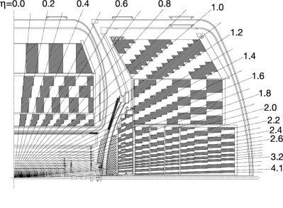
Figure 1: Side view of a quadrant of the D0 calorimeters showing the transverse and longitudinal segmentation. The alternating shading pattern indicates the cells for signal readout. The lines indicate the pseudorapidity intervals defined from the center of the detector. The CC covers the region $|\eta|<1.1$ and the EC extends the coverage to $|\eta|\approx 4.2$.

There is material varying between 3.4 and 5 radiation lengths ($X_{0}$) between the beam line and the CC. For EC, it varies between 1.8 and 4.8 $X_{0}$. The amount of material depends on the incident angle of the electron or photon MwPRD . At $\eta\approx 0$, the amount of material in front of the calorimeter is 0.2 $X_{0}$ in the tracking detector, 0.9 $X_{0}$ in the solenoid, 0.3 $X_{0}$ in the preshower detector plus 1.0 $X_{0}$ in the associated lead, and 1.3 $X_{0}$ in the cryostat walls plus related support structures.

III Data and Monte Carlo samples

Data and Monte Carlo (MC) simulated events have been used to study reconstruction and identification efficiencies, to measure the energy scale and resolution, and to derive correction factors to compensate for any residual mismodelling of the detector. The electron candidates are selected from $Z\to ee$ data and MC using the “tag-and-probe method” as described in Sect. VII.1. The photon candidates are selected from diphoton MC and $Z\to\gamma\ell\ell\ (\ell=e,\mu)$ data and MC, where the photons are radiated from charged leptons in $Z$ boson decays by requiring the dilepton invariant mass to be less than 82 GeV while the three-body mass of dilepton and photon $M_{\rm\ell\ell\gamma}$ is required to be $82<M_{\rm\ell\ell\gamma}<102$ GeV Zgam-ref . To evaluate misidentification of jets as electrons or photons, dijet events are selected. For dijet MC, an EM cluster passing the preselection as described in Sect. IV.1 is selected as jets misidentified as electrons or photons. For dijet data, a jet jesNIM with transverse momentum $p_{T}>20$ GeV and $|\eta|<2.5$ is selected, then a preselected EM cluster is selected in the opposite azimuthal plane with $|\Delta\phi(\rm jet,EM)|>2.9$ radian as the jets misidentified as electrons or photons. To eliminate possible contamination from diboson, $Z$ $+$ jets and $W$ $+$ jets processes, events with at least one isolated high-$p_{T}$ muon muonNIM , events with an invariant mass of the EM cluster and an isolated track between 60 and 120 GeV, and events with missing transverse energy MET-ref greater than 10 GeV are rejected. For studies of jets misidentified as photons, the $\gamma$ $+$ jet component containing a real photon is removed from the dijet sample by requiring that the EM cluster be non-isolated by cutting on the shower isolation fraction (see Sect. IV.1) of $0.07<f_{\rm iso}<0.15$. The $Z\to ee$ and $Z\to ee\gamma$ data events are collected using single electron triggers as described in Sect. VII.2. For $Z\to\mu\mu\gamma$ and dijet data events, single muon triggers muonNIM and jet triggers jesNIM are used, respectively.

The data used in physics analyses were collected by the D0 detector during Tevatron Run II between April 2002 and September 2011 and correspond to an integrated luminosity of approximately 10 fb^-1.

The $Z\to ee$ signal samples are generated using the alpgen generator alpgen-ref interfaced to pythia pythia-ref for parton showering and hadronization. The simulated transverse momentum $p_{T}$ distribution of the $Z$ boson is weighted to match the distribution observed in data zpt-ref . Diphoton and $Z\to\gamma\ell\ell\ (\ell=e,\mu)$ signal events, and dijet background samples are generated using pythia pythia-ref . All MC samples used here are generated using the CTEQ6L1 cteq-ref parton distribution functions, followed by a geant geant-ref simulation of the D0 detector. To accurately model the effects of multiple $p\bar{p}$ interactions in a single bunch crossing and detector noise, data from random $p\bar{p}$ bunch crossings are overlaid on the MC events. The instantaneous luminosity spectrum of these overlaid events is matched to that of the events used in the data analysis. Simulated events are processed using the same reconstruction code that is used for data.

IV EM object reconstruction and identification

EM objects – electrons and photons – are reconstructed by detecting localized energy deposits in the EM calorimeter. Confirmation of the existence of an electron track is sought from the central tracking system since an isolated high-$p_{T}$ track should originate from the interaction vertex. The hadronic calorimeter, preshower, and tracking systems can be used to differentiate electrons and photons from jets.

IV.1 EM cluster reconstruction

EM objects in the D0 detector are reconstructed using the nearly 55,000 calorimeter channels. Only channels with energies above noise are read out jesNIM . We use the same cluster reconstruction algorithm for electrons and photons, since their showers both consist of collimated clusters of energy deposited mainly in the EM layers of the calorimeter. Calorimeter cells with the same $\eta$ and $\phi$ are grouped together to form towers. For the calculation of the energy of EM clusters, we sum the energies measured in the four EM layers and the first hadronic (FH1) layer which is included to account for leakage of energy of EM objects into the hadronic part of the calorimeter. Starting with the highest transverse energy tower ($E_{T}>500$ MeV), energies of adjacent towers in a cone of radius ${\cal R}=\sqrt{(\Delta\eta)^{2}+(\Delta\phi)^{2}}=0.4$ around the highest $E_{T}$ tower are added to form EM clusters in the CC . In the EC, EM clusters are a set of adjacent cells with a transverse distance of less than 10 cm from an initial cell with the highest energy content in the EM3 layer.

To be selected as an EM candidate, EM clusters must satisfy the following set of criteria:

• The cluster transverse energy must be $E_{T}>$ 1.5 GeV.

• The fraction of energy in the EM layers is

  $$f_{\rm EM}=\frac{E_{\rm EM}}{E_{\rm tot}},$$ (1)

  where $E_{\rm EM}$ is the cluster energy in the EM layers, and $E_{\rm tot}$ is the total energy of the cluster in all layers within the cone. At least 90% of the energy should be deposited in the EM layers of the calorimeter.

• The isolation fraction is the ratio of the energy in an isolation cone surrounding an EM cluster to the energy of the EM cluster,

  $$f_{\rm iso}=\frac{E_{\rm tot}({\cal R}<0.4)-E_{\rm EM}({\cal R}<0.2)}{E_{\rm EM}({\cal R}<0.2)},$$ (2)

  where $E_{\rm tot}({\cal R}<0.4)$ is the total energy within a cone of radius ${\cal R}=0.4$ around the cluster, summed over the entire depth of the calorimeter except the CH layers, and $E_{\rm EM}({\cal R}<0.2)$ is the energy in the towers in a cone of radius ${\cal R}=0.2$ summed over the EM layers only. To select isolated electron or photon clusters in the calorimeter, we require an isolation fraction of less than 0.2.

For each EM candidate, the centroid of the EM cluster is computed by weighting cell coordinates with cell energies in the EM3 layer of the calorimeter. The shower centroid position together with the location of the $p\bar{p}$ collision vertex is used to calculate the direction of the EM object momentum.

Since EM objects begin to shower in the preshower detector, clusters are also formed in that detector. Single layer clusters are formed from scintillating strips for each layer. A preshower cluster is built by combining the single layer clusters from each of the three layers. These preshower clusters are extensively used to help identify the electrons and photons, and to build the multivariate identification methods, as well as to find the right interaction vertex for the photon as described in the following sections.

Electron candidates are distinguished from photon candidates by the presence of a track with $p_{T}>$ 1.5 GeV within a window of $\Delta\eta\times\Delta\phi=0.05\times 0.05$ around the coordinates of the EM cluster. The momentum of an electron candidate is recalculated using the direction of the best spatially matched track while the energy of the electron is measured by the calorimeter due to limited momentum resolution of the central tracking system. An EM cluster is considered to be a photon candidate if there is no associated track.

IV.2 EM object identification

After applying the above criteria to EM clusters, there remains a considerable fraction of jets misidentified as EM objects. Further criteria must be applied to reject these misidentified jets and increase the purity of the selected electron and photon candidates. The following is a description of the quantities employed for electron and photon identification. There are a number of different selection criteria for these quantities to meet the needs of different physics analyses.

EM energy fraction

Because the development of EM and hadronic showers are substantially different, shower shape information can be used to differentiate between electrons, photons, and hadrons. Electrons and photons deposit almost all their energy in the EM section of the calorimeter while hadrons are typically much more penetrating. EM clusters typically have a large EM fraction, $f_{\rm EM}$ (Eq. 1). The requirement of large values of $f_{\rm EM}$ is very efficient for rejecting hadrons, but also removes electrons pointing to the module boundaries (in $\phi$) of the central EM calorimeter, since they deposit a considerable fraction of their energy in the hadronic calorimeter.

EM shower isolation

Electrons and photons from a prompt decay of $W$ and $Z$ bosons tend to be isolated in the calorimeter, and therefore usually have a low isolation fraction $f_{\rm iso}$ (Eq. 2). In this case most of the energy of the EM cluster is deposited in a narrow cone of radius ${\cal R}=0.2$ in the calorimeter.

EM shower width

Showers induced by electrons and photons are usually narrower than those from jets. The EM3 layer of the calorimeter has a fine segmentation, providing sensitive variables to separate electrons and photons from misidentified jets. The squared width, $\sigma_{\phi}^{2}$, of the shower shape in the transverse plane is calculated as

$$\small\sigma_{\phi}^{2}=\frac{\sum(5.5+\log\left(\frac{E_{\rm cell}^{i}}{E_{\rm EM3}}\right))\cdot(r_{\rm cell}^{i}\times\sin(\phi_{\rm cell}^{i}-\phi_{\rm EM}))^{2}}{\sum(5.5+\log\left(\frac{E_{\rm cell}^{i}}{E_{\rm EM3}}\right))},$$ (3)

where $E_{\rm cell}^{i}$, $r_{\rm cell}^{i}$ and $\phi_{\rm cell}^{i}$ are the energy, radius calculated from $z$-axis and azimuthal angle for cell $i$ in the EM3 layer associated to the EM cluster, and $E_{\rm EM3}$ and $\phi_{\rm EM}$ are the total energy and centroid azimuthal angle of the EM cluster at the EM3 layer. A value of 5.5 was chosen as a result of studies to eliminate effect of low energy cells. Only the cells with positive weight $(5.5+\log\left(\frac{E_{\rm cell}^{i}}{E_{\rm EM3}}\right))>0$ are used in the calculation. The width $\sigma_{\eta}$ of the shower in the pseudorapidity direction is calculated as

$$\tiny\sigma_{\eta}=\sqrt{\frac{\sum(5.5+\log\left(\frac{E_{\rm cell}^{i}}{E_{\rm EM3}}\right))\cdot\eta_{i}^{2}}{\sum(5.5+\log\left(\frac{E_{\rm cell}^{i}}{E_{\rm EM3}}\right))}-\left(\frac{\sum(5.5+\log\left(\frac{E_{\rm cell}^{i}}{E_{\rm EM3}}\right))\cdot\eta_{i}}{\sum(5.5+\log\left(\frac{E_{\rm cell}^{i}}{E_{\rm EM3}}\right))}\right)^{2}},$$ (4)

where $E_{\rm cell}^{i}$ and $\eta_{i}$ are the energy and pseudorapidity of cell $i$.

H-matrix technique

The shower shape of an electron or a photon is distinct from that of a jet. Fluctuations cause the energy deposition to vary from the average in a correlated fashion among the cells and layers. Longitudinal and transverse shower shapes, and the correlations between energy depositions in the calorimeter cells are taken into account to obtain the best discrimination against hadrons, using a covariance matrix (“H-matrix”) technique hmatrix-1 ; hmatrix-2 . A covariance matrix is formed from a set of eight well-modeled variables describing shower shapes:

• The longitudinal development is described by the fractions of shower energy in the four EM layers (EM1, EM2, EM3, EM4).

• To characterize the lateral development of the shower, we consider the shower width in both dimensions in the third EM layer ($\sigma_{\phi}^{2}$ and $\sigma_{\eta}$), which is the layer with the finest granularity. The logarithm of the total shower energy and the coordinate of the $p\bar{p}$ collision vertex along the beam axis are included, so that the dependence of the H-matrix on these quantities is properly parametrized.

In the EC the matrix is of dimension $8\times 8$, while in the CC $\sigma_{\eta}$ is not used and therefore the matrix has the dimension $7\times 7$. A separate matrix is built for each ring of calorimeter cells with the same $|\eta|$ coordinate. To measure how closely the shower shape of an electron candidate matches expectations from MC simulations, a $\chi^{2}$ value is calculated ($\chi^{2}_{\rm Cal}$). Since the electron and photon candidates tend to have smaller $\chi^{2}_{\rm Cal}$ than jets, this variable can be used to discriminate between EM and hadronic showers.

Track isolation

For electrons and photons that are isolated, the scalar sum of the $p_{T}$ of all charged particle tracks with $p_{T}>0.5$ GeV, excluding the associated track for the EM cluster, originating from the $p\bar{p}$ collision vertex in an annular cone of $0.05<{\cal R}<0.4$ around the electron and photon candidates, $\Sigma p_{T}^{\rm trk}$, is expected to be small. It is therefore a sensitive variable for discriminating between EM objects and jets.

Track match

For electron identification, to suppress photons and jets misidentified as electrons, the cluster is required to be associated with a track in the central tracking system in a road between the EM calorimeter cluster and the $p\bar{p}$ collision vertex satisfying the conditions $|\Delta\eta_{\rm EM,trk}|<0.05$ and $|\Delta\phi_{\rm EM,trk}|<0.05$ for the differences between $\eta$ and $\phi$ of the EM cluster and the associated track. To quantify the quality of the cluster-track matching, a matching probability P($\chi^{2}_{\rm spatial}$) is defined using $\chi^{2}_{\rm spatial}$, which is given by

$$\chi^{2}_{\rm spatial}=\left(\frac{\Delta\phi}{\delta_{\phi}}\right)^{2}+\left(\frac{\Delta\eta}{\delta_{\eta}}\right)^{2}.$$ (5)

The probability is computed for each matched track. In these expressions, $\Delta\eta$ and $\Delta\phi$ are the differences between the track position and the EM cluster position in the EM3 layer of the calorimeter. The variables $\delta_{\phi}$ and $\delta_{\eta}$ are the resolutions of the associated quantities. The track with the highest P($\chi^{2}_{\rm spatial}$) is taken to be the track matched to the EM object. If there is no matched track, P($\chi^{2}_{\rm spatial}$) is set to $-1$.

Hits on road

Due to tracking inefficiencies, the cluster-track matching probability method is not fully efficient in separating electron from photon candidates, in particular in events with high instantaneous luminosity. To improve the separation between electron and photon candidates, a “hits on road” discriminant, $D_{\rm hor}$, is used in the CC. For each EM object, a “road” is defined between the $p\bar{p}$ collision vertex position and the CPS cluster position, if it is matched to the EM object, or else to the EM cluster position. To account for the different sign of the electric charge of electrons and positrons, two roads (positive-charge and negative-charge roads) are defined. The number of hits from CFT fibers and SMT strips along the EM cluster’s trajectory, $N_{\rm hits}$, is counted. The discriminant $D_{\rm hor}$ is defined by

$$D_{\rm hor}=\frac{P_{e}(N_{\rm hits})}{P_{e}(N_{\rm hits})+P_{\gamma}(N_{\rm hits})},$$ (6)

where $P_{e}$ and $P_{\gamma}$ are the probabilities in the bin of $N_{\rm hits}$, given by

$$P_{e}(N_{\rm hits})=\frac{\sum_{i=0}^{N_{\rm hits}}N_{e}^{i}}{\sum_{i=0}^{24}N_{e}^{i}},$$ (7)

$$P_{\gamma}(N_{\rm hits})=\frac{\sum_{i=N_{\rm hits}}^{24}N_{f}^{i}}{\sum_{i=0}^{24}N_{f}^{i}},$$ (8)

where $N_{e}^{i}$ and $N_{f}^{i}$ are the number of electrons and fake electrons in the bin $N_{\rm hits}=i$ from $Z\to ee$ and multijet data events, respectively. The maximum number of hits is 24, as the maximum of CFT hits is 16 and the maximum of SMT hits is 8. Electrons tend to have $D_{\rm hor}\approx 1$, while photons tend to have values close to 0.

Figs. 2-4 show distributions of identification variables for EM candidates from $Z\to ee$ data and MC events, as well as from diphoton and dijet MC events. As can be inferred from the distributions, the simulation has some imperfections in modeling the shower shapes mainly caused by an insufficient description of uninstrumented material MwPRD . This is accounted for when correcting simulated electron and photon identification efficiencies utilizing data as described in Sects. VII and VIII, respectively.

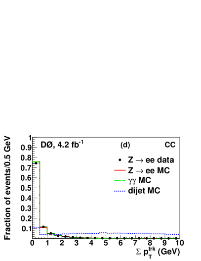
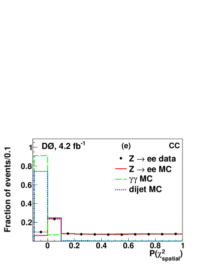
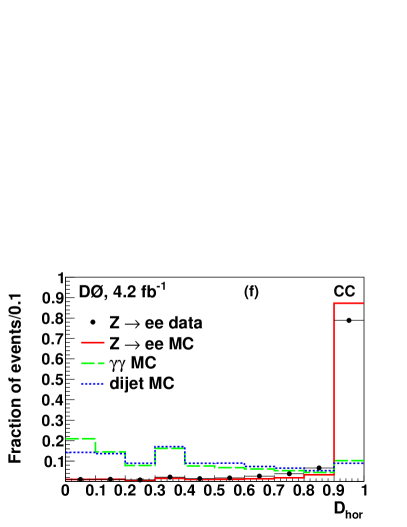
Figure 2: Normalized distributions of EM object identification variables as defined in Sect. IV.2 for $Z\to ee$ data and MC events, and for diphoton and dijet MC events in the CC. Presented are (a) the EM energy fraction, (b) the EM shower isolation, (c) the width of the EM shower in the transverse plane, (d) the track isolation, (e) the track matching probability, and (f) the hits on road discriminant. The first bin of the track matching probability distribution indicates no track match.

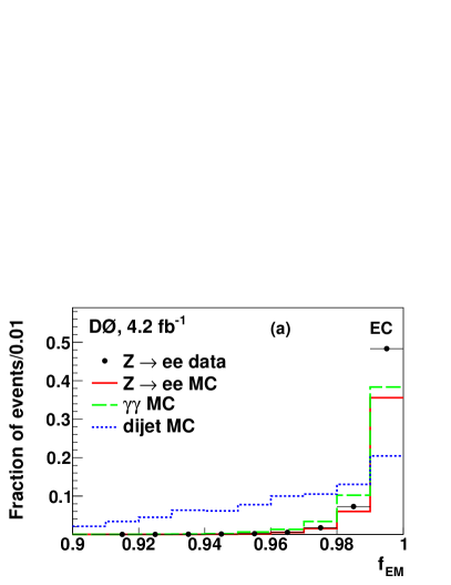
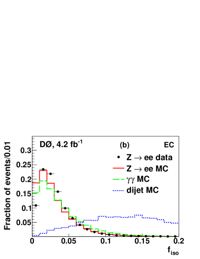
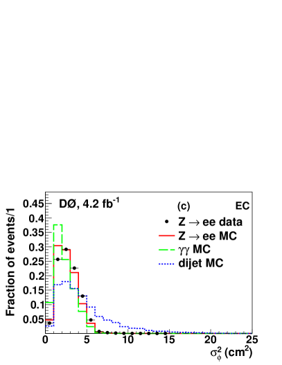
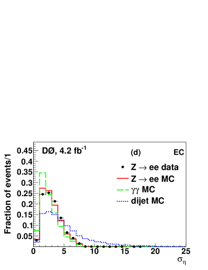
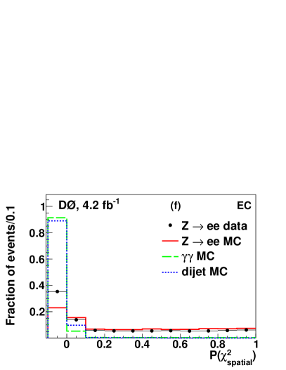
Figure 3: Normalized distributions of EM object identification variables as defined in Sect. IV.2 for $Z\to ee$ data and MC events, and for diphoton and dijet MC events in the EC. Presented are (a) the EM energy fraction, (b) the EM shower isolation, (c) the width of the EM shower in the transverse plane, (d) the width of the EM shower in the pseudorapidity direction, (e) the track isolation, and (f) the track matching probability. The first bin of the track matching probability distribution indicates no track match.

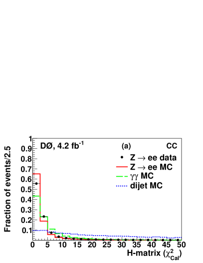
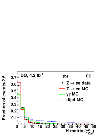
Figure 4: The distributions of $\chi^{2}_{\rm Cal}$ for EM candidates for $Z\to ee$ data and MC events, and for diphoton and dijet MC events in the CC (a) and EC (b).

V Multivariate identification methods

The variables described in Sect. IV.2 allow efficient identification of electron and photon candidates. However, to maximize the identification efficiencies of electrons and photons and to minimize the misidentification rate from jets in physics analyses, various multivariate analysis (MVA) techniques are explored. One MVA technique, the H-matrix method, has already been discussed in Sect. IV.2. Two more types of MVAs that are used in physics analyses are a Likelihood method for electrons and a neural network (NN) method for electrons and photons. H-matrix, Likelihood, and NN achieve an improved background rejection. However, the H-matrix is mainly based on the calorimeter information, while the Likelihood method includes the tracking information in addition, while the advantage of the NN is that it includes CPS information. The electron identification efficiency and purity are therefore found to be improved when these MVA output variables are utilized together with other electron reconstruction variables as input to a Boosted Decision Tree (BDT) BDT . All MVAs except the H-matrix are described in this section.

V.1 Electron Likelihood

Likelihood-based identification of electron candidates is an efficient technique for separating electrons from background by combining information from various detector components into a single discriminant.

There are several mechanisms by which particles, either isolated or in jets, may produce electron signatures. Photon conversions may be marked by the presence of a track very close to the track matched to the EM cluster, or a large $E_{T}/p_{T}$ when the closely situated $ee$ pair is reconstructed as a single EM cluster and only one track is identified. Here, $E_{T}$ is the transverse energy of the cluster measured by the calorimeter and $p_{T}$ is the transverse momentum of the associated track measured by the tracker. The calorimeter quantities describing the shower shape, however, are nearly identical to that of an electron, though photon calorimeter clusters may be slightly wider than an electron shower. Neutral pions $(\pi^{0})$ may also have nearby tracks, as they are generally produced in association with other charged hadrons. Since the $\pi^{0}\to\gamma\gamma$ decay would have to overlap with a charged hadron track in order to fake an electron, the track matching quantity could be poor, and the track would not necessarily be isolated. The H-matrix $\chi^{2}_{\rm Cal}$ and $f_{\rm EM}$ of the EM object may be influenced by the surrounding hadrons. The following eight variables are used to calculate the electron likelihood:

• EM energy fraction $f_{\rm EM}$;

• EM shower isolation $f_{\rm iso}$;

• H-matrix $\chi^{2}_{\rm Cal}$;

• $E_{T}/p_{T}$;

• transverse impact parameter of the selected track with respect to the $p\bar{p}$ collision vertex;

• number of tracks with $p_{T}>0.5$ GeV in a cone of radius ${\cal R}=0.4$ around and including the matched track;

• cluster-track matching probability P($\chi^{2}_{\rm spatial}$);

• track isolation variable $\Sigma p_{T}^{\rm trk}$.

The distributions of these eight variables are normalized to unit area to generate probability density distributions for each variable from $Z\to ee$ and dijet data for signal and background, respectively. These distributions are used to assign a probability for a given EM object to be signal or background. To quantify the degree of correlation between the input variables, we calculate the correlation coefficients. We find that most of the combinations have correlation coefficients close to zero and hence are mutually uncorrelated. Others do not exceed 55% for signal or fake electrons. The product of individual probabilities from all variables is correlated with the overall probability for the EM object to be an electron. To differentiate between signal-like and background-like electron candidates, a likelihood discriminant is calculated:

$$\mathcal{L}=\frac{P_{\rm sig}}{P_{\rm sig}+P_{\rm bkg}},$$ (9)

where $P_{\rm sig}$ and $P_{\rm bkg}$ are the overall probabilities for signal and background, respectively. Distributions of this discriminant for electron candidates in the CC and EC are presented in Fig. 5. This demonstrates the enhanced power to separate between genuine electrons, which peak at large values of the discriminant, and jets, which peak at low values.

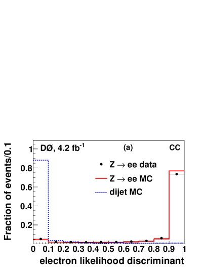
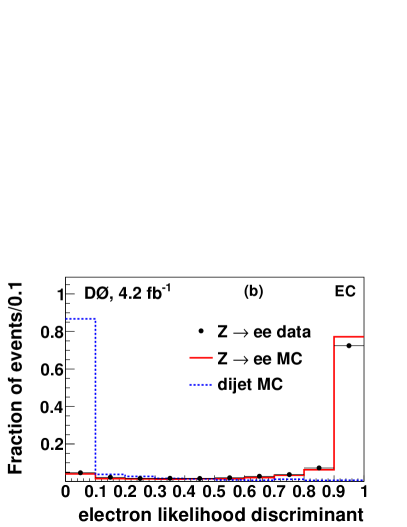
Figure 5: Distribution of the electron likelihood discriminant of electron candidates in $Z\to ee$ data and MC events, and in dijet MC events in the CC (a) and EC (b).

V.2 Neural Network for electron and photon identification

To further suppress jets misidentified as electrons and photons, we train an NN NN using a set of variables that are sensitive to differences between electrons (photons) and jets. The variables, selected to explore both the tracker activity and the energy distribution in the calorimeter and CPS, are listed below.

• fraction of the EM cluster energy deposited in the first EM calorimeter layer ($f_{\rm EM1}$);

• number of cells above an EM cluster $E_{T}$-dependent threshold, given by $0.004\times E_{T}$ (in GeV) $+$ 0.25 GeV in the first EM calorimeter layer within ${\cal R}<0.2$ ($N_{\rm cells}^{{\cal R}<0.2}$) and $0.2<{\cal R}<0.4$ ($N_{\rm cells}^{0.2<{\cal R}<0.4}$) of the EM cluster;

• track isolation variable $\Sigma p_{T}^{trk}$;

• number of charged particle tracks with $p_{T}>0.5$ GeV originating from the $p\bar{p}$ collision vertex within ${\cal R}<0.05$ of the EM cluster ($N_{\rm trks}^{{\cal R}<0.05}$);

• number of CPS clusters within ${\cal R}<0.1$ of the EM cluster ($N_{\rm cps}$);

• squared width of the energy deposit in the CPS:

  $$\sigma_{\rm CPS}^{2}=\frac{\sum_{i}E_{i}^{2}\times(\phi_{\rm EM}-\phi_{i})^{2}}{\sum_{i}E^{2}_{i}},$$ (10)

  where $E_{i}$ and $\phi_{i}$ are the energy and azimuthal angle of the $i^{th}$ strip in CPS in the direction of the EM cluster and $\phi_{\rm EM}$ is the azimuthal angle of the EM cluster at the EM3 layer;

• $\chi^{2}_{\rm Cal}$ calculated from the H-matrix.

Separate NNs are built for electrons and photons in the CC, whereas a single NN is used for electrons and photons in the EC. Table 1 lists the input variables utilized in each NN.

For the construction of the NN for electrons in the CC, the seven variables above are used as inputs ($e$NN7). Here, $Z\to ee$ data events define the signal, and dijet data events define the background. Performance checks have been performed using $Z\to ee$ and dijet MC events.

The NN for CC photons ($\gamma$NN5) is built from the same variables as $e$NN7 but excluding the tracker-based variable $N_{\rm trks}^{{\cal R}<0.05}$, and $f_{\rm EM1}$ since its distribution varies significantly with the $E_{T}$ of the EM cluster. The direct diphoton MC defines the signal, and dijet MC events are used as background in training the NN. For testing, the reconstructed radiated photon from $Z\to\ell\ell\gamma$ ($\ell=e,\mu$) events in data and MC events, and dijet MC events are used.

A photon NN ($\gamma$NN4) is built with four input variables as listed in Table 1 for the EC region. The training is based on direct diphoton and dijet MC events. The same types of events used to test $\gamma$NN5 are used to test $\gamma$NN4. Considering the similar performance of the input variables of electrons and photons in the EC, $\gamma$NN4 is found to work well, and is used, for electron identification in the EC.

Figure 6 shows the NN output distributions for reconstructed EM clusters with P($\chi^{2}_{\rm spatial}$) $>$ 0.001 (electron candidates) and without track match (photon candidates) for $Z\to ee$ data and MC events, and for dijet background MC events. The distributions show good agreement between data and MC simulation and demonstrate good separation between signal and background.

To validate the photon NNs for jets, dijet data events in the jet-enriched calorimeter isolation region $0.07<f_{\rm iso}<0.15$ are compared to MC simulation. As shown in Fig. 7, good agreement between data and MC is observed.

Input variables	$e$NN7 in CC	$\gamma$NN5 in CC	$\gamma$NN4 in EC
$f_{\rm EM1}$	$\surd$	$-$	$-$
$N_{\rm cells}^{{\cal R}<0.2}$	$\surd$	$\surd$	$\surd$
$N_{\rm cells}^{0.2<{\cal R}<0.4}$	$\surd$	$\surd$	$\surd$
$\Sigma p_{T}^{\rm trk}$	$\surd$	$\surd$	$\surd$
$N_{\rm trks}^{{\cal R}<0.05}$	$\surd$	$-$	$-$
$N_{\rm cps}$	$\surd$	$\surd$	$-$
$\sigma_{\rm CPS}^{2}$	$\surd$	$\surd$	$-$
H-matrix $\chi^{2}_{\rm Cal}$	$-$	$-$	$\surd$

Table 1: Input variables used in the NNs for electrons and photons in the CC and EC. For electrons in the EC, $\gamma$NN4 is used.

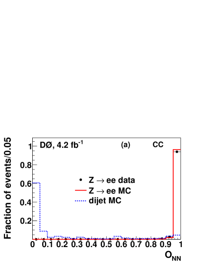
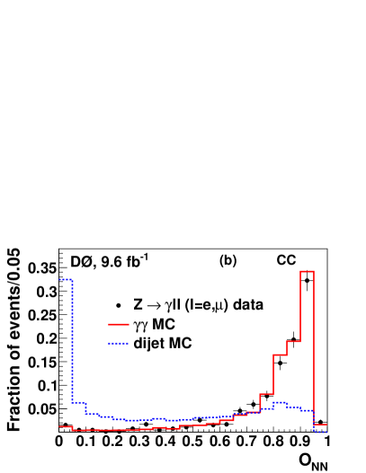
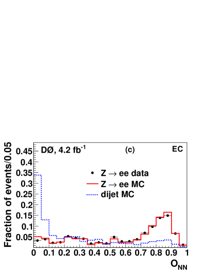
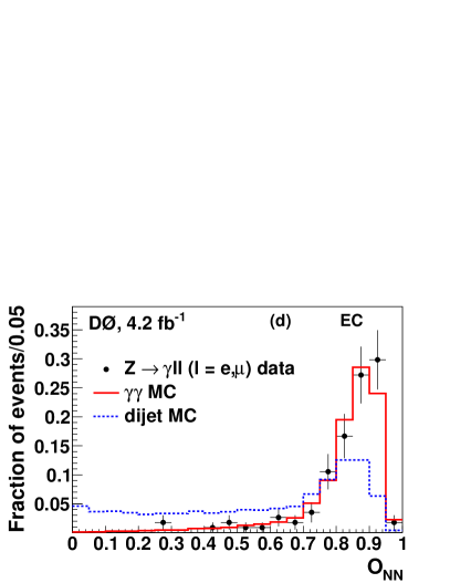
Figure 6: The output distributions of eNN7 for CC electrons (a), $\gamma$NN5 for CC photons (b), $\gamma$NN4 for EC electrons (c) and EC photons (d).

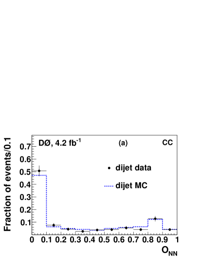
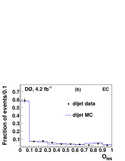
Figure 7: The output distributions of $\gamma$NN5 in CC (a) and $\gamma$NN4 in EC (b) for jet-like EM cluster candidates from dijet data and MC events.

V.3 Boosted Decision Trees for electron identification

To enhance the efficiency and purity in electron identification, a BDT is constructed utilizing variables that are significantly different for signal and background leading to a strong discrimination power of the BDT output distribution. The following variables are used to construct the BDT:

• EM energy fraction $f_{\rm EM}$;

• EM shower isolation $f_{\rm iso}$;

• energy fraction in EM1, EM2, EM3, EM4 and FH1;

• $\sigma_{\phi}^{2}$ in EM1, EM2, EM3, EM4 and FH1;

• $\sigma_{\eta}$ in EM1, EM2, EM3, EM4 and FH1;

• H-matrix $\chi^{2}_{\rm Cal}$;

• $\Sigma p_{T}^{\rm trk}$;

• cluster-track matching probability P($\chi^{2}_{\rm spatial}$);

• “hits on road” discriminant $D_{\rm hor}$ in CC;

• ratio $E_{T}/p_{T}$;

• number of hits from CFT fibers $N_{\rm CFT}$;

• number of hits from SMT strips $N_{\rm SMT}$;

• ratio $N_{\rm CFT}/N_{\rm SMT}$;

• number of hits in the first layer of the SMT;

• number of charged particle tracks with $p_{T}>0.5$ GeV originating from the $p\bar{p}$ collision vertex within ${\cal R}<0.05$ of the EM cluster;

• electron likelihood discriminant $\mathcal{L}$;

• output distribution of $e$NN7 in CC;

• output distribution of $\gamma$NN4 in EC;

• squared width of the energy deposit in the CPS $\sigma^{2}_{\rm CPS}$ in CC;

• $\chi^{2}$ for matching the spatial positions between CPS cluster and EM cluster in CC.

For the training of the BDT $Z\to ee$ and dijet data are used. The BDT is trained separately for the CC and EC and for high ($\mathcal{L}_{\rm inst}$ $>1.6\times 10^{32}$ cm^-2s^-1) and low instantaneous luminosities ($\mathcal{L}_{\rm inst}$ $<1.6\times 10^{32}$ cm^-2s^-1) leading to a different ranking of the utilized input variables. The training of separate BDTs for CC and EC is of advantage since the signal-to-background ratio is different in the two calorimeter regions, and the CC has a better coverage by the tracking devices. Similarly, differences in the signal-to-background ratio and in the resolution of various variables motivate the training of separate BDTs for high and low instantaneous luminosities.

The BDT output distributions are shown combined for all instantaneous luminosities but separately for CC and EC in Fig. 8. They represent the most powerful identification variables among the methods presented here. Typically, the signal efficiency is increased by 4%–8% while maintaining a similar fake rate as other methods. Due to the insufficient description of uninstrumented material in the MC simulation, discrepancy between data and MC exists. This has been studied and taken into account by applying corrections to the simulation.

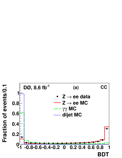
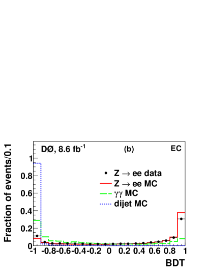
Figure 8: BDT output distributions of electron candidates in the CC (a) and EC (b) region for $Z\to ee$ data and MC events, and for dijet and diphoton MC events.

VI Energy scale and resolution calibration

After EM objects are identified as described in Sects. IV and V, the detector response to the energy of electrons and photons is calibrated. The electron energy scale and resolution are determined from $Z\to ee$ data events. EM showers induced by electrons and photons have similar distributions in the D0 calorimeter. However, EM clusters deposit energy in the passive material such as the inner detector and solenoid before reaching the calorimeter. On average, electrons lose more energy in this material than photons em-calorimeter . To account for this difference, MC simulations tuned to reproduce the response for electrons in data are used to derive the response difference between electrons and photons. In this section, the electron energy scale and resolution, and the energy scale difference between electrons and photons, are described.

VI.1 Energy scale

The amount of material in front of the calorimeter varies between 3.4 and 5 $X_{0}$ in the CC and between 1.8 and 4.8 $X_{0}$ in the EC MwPRD . The fraction of energy deposited in each longitudinal layer of the calorimeter depends on the amount of that passive material. The energy loss in passive material is studied taking into account the energy profile dependence on the incident angle rafael-thesis . The differences of the energy response between data and the MC simulation are determined using $Z\to ee$ events and the corrections are applied to the MC simulation.

The energy response is degraded near the module $\phi$ boundaries for the EM layers of the CC. In addition to a degradation of energy response, the centroid position of the EM cluster is shifted. To study these effects, the following variable is defined:

$$\mbox{$\phi_{\rm mod}$}\ ={\rm mod}\left(\frac{16\cdot\phi_{\rm EM}}{\pi},1\right),$$ (11)

where $\phi_{\rm EM}$ is the azimuthal angle of the EM cluster. For track-matched electrons, $\phi_{\rm mod}$ is determined by extrapolating the associated track through the known magnetic field towards the calorimeter. For photons and non-track-matched electrons, an average correction of the $\phi_{\rm mod}$ is applied which was determined from track-matched electrons. Regions of 0.1 $<$ $\phi_{\rm mod}$ $<$ 0.9 are referred to as “in-fiducial”, the values outside this range are defined as “non-fiducial”. Figure 9 shows the dielectron invariant mass ($M_{ee}$) distribution for $Z\to ee$ data events with two CC electrons. The distribution is shown separately for events with 0, 1, and 2 electrons located in fiducial regions. Electrons in or close to module boundaries suffer significant energy losses. To correct for such energy loss, the $\phi_{\rm mod}$ dependent energy scale corrections are derived for both data and MC simulation using $Z\to ee$ events. Due to the different amount of material traversed by the electrons before reaching the calorimeter, the events are split into five $\eta$ regions to derive the correction parameters. In addition, the energy loss near $\phi$ boundaries is larger for electrons with a poorly measured shower shape corresponding to a large H-matrix $\chi^{2}_{\rm Cal}$. The energy scale corrections are therefore derived as a function of $\phi_{\rm mod}$ and H-matrix $\chi^{2}_{\rm Cal}$.

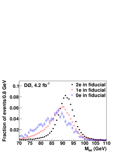
Figure 9: The $M_{ee}$ distribution in a sample of $Z\to ee$ data events, where both electrons are in the CC, and separating events with 0, 1 and 2 fiducial electrons. All three distributions are normalized to unit area.

With increasing $\mathcal{L}_{\rm inst}$ during Run II, the uncalibrated $Z$ boson mass is shifted to lower values in data events. The cause of this effect is discussed in Ref. MwPRD . The MC simulation, however, predicts an increase in the average EM energy with $\mathcal{L}_{\rm inst}$ due to extra energy from additional $p\bar{p}$ interactions. In the data, calibration of the calorimeter largely corrects for this energy scale dependence on $\mathcal{L}_{\rm inst}$. Residual offline corrections are derived by fitting the distribution of $E_{T}/p_{T}$ for electrons in $W\rightarrow e\nu$ events, taking advantage of the fact that the $p_{T}$ scale is independent of $\mathcal{L}_{\rm inst}$.

Individual cells in the EM calorimeter are known to saturate at energies varying from about 60 to 260 GeV, depending on the cell position. As a result, an EM cluster loses on average about 0.5% (6%) of its nominal energy at 300 (500) GeV. A simple correction truncates the energy of any cells in the MC that exceed the saturation value for that cell.

Due to the different amount of energy loss between electrons and photons in the passive material, the photon energy is over-corrected by applying the electron energy scale correction. The correction is about 3% at $p_{T}=20$ GeV, and it decreases at higher energies. The correction required for forward photons is slightly smaller. The reconstructed photon energy is corrected accordingly to compensate for the over-correction.

The systematic uncertainty for the electron energy scale correction is $\approx$0.5%, which is mainly caused by the limited statistics of $Z\to ee$ data events. For photons, additional 0.5% systematic uncertainty is added in quadrature from electron-to-photon energy scale correction.

VI.2 Energy resolution

The energy resolution of the calorimeter as a function of the electron/photon energy, E, can be written as

$$\frac{\sigma_{\rm EM}}{E}=\sqrt{C^{2}_{\rm EM}+\frac{S^{2}_{\rm EM}}{E}+\frac{N^{2}_{\rm EM}}{E^{2}}}$$ (12)

with $C_{\rm EM}$, $S_{\rm EM}$ and $N_{\rm EM}$ as the constant, sampling and noise terms, respectively. The constant term accounts for the non-uniformity of the calorimeter response. Its effect on the fractional resolution is independent of the energy, and therefore it is the dominant effect at high energies. The sampling term is due to the fluctuations related to the physical development of the shower, especially in sampling calorimeters where the energy deposited in the active medium fluctuates event by event because the active layers are interleaved with absorber layers. The noise term comes from the electronic noise of the readout system, radioactivity from the Uranium, and underlying events. Since the noise contribution is proportional to 1/E it is basically negligible for high energy electrons/photons. Due to the large amount of material in front of the calorimeter, $S_{\rm EM}$ is not a constant and is parametrized as a function of electron energy and incident angle MwPRD . The constant term $C_{\rm EM}$ is derived by a fit to the measured width of the $Z\to ee$ peak MwPRD . These terms are measured and applied to the true energy of electron for the fast simulation.

The electron and photon energy resolution predicted by the geant-based geant-ref simulation of the D0 detector is better than observed in data. Furthermore, there are non-Gaussian tails in the resolution distribution that are poorly modeled by the fully simulated MC described in Sect. III, partly because the finite charge collection time of the readout system of the calorimeter is neglected in the simulation. To account for both effects, an ad-hoc smearing is applied to the reconstructed energy of EM clusters following the geant simulation according to the following function, which was introduced by the Crystal Ball Collaboration crystalball-ref :

$$\tiny f(x;\alpha,n,\bar{x},\sigma)=\begin{cases}\exp(-\frac{(x-\bar{x})^{2}}{2\sigma^{2}}),&\text{for }\frac{x-\bar{x}}{\sigma}>-\alpha\\ (\frac{n}{\alpha})^{n}\exp(-\frac{\alpha^{2}}{2})(\frac{n}{\alpha}-\alpha-\frac{x-\bar{x}}{\sigma})^{-n},&\text{for }\frac{x-\bar{x}}{\sigma}\leq-\alpha\\ \end{cases}$$ (13)

Here, the $\sigma$ parameter determines the width of the Gaussian core part of the resolution. The $\alpha$ parameter controls the energy below which the power law is used, and the $n$ parameter governs the exponent of the power law. The $\bar{x}$ parameter is the mean of the Gaussian core part of the resolution. Typically, an increase in the width of the non-Gaussian tail needs to be compensated by an increase in the mean. The mean of $f(x)$ is around 0, and the simulated energy is scaled by $1+x$, where $x$ is sampled from the probability distribution function according to Eq. 13.

To determine the parameters of Eq. 13, a fit is performed by varying parameters applied to the MC, and minimizing the $\chi^{2}$ between the data and fully simulated MC in the $M_{ee}$ distribution. The $n$ parameter is fixed since there is enough freedom in the other three parameters to adequately describe the data. A value of $n=7$ is found to be appropriate.

The parameters are fitted separately for the following three categories of EM clusters mika-thesis :

• Category 1: CC in-fiducial
  CC in-fiducial clusters are defined as $|\eta|<1.1$ and 0.1 $<$ $\phi_{\rm mod}$ $<$ 0.9. The parameters are fitted using events in which both electrons are CC in-fiducial.

• Category 2: CC non-fiducial
  CC non-fiducial clusters are defined as $|\eta|<1.1$ and $\phi_{\rm mod}$ $<$ 0.1 or $\phi_{\rm mod}$ $>$ 0.9. The parameters are fitted using events containing two CC electrons, where at least one is non-fiducial. Any CC in-fiducial electrons are smeared using their already tuned parameters.

• Category 3: EC
  EC clusters are defined as having $|\eta|>1.5$. The parameters are fitted using events containing two EC electrons, or one CC in-fiducial or non-fiducial plus one EC electron. For EC clusters, a simple Gaussian smearing is used where the fit has only two parameters ($\bar{x}$, $\sigma$).

Figure 10 shows a comparison of $M_{ee}$ distributions for $Z\to ee$ data and MC after applying the energy scale and smearing corrections. Good agreement between data and MC simulation is observed.

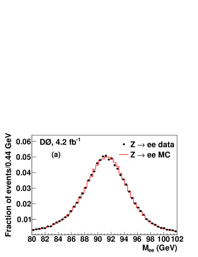
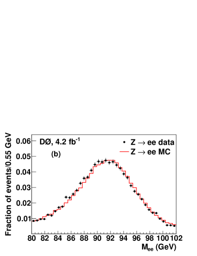
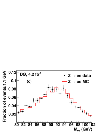
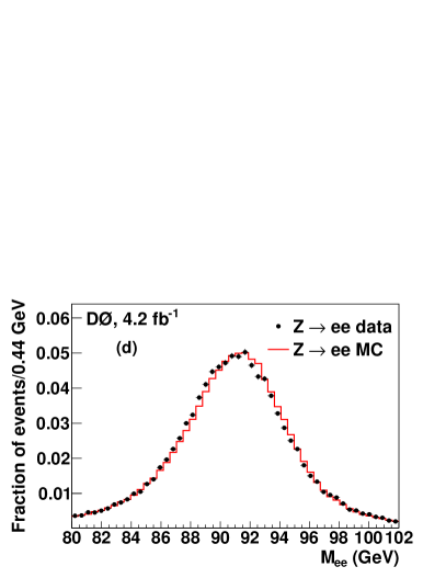
Figure 10: Dielectron invariant mass ($M_{ee}$) distributions for $Z\to ee$ data and MC events, with two electrons in the CC fiducial regions (a), one electron in the CC fiducial region and the other in the CC non-fiducial region (b), two electrons in the CC non-fiducial regions (c), and at least one electron in the EC region (d).

VII Efficiencies of electron identification

Electron trigger, preselection and identification efficiencies are measured in $Z\to ee$ data and MC events by selecting two high-$E_{T}$ electron candidates that have an invariant mass close to the $Z$ boson mass peak. To obtain an improved simulation, differences between the efficiencies measured in data and MC simulation are used to derive correction factors to be applied to MC events taking into account kinematic dependences.

VII.1 Tag-and-probe method

To measure the efficiencies, a “tag-and-probe method” is used. In $Z\to ee$ decays, a $E_{T}>30$ GeV electron candidate in CC fiducial is selected as the “tag” with the following requirements:

• $f_{\rm EM}>0.96$;

• $f_{\rm iso}<0.07$;

• $\Sigma p_{T}^{\rm trk}<2$ GeV;

• associated track $p_{T}>15$ GeV;

• $\mathcal{L}>0.8$;

• $e$NN7 $>$ 0.7.

The “probe” – used to perform the measurement of the identification efficiency – is either an EM cluster or a track. The invariant mass of the tag and probe electrons, $M_{tp}$, is required to be close to the $Z$ boson mass. If the probe is an EM cluster, $M_{tp}$ is required to be greater than 80 GeV but less than 100 GeV. The energy resolution for high-$p_{T}$ tracks is worse, and the $M_{tp}$ is required to be greater than 70 GeV but less than 110 GeV when the probe is a track. If the probe passes the tag selection criteria, it will also be used as a tag, resulting in the event being counted twice. To avoid bias, the same tag-and-probe method is used for both $Z\to ee$ data and MC events.

To remove the residual background from jet production in data events, a template fit is applied to the $M_{tp}$ distributions. The signal shape is obtained from $Z\to ee$ MC simulation, and the background shape is derived from dijet data. To take into account dependencies on the electron position in the detector, the template fit is performed in various $\eta$ and $\phi$ regions. The systematic uncertainty for the tag-and-probe method is dominated by the statistics of $Z\to ee$ data events. It is $\approx$10% for low probe $E_{T}$ ($<$ 20 GeV) region, and $\approx$3% for high probe $E_{T}$ region.

VII.2 Trigger efficiencies

There are two types of single electron triggers MwPRD ; trigger-ref . One class of triggers is solely based on calorimeter information and the other class includes tracking information. Calorimeter-based triggers are used for both electrons and photons. To have higher trigger efficiencies for electrons, we combine both types of triggers by taking their logical OR. The tag-and-probe method is used to measure the trigger efficiencies in data. To be consistent with offline electron identification requirements (described in Sect. VII.4), the trigger efficiencies are measured with respect to each set of electron identification requirements. To account for dependencies on the EM cluster position in the detector, the trigger efficiencies are parametrized as a function of $E_{T}$ and $\eta$ of the electron candidate. Single electrons are triggered with an efficiency $\approx$100% for transverse momenta above 30 GeV in the fiducial regions of the calorimeter up to $|\eta|<2.5$.

VII.3 Preselection efficiencies

Preselected electrons and photons are EM clusters that satisfy the criteria described in Sect. IV.1. The preselection efficiency is given by the fraction of tracks that match an EM cluster passing the preselection requirements for the probe electron candidate. In Fig. 11a the preselection efficiencies are presented for probe tracks in the CC as a function of $\phi_{\rm mod}$ for data and the MC simulation. The average efficiency is $\approx 98\%$. Data and MC simulation show good agreement, except in non-fiducial regions. Therefore, the $\phi_{\rm mod}$-dependent correction factors as shown in Fig. 11a are applied to MC to improve the simulation. Figure 11b shows the preselection efficiencies as a function of $\eta$ for EC electrons. Efficiency losses are observed in the region $|\eta|>2.5$ due to partial detector coverage for increasing $\eta$. To correct for data versus MC differences in the EC region, $\eta$-dependent factors are applied to the simulation. No significant differences between data and MC in other variables are observed for either electrons or photons in the CC and EC regions.

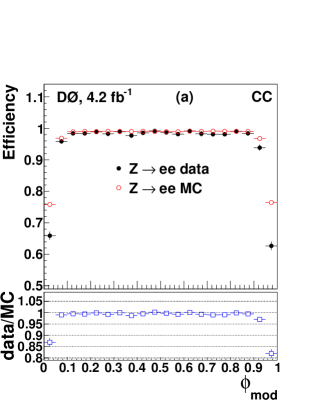
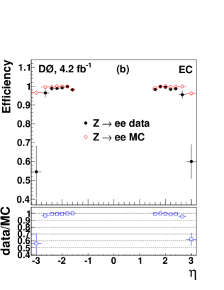
Figure 11: Preselection efficiencies of probe tracks as a function of $\phi_{\rm mod}$ and $\eta$ for electrons in the CC (a) and EC (b). $Z\to ee$ data is compared to the MC prediction, and the ratio data/MC is presented.

VII.4 Electron identification efficiencies

Many sets of requirements for electron identification are provided for use in physics analyses, each with different electron selection efficiencies and misidentification rates. As examples, the electron identification efficiencies for two sets of requirements are presented here. These sets are called “loose” and “tight”. Table 2 lists the specific requirements of these two operating points.

Variable	loose CC	loose EC	tight CC	tight EC
$f_{\rm EM}>$	0.9	0.9	0.9	0.9
$f_{\rm iso}<$	0.09	0.1	0.08	0.06
$\Sigma p_{T}^{\rm trk}<$	4 GeV	$(*)$	2.5 GeV	$(*)$
H-matrix $\chi^{2}_{\rm Cal}<$	–	40	35	40
$\sigma_{\phi}^{2}<$	–	$(+)$	–	$(+)$
$e$NN7(CC), $\gamma$NN4(EC) $>$	0.4	0.05	0.9	0.1
P(${\chi^{2}_{\rm spatial}}$) $\neq$	-1	–	-1	-1
or $D_{\rm hor}>$	0.6	–	–	–
$\mathcal{L}>$	–	–	0.6	0.65
$E_{T}/p_{T}<$	–	–	3	6

Table 2: Sets of requirements to identify electrons with loose and tight quality.
$(*)$: $\Sigma p_{T}^{\rm trk}<0.01$ GeV or $\Sigma p_{T}^{\rm trk}<(-2.5\,|\eta|+7.0)$ GeV
$(+)$: $(6.5\times(|\eta|-0.82)^{-1}-2.8)$ cm² for $|\eta|<2.6$; $(6.5\times(|\eta|-1.35)^{-1}-2.8)$ cm² for $|\eta|>2.6$

The tag-and-probe method described in Sect. VII.1 is used here with the exception that now the probe electron is required to fulfill the preselection criteria. The identification efficiencies are measured in $\eta-\phi$ phase space. The resulting efficiencies for electrons in data and MC events and the ratio of efficiencies in the data and the MC simulation are shown in Figs. 12 and 13. In CC, the efficiencies in the $\eta\approx 0$ region are lower than in other regions since the light yield of the CFT is lower due to a shorter path length through the scintillating fiber. In EC, the efficiencies decrease in high $\eta$ region due to the partial coverage of the tracking system. The dependence of the efficiencies on $\phi$ are mainly caused by the azimuthal variations of the CFT waveguide length not taken into account in simulation.

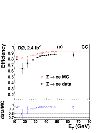
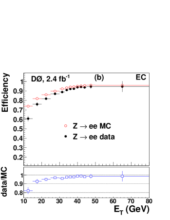
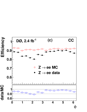
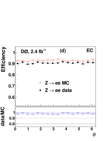
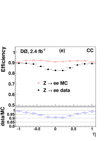
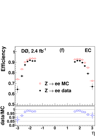
Figure 12: Electron identification efficiencies as a function of (a,b) $E_{T}$, (c,d) $\phi$ and (e,f) $\eta$ for loose electron requirements in CC and EC. Efficiencies for data and MC simulated $Z\to ee$ events are shown, as is the ratio of the data and MC efficiencies.

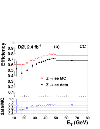
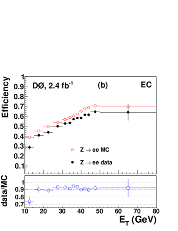
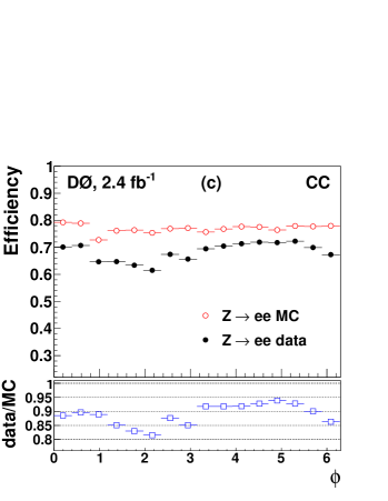
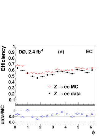
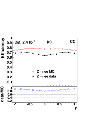
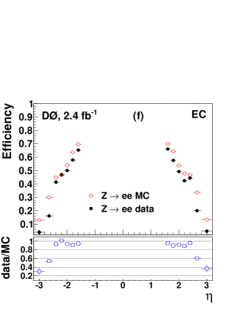
Figure 13: Electron identification efficiencies as a function of (a,b) $E_{T}$, (c,d) $\phi$ and (e,f) $\eta$ for tight electron requirements in CC and EC. Displayed are data and MC predictions in $Z\to ee$ decays and their ratio.

To account for deficiencies of the simulation, the simulation is corrected by applying $\eta$ and $\phi$ dependent correction factors. The dependence on instantaneous luminosity for the electron reconstruction efficiencies is studied and derived following ($\eta-\phi$)-dependent correction. Relative to the efficiency at low instantaneous luminosity ($\mathcal{L}_{\rm inst}$ $<$ $1.5\times 10^{32}$ cm^-2s^-1) the efficiency decreases with increasing $\mathcal{L}_{\rm inst}$, declining by $\approx$10% when $\mathcal{L}_{\rm inst}$ $=$ $2.5\times~{}10^{32}$ cm^-2s^-1. The ratio of those efficiencies in data and MC simulation has no dependence on the instantaneous luminosity.

For transverse momenta of $40$ GeV after preselection, loose electrons have a total identification efficiency of 85% (95%) with a fake rate from misidentified jets of 5% (3%) in the CC (EC). Tight electrons at the same transverse momentum have an identification efficiency of 72% (53%) with a misidentification rate of 0.2% (0.1%) in the CC (EC).

VIII Efficiencies of photon identification

VIII.1 Photon identification efficiencies

There are two categories of variables for photon identification. Variables based mainly on shower information are used to reject misidentified jets. Tracking-based variables are used to separate electrons from photons. There are two main mechanisms by which photons can appear as electrons. First, if the photon has converted into an electron-positron pair in the inner tracking system, creating a reconstructed track. The probability for conversion is $\approx$6%, and we do not reconstruct these converted photons explicitly. Second, if a track from particles of the underlying event is pointing to the EM cluster. In both cases, the matched track information for a photon will tend to be different from a real electron.

Because a large sample of pure photons is not available in data, $Z\to ee$ events are used to derive efficiencies for variables based mainly on the calorimeter information. For tracking-based variables, the efficiencies are measured from reconstructed radiated photons in $Z\to\gamma\ell\ell\ (\ell=e,\mu)$ events in data and MC. In both cases, differences between data and MC event samples are analyzed to correct the efficiency in simulation.

Due to different needs in various physics analyses, various sets of photon identification requirements are developed. We provide here photon identification efficiencies for two different sets of photon identification requirements.

The first set of photon identification requirements considered is used in the search for $H\to\gamma\gamma$ decays hgg-ref1 ; hgg-ref2 . The signal is dominated by high-$p_{T}$ CC photons, and the analysis maximizes the photon signal acceptance. Photon candidates in the CC are required to fulfill the preselection requirements as described in Sect. VII.3. In addition, it is required that

• $\Sigma p_{T}^{\rm trk}<2$ GeV;

• $\sigma_{\phi}^{2}<18$ cm²;

• Output of $\gamma$NN5 $>0.1$.

In addition the following requirements are placed on track-based variables:

• P($\chi^{2}_{\rm spatial}$) $=$ $-1$;

• $D_{\rm hor}<0.9$.

The measured identification efficiencies using the non track-based variables in this selection are presented in Fig. 14 (left column) as a function of $E_{T}$, $\eta$ and $\phi$. The differences between data and MC are at the percent level and are constant in the presented distributions. Therefore, a single correction factor is applied to MC photon simulation.

The second set of photon identification requirements presented here is used for measurements of electroweak cross sections, such as the measurement of the $W\gamma$ production cross section wg-ref . Here, the photons tend to have low $E_{T}$ and a high background rejection is required. The EC photons used are required to fulfill the preselection criteria of Sect. VII.3 and to satisfy the following requirements:

• $\Sigma p_{T}^{\rm trk}<1.5$ GeV

• $\sigma_{\phi}^{2}<(7.3\cdot\eta^{2}-35.9\cdot|\eta|+45.7)$ cm²

• Output of $\gamma$NN4$>0.05$

In addition, a track-based requirement P($\chi^{2}_{\rm spatial}$) $<$ 0.001 is applied.

Figure 14 (right column) shows the identification efficiencies using the non track-based variables in this selection for data and MC. The difference between data and simulation depends on $\eta$. To take this into account, the correction to MC simulation is parametrized as a function of $\eta$.

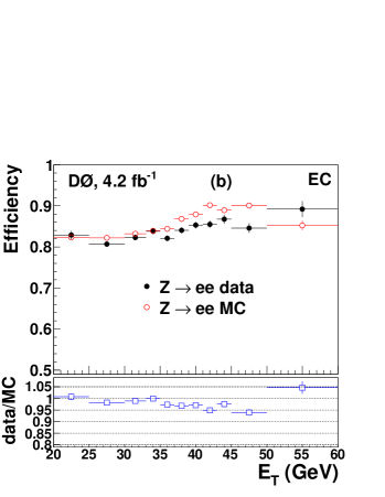
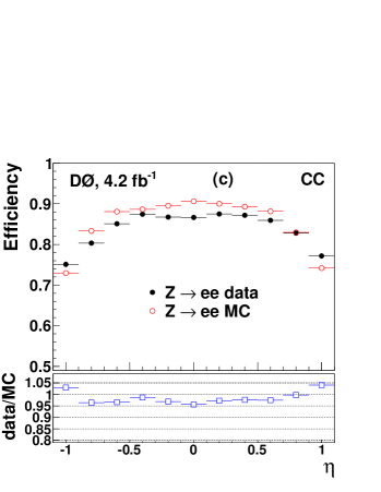
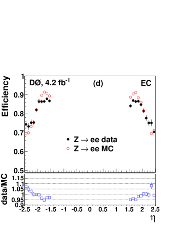
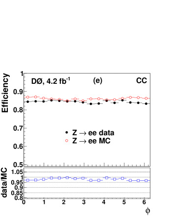
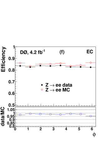
Figure 14: Photon identification efficiencies for identification variables mainly based on calorimeter information as derived from $Z\to ee$ decays. Displayed are data and MC predictions and their ratio as a function of $E_{T}$ (a) (b), $\eta$ (c) (d) and $\phi$ (e) (f) for CC and EC photons.

For both CC and EC photons, exploring the track-based variables as presented in this section, the efficiencies to identify a photon candidate are measured. The $Z\gamma\to\gamma\ell\ell$ $(\ell=e,\mu)$ data and MC comparison justifies that no further corrections to the photon simulation are required. The photon identification efficiency for these track-based variables is 92% (95%) in CC (EC) for an electron-to-photon misidentification rate of 2% (23%) in CC (EC) in the selections described above. The average photon identification efficiencies for the two sets of requirements described above are 81% and 83% for a rate to misidentify jets as photons of 4% and 10% for CC and EC photons, respectively. These identification efficiencies have a similar dependence on the instantaneous luminosity as the electron identification, and there is no visible dependence on the instantaneous luminosity for the ratio of those efficiencies in data and MC simulation.

VIII.2 Vertex pointing

In most physics applications, it is important to know from which $p\bar{p}$ collision vertex the photon originated. Since unconverted photons leave no track, the default reconstruction vertexing algorithm does not provide high probability to find the correct photon origin if there is no high-$p_{T}$ track in the event. For events without leptons and with energetic photons, the most probable photon production vertex can be reconstructed due to the presence of the underlying event coming from interactions of spectator quarks, and corresponds to the vertex with highest track multiplicity hgg-ref1 ; hgg-ref2 ; d0_dpp . In such cases, verifying that the true production vertex is found in data is important, especially in the high-instantaneous luminosity regime with many $p\bar{p}$ collision vertices.

To find the position of the photon origin along the beam line ($z$-axis) between $-$60 cm and 60 cm in the CC, the $(x,y,z)$-coordinates of the EM cluster in the EM1–EM4 layers and the position of the CPS cluster are used. Therefore, 5 points are used with radii from about 73 cm to 99 cm. Using a linear extrapolation to the $z$-axis, the most probable position of the photon origin vertex is obtained. Typical resolution of the algorithm varies between 3 and 4.5 cm. It becomes larger towards high $\eta$ mainly due to increasing amount of material in front of the calorimeter (from about $3.4$ to $5X_{0}$). The resolution has been tested in data using $Z(\to\ell\ell)+\gamma$ events, in which the “true” vertex ($z_{\rm true}$) is reconstructed using the two lepton ($e$ or $\mu$) tracks and the photon vertex ($z_{\rm point}$) is obtained using the procedure described above. The distribution of events for $\Delta z=z_{\rm true}-z_{\rm point}$ is shown in Fig. 15. The resolution is 2.4 cm for $|\eta|<0.4$, and 4.3 cm for $0.8<|\eta|<1.1$.

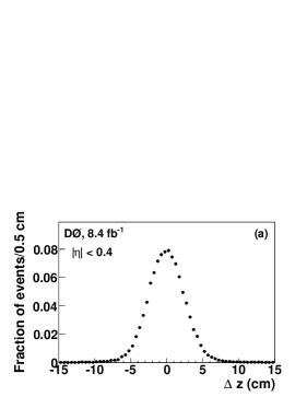
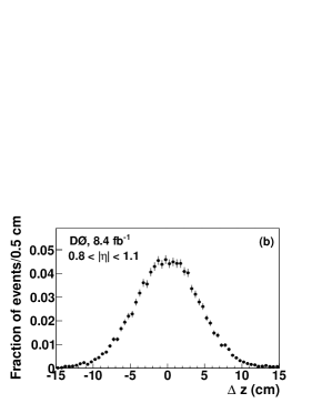
Figure 15: Vertex pointing resolution in two rapidity bins: $|\eta|<0.4$ (a), and $0.8<|\eta|<1.1$ (b).

The resolution in MC simulation is a factor of $1.4-1.5$ better than in data events. To calibrate the pointing resolution, a smearing procedure as a function of photon pseudorapidity is applied. The $\Delta z$ resolution is almost independent of photon $p_{T}$.

IX Conclusions

The precise and efficient reconstruction and identification of electrons and photons by the D0 experiment at the Tevatron $p\bar{p}$ collider at Fermilab is essential for a broad spectrum of physics analyses, including high precision SM measurements and searches for new phenomena.

In this paper, the electron and photon reconstruction and identification algorithms have been presented using data collected by the D0 detector in $p\bar{p}$ collisions at a center-of-mass energy of 1.96 TeV. The separation between electron or photon signal and multijet background is considerably improved using multivariate analysis techniques. A likelihood method for electron identification, a neural network method for electrons and photons, and a Boosted Decision Tree for electrons have been developed. An energy calibration dependent on the azimuthal angle of the EM cluster, the shower shape and the pseudorapidity has been performed separately for data and MC, leading to significant improvements in resolution and uniformity and resulting in a good agreement between data and MC.

Single electrons are triggered with an efficiency $\approx$100% for transverse momenta above 30 GeV in the fiducial regions of the calorimeter up to $|\eta|<2.5$. For transverse momenta of $E_{T}=40$ GeV, in general at D0 electrons can be identified with a total identification efficiency of 90% (95%) with the rate at which jets are misidentified as electrons being 5% (3%) in the CC (EC). Photons in the CC and EC regions can typically be identified with efficiencies varying between 69%–84% with the rate at which electrons or jets are misidentified as photons being 2%–10%.

The agreement of electron and photon identification efficiencies between data and MC in fiducial regions of the detector is reasonable, with deviations only at the percent level. Larger correction factors are necessary in non-fiducial regions close to the boundaries of the calorimeter modules. These correction factors have been applied to MC events as a function of kinematic variables resulting in considerable improvements of the simulation.

References

- (1) V. M. Abazov et al. (D0 Collaboration), Nucl. Instrum. Methods Phys. Res., Sect. A 565, 463 (2006).
- (2) V. M. Abazov et al. (D0 Collaboration), Phys. Rev. D 89, 012005 (2014).
- (3) V. M. Abazov et al. (D0 Collaboration), Phys. Rev. D 85, 052001 (2011).
- (4) V. M. Abazov et al. (D0 Collaboration), arXiv:1312.6873 [hep-ex].
- (5) V. M. Abazov et al. (D0 Collaboration), Nucl. Instrum. Methods Phys. Res., Sect. A 737, 281 (2014).
- (6) V. M. Abazov et al. (D0 Collaboration), Phys. Lett. B 698, 6 (2011).
- (7) M.L. Mangano et al., J. High Energy Phys. 07, 001 (2003). Version 2.11 is used.
- (8) T. Sjöstrand et al., J. High Energy Phys. 05, 026 (2006). Version 6.409 with Tune A is used.
- (9) V. M. Abazov et al. (D0 Collaboration), Phys. Rev. Lett. 100, 102002 (2008).
- (10) J. Pumplin et al., J. High Energy Phys. 07, 012 (2002); D. Stump et al., J. High Energy Phys. 10, 046 (2003).
- (11) R. Brun and F. Carminati, CERN Program Library Long Writeup W5013 (1993).
- (12) R. Engelmann et al, Nucl. Instrum. Meth. 216, 45 (1983).
- (13) S. Abachi et al. (D0 Collaboration), Nucl. Instrum. Meth. Phys. Res., Sect. A 324, 53 (1993).
- (14) L. Breiman et al., Classification and Regression Trees (Wadsworth, Stamford, 1984). Version v04-01-00 of TMVA is used.
- (15) C. Peterson, T. Rognvaldsson and L. Lonnblad, “JETNET 3.0 A versatile Artificial Neural Network Package”, Lund University Preprint LU-TP 93-29. Version 3.5 is used.
- (16) R. Wigmans, “Calorimetry”, Oxford University Press (2000).
- (17) R. Lopes, Ph.D. thesis, Stony Brook University, FERMILAB-THESIS-2013-13 (2013).
- (18) J. E. Gaiser, Ph.D. thesis, SLAC-R-236 (1980), Appendix D.
- (19) M. Vesterinen, Ph.D. thesis, University of Manchester, FERMILAB-THESIS-2011-35 (2011).
- (20) M. Abolins et al. (D0 Collaboration), Nucl. Instrum. Meth. Phys. Res., Sect. A 584, 75 (2008).
- (21) V. M. Abazov et al. (D0 Collaboration), Phys. Rev. Lett. 107, 151801 (2011).
- (22) V. M. Abazov et al. (D0 Collaboration), Phys. Rev. D 88, 052007 (2013).
- (23) V. M. Abazov et al. (D0 Collaboration), Phys. Rev. Lett. 107, 241803 (2011).
- (24) V. M. Abazov et al. (D0 Collaboration), Phys. Lett. B 690, 108 (2010).