Floer trajectories and stabilizing divisors

Abstract.

We incorporate pearly Floer trajectories into the transversality scheme for pseudoholomorphic maps introduced by Cieliebak-Mohnke [15]. By choosing generic domain-dependent almost complex structures we obtain zero and one-dimensional moduli spaces with the structure of cell complexes with rational fundamental classes. Integrating over these moduli spaces gives a definition of Floer cohomology over Novikov rings via stabilizing divisors for rational Lagrangians that are fixed point sets of anti-symplectic involutions satisfying certain Maslov index conditions as well as Hamiltonian Floer cohomology of compact rational symplectic manifolds. A subsequent paper [14] extends the techniques to regularization of moduli spaces needed for the definition of Fukaya algebras for more general Lagrangians.

1. Introduction

The Floer cohomology associated to a generic time-dependent Hamiltonian on a compact symplectic manifold is a version of Morse cohomology for the symplectic action functional on the space of paths between two Lagrangians [22], [23]. The cochains in this theory are formal combinations of Hamiltonian trajectories connecting the Lagrangians while the coboundary operator counts Hamiltonian-perturbed pseudoholomorphic strips. When well-defined, Floer cohomology is independent of the choice of Hamiltonian and can be used to estimate the number of intersection points as in the conjecture of Arnol^′d.

In order to construct the theory one must compactify the moduli spaces of Floer trajectories by allowing pseudoholomorphic disks and spheres, and unfortunately because of the multiple cover problem these moduli spaces can not be made regular in general using a fixed almost complex structure. In algebraic geometry there is now an elegant approach to this counting issue carried out in a sequence of papers by Behrend-Manin [10], Behrend-Fantechi [9], Kresch [37], and Behrend [8], based on suggestions of Li-Tian [38].

In symplectic geometry several methods for solving these transversality issues have been described. An approach using Kuranishi structures is developed in Fukaya-Ono [28] and a related approach in Liu-Tian [39]. Technical details have been further explained in Fukaya-Oh-Ohta-Ono [25] and McDuff-Wehrheim [43]. A polyfold approach has been developed by Hofer-Wysocki-Zehnder [34] and is being applied to Floer cohomology by Albers-Fish-Wehrheim [3]. See also Pardon [46] for an algebraic approach to constructing virtual fundamental chains. These approaches have in common that the desired perturbed moduli space should exist for abstract reasons.

On the other hand, it is very useful to have perturbations with geometric meaning whenever possible. For example, in the case of toric varieties, Fukaya et al [27] have pointed out that the general structure of the invariants is not enough to see that the Floer cohomology of Lagrangian torus orbits is well-defined, and one has to choose a perturbation system adapted to the geometric situation [27]. An approach to perturbing moduli spaces of pseudoholomorphic curves based on domain-dependent almost complex structures was introduced by Cieliebak-Mohnke [15] for symplectic manifolds with rational symplectic classes and further developed in Ionel-Parker [35] and Gerstenberger [31]. It was extended by Wendl [58] in genus zero to allow insertions of Deligne-Mumford classes. Domain-dependent almost complex structures can be made suitably generic only if one does not require invariance under automorphisms of the domain. Thus in order to obtain a perturbed moduli space, one must kill the automorphisms. This can be accomplished by choosing a stabilizing divisor: a codimension two almost complex submanifold meeting any pseudoholomorphic curve in a sufficient number of points. Approximately almost complex submanifolds of codimension two exist by a result of Donaldson [18]; the original almost complex structure can be perturbed so that the Donaldson submanifolds are exactly almost complex [15]. If the symplectic manifold admits a compatible complex structure which makes it a smooth projective variety, then Donaldson’s results are not necessary. Indeed, in this case the existence of suitable divisors follows from results of Bertini and Clemens [16].

We work under the following assumptions. Let $X$ be a compact connected symplectic manifold with symplectic form $\omega$ with $[\omega]\in H^{2}(X,\mathbb{Q})$ rational. A Lagrangian brane is a compact Lagrangian equipped with grading and relative spin structure, see Section 2.2 below. Results of Borthwick-Paul-Uribe [12, Theorem 3.12] in the Kähler case, and Auroux-Gayet-Mohsen [7] more generally, imply the existence of a stabilizing divisor in the complement of each Lagrangian such that each holomorphic disk meets the divisor at least once; the additional markings produced by the intersections allow us to achieve transversality using domain-dependent almost complex structures. To define Floer cohomology we will also need further conditions to rule out disk bubbling, which for lack of a better term we call admissibility; this definition is local to this paper.

Definition 1.1.

A Lagrangian $L\subset X$ is admissible if either

1. the Lagrangian

   $$L=\operatorname{\operatorname{graph}}(\psi)\subset X=Y^{-}\times Y$$

   is the graph of Hamiltonian diffeomorphism $\psi:Y\to Y$; here $Y^{-}$ denotes $Y$ with symplectic form reversed; or

2. the Lagrangian

   $$L=\{x\in X\ |\ \iota(x)=x\}\subset X$$

   is the fixed point set of an anti-symplectic involution

   $$\iota:X\to X,\quad\iota^{*}\omega=-\omega,$$

   has minimal Maslov number divisible by $4$, and is equipped with an $\iota$-relative spin structure in the sense of [26].

Floer cohomology of more general Lagrangians is constructed, following Fukaya-Oh-Ohta-Ono [24] who used Kuranishi structures, via stabilizing divisors in a follow-up paper [14] as a complex of bundles over the space of weak solutions to the Maurer-Cartan equation associated to the Fukaya algebra.

The main results of this paper are the following existence and invariance result for Floer cohomology groups. For $L_{0},L_{1}\subset X$ admissible Lagrangians, let $CF(L_{0},L_{1})$ denote the group of Floer cochains with rational Novikov coefficients. Denote by

$$\partial:CF(L_{0},L_{1})\to CF(L_{0},L_{1})$$

the coboundary operator defined by a rationally-weighted count of Floer trajectories in the zero-dimensional component of the moduli space.

Theorem 1.2.

Let $L_{0},L_{1}$ be admissible Lagrangian branes. There exists a comeager subset of a set of domain-dependent almost complex structures such that the moduli space of perturbed Floer trajectories of expected dimension at most one $\overline{\mathcal{M}}_{\leq 1}(L_{0},L_{1})$ has the structure of a cell complex with fundamental class in relative homology. The boundary of the locus of expected dimension one is the union of broken Floer trajectories consisting of pairs of Floer trajectories of expected dimension zero:

$$\partial[\overline{\mathcal{M}}_{1}(L_{0},L_{1})]=[{\mathcal{M}}_{0}(L_{0},L_{1})\times_{\mathcal{I}(L_{0},L_{1})}{\mathcal{M}}_{0}(L_{0},L_{1})].$$

The Floer coboundary operator $\partial$ is well-defined and satisfies $\partial^{2}=0$. The resulting Floer cohomology

$$HF(L_{0},L_{1})=\frac{\operatorname{ker}(\partial)}{\operatorname{im}(\partial)}$$

is independent of all choices and invariant under Hamiltonian perturbation of either Lagrangian. In the case $L_{0}=L_{1}=\Delta$ is equal to the diagonal Lagrangian $\Delta$ in a product $X=Y^{-}\times Y$, the Floer cohomology $HF(\Delta,\Delta)$ isomorphic to the singular cohomology of $Y$ with coefficients in the Novikov field.

Versions of this theorem, which includes a weak version of the Arnol^′d conjecture, appear in [26] and in Liu-Tian [39], and another version announced as [3]. However, abstract results such as the weak Arnol^′d conjecture are not the motivation for the approach presented here; rather we have various applications in mind in which the geometric meaning of the trajectories plays a role. Note that the proof of the weak Arnol^′d conjecture given here does not require the use of orbifolds (whose notion of morphism is very involved) nor virtual fundamental classes of any type, nor the transversality results for Floer trajectories in Floer-Hofer-Salamon [21].

We thank Mohammed Abouzaid, Eleny Ionel, Tom Parker, Nick Sheridan, Sushmita Venugopalan, and Chris Wendl for helpful discussions.

2. Floer trajectories

This section constructs a compactification of the moduli space of holomorphic strips with interior markings which allows the formation of bubbles on the boundary. The domains of these maps are nodal disks with two distinguished points. There are morphisms between moduli spaces of these disks of different combinatorial type, first studied by Knudsen [36] and Behrend-Manin [10]. These morphisms will play a key role in the construction of the perturbations.

2.1. Stable strips

We recall the definition of stable marked curves introduced by Mumford, Grothendieck and Knudsen [36]. By a nodal curve $C$ we mean a compact complex curve with only nodal singularities denoted $w_{1},\ldots,w_{l}\in C$ for some integer $l\geq 0$. A non-singular point of $C$ is a non-nodal point. For an integer $n\geq 0$, an $n$-marking of a nodal curve $C$ is a collection $\underline{z}\in C^{n}$ of distinct, non-singular points. A special point is a marking or node. An isomorphism of marked curves $(C_{0},\underline{z}_{0})$ to $(C_{1},\underline{z}_{1})$ is an isomorphism $C_{0}\to C_{1}$ mapping $\underline{z}_{0}$ to $\underline{z}_{1}$. Let $\operatorname{Aut}(C)=\operatorname{Aut}(C,\underline{z})$ be the group of automorphisms of $(C,\underline{z})$. A genus zero marked curve $(C,\underline{z})$ is stable if the group $\operatorname{Aut}(C)$ is trivial, or equivalently, any irreducible component of $C$ has at least three special points. The combinatorial type of a nodal marked curve $C$ is the graph $\Gamma$ whose vertices $\operatorname{Vert}(\Gamma)$ correspond to components of $C$ and edges $\operatorname{Edge}(\Gamma)$ consisting of finite edges $\operatorname{Edge}_{<\infty}(\Gamma)$ corresponding to nodes $w(e)\in C,e\in\operatorname{Edge}_{<\infty}(\Gamma)$ and semi-infinite edges $\operatorname{Edge}_{\infty}(\Gamma)$ corresponding to markings; the set of semi-infinite edges with a labelling $\operatorname{Edge}_{\infty}(\Gamma)\to\{1,\ldots,n\}$ so that the corresponding markings are $z_{1},\ldots,z_{n}\in C$. A connected curve $C$ has genus zero if and only if the graph $\Gamma$ is a tree and each irreducible component of $C$ has genus zero, that is, is isomorphic to the projective line. Knudsen [36] shows that the moduli space of stable genus zero $n$-marked connected curves has the structure of a smooth projective variety, and in particular, a smooth compact manifold. Let $\overline{\mathcal{C}}_{n}$ denote the moduli space of isomorphism classes of connected stable $n$-marked genus zero curves, with topology induced by Knudsen’s theorem [36]. For a combinatorial type $\Gamma$ let $\mathcal{C}_{\Gamma}$ the space of isomorphism classes of stable marked curves of type $\Gamma$. If $\Gamma$ is connected with $n$ semi-infinite edges we denote by $\overline{\mathcal{C}}_{\Gamma}$ the closure of $\mathcal{C}_{\Gamma}$ in $\overline{\mathcal{C}}_{n}$. We also allow disconnected curves $\Gamma$ whose components are genus zero, in which case we order the markings on each component and the combinatorial type $\Gamma$ is a forest (disjoint union of trees.) If $\Gamma=\sqcup_{i}\Gamma_{i}$ is disconnected then $\mathcal{C}_{\Gamma}=\prod_{i}\mathcal{C}_{\Gamma_{i}}$ is the product of the moduli spaces $\mathcal{C}_{\Gamma_{i}}$ for the component trees. Over $\overline{\mathcal{C}}_{n}$ there is a universal stable marked curve whose fiber over an isomorphism class of stable marked curve $[C,\underline{z}]$ is isomorphic to $C$.

The smooth structures on the moduli spaces can be described by deformation theory. Recall that a deformation of a nodal marked curve $(C,\underline{z})$ is a germ of a family $C_{B}\to B$ of nodal curves over a pointed scheme, say, $(B,b)$ together with sections $\underline{z}_{B}:B\to C_{B}^{n}$ corresponding to the markings and an isomorphism of the given marked curve $(C,\underline{z})$ with the fiber over $b\in B$. We omit the markings to simplify the notation. Any stable curve has a universal deformation $C_{B}\to B$, unique up to isomorphism, with the property that any other deformation is obtained via pullback by a unique map to $B$. The space of infinitesimal deformations $\operatorname{Def}(C)$ is the tangent space of $B$ at $b$. Similarly the tangential deformation space of a nodal marked curve $C$ of type $\Gamma$ is the space $\operatorname{Def}_{\Gamma}(C)$ of infinitesimal deformations of the complex structure fixing the combinatorial type. The deformation spaces sit in an exact sequence

$$0\to\operatorname{Def}_{\Gamma}(C)\to\operatorname{Def}(C)\to\mathcal{G}_{\Gamma}(C)\to 0$$

where

(1) $$\mathcal{G}_{\Gamma}(C)=\bigoplus_{e\in\operatorname{Edge}_{<\infty}(\Gamma)}T_{w(e)^{+}}^{\vee}C\otimes T_{w(e)^{-}}^{\vee}C$$

is the normal deformation space, see for example Arbarello-Cornalba-Griffiths [4, Chapter 11], and $T_{w(e)^{\pm}}C$ are the tangent spaces on either side of the corresponding nodes $w(e)\in C$. Elements of the normal deformation space are known as gluing parameters in symplectic geometry. Given a universal deformation of stable curves of fixed type $\Gamma$, the gluing construction produces a universal deformation by removing small disks around each node in a local coordinate $z$ and gluing the components together using maps $z\mapsto\delta_{e}/z$ where $\delta_{e}$ is the parameter corresponding to the $e$-th node. In genus zero there are several canonical schemes for choosing such local coordinates, for example, by using three special points on a component to fix an isomorphism with the projective line.

The moduli space of stable marked disks is a smooth manifold with corners as described in Fukaya-Oh-Ohta-Ono [24]. For integers $l,n\geq 0$, an $(l,n)$-marked disk is a stable $l+2n$-marked stable sphere $\hat{C}$ equipped with an anti-holomorphic involution $\iota_{\hat{C}}:\hat{C}\to\hat{C}$ such that the first $l$ markings are those on the fixed locus of the involution $\hat{C}^{*}$, and the quotient $C=\hat{C}/\iota_{\hat{C}}$ of the curve by the involution is a union of disk components (arising from components preserved by the involution and with non-empty fixed locus) and sphere components (arising from components interchanged by the involution). The markings fixed by the involution are boundary markings of $C$ while the remaining conjugated pairs of markings are interior markings of $C$. The deformation theory of stable disks is similar to that of stable spheres, except that the gluing parameters associated to the boundary markings will be assumed to be real non-negative:

(2) $$\mathcal{G}_{\Gamma}(C):=\bigoplus_{e\in\operatorname{Edge}_{d}(\Gamma)}(T_{w(e)^{+}}^{\vee}(\partial C)\otimes T_{w(e)^{-}}^{\vee}(\partial C))_{\geq 0}\\ \oplus\bigoplus_{e\in\operatorname{Edge}_{s}(\Gamma)}T_{w(e)^{+}}^{\vee}C\otimes T_{w(e)^{-}}^{\vee}C$$

where $\operatorname{Edge}_{d}(\Gamma)$ (resp. $\operatorname{Edge}_{s}(\Gamma)$) is the set of edges corresponding to boundary nodes connecting disk components (resp. interior nodes connecting sphere components to sphere or disk components), and $(T_{w(e)^{+}}^{\vee}(\partial C)\otimes T_{w(e)^{-}}^{\vee}(\partial C))_{\geq 0}\subset T_{w(e)^{+}}^{\vee}(\partial C)\otimes T_{w(e)^{-}}^{\vee}(\partial C)\cong\mathbb{R}$ is the non-negative part; the last isomorphism is induced from the natural orientations on the components of the boundary $\partial C$.

We introduce notation for moduli spaces of marked strips as follows. A marked strip is a marked disk with two boundary markings. Let $C$ be a connected $(2,n)$-marked nodal disk with markings $\underline{z}$. We write $\underline{z}=(z_{-},z_{+},z_{1},\ldots,z_{n})$ where $z_{\pm}$ are the boundary markings and $z_{1},\ldots,z_{n}$ are the interior markings. We call $z_{-}$ (resp. $z_{+}$) the incoming (resp. outgoing) marking. Let $C_{1},\ldots,C_{m}$ denote the ordered strip components of $C$ connecting $z_{-}$ to $z_{+}$; the remaining components are either disk components, if they have boundary, or sphere components, otherwise. Let $\tilde{w}_{i}:=C_{i}\cap C_{i+1}$ denote the intermediate node connecting $C_{i}$ to $C_{i+1}$ for $i=1,\ldots,m-1$. Let $\tilde{w}_{0}=z_{-}$ and $\tilde{w}_{m}=z_{+}$ denote the incoming and outgoing markings. Let $C^{\times}:=C-\{\tilde{w}_{0},\ldots,\tilde{w}_{m}\}$ denote the curve obtained by removing the nodes connecting strip components and the incoming and outgoing markings. Each strip component may be equipped with coordinates

$$\phi_{i}:C_{i}^{\times}:=C_{i}-\{\tilde{w}_{i},\tilde{w}_{i-1}\}\to\mathbb{R}\times[0,1],\quad i=1,\ldots,m$$

satisfying the conditions that if $j$ is the standard complex structure on $\mathbb{R}\times[0,1]$ and $j_{i}$ is the complex structure on $C_{i}$ then

$$\phi_{i}^{*}j=j_{i},\quad\lim_{z\to\tilde{w}_{i}}\pi_{1}\circ\phi_{i}(z)=-\infty,\quad\displaystyle\lim_{z\to\tilde{w}_{i+1}}\pi_{1}\circ\phi_{i}(z)=\infty$$

where $\pi_{i}$ denotes the projection on the $i^{th}$ factor. We denote by

(3) $$f:C^{\times}\to[0,1],\quad z\mapsto\pi_{2}\circ\phi_{i}(z)$$

the continuous map induced by the time coordinate on the strip components. The time coordinate is extended to nodal marked strips by requiring constancy on every connected component of $C^{\times}-\bigcup_{i}C^{\times}_{i}$. The boundary of any marked strip $C$ is partitioned as follows. For $b\in\{0,1\}$ denote

(4) $$(\partial C)_{b}:=f^{-1}(b)\cap\partial C$$

so that $\partial C^{\times}=(\partial C)_{0}\cup(\partial C)_{1}$. That is, $(\partial C)_{b}$ is the part of the boundary from $z_{-}$ to $z_{+}$, for $b=0$, and from $z_{+}$ to $z_{-}$ for $b=1$. An example of a stable strip is shown in Figure 1.

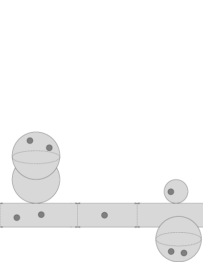
Figure 1. A stable marked strip

A variation on the definition of moduli spaces of stable disks or strips involves metric trees. A treed strip of type $\Gamma$ is a marked strip $(C,\underline{z})$ with a metric

$$\ell:\operatorname{Edge}_{<\infty,d}(\Gamma)\to[0,\infty]$$

assigning lengths to the finite edges of the subgraph of $\Gamma$ corresponding to disk components. The combinatorial type is defined as before, except that the subset of edges with infinite, zero or $]0,\infty[$ lengths is recorded as part of the data. Combinatorial types of strips naturally define combinatorial types of treed strips by adding zero metrics on their edges corresponding to boundary nodes. An isomorphism of treed marked strips is an isomorphism of marked strips having the same metric. A stable treed strip is one that has a stable underlying strip. Constructions of this type appear in, for example, Oh [45], Cornea-Lalonde [17], Biran-Cornea [11], and Seidel [54] and stable treed strips can be seen as special cases of the domain spaces used in [13]. There is a natural notion of convergence of treed stable strips, in which degeneration to a nodal disk assigns length zero to the node that appears. Let $\overline{\mathcal{M}}_{n}$ denote the moduli space of isomorphism classes of connected stable treed strips with $n$ interior markings in addition to the incoming and outgoing markings. For $\Gamma$ a connected type we denote by ${\mathcal{M}}_{\Gamma}\subset\overline{\mathcal{M}}_{n}$ the moduli space of stable strips of combinatorial type $\Gamma$ and $\overline{\mathcal{M}}_{\Gamma}$ its closure. Each $\overline{\mathcal{M}}_{\Gamma}$ is naturally a manifold with corners, with local charts obtained by a standard gluing construction. Generally $\overline{\mathcal{M}}_{n}$ is the union of several top-dimensional strata. In Figure 2 the locus in $\overline{\mathcal{M}}_{1}$ where the first marking has time coordinate $1/2$ is depicted (the stratum where the two interior markings come together to form a sphere bubble is not shown.)

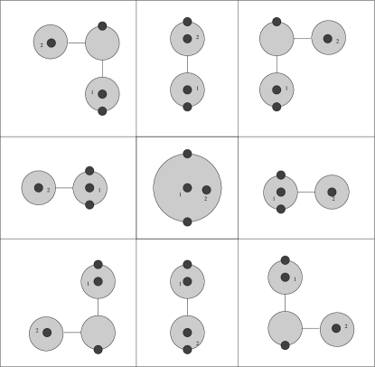
Figure 2. Stable treed disks

For $\Gamma$ disconnected, $\overline{\mathcal{M}}_{\Gamma}$ is the product $\prod_{i}\overline{\mathcal{M}}_{\Gamma_{i}}$ of moduli spaces for the connected components $\Gamma_{i}$ of $\Gamma$.

Orientations on the strata in the moduli space of treed disks may be constructed as follows (see Charest [13] for a more general procedure). Each stratum is a product of moduli spaces for the disk components and the intervals corresponding to the length parameters. For the case of a single disk, $m+2$ markings on the boundary and $n$ points in the interior, the moduli space may be identified with the subset of distinct tuples in

(5) $$\{(w_{1},\ldots,w_{m},z_{1},\ldots,z_{n})\in\mathbb{R}\backslash(\mathbb{R}\times\{0,1\})^{m}\times(\mathbb{R}\times(0,1))^{n}\}.$$

As a result, it inherits an orientation from the orientation on $\mathbb{R}\times[0,1]$ and the orientation on $\mathbb{R}$. In particular, note that the configuration with $m=1,n=0$ and the points $w_{1}$ lying in $\mathbb{R}\times\{0\}$ resp. $\mathbb{R}\times\{1\}$ has orientation given by $-1$ resp. $+1$ times the orientation of a point. If the disk has a single special point on the boundary then its interior may be identified with the positive half-space $\mathbb{H}\subset\mathbb{C}$. The moduli space $\mathcal{M}_{\Gamma}$ of disks with a single marking on the boundary and $n$ points in the interior is the subset of distinct tuples in

$$\mathcal{M}_{\Gamma}\cong\operatorname{Aut}(\mathbb{H})\backslash\{(z_{1},\ldots,z_{n})\in\mathbb{H}^{n}\}$$

where $\operatorname{Aut}(\mathbb{H})$ is the Lie group of automorphisms of the upper half-plane $\mathbb{H}$. Now $\operatorname{Aut}(\mathbb{H})$ is generated by translations and dilations, and this identifies $\operatorname{aut}(\mathbb{H})$ with $\mathbb{R}^{2}$ and so gives $\operatorname{Aut}(\mathbb{H})$ an orientation. The moduli space is oriented by the orientation on $\mathbb{H}^{n}$ and $\operatorname{Aut}(\mathbb{H})$. In general, any stratum $\mathcal{M}_{\Gamma}$ of $\overline{\mathcal{M}}_{n}$ is oriented by taking the product of the orientations for the disk components and strip components and the product of the intervals corresponding to lengths of the edges. The resulting orientation depends on the ordering of components and edges. However, the constructions below involve only the case of one disk component with only one boundary special point (in which case the moduli space has even dimension and the ordering is irrelevant) and at most two strip components (in which case the one containing the incoming marking is ordered first, and at most one interval corresponding to an edge with non-zero length). In particular, if $\Gamma$ is a type with a single disk bubble attached to $\mathbb{R}\times\{0\}$ resp. $\mathbb{R}\times\{1\}$ by an edge of zero length and $\Gamma^{\prime}$ is the type obtained by collapsing an edge then the map $\mathcal{M}_{\Gamma}\to\overline{\mathcal{M}}_{\Gamma^{\prime}}$ is orientation preserving resp. reversing.

Our perturbations will be maps defined on certain universal curves over the moduli spaces above. The moduli space of treed strips of each fixed type admits a universal strip

$$\overline{\mathcal{U}}_{\Gamma}\to\overline{\mathcal{M}}_{\Gamma}$$

whose fiber over an element $[C,\underline{z},\ell]\in\overline{\mathcal{M}}_{\Gamma}$ is the underlying stable marked disk $S=(C,\underline{z})$ without the metric. The universal strip is closely related to the moduli space $\overline{\mathcal{M}}_{\Gamma^{\prime}}$ of strips of the type $\Gamma^{\prime}$ obtained from $\Gamma$ by adding an additional interior marking; the two spaces are homeomorphic away from the boundary nodes (where the latter has real blowups). In particular, $\overline{\mathcal{U}}_{\Gamma}$ is a manifold with corners away from the boundary nodes. Later we will use local trivializations $\overline{\mathcal{U}}_{\Gamma}$ of the universal strip on each stratum $\mathcal{M}_{\Gamma}$ giving rise to families of complex structures. For a combinatorial type $\Gamma$ and a treed disk $C$ of type $\Gamma$ let

(6) $${{\mathcal{U}}}_{\Gamma}^{i}\to{{\mathcal{M}}}_{\Gamma}^{i}\times S,\quad i=1,\ldots,l$$

be a collection of local trivializations of the universal strip identifying each nearby fiber with $S$ in a way that the markings are constant. Let $\mathcal{J}(S)$ denote the space of complex structures on the smooth curve underlying $C$, or equivalently, the space of complex structures on its normalization of $C$ obtained by blowing up each node (so each node gets replaced with a pair of points). The complex structures on the fibers induce a map

(7) $${\mathcal{M}}_{\Gamma}^{i}\to\mathcal{J}(S),\ m\mapsto j(m).$$

Since the universal curve is locally holomorphically trivial in a neighborhood of the nodes and markings (see for example [4, Chapter 11] for the case of curves without boundary) we may assume that $j(m)$ is independent of $m$ on neighborhoods of the nodes and markings of $S$.

The combinatorial structure of the moduli spaces of stable treed strips involves identifications between moduli spaces of different combinatorial types introduced in Knudsen [36] and Behrend-Manin [10] in the case of stable curves. Families of perturbations will later be chosen to be coherent with respect to those identifications. In Behrend-Manin [10], these morphisms were associated to morphisms of graphs called extended isogenies. Here we call them Behrend-Manin morphisms.

Definition 2.1.

(Behrend-Manin morphisms of graphs) A morphism of graphs $\Upsilon:\Gamma\to\Gamma^{\prime}$ is a surjective map of the set of vertices $\operatorname{Vert}(\Gamma)\to\operatorname{Vert}(\Gamma^{\prime})$ obtained by combining the following elementary morphisms:

1. (Cutting edges) $\Upsilon$ cuts an edge $e\in\operatorname{Edge}_{<\infty,d}(\Gamma)$ with infinite length or an edge $e\in\operatorname{Edge}_{<\infty,s}(\Gamma)$ if $\Upsilon$ is a bijection but the edge sets are related by

   $$\operatorname{Edge}(\Gamma^{\prime})\cong\operatorname{Edge}(\Gamma)-\{e\}+\{e_{+},e_{-}\}$$

   where $e_{\pm}$ are semi-infinite edges attached to the vertices contained in $e$. Since our curves have genus zero, $\Gamma^{\prime}$ is disconnected with pieces $\Gamma_{-},\Gamma_{+}$. If the edge corresponds to a node connecting disk components then $\Gamma_{-},\Gamma_{+}$ are types of stable disks, while if the edge corresponds to a node connecting a disk or sphere to a sphere component then one type, say $\Gamma_{-}$ is the type of a stable disk while $\Gamma_{+}$ is the type of a stable sphere. The ordering on $\operatorname{Edge}_{\infty,s}(\Gamma)$ induces one on $\operatorname{Edge}_{\infty,s}(\Gamma_{\pm})$ by using on $e_{\pm}$ the lowest value label on $\operatorname{Edge}_{\infty,s}(\Gamma_{\mp})$.

2. (Collapsing edges) $\Upsilon$ collapses an edge if the map on vertices $\Upsilon:\operatorname{Vert}(\Gamma)\to\operatorname{Vert}(\Gamma^{\prime})$ is a bijection except for a single vertex $v^{\prime}\in\operatorname{Vert}(\Gamma^{\prime})$ which has two pre-images connected by an edge in $\operatorname{Edge}(\Gamma)$ of length zero, and

   $$\operatorname{Edge}(\Gamma^{\prime})\cong\operatorname{Edge}(\Gamma)-\{e\}.$$

3. (Making an edge finite or non-zero) $\Upsilon$ makes an edge finite or non-zero if $\Gamma$ is the same graph as $\Gamma^{\prime}$ and the lengths of the edges $\ell(e),e\in\operatorname{Edge}(\Gamma^{\prime})$ are the same except for a single edge for which $\ell(e)=\infty$ resp. $0$ and the length $\ell^{\prime}(e)$ in $\Gamma^{\prime}$ is in $(0,\infty)$.

4. (Forgetting tails) $\Upsilon:\Gamma\to\Gamma^{\prime}$ forgets a tail (semi-infinite edge) and collapses edges that become unstable. The ordering on $\operatorname{Edge}_{\infty,s}(\Gamma)$ then naturally defines one on $\operatorname{Edge}_{\infty,s}(\Gamma^{\prime})$.

Each of the above operations on graphs corresponds to a map of moduli spaces of stable marked disks.

Definition 2.2.

(Behrend-Manin maps of moduli spaces)

1. (Cutting edges) Suppose that $\Gamma^{\prime}$ is obtained from $\Gamma$ by cutting an edge. A diffeomorphism $\overline{\mathcal{M}}_{\Gamma^{\prime}}\to\overline{\mathcal{M}}_{\Gamma}$ obtained by identifying the two markings corresponding to the cut edge and choosing the ordering of the markings to correspond to the non-identified markings of the original curve.

2. (Collapsing edges) Suppose that $\Gamma^{\prime}$ is obtained from $\Gamma$ by collapsing an edge. There is an embedding $\overline{\mathcal{M}}_{\Gamma}\to\overline{\mathcal{M}}_{\Gamma^{\prime}}$ with normal bundle having fiber at $[C]$ isomorphic to the space $\mathcal{G}_{\Gamma^{\prime}}(C)/\mathcal{G}_{\Gamma}(C)$, see (2). The image of such an embedding is a 1-codimensional corner of $\overline{\mathcal{M}}_{\Gamma^{\prime}}$.

3. (Making an edge finite resp. non-zero ) If $\Gamma^{\prime}$ is obtained from $\Gamma$ by making an edge finite resp. non-zero then $\overline{\mathcal{M}}_{\Gamma}$ also embeds in $\overline{\mathcal{M}}_{\Gamma^{\prime}}$ as the 1-codimensional corner where $e$ reaches infinite resp. zero length, with trivial normal bundle.

4. (Forgetting tails) Suppose that $\Gamma^{\prime}$ is obtained from $\Gamma$ by forgetting the $i$-th tail. Forgetting the $i$-th marking and collapsing the unstable components and sum distances for the glued edges defines a map $\overline{\mathcal{M}}_{\Gamma}\to\overline{\mathcal{M}}_{\Gamma^{\prime}}$.

Most of these maps were already considered by Knudsen [36] and might also be called Knudsen maps. Each of the maps involved in the operations (Collapsing edges), (Making edges finite or non-zero), (Forgetting tails), (Cutting edges) extends to a smooth map of universal treed strips. In the case that $\Gamma$ is disconnected, say the disjoint union of $\Gamma_{1}$ and $\Gamma_{2}$, then $\overline{\mathcal{M}}_{\Gamma}\cong\overline{\mathcal{M}}_{\Gamma_{1}}\times\overline{\mathcal{M}}_{\Gamma_{2}}$. In this case the universal treed strip $\overline{\mathcal{U}}_{\Gamma}$ is the disjoint union of the pullbacks of the universal treed strip $\overline{\mathcal{U}}_{\Gamma_{1}}$ and $\overline{\mathcal{U}}_{\Gamma_{2}}$.

We recall the definition of the morphisms in (Forgetting a tail). Let $(C,z_{1},\ldots,z_{n},\ell)$ be a stable treed marked strip with $n$ interior markings $z_{1},\ldots,z_{n}$. Given an integer $i\in\{1,\ldots,n\}$, we obtain an $n-1$-marked treed strip $(C,z_{1},\ldots,\hat{z_{i}},z_{n},\ell)$ by forgetting the $i$-th marking. The unstable components can be collapsed as follows:

1. If a sphere component $C_{k}\subset C$ becomes unstable after forgetting the $i$-th marking, having only two remaining special points $w^{\prime},w^{\prime\prime}\in C_{k}$, collapse the component, identifying the remaining special points $w^{\prime}\sim w^{\prime\prime}$;

2. If a disk or strip component $C_{k}\subset C$ becomes unstable after forgetting the $i$-th marking, starting from the component containing the $i$-th marking, iteratively collapse the unstable disk components $C_{i_{1}},\ldots,C_{i_{l}}$, identifying the boundary special points if there are more than one or forgetting it whenever there is only one. At every step, if the collapsed disk $C_{i_{l}}$ has only one node $w\in C_{i_{l}}$ with a metric, that metric should be forgotten (the node itself is forgotten), while if it has two nodes $w^{\prime},w^{\prime\prime}$ with a metric, those metrics should be summed and the two node identified to obtain a node $w\sim w^{\prime}\sim w^{\prime\prime}$ with length $\ell(w)=\ell(w^{\prime})+\ell(w^{\prime\prime})$.

The universal strip is equipped with the following maps. On the universal strip, the time coordinates (3) on the strip components extend to a map

(8) $$f:\overline{\mathcal{U}}_{\Gamma}\to[0,1]$$

On the subset with time coordinate equal to zero or one, we have additional maps measuring the distance to the strip components given by summing the lengths of the connecting edges:

$$\ell_{b}:f^{-1}(b)\to[0,\infty],\quad z\mapsto\sum_{e\in\operatorname{Edge}(z)}\ell(e),\quad b\in\{0,1\}$$

where $\operatorname{Edge}(z)$ is the set of edges corresponding to nodes between $z$ and the strip components. Thus any point on the universal strip $z\in\overline{\mathcal{U}}_{\Gamma}$ which lies on a disk component has $f(z)\in\{0,1\}$ and so $\ell_{b}(z)$ is well-defined for either $b=0$ or $b=1$.

2.2. Floer trajectories

We now turn to Floer theory. First we describe the space of Floer cochains. Recall that $(X,\omega)$ is a compact symplectic manifold. Let Lagrangians $L_{0},L_{1}\subset X$ be admissible Lagrangian branes. Let $H\in C^{\infty}([0,1]\times X)$ be a time-dependent Hamiltonian and let

$$\widehat{H}\in\operatorname{Map}([0,1],\operatorname{Vect}(X)),\quad\iota(\hat{H})\omega={\operatorname{d}}H$$

denote its Hamiltonian vector field with time $t$ flow $\phi_{t}:X\to X$. Denote by

$$\mathcal{I}(L_{0},L_{1}):=\left\{x:[0,1]\to X\ |\ \frac{d}{dt}x=\widehat{H}\circ x,\quad x(b)\in L_{b},b\in\{0,1\}\right\}\cong\phi_{1}(L_{0})\cap L_{1}$$

the set of perturbed intersection points, assumed to be transverse.

We are particularly interested in the special case of the diagonal. That is, suppose that $Y$ is a compact symplectic manifold, $Y^{-}$ is the symplectic manifold obtained by reversing the symplectic form and $X=Y^{-}\times Y$. Let

$$\Delta=\{(y,y)\ |\ y\in Y\}\subset X$$

denote the diagonal Lagrangian. In the case that $L_{0}=L_{1}=\Delta$ there is a bijection between perturbed intersection points and the space of one-periodic orbits,

$$\mathcal{I}(L_{0},L_{1})=\left\{x:S^{1}\to X\ |\ \frac{d}{dt}x=\widehat{H}\circ x\right\}\cong\{x\in X\ |\ \phi_{1}(x)=x\}.$$

A degree map on the set of intersection points is induced from gradings on the Lagrangians. Suppose that $X$ is equipped with an $N$-fold Maslov cover $\operatorname{Lag}^{N}(X)\to\operatorname{Lag}(X)$ for some positive integer $N$; recall from Seidel [53, Lemma 2.6] that $(X,\omega)$ admits an $N$-fold Maslov covering if and only if $N$ divides twice the minimal Chern number. A grading of a Lagrangian $L$ is a lift of the canonical section $L\to\operatorname{Lag}(X)$ to $\operatorname{Lag}^{N}(X)$. Given gradings on $L_{0},L_{1}$, the intersection set $\mathcal{I}(L_{0},L_{1})$ is equipped with a degree map

$$\mathcal{I}(L_{0},L_{1})\to\mathbb{Z}_{N},\quad x\mapsto|x|.$$

Denote by $\mathcal{I}(L_{0},L_{1})_{k}=\{x\in\mathcal{I}(L_{0},L_{1})\ |\ |x|=k\}$ the subset of degree $k$ so that

$$\mathcal{I}(L_{0},L_{1})=\bigcup_{k\in\mathbb{Z}_{N}}\mathcal{I}(L_{0},L_{1})_{k}.$$

The Floer cochains form a cyclically-graded group generated by the time-one periodic trajectories. Let $\Lambda$ be the universal Novikov field in a formal parameter $q$,

$$\Lambda=\left\{\sum_{\rho\in\mathbb{R}}a(\rho)q^{\rho},\quad\forall\epsilon,\operatorname{supp}(a)\cap(-\infty,\epsilon)<\infty,\quad a(\mathbb{R})\subset\mathbb{Q}\right\}.$$

Products in $\Lambda$ are defined by $q^{\rho_{1}}q^{\rho_{2}}=q^{\rho_{1}+\rho_{2}}$ for $\rho_{1},\rho_{2}\in\mathbb{R}$, and extended to linear combinations. Let $CF(L_{0},L_{1})$ denote the free $\Lambda$-module generated by $\mathcal{I}(L_{0},L_{1})$,

$$CF(L_{0},L_{1})=\bigoplus_{k\in\mathbb{Z}_{N}}CF^{k}(L_{0},L_{1}),\quad CF^{k}(L_{0},L_{1})=\bigoplus_{x\in\mathcal{I}(L_{0},L_{1})_{k}}\Lambda<\kern-3.01385pt{x}\kern-3.01385pt>.$$

The coboundary operator in Floer cohomology is defined by counting Floer trajectories. To describe Floer’s equation we introduce notations for almost complex structures and associated decompositions. We have the following notation for almost complex structures on surfaces. Let $C$ be an oriented surface, possibly with non-empty boundary $\partial C$. Denote by $\mathcal{J}(C)$ the space of complex structures $j:C\to C$ compatible with the orientation. Let $E\to C$ be a complex vector bundle and let $\Omega^{1}(C,E)$ denote the space of one-forms with values in $E$, that is, sections of $T^{\vee}C\otimes_{\mathbb{R}}E$. Given $\alpha\in\Omega^{1}(C,E)$ and a complex structure $j\in\mathcal{J}(C)$, denote by $\alpha^{0,1}\in\Omega^{0,1}(C,E)$ its $0,1$-part with respect to the decomposition

$$T^{\vee}C\otimes_{\mathbb{R}}E=(T^{\vee}C\otimes_{\mathbb{R}}E)^{1,0}\oplus(T^{\vee}C\otimes_{\mathbb{R}}E)^{0,1}.$$

We introduce the following terminology for almost complex structures. An almost complex structure $J:TX\to TX$ is $\omega$-tamed if $\omega(\cdot,J\cdot)$ is positive, and $\omega$-compatible if $\omega(\cdot,J\cdot)$ is a Riemannian metric. Denote by $\mathcal{J}_{\tau}(X,\omega)$ the space of $\omega$-tamed almost complex structures and by $\mathcal{J}(X,\omega)$ the space of $\omega$-compatible almost complex structures. In the following paragraphs, let $J\in\mathcal{J}_{\tau}(X,\omega)$.

Next we introduce notations for Hamiltonian perturbations and associated perturbed Cauchy-Riemann operators. Let $K\in\Omega^{1}(C,\partial C;C^{\infty}(X))$ be a one-form with values in smooth functions vanishing on the tangent space to the boundary, that is, a smooth map $TC\times X\to\mathbb{R}$ linear on each fiber of $TC$, equal to zero on $TC|\partial C$. Denote by $\widehat{K}\in\Omega^{1}(C,\partial C;\operatorname{Vect}(X))$ the corresponding one form with values in Hamiltonian vector fields. The curvature of the perturbation is

(9) $$R_{K}={\operatorname{d}}K+\{K,K\}/2\in\Omega^{2}(C,C^{\infty}(X))$$

where $\{K,K\}\in\Omega^{2}(C,C^{\infty}(X))$ is the two-form obtained by combining wedge product and Poisson bracket, see McDuff-Salamon [44, Lemma 8.1.6] whose sign convention is slightly different. Given a map $u:C\to X$, define

(10) $$\overline{\partial}_{J,K}u:=({\operatorname{d}}u+\widehat{K})^{0,1}\in\Omega^{0,1}(C,u^{*}TX).$$

The map $u$ is (J,K)-holomorphic if $\overline{\partial}_{J,K}u=0$. Suppose that $C$ is equipped with a compatible metric and $X$ is equipped with a tamed almost complex structure and perturbation $K$. The $K$-energy of a map $u:C\to X$ is

$$E_{K}(u):=(1/2)\int_{C}|{\operatorname{d}}u+\widehat{K}(u)|_{J}^{2}$$

where the integral is taken with respect to the measure determined by the metric on $C$ and the integrand is defined as in [44, Lemma 2.2.1]. If $\overline{\partial}_{J,K}u=0$, then the $K$-energy differs from the symplectic area $A(u):=\int_{C}u^{*}\omega$ by a term involving the curvature from (9):

(11) $$E_{K}(u)=A(u)+\int_{C}R_{K}(u).$$

In particular, if the curvature vanishes then the area is non-negative.

The notion of Floer trajectory is obtained from the notion of perturbed pseudoholomorphic map by specializing to the case of a strip

$$C=\mathbb{R}\times[0,1]=\{(s,t)\ |\ s\in\mathbb{R},t\in[0,1]\}.$$

Given $H\in C^{\infty}([0,1]\times X)$ let $K$ denote the perturbation one-form $K=-H{\operatorname{d}}t$ and let $E_{H}:=E_{K}$. If $u:\mathbb{R}\times[0,1]\to X$ has limits $x_{\pm}:[0,1]\to X$ as $s\to\pm\infty$ then the energy-area relation (11) becomes

$$E_{H}(u)=A(u)-\int_{[0,1]}(x_{+}^{*}H-x_{-}^{*}H){\operatorname{d}}t.$$

Let $\overline{\partial}_{J,H}=\overline{\partial}_{J,K}$ be the corresponding perturbed Cauchy-Riemann operator from (10). A map $u:C\to X$ is $(J,H)$-holomorphic if $\overline{\partial}_{J,H}u=0$. A Floer trajectory for Lagrangians $L_{0},L_{1}$ is a finite energy $(J,H)$-holomorphic map $u:\mathbb{R}\times[0,1]\to X$ with $\mathbb{R}\times\{b\}\subset L_{b},b=0,1$. An isomorphism of Floer trajectories $u_{0},u_{1}:\mathbb{R}\times[0,1]\to X$ is a translation $\psi:\mathbb{R}\times[0,1]\to\mathbb{R}\times[0,1]$ in the $\mathbb{R}$-direction such that $\psi^{*}u_{1}=u_{0}$. Denote by

$$\mathcal{M}(L_{0},L_{1}):=\left\{u:\mathbb{R}\times[0,1]\to X\ |\begin{array}[]{c}\overline{\partial}_{J,H}u=0\\ u(\mathbb{R}\times\{b\})\subset L_{b},b\in\{0,1\}\\ E_{H}(u)<\infty\end{array}\right\}/\mathbb{R}$$

the moduli space of isomorphism classes of Floer trajectories of finite energy, with its quotient topology.

In order to apply the theory of Donaldson hypersurfaces we will need our Hamiltonian perturbations to vanish, and in order to achieve recall the correspondence between Floer trajectories with Hamiltonian perturbation and trajectories without perturbation with different boundary condition. Let $H\in C^{\infty}([0,1]\times\mathbb{R},X)$ be a time-dependent Hamiltonian and let $J\in\operatorname{Map}([0,1],\mathcal{J}_{\tau}(X,\omega))$ be a time-dependent almost complex structure. Suppose that $L_{0},L_{1}$ are Lagrangians such that $\phi_{1}(L_{0})\cap L_{1}$ is transversal. There is a bijection between $(J_{t},H_{t})$-holomorphic Floer trajectories with boundary conditions $L_{0},L_{1}$ and $(\phi_{1-t}^{-1})^{*}J_{t}$-holomorphic Floer trajectories with boundary conditions $\phi_{1}(L_{0}),L_{1}$ obtained by mapping each $(L_{0},L_{1})$ trajectory $(s,t)\mapsto u(s,t)$ to the $(\phi_{1}(L_{0}),L_{1})$-trajectory given by $(s,t)\mapsto\phi_{1-t}(u(s,t))$ [21, Discussion after (7)].

A compactification of the space of Floer trajectories is obtained by allowing sphere and disk bubbling. A nodal Floer trajectory consists of a nodal strip $C$ together with a map $u:C\to X$ satisfying the following conditions:

1. $u((\partial C)_{b})\subset L_{b}$ for $b\in\{0,1\}$ (see (4))

2. $u$ is $(J_{t},H_{t})$-holomorphic in strip coordinates on each strip component $C_{i}-\{w_{i},w_{i+1}\}$ and

3. $u$ is $J_{t}$-holomorphic on each sphere and disk component on which $f$ is constant and equal to $t$; see (4) for the definition of $(\partial C)_{b}$.

An isomorphism of marked nodal Floer trajectories is an isomorphism of marked nodal curves with disk structures intertwining the markings and the maps to $X$. A marked nodal Floer trajectory $u:C\to X$ is stable if it has finitely many automorphisms, that is, $\#\operatorname{Aut}(u)<\infty$. A component $C_{v},v\in\operatorname{Vert}(\Gamma)$ of $C$ is a ghost component if the restriction of $u$ to $C_{v}$ has zero energy, that is, $E_{H}(u|C_{v})=0$. A nodal marked Floer trajectory $u:C\to X$ is stable if and only if any sphere ghost component $C_{v}\subset C$ has at least three special points $z_{i}\in C_{v},w_{k}\in C_{v}$ and any disk ghost component has either (a) at least three boundary special points or (b) one interior special point and one boundary special point. Let

$$\overline{\mathcal{M}}(L_{0},L_{1})=\left\{u:C\to X\ |\ \begin{array}[]{c}\overline{\partial}_{J,H}u=0,\ E_{H}(u)<\infty\\ \ u((\partial C)_{b})\subset L_{b},b\in\{0,1\}\end{array}\right\}/\sim$$

denote the moduli space of isomorphism classes of stable Floer trajectories of finite energy. $\overline{\mathcal{M}}(L_{0},L_{1})$ may be equipped with a topology similar to that of pseudoholomorphic maps, see for example McDuff-Salamon [44, Section 5.6]: Gromov-Floer convergence defines a topology in which convergence is Gromov-Floer convergence, by proving the existence of suitable local distance functions. Given $x_{\pm}\in\mathcal{I}(L_{0},L_{1})$, denote by

$$\overline{\mathcal{M}}(L_{0},L_{1},x_{+},x_{-}):=\left\{[u]\in\overline{\mathcal{M}}(L_{0},L_{1})\ |\ \lim_{s\to\pm\infty}u(s,\cdot)=x_{\pm}\right\}$$

the moduli space with fixed limits along the strip-like ends near $z_{\pm}\in\partial C$.

In preparation for the transversality arguments later, we review the Fredholm theory for the moduli space of Floer trajectories. Let $C$ be a treed strip of type $\Gamma$. We denote by $C^{\times}$ the curve with strip-like ends obtained by removing the nodes connecting strip components and incoming and outgoing markings. For integers $p>2$ and $k$ sufficiently large (for the moment, $k>2/p$ suffices) we denote by $\operatorname{Map}^{k,p}(C^{\times},X,\underline{L})$ the space of continuous maps of Sobolev class $W^{k,p}$ on each component $C_{v}\subset C^{\times}$ and taking the given Lagrangian boundary conditions:

$$\operatorname{Map}^{k,p}(C^{\times},X):=\left\{u:C^{\times}\to X,\ \forall m,\ \|u|C_{v}\|_{k,p}<\infty,\ u((\partial C_{b})\subset L_{b},b\in\{0,1\}\right\}.$$

Here the Sobolev $k,p$-norm $\|\cdot\|_{k,p}$ is defined using a covariant derivative on $X$ and $C^{\times}$ of standard form on the strip-like ends as in, for example, Schwarz [51]. Denote by $\Omega^{0}(C^{\times},u^{*}(TX,TL))_{k,p}$ the space of continuous sections of Sobolev class $k,p$ on each component, taking values in the pull-back $u^{*}TX$ of the cotangent bundle, and with boundary values in $(u|\partial C^{\times}_{b})^{*}TL_{b}$ on $\partial C^{\times}_{b}\subset\partial C$ on $f^{-1}(b)\cap\partial C$. Given time-dependent metrics that so that $L_{b}$ are totally geodesic for time $b\in\{0,1\}$, we have geodesic exponentiation maps

(12) $$\Omega^{0}(C^{\times},u^{*}(TX,T\underline{L}))_{k,p}\to\mathcal{B}_{k,p}:=\operatorname{Map}^{k,p}(C^{\times},X,\underline{L}),\quad\xi\mapsto\exp_{u}(\xi)$$

which provide charts for $\mathcal{B}_{k,p}$. With these charts $\mathcal{B}_{k,p}$ admits the structure of a smooth Banach manifold by standard Sobolev estimates. Define a fiber bundle $\mathcal{E}_{k,p}$ over $\mathcal{B}_{k,p}$ whose fiber at $u$ is

(13) $$(\mathcal{E}_{k,p})_{u}:=\Omega^{0,1}(C^{\times},u^{*}TX)_{k-1,p},$$

that is, a product of $(0,1)$-forms over the smooth components of $C^{\times}$. Local trivializations of $\mathcal{E}_{k,p}$ are defined by geodesic exponentiation from $u$ and parallel transport using the Hermitian connection defined by the almost complex structure

$$\Phi_{\xi}:\Omega^{0,1}(C^{\times},u^{*}TX)_{k-1,p}\to\Omega^{0,1}(C^{\times},\exp_{u}(\xi)^{*}TX)_{k-1,p}$$

see for example [44, p. 48]. The Cauchy-Riemann operator defines a section

(14) $$\overline{\partial}_{J,H}:\ \mathcal{B}_{k,p}\to\mathcal{E}_{k,p},\quad u\mapsto\overline{\partial}_{J,H}u.$$

Define a non-linear map on Banach spaces using the local trivializations

$$\mathcal{F}_{u}:\Omega^{0}(C^{\times},u^{*}(TX,T\underline{L}))_{k,p}\to\Omega^{0,1}(C^{\times},u^{*}(TX,T\underline{L}))_{k-1,p},\quad\xi\mapsto\Phi_{\xi}^{-1}\overline{\partial}_{J,H}\exp_{u}(\xi).$$

The quotient of the zero level set $\mathcal{F}_{u}^{-1}(0)/\operatorname{Aut}(C^{\times})$ is naturally identified with a subset of $\mathcal{M}(L_{0},L_{1})$ and gives a local description of the moduli space.

The local smoothness of the moduli space can be guaranteed by the surjectivity of the linearized operator by the implicit function theorem for maps between Banach spaces. Let $D_{u}$ denote the linearization of $\mathcal{F}_{u}$ (see Floer-Hofer-Salamon [21, Section 5]). Standard arguments show that this operator is Fredholm, see Lockhart-McOwen [40] and Donaldson [19, Section 3.4]. A stable non-nodal Floer trajectory $u:C^{\times}\to X$ is regular if $D_{u}$ is surjective. If $C=\mathbb{R}\times[0,1]$ and $u:C^{\times}\to X$ is a regular Floer trajectory then $\overline{\partial}_{J,H}^{-1}(0)$ is a smooth, finite dimensional manifold near $u$. The action of $\operatorname{Aut}(C)$ is free and proper, and the quotient is Hausdorff by exponential decay at the ends, equivalent to finiteness of the energy. It follows that $\mathcal{M}(L_{0},L_{1})$ is a smooth manifold near any regular $[u]$. Floer-Hofer-Salamon [21, Proof of Theorem 5.1] show, at least in the case of periodic Floer cohomology, that there exist time-dependent almost complex structures such that every Floer trajectory is regular. We avoid the use of [21] by using stabilizing divisors to construct coherent perturbations in the next section.

3. Coherent perturbations

In this section we describe how to regularize the moduli space of Floer trajectories using stabilizing divisors. We assume the reader is at least modestly familiar with the results of Cieliebak-Mohnke [15], which show how to use stabilizing divisors to kill the automorphisms of spheres appearing in the compactification of moduli spaces of pseudoholomorphic maps.

3.1. Stabilizing divisors

As mentioned in the introduction, our goal is to kill automorphism groups of disks appearing in the compactification by adding markings corresponding to intersection points with a codimension two symplectic submanifold produced by Donaldson’s construction. Because any such disk has at least one special point on the boundary, it suffices to choose divisors so that any non-constant holomorphic disk intersects the divisor at least once.

We introduce the following terminology. By a divisor we mean a closed codimension two symplectic submanifold $D\subset X$. An almost complex structure $J:TX\to TX$ is adapted to a divisor $D$ if $D$ is an almost complex submanifold of $(X,J)$.

Definition 3.1.

A divisor $D\subset X$ is stabilizing for a Lagrangian submanifold $L\subset X$ if and only if

1. the divisor $D$ is disjoint from the Lagrangian $L$, that is, $L\cap D=\emptyset$; and

2. any positive area disk $u:(C,\partial C)\rightarrow(X,L)$ intersects the divisor $D$ in at least one point: $\omega([u])>0\implies u^{-1}(D)\neq\emptyset.$

Example 3.2.

Suppose that the Lagrangian $L$ is exact in $(X-D,\omega)$, that is, for some one-form $\alpha\in\Omega^{1}(X-D)$ and function $\phi\in\Omega^{0}(L)$ we have ${\operatorname{d}}\alpha=\omega$ and ${\operatorname{d}}\phi=\alpha|_{L}$. In this case $D$ satisfies condition (b). Indeed, since $\omega=d\alpha$ on $X-D$ and $\alpha|L={\operatorname{d}}\phi$ for some $\phi:L\to\mathbb{R}$, the integral of $\omega$ over any disk $u:(C,\partial C)\rightarrow(X-D,L)$ vanishes:

$$\int_{C}u^{*}\omega=\int_{\partial C}\alpha=0.$$

Thus in particular any disk with positive area must intersect the divisor.

Stabilizing divisors for Lagrangians exist under suitable rationality assumptions. We say that $X$ is rational if $[\omega]\in H^{2}(X,\mathbb{Q})$. Let $X$ be rational and denote by $m_{0}$ the integrality constant given by the minimal positive integer such that $m_{0}[\omega]\in H^{2}(X,\mathbb{Z})$. We say that a divisor $D$ has degree $k>0$ if $[D]$ is Poincaré dual to $m_{0}k[\omega]$. For later use we also define torsion constant

$$t_{0}=|\operatorname{Tor}(H_{1}(L))|=|\operatorname{Tor}(H^{2}(L))|.$$

Lemma 3.3.

If $X$ is rational and $L\subset X$ is a Lagrangian submanifold then there exists a codimension two submanifold $D\subset X$ representing a positive multiple of $[\omega]$ in the complement of $L$.

Proof.

By the rationality assumption, there exists a complex line bundle $\tilde{X}\to X$ whose first Chern class $c_{1}(\tilde{X})$ is equal to $m_{0}[\omega]$. Since $[\omega|_{L}]=0\in H^{2}(L,\mathbb{R})$, the first Chern class of the restriction $c_{1}(\tilde{X}|_{L})$ is in the torsion submodule $\operatorname{Tor}(H^{2}(L))$ of $H^{2}(L)$. Note that the tensor product $\tilde{X}^{\otimes t_{0}}|_{L}$ is topologically trivial. Choose a section $s:X\to\tilde{X}^{\otimes t_{0}}$ that is non-vanishing on $L$. A generic perturbation $s+\sigma$ of $s$ is transverse to the zero section (for instance, by Sard-Smale applied to sections of some differentiability class.) The zero set $D=(s+\sigma)^{-1}(0)$ is then smooth by the implicit function theorem and disjoint from $L$.∎

The following is an example of a Lagrangian disjoint from a Donaldson hypersurface but not exact in the complement. Consider a circle in the symplectic two-sphere, with Donaldson hypersurface given by a point. One of the disks bounding the circle meets the hypersurface, but the other does not. In this case one sees that in general there is no relation between the area and the intersection number of a disk with the hypersurface. However, in the exact case discussed in Example 3.2 we have the following relation between area of disks with boundary in the Lagrangian and their intersection number with codimension two submanifolds as in the previous paragraph.

Lemma 3.4.

Suppose that $u:(C,\partial C)\to(X,L)$ is a disk with boundary in $L$ and $D\subset X-L$ is an oriented codimension two submanifold given as the zero set of a section $s:X\to\tilde{X}$ such that $L$ is exact in $X-D$. Then the intersection number is proportional to the area:

$$u_{*}([C])\cdot[D]=m_{0}\int_{C}u^{*}\omega.$$

Proof.

The proof is an integration-by-parts computation. Fix on $\tilde{X}$ a Hermitian metric and a unitary connection with curvature $-2\pi im_{0}\omega$. Let $\tilde{X}_{1}\subset\tilde{X}$ denote the unit circle bundle, and suppose that

$$\alpha_{s}\in\Omega^{1}(\tilde{X}_{1}|X-D),\quad\pi^{*}(-2\pi im_{0}\omega)={\operatorname{d}}\alpha_{s}$$

is the connection one-form of $\nabla$ with respect to the trivialization defined by the section $s$. For any curve $u:(C,\partial C)\to(X,L)$, the intersection multiplicity $\mu(u,z)$ of any intersection point $x\in u^{-1}(D)$ is the residue of $\alpha_{s}$,

$$\mu(u,z)=\lim_{\epsilon\to 0}\int_{\partial B_{\epsilon}(z)}u^{*}\alpha_{s}.$$

The total intersection number is the sum of the local intersection multiplicities

$$u_{*}([C])\cdot[D]=\sum_{z\in u^{-1}(D)}\mu(u,z).$$

Since $L$ is exact in $X-D$, there exists a function $\phi_{s}:L\to\mathbb{R}$ such that ${\operatorname{d}}\phi_{s}=\alpha_{s}$. By Stokes’ theorem the area is related to the intersection multiplicity by

(15) $$\int_{C}u^{*}\omega = (1/m_{0})\lim_{\epsilon\to 0}\sum_{z\in u^{-1}(D)}\int_{\partial B_{\epsilon}(z)}u^{*}\alpha_{s}+(1/m_{0})\int_{\partial C}u^{*}\alpha_{s}$$

(16) $$= (1/m_{0})\sum_{z\in u^{-1}(D)}\mu(u,z)+\int_{\partial C}u^{*}{\operatorname{d}}\phi_{s}$$

(17) $$= (1/m_{0})u_{*}([C])\cdot[D].$$

∎

There are various notions of what it means for a Lagrangian to be rational. For example, one could require simply that the relative cohomology class $[\omega]$ lies in the rational relative cohomology group $H^{2}(X,L;\mathbb{Q})$. This is equivalent, by relative Poincaré duality, to requiring that relative two-cycles having rational area. However, a slightly stronger condition is convenient for the construction of stabilizing divisors:

Definition 3.5.

Given a rational symplectic manifold $X$, an immersed Lagrangian submanifold $L\subset X$ is rational or rationally Bohr-Sommerfeld if there exists a line bundle $\tilde{X}$ with a connection $\alpha\in\Omega^{1}(\tilde{X}_{1})$ (here $\tilde{X}_{1}$ is as above the unit circle bundle) whose curvature satisfies

$$\exists k\in\mathbb{Z},\quad\operatorname{curv}(\alpha)=-2\pi ikm_{0}\omega$$

and that restricts to a trivial line-bundle-with-connection on $L$. That is, $L$ is rational if and only if $\tilde{X}|_{L}\cong L\times\mathbb{C}$ as line bundles with connection.

Rationality can be phrased in terms of holonomies as follows. Given a line-bundle-with-connection $\tilde{X}\to X$, the restriction of $\tilde{X}$ to $L$ is automatically a flat line bundle by the Lagrangian condition. Flatness implies that the parallel transports give rise to a holonomy representation

$$h:\pi_{1}(L,l)\to U(1)$$

at any base point $l\in L$. The Lagrangian $L$ is rational for $\tilde{X}$ if and only if the restriction $\tilde{X}|_{L}$ is trivial if and only if its holonomy representation $h$ is trivial for all base points $l\in L$. It suffices to check the condition for one base point in each connected component of $L$. Moreover, using trivializations of $\tilde{X}$ over disks representing $\pi_{2}(X,L,l)$, one gets a refined holonomy representation $h_{2}(\pi_{2}(X,L,l))\overset{h_{0}}{\to}\mathbb{R}$ that is proportional to the integral of $\omega$ over the disks. Thus $L$ will be rational if and only if there exists $r>0$ such that the image of this representation has the form $\mathbb{Z}\cdot r$ for all base points $l\in L$.

In particular the rationality condition is slightly stronger than the condition of rationality for the relative symplectic class: there may be loops in the Lagrangian which are not bounding, which nevertheless have rational holonomies by the above condition. On the other hand, the rational Bohr-Sommerfeld condition implies rationality of the relative symplectic class since the pairings with relative cycles may be computed by Stokes’ theorem.

In order to produce stabilizing divisors we apply a modification of Donaldson’s construction [18], [6] introduced by Auroux-Gayet-Mohsen [7], with a minor improvement in the exactness property for rational Lagrangians. Donaldson’s construction proceeds by the construction of approximately holomorphic sequences of sections of line bundles. These sections are then carefully perturbed to obtain the approximately holomorphic submanifolds. Fix an $\omega$-compatible almost complex structure $J\in\mathcal{J}(X,\omega)$ so that $\omega(\_,J\_)$ defines a Riemannian metric $g$ on $X$. Recall that for any $2m$-dimensional submanifold $D\subset X$ the Kähler angle is a map measuring the failure of $D$ to be an almost complex submanifold. The Kähler angle is defined by

$$\operatorname{ang}_{D}:D\to[0,\pi],\quad x\mapsto\cos^{-1}\left(\frac{\omega_{x}^{m}}{m!\Omega_{T_{x}D}}\right)$$

where $\Omega_{T_{x}D}$ is the volume form defined by the metric and orientation [15, p. 325]. A codimension two submanifold $D\subset X$ is called $\theta$-approximately $J$-holomorphic if its Kähler angle satisfies $\operatorname{ang}_{D}(x)<\theta,\forall x\in D$.

Theorem 3.6.

Let $X,L\subset X$ be rational and $J\in\mathcal{J}_{\tau}(X,\omega)$. There exists an integer $k_{m}>0$ such that for every $\theta>0$ there is an integer $k_{\theta}>0$ such that for every $k>k_{\theta}$ there exists a $\theta$-approximately $J$-holomorphic divisor $D$ of degree $t_{0}k_{m}k$ stabilizing for $L$ and such that $L$ is exact in $(X-D,\omega)$.

Proof.

The rationality assumption allows us to start, in Donaldson’s construction in [18], with a section that is covariant constant over the Lagrangian. We suppose that $\omega$ is integral (that is, $m_{0}=1$) so that there is a line bundle $\tilde{X}$ over $X$ with Hermitian connection $\nabla$ whose curvature is $-2\pi i\omega$ and such that $\tilde{X}^{\otimes t_{0}}|_{L}$ is trivial. Since $L$ is rational, there is an integer $k_{m}>0$ such that $\tilde{X}^{\otimes t_{0}k_{m}}|_{L}$ together with the connection $\nabla^{\otimes t_{0}k_{m}}$ is trivial. There is therefore a choice of exactly flat unitary sections $\tau_{k}:L\rightarrow\tilde{X}^{\otimes t_{0}k_{m}k}|_{L}$ over the Lagrangian at the beginning of the Auroux-Gayet-Mohsen construction [7], that choice being unique up to the $S^{1}$ action given by scalar multiplication on the fibers. As explained in Auroux-Gayet-Mohsen [7], Donaldson’s perturbation scheme gives asymptotically holomorphic sections $s_{k}$ which define codimension two symplectic submanifolds $D=s_{k}^{-1}(0)\subset X-L$ for $k$ sufficiently large.

It remains to show that the Lagrangian $L$ is exact in the complement of the submanifolds $D$ produced in the previous paragraph. The quotient $s_{k}/|s_{k}|$ gives a trivialization of the line bundle away from $D=s_{k}^{-1}(0)$. The connection one-form $\beta_{k}\in\Omega^{1}(X-D)$ for $\nabla^{\otimes t_{0}k_{m}k}$ with respect to this trivialization satisfies ${\operatorname{d}}\beta_{k}=\omega|_{X-D}$, which vanishes on $L$. The flat connection defined by the trivialization $s_{k}|_{L}$ (which is only approximately equal to $\nabla^{\otimes t_{0}k_{m}k}|_{L}$) has the same trivial holonomies as the restriction of $\nabla^{\otimes t_{0}k_{m}k}$ to $L$. Hence, the two connections with flat sections $s_{k},\tau_{k}$ are gauge equivalent by some gauge transformation $g_{k}:L\to U(1)$. Thus $\beta_{k}=g_{k}^{-1}{\operatorname{d}}g_{k}$. We wish to show that $g_{k}$ is in the identity component of the group of gauge transformations. Lemma 4 of [7] states that the phase of the restriction of $s_{k}$ to $L$ with respect to $\tau_{k}$ is less than $\pi/4$ in absolute value. It follows that $s_{k}$ is related to the trivial section $\tau_{k}$ by the exponential of an infinitesimal gauge transformation:

(18) $$\exists\xi_{k}:L\to\mathbb{R},\quad s_{k}|_{L}=\exp(2\pi i\xi_{k})\tau_{k}.$$

So $\beta_{k}|_{L}={\operatorname{d}}\xi_{k}$ is exact as claimed. ∎

Donaldson’s construction is a symplectic imitation of well-known results in algebraic geometry. Many of the examples we have in mind are actually smooth projective varieties, and the results of Donaldson and Auroux-Gayet-Mohsen are not necessary. Indeed smooth divisors in smooth projective varieties exist by Bertini’s theorem [33, II.8.18]. Holomorphic sections concentrating near rational Lagrangian submanifolds exist by e.g. results of Borthwick-Paul-Uribe [12]. Generic perturbations of the divisors corresponding to these sections are smooth and intersect any other divisor transversally, by Bertini again.

The following are well-known properties of the (rational) Bohr-Sommerfeld condition:

Example 3.7.

1. (Disjoint unions) Let $X$ be a rational symplectic manifold and $\tilde{X}\to X$ a linearization. Let $L_{0},L_{1}\subset X$ be rational disjoint Lagrangians so that $\tilde{X}|_{L_{b}}$ is trivial for $b=0,1$. Then the restriction of $\tilde{X}$ to the disjoint union $L_{0}\cup L_{1}$ is again trivial, so $L_{0}\cup L_{1}$ is also rational.

2. (Products) If $X_{i}$ is a rational symplectic manifold with linearization $\tilde{X}_{i}\to X_{i}$ with $c_{1}(\tilde{X}_{i})=k_{i}[\omega_{i}]$, $i=0,1$, then $\tilde{X}_{0}^{\otimes k_{1}}\boxtimes\tilde{X}_{1}^{\otimes k_{0}}\to X_{0}\times X_{1}$ is a linearization for $X_{0}\times X_{1}$. If $L_{i}\subset X$ is rational for $X_{i}$ for the line bundle $\tilde{X}_{i}$, $i=0,1$, then $L_{0}\times L_{1}\subset X_{0}\times X_{1}$ is a rational Lagrangian with line bundle $\tilde{X}_{0}^{\otimes k_{1}}\boxtimes\tilde{X}_{1}^{\otimes k_{0}}$.

3. (Duals) Let $(X,\omega)$, or $X$ for short, be a symplectic manifold. The dual $(X,\omega)^{-}=(X,-\omega)$ of $(X,\omega)$ is obtained by changing the sign on the symplectic form. A linearization of $X^{-}$ is given by the inverse line bundle $\tilde{X}^{-1}$. Any rational Lagrangian $L\subset X$ is also rational in the dual $X^{-}$ since the trivialization of $\tilde{X}$ on $L$ induces a trivialization of the inverse $\tilde{X}^{-}$.

4. (Diagonals) Let $X$ be a linearized symplectic manifold and $\Delta\subset X^{-}\times X$ the diagonal Lagrangian. The restriction satisfies $(\tilde{X}^{-}\boxtimes\tilde{X})|_{\Delta}\cong\tilde{X}^{-}\otimes\tilde{X}\cong X\times\mathbb{C}$. It follows that $\Delta$ is rational.

5. (Hamiltonian perturbations) Let $H\in C^{\infty}(\mathbb{R}\times X)$ be a time-dependent Hamiltonian with Hamiltonian vector field $\widehat{H}\in\operatorname{Map}(\mathbb{R},\operatorname{Vect}(X))$. If $L\subset X$ is rational, then so is $\phi_{t}(L)$ for any $t$. Indeed the flow $\phi_{t}$ lifts to an isomorphism $\tilde{\phi_{t}}:\tilde{X}\to\tilde{X}$ of line bundles with connection: If $\alpha\in\Omega^{1}(\tilde{X}_{1})$ is the connection one-form and $\tilde{H}\in\operatorname{Vect}(\tilde{X})$ is the lift of $\widehat{H}\in\operatorname{Vect}(X)$ with $\alpha(\tilde{H})=-H$ then by Cartan’s formula

   $$L_{\tilde{H}}\alpha=\iota(\tilde{H}){\operatorname{d}}\alpha+{\operatorname{d}}\iota(\tilde{H})\alpha=\iota(\hat{H})\omega-{\operatorname{d}}H={\operatorname{d}}H-{\operatorname{d}}H=0.$$

   After restriction one obtains an isomorphism from $\tilde{X}|_{\phi_{t}(L)}$ to $\tilde{X}|_{L}$.

6. (Graphs of Hamiltonian diffeomorphisms) In particular, if $\phi:X\to X$ is a Hamiltonian diffeomorphism then $(1\times\phi)\Delta\subset X\times X$ is a rational Lagrangian.

It follows from the last item above that transversally-intersecting rational Lagrangians may always be perturbed so that the union is rational. Indeed choose a Hamiltonian perturbation $H\in C^{\infty}(X)$ near any intersection point $p\in L_{0}\cap L_{1}$ with $H(p)$ non-zero and is tangent to $L_{0}$ in a neighborhood of $p$. Let $\phi_{t}:X\to X$ denote the flow of $H$ and $p_{t}\in L_{0}\cap\phi_{t}(L_{1})$ (for $t$ small) the unique family of intersection points with $p_{0}=p$, given by flowing $p_{t}$ under $\widehat{H}$. The trivializing flat section of $\phi_{t}(L_{1})$ is obtained by flowing the trivializing flat section of $L_{1}$ under $\tilde{H}$. The phase change at $p_{t}$ between the flat sections over $L_{0}$ and $\phi_{t}(L_{1})$ is the integral of $H(p_{s}),s\in[0,t]$, and can be made rational by suitable choice of $H$. After suitable tensor products the phase changes become identities and so the flat sections glue to a flat section over the union.

For a general Lagrangian submanifold, it is still possible to find divisors that still intersect holomorphic non-constant disks for a given holomorphic structure. We introduce the following definition.

Definition 3.8.

A divisor $D\subset X$ is weakly stabilizing for a Lagrangian submanifold $L\subset X$ if and only if

1. the divisor $D$ is disjoint from the Lagrangian $L$, that is, $L\cap D=\emptyset$, and

2. there exists an almost-complex structure $J_{D}\in\mathcal{J}(X,\omega)$ adapted to $D$ such that any $J_{D}$-holomorphic disk $u:(C,\partial C)\rightarrow(X,L)$ with $\omega([u])>0$ intersects $D$ in at least one point, that is, $u^{-1}(D)\neq\emptyset$.

Lemma 3.9.

Let $L$ be a Lagrangian, not necessarily rational, and $J\in\mathcal{J}_{\tau}(X,\omega)$. There exists an integer $k_{m}>0$ such that for every $\theta>0$, there is an integer $k_{\theta}>0$ such that for every $k>k_{\theta}$ there exists a $\theta$-approximately $J$-holomorphic divisor $D$ of degree $t_{0}k_{m}k$ that is weakly stabilizing for $L$.

Proof.

We will choose the divisor as in Auroux-Gay-Mohsen [7], and then show that the relationship (15) between intersection number and area holds up to a small error. In order to carry this out we wish to choose the sections $\tau_{k}$ so that they satisfy a topological condition: Given a class $[u]\in h_{2}(\pi_{2}(X,L))$, the intersection number $[u]\cdot[D]$ is given by the degree of $\tau_{k}$ over $\partial u$, and is equal to the degree of $s_{k}$. On the other hand, the holonomy (calculated in multiples $2\pi$) of $\nabla^{\otimes t_{0}k}$ on $[\partial u]\in H_{1}(L)$ with respect to a trivialization over $[u]$ is $t_{0}k\omega([u])$. Indeed, denote by $\alpha_{\tau_{k}}$ the connection 1-form of $\nabla^{\otimes t_{0}k}|_{L}$ in the trivialization given by $\tau_{k}$. Note that since ${\operatorname{d}}(\alpha_{\tau_{k}}|_{L})=({\operatorname{d}}\alpha_{\tau_{k}})|_{L}=t_{0}k\omega|_{L}\equiv 0$, $\alpha_{\tau_{k}}$ defines a class $[\alpha_{\tau_{k}}]\in H^{1}(L,\mathbb{R})$ which only depends on the homotopy class of the section $\tau_{k}$. Changing the class of $\tau_{k}$ amounts to changing the class of $\alpha_{\tau_{k}}$ by an element of $H^{1}(L,\mathbb{Z})$. More precisely, if $\tau_{k}$ and $\tau_{k}^{\prime}$ are two trivializing sections, then their connection $1$-forms satisfy $[\alpha_{\tau_{k}^{\prime}}-\alpha_{\tau_{k}}]=[\alpha]\in H^{1}(L,\mathbb{Z})$, so that changing the homotopy class of the trivializing section $\tau_{k}$ corresponds to adding an integer class $[\alpha]\in H^{1}(L,\mathbb{Z})$ to the class $[\alpha_{\tau_{k}}]\in H^{1}(L,\mathbb{R})$. As in (15) one has a relationship between the intersection number and area:

(19) $$[u]\cdot[D]=t_{0}k\int_{C}u^{*}\omega-\int_{\partial C}u^{*}\alpha_{\tau_{k}}$$

for every $[u]\in h_{2}(\pi_{2}(X,L))$.

Next we obtain a bound of the homology class of a disk in terms of its boundary class. Choose bases $\{\beta_{1},\ldots,\beta_{p}\}$ and $\{\alpha_{1},\ldots,\alpha_{q}\}$ for (the torsion-free part of) $H^{2}(X,L)$ and $H^{1}(L)$, respectively. Define

$$\|[u]\|=\underset{j}{\max}\{|\beta_{j}([u])|\},\quad\|[\partial u]\|=\underset{j}{\max}\{|\alpha_{j}([\partial u])|\}.$$

Let $\|\partial\|$ be the norm of $\partial$ with respect to the latter norms, so that

$$\|[\partial u]\|\leq\|\partial\|\|[u]\|$$

for every $[u]\in h_{2}(\pi_{2}(X,L))$. By uniform boundedness of the forms $\alpha_{\tau_{k}}$, there exists a constant $C_{\alpha}>0$ such that for all $[u]$,

(20) $$|\alpha_{\tau_{k}}([\partial u])|\leq C_{\alpha}\|[\partial u]\|\leq C_{\alpha}\|\partial\|\|[u]\|.$$

Secondly, we show that the homology class of a holomorphic disk can be bounded in terms of its area: for every almost-complex structure $J_{D}\in\mathcal{J}_{\tau}(X,\omega)$ such that $\|J_{D}-J\|<\theta^{\prime}$, there exists a constant $C_{\beta,\theta^{\prime}}>0$

(21) $$\|[u]\|\leq C_{\beta,\theta^{\prime}}\omega([u])$$

for every $J_{D}$-holomorphic disk $u:(C,\partial C)\rightarrow(X,L)$. Equation (21) is mostly a relative version of [44, Proposition 4.1.5] or [15, Lemma 8.19]. Its proof goes as follows. For every $2$-form $\hat{\beta}\in\Omega^{2}(X,L)$ on $X$ vanishing on $L$ we have

$$\hat{\beta}(v,J_{D}v) = \hat{\beta}(v,(J+(J_{D}-J))v)$$

$$\leq \|\hat{\beta}\|_{L^{\infty}}\|v\|^{2}+\|\hat{\beta}\|_{L^{\infty}}\theta^{\prime}\|v\|^{2}$$

$$= (1+\theta^{\prime})\|\hat{\beta}\|_{L^{\infty}}\|v\|^{2}$$

where $\|J_{D}-J\|<\theta^{\prime}$ and the norms are again taken with respect to the metric $g(\_,\_)=\frac{1}{2}(\omega(\_,J\_)+\omega(J\_,\_))=\omega(\_,J\_)$. Similarly, $\omega(v,J_{D}v)\geq(1-\theta^{\prime})\|v\|^{2}$, so that

$$\hat{\beta}(v,J_{D}v)\leq\frac{1+\theta^{\prime}}{1-\theta^{\prime}}\|\hat{\beta}\|\omega(v,J_{D}v).$$

Therefore, if $u:(C,\partial C)\rightarrow(X,L)$ is a $J_{D}$-holomorphic disk,

$$\hat{\beta}([u])=\int_{C}\hat{\beta}\leq\frac{1+\theta^{\prime}}{1-\theta^{\prime}}\|\hat{\beta}\|\int_{C}\omega=\frac{1+\theta^{\prime}}{1-\theta^{\prime}}\|\hat{\beta}\|\omega([u])$$

and

$$\|[u]\| = \underset{j}{\max}\{|\beta_{j}([u])|\}\leq\frac{1+\theta^{\prime}}{1-\theta^{\prime}}\|\hat{\beta_{j}}\|\omega([u])$$

$$\leq \frac{1+\theta^{\prime}}{1-\theta^{\prime}}\underset{j}{\max}\{\|\hat{\beta_{j}}\|\}\omega([u])=C_{\beta,\theta^{\prime}}\omega([u])$$

where $\hat{\beta_{j}}$ is a representative of $\beta_{j}$, $1\leq j\leq p$, and $C_{\beta,\theta^{\prime}}=\frac{1+\theta^{\prime}}{1-\theta^{\prime}}\underset{j}{\max}\{\|\hat{\beta_{j}}\|\}$.

Combining inequalities (20) and (21) gives a uniform bound on the boundary term of (19) of any holomorphic disk in terms of its area:

$$|\alpha_{\tau_{k}}([\partial u])|\leq C_{\alpha}C_{\beta,\theta^{\prime}}\|\partial\|\omega([u])$$

for every $J_{D}$-holomorphic disk $u:(C,\partial C)\rightarrow(X,L)$. Then equation (19) gives

$$[u]\cdot[D] = t_{0}k\int_{C}u^{*}\omega-\int_{\partial C}u^{*}\alpha_{\tau_{k}}\geq t_{0}ku([\omega])-C_{\alpha}\|\partial\|C_{\beta,\theta^{\prime}}\omega([u])$$

$$= (t_{0}k-C_{\alpha}\|\partial\|C_{\beta,\theta^{\prime}})\omega([u])$$

where the constants $C_{\alpha}$ and $C_{\beta,\theta^{\prime}}$ do not depend on $k$. Hence for large enough values of $k$, $[u]\cdot[D]>0$ for every $J_{D}$-holomorphic disk $u:(C,\partial C)\rightarrow(X,L)$ with $\omega([u])>0$. ∎

Remark 3.10.

1. The sections used in the proof of Lemma 3.9 are the same that are used in [7]. The associated divisors become weakly stabilizing in the sense of (3.8) as $k$ increases.

2. In the case of a general Lagrangian $L$ as in Lemma 3.9, the intersection numbers of the $J_{D}$-holomorphic disks with boundary in $L$ with the divisor $D$ are no longer necessarily proportional to their symplectic areas.

3. The reverse isoperimetric inequality of Groman and Solomon [32] would allow for a more direct proof of the above result if $J_{D}$ could be chosen to be $C^{2}$-close to $J$ instead of $C^{0}$-close as we are given. Indeed, [32, Theorem 1.1] states that there exists a constant $f>0$ such that $\operatorname{length}(\partial u,g)\leq f\omega([u])$ for every $J$-holomorphic disk $u:(C,\partial C)\rightarrow(X,L)$, while [32, Theorem 1.4] extends that inequality to a $C^{2}$-neighborhood of $J$. Then one could argue that since $|\nabla^{\otimes t_{0}k}\tau_{k}|<C_{L}$ for every $k>0$,

   $$|\alpha_{\tau_{k}}([\partial u])|=\left|\int_{\partial u}\nabla^{\otimes t_{0}k}\tau_{k}\right|\leq C_{L}\operatorname{length}(\partial u,g)\leq C_{L}f\omega([u])$$

   uniformly for all $J_{D}$-holomorphic disks.

Next we turn to pairs of Lagrangians, needed to define Lagrangian Floer theory. Note that divisors that are stabilizing for each $L_{0},L_{1}$ individually, are not necessary stabilizing for the union. For example, take $L_{0}$ to be a circle in the symplectic two-sphere, and $L_{1}$ to be a small Hamiltonian perturbation. Even if $D$ is stabilizing for both $L_{0}$ and $L_{1}$, there may be non-constant holomorphic strips that do not intersect $D$. The following Lemma provides divisors so that holomorphic strips with boundary in $L_{0},L_{1}$ intersect the divisor at least once.

Lemma 3.11.

1. (Existence for pairs of rational Lagrangians) Suppose that $L_{0},L_{1}$ are rational Lagrangians intersecting transversally and $L_{0}\cup L_{1}$ is rational with line bundle $\tilde{X}$. Then there exists a divisor $D$ such that $L_{0}\cup L_{1}$ is exact in $X-D$ in the sense that there exists a one-form

   $$\alpha\in\Omega^{1}(X-D),\quad{\operatorname{d}}\alpha=\omega|(X-D)$$

   and functions $\phi_{0}:L_{0}\to\mathbb{R},\ \phi_{1}:L_{1}\to\mathbb{R}$ such that

   $$d\phi_{b}=\alpha|L_{b},b\in\{0,1\},\quad\phi_{0}|_{L_{0}\cap L_{1}}=\phi_{1}|_{L_{0}\cap L_{1}}.$$

2. (Existence for pairs of Lagrangians) Let $L_{0},L_{1}$ be Lagrangians intersecting transversally, let $t_{0}=|\operatorname{Tor}(H_{1}(L_{0}\cup L_{1}))|$ and let $J\in\mathcal{J}_{\tau}(X,\omega)$. There exists an integer $k_{m}>0$ such that for every $\theta>0$, there is an integer $k_{\theta}>0$ such that for every $k>k_{\theta}$ there exists a $\theta$-approximately $J$-holomorphic divisor $D$ of degree $t_{0}k_{m}k$ that is weakly stabilizing for $L_{0}\cup L_{1}$.

3. (Uniqueness) Suppose that $(J_{t}\in\mathcal{J}_{\tau}(X,\omega),t\in[0,1])$ is a time-dependent almost complex structure. Let $D_{t}$ be stabilizing divisors for $L$ (resp. a pair $L_{b},b=0,1$) constructed as the zero set of approximately $J_{t}$-holomorphic sections $s_{k,t}:X\rightarrow\tilde{X}^{\otimes t_{0}k_{m}k}$ built from homotopic unital sections

   $$\tau_{k,t}:L\rightarrow\tilde{X}^{\otimes t_{0}k_{m}k}|_{L},\ k>k_{0,t},\ t\in\{0,1\}$$

   (resp. sections $s_{b,k,t}$ and $\tau_{b,k,t}$ for $b=0,1$.)

   Then there exists an integer $k_{m}>0$ such that for every $\theta>0$ there is an integer $k_{\theta}$ such that for $k>k_{\theta}$, there exists a smooth family $D_{t}$, $t\in[0,1]$, of $\theta$-approximately $J_{t}$-holomorphic divisors stabilizing for $L$ (resp. $L_{0}\cup L_{1}$) of degree $t_{0}kk_{m}$ connecting $D_{0}$ and $D_{1}$. Moreover, there exists a symplectic isotopy $\{\phi_{t}\}_{0\leq t\leq 1}$ preserving $L$ such that $D_{t}=\phi_{t}(D_{0})$.

Proof.

For part (a), suppose $L_{0}\cup L_{1}$ is rational with respect to some linearization $\tilde{X}$. Let $\tau_{0}$ resp. $\tau_{1}$ be trivializing sections of norm one of $\tilde{X}|_{L_{0}}$ resp. $\tilde{X}|_{L_{1}}$ so that $\tau_{0}(p)=\tau_{1}(p)$ for each $p\in L_{0}\cap L_{1}$. Let $\sigma_{0,k},\sigma_{1,k}:X\to\tilde{X}^{\otimes k}$ be a sequence of sections constructed from $\tau_{0},\tau_{1}$ that are concentrated along $L_{0},L_{1}$ as in [7, p.7 Remark]. The sum $\sigma_{0,k}+\sigma_{1,k}:X\to\tilde{X}$ is non-zero at each point in $L_{0}\cup L_{1}$ for $k$ sufficiently large, since for example on $L_{0}$ it is the sum of a section of norm one and a second of norm less than one.

The remainder of the argument is the same as in the case of a single Lagrangian: A small perturbation of $\sigma_{0,k}+\sigma_{1,k}$ as in [7] then defines a divisor $D=(\sigma_{0,k}+\sigma_{1,k})^{-1}(0)$ disjoint from $L_{0}\cup L_{1}$. The restriction of the perturbed section to $D$ may be assumed to differ from the trivializations $\tau_{0},\tau_{1}$ by phase at most $\pi/4$. The union $L_{0}\cup L_{1}$ is exact in the complement by the previous argument around Equation (18).

For part (b), let $\tau_{k,0}$ resp. $\tau_{k,1}$ be trivializing sections of $\tilde{X}^{t_{0}k_{m}k}|_{L_{0}}$ resp. $\tilde{X}^{\otimes t_{0}k_{m}k}|_{L_{1}}$ with uniformly bounded derivatives. Let $\{p_{i}\}_{1\leq I}$ be the (finite) set of intersection points of $L_{0}$ and $L_{1}$. In general, $\tau_{k,0}(p_{i})\neq\tau_{k,1}(p_{i})$ for some subset of the indices in $I$. We would like to continuously deform one of those trivializing sections, say $\tau_{k,1}$, to obtain trivializing sections $\tau^{\prime}_{k,0}=\tau_{k,0}$ and $\tau^{\prime}_{k,1}$ in the same homotopy classes (of non-vanishing sections) as $\tau_{k,0}$ and $\tau_{k,1}$, respectively, such that

• (Matching condition) $\tau^{\prime}_{k,0}(p_{i})=\tau^{\prime}_{k,1}(p_{i})$ for all indices $i\in I$, and

• ($C^{2}$-bound) $|\tau^{\prime}_{k,0}(p_{i})|+|\nabla\tau^{\prime}_{k,0}(p_{i})|_{g}+|\nabla\nabla\tau^{\prime}_{k,0}(p_{i})|_{g}<C$ and $|\tau^{\prime}_{k,1}(p_{i})|_{g}+|\nabla\tau^{\prime}_{k,1}(p_{i})|_{g}+|\nabla\nabla\tau^{\prime}_{k,1}(p_{i})|_{g}<C$ for some constant $C$ (independent of $k$).

To construct the sections $\tau^{\prime}_{k,1}$, first define the numbers

$$\theta_{k,i}:=\arg(\tau_{k,0}(p_{i}))-\arg(\tau_{k,1}(p_{i}))\in]-\pi,\pi].$$

Choose smooth functions $\theta_{k}:L_{1}\to]-\pi,\pi]$ with $\theta_{k}(p_{i})=\theta_{k,i},\forall i\in I$ satisfying the uniform bounds $|\theta_{k}|+|\nabla\theta_{k}|_{g}+|\nabla\nabla\theta_{k}|_{g}<C_{\theta}$. Such functions exist since $|I|<\infty$, $L_{1}$ and $[-\pi,\pi]$ are both compact and $g$ does not depend on $k$. Define $\tau^{\prime}_{k,1}:=e^{2\pi i\theta_{k}}\cdot\tau_{k,1}.$ By definition,

$$\arg(\tau^{\prime}_{k,0}(p_{i}))-\arg(\tau^{\prime}_{k,1}(p_{i}))=\arg(\tau_{k,0}(p_{i}))-\arg(\tau_{k,1}(p_{i}))-\theta_{k,i}=0,\quad 1\leq i\leq I$$

so the (Matching Condition) holds. Furthermore, since there are uniform bounds on the derivatives of both $\tau_{k,1}$ and $\theta_{k}$, one can find a constant $C_{L_{1}}$ such that $|\tau^{\prime}_{k,1}(p_{i})|+|\nabla\tau^{\prime}_{k,1}(p_{i})|_{g}+|\nabla\nabla\tau^{\prime}_{k,1}(p_{i})|_{g}<C_{L_{1}}$ so the ($C^{2}$-bound) holds as well.

One can therefore take $\sigma_{0,k},\sigma_{1,k}:X\to\tilde{X}^{\otimes t_{0}k_{m}k}$ a sequence of sections constructed from $\tau_{0},\tau_{1}$ that are concentrated along $L_{0},L_{1}$ as in [7, p.7 Remark]. The sum $\sigma_{0,k}+\sigma_{1,k}$ is bounded from below at each point in $L_{0}\cup L_{1}$ and can be used as an asymptotically holomorphic family of sections concentrated along $L_{0}\cup L_{1}$. The fact that the resulting divisor $D=s_{k}^{-1}(0)\subset X-(L_{0}\cup L_{1})$ is weakly stabilizing for a general pair $L_{0}\cup L_{1}$ follows as in the proof of Lemma 3.9.

(c) The uniqueness statement is based on results of Auroux [5] and Auroux-Gayet-Mohsen [7] and Lemmas of the previous section: Any family of approximately $J_{k,t}$-holomorphic sections $s_{k,t}$ built from homotopic unitary sections $\tau_{k,t}$, $k>k_{0,t}$, $t\in\{0,1\}$ can be modified, for large enough $k$, to a family $s_{k,t}$ so that the zero sets $D_{t}=s_{k,t}^{-1}(0)$ are approximately holomorphic and related by a symplectic isotopy preserving $L$. In [7], the case where the family $J_{k,t}$ is constant is considered.

If the almost complex structure is time-dependent, then the argument of [7] can be modified as follows: The almost-complex structure $J_{t}$ provides a way to identify a Weinstein neighborhood $V_{t}$ of $L$, i.e. $V_{t}$ is symplectomorphic to a neighborhood of the $0$-section in $T^{*}L$. Choosing a trivialization of $\tilde{X}|_{L}^{\otimes t_{0}k_{m}}\rightarrow L$ and extending it properly to $V_{t}$, let $p$ denote the local coordinate on the fibers of $T^{*}L$. Let $g_{t}$ denote the metric on the fibers of $T^{*}L$ induced through the identification by the metric $g_{t}|_{L}$ associated with $\omega$ and $J_{t}$. The norm $|p|_{g_{t}}$ is a globally defined function on $T^{*}L$. Define $\sigma_{k,L,t}=e^{-\frac{1}{2}t_{0}k_{m}k|p|^{2}_{g_{t}}}$. Multiplying $\sigma_{k,L,t}$ by an appropriate cutoff function, one verifies that the resulting sections $s_{k,L,t}$ are asymptotically $J_{t}$-holomorphic sections concentrated over $L$, $t\in[0,1]$, from which the asymptotically $J_{t}$-holomorphic $s_{k,t}$ can be built, $t\in\{0,1\}$.

One can then use a one-parameter perturbation argument from [5] to obtain a family of divisors. Consider sections $s^{\prime}_{k,t}$ that are equal to $(1-3t)s_{k,0}+3ts_{k,L,0}$ for $t\in[0,\frac{1}{3}]$, to $s_{k,L,3t-1}$ for $t\in[\frac{1}{3},\frac{2}{3}]$ and to $(3-3t)s_{k,L,1}+(3t-2)s_{k,1}$ for $t\in[\frac{2}{3},1]$. The family $s_{k,t}$ is a one-parameter family of asymptotically $J_{\min(1,\max(0,3t-1))}$-holomorphic sections non-vanishing on over $L$. One can then invoke [5, Theorem 2] to get perturbed sections $s_{k,t}$ that are transverse to the $0$-section, asymptotically $J_{t}$-holomorphic sections and non-vanishing over $L$. Note that this requires raising the degree of $D_{0}$ and $D_{1}$. The fact that the corresponding isotopy between $(s_{k,0})^{-1}(0)$ (isotopic to $D_{0}$) and $(s_{k,1})^{-1}(0)$ (isotopic to $D_{1}$) can be realized through a symplectic isotopy preserving $L$ then follows from the argument of [5, Section 4]. Regarding the compatibility with $L$ condition, note that the cohomology class $[\alpha_{\tau_{k}}]$ only depends on the homotopy class of $\tau_{k}$. In the case of a pair $L_{0},L_{1}$, the above argument is repeated with $s_{k,L_{0},t}+s_{k,L_{1},t}$ replacing $s_{k,L,t}$. ∎

3.2. Coherent perturbations

In this section we use the stabilizing divisors in the previous section to allow the almost complex structures to vary over the domains. Existence of the gluing maps will require the domain-dependent almost complex structures to satisfy coherence conditions related to the Behrend-Manin morphisms introduced in Section 2.

We begin by fixing an almost complex structure that we wish to perturb, and this almost complex structure should make the Donaldson hypersurface almost complex so that the intersection multiplicities with holomorphic curves are positive. Given a divisor $D$, we denote by $\mathcal{J}_{\tau}(X,D)$ the space of $\omega$-tamed almost complex structures $J_{D}$ for which $D$ is an almost complex submanifold. If $J\in\mathcal{J}_{\tau}(X,\omega)$ and $\theta>0$, let $\mathcal{J}_{\tau}(X,D,J,\theta)$ be the subset of elements $\theta$-close to $J$ in $C^{0}$ norm. The space $\mathcal{J}_{\tau}(X,D,J,\theta)$ is non-empty by [15, Section 8].

Domain-dependent almost complex structures are almost complex structures depending on a point in the universal strip, and equal to the fixed almost complex structure at the boundary and nodes. If $\Gamma$ is a type of stable strip with a single vertex, then $\mathcal{U}_{\Gamma}$ is smooth and it makes sense to talk about class $C^{l}$ maps for some integer $l\geq 0$ from $\mathcal{U}_{\Gamma}$ to a target manifold. More generally, if $\Gamma$ has interior edges then let $\Gamma^{\prime}$ be the graph obtained by cutting all edges. By definition a map from $\mathcal{U}_{\Gamma}$ of class $C^{l}$ is a map from $\mathcal{U}_{\Gamma^{\prime}}$ of class $C^{l}$ satisfying the matching condition at the markings identified under the map $\mathcal{U}_{\Gamma^{\prime}}\to\mathcal{U}_{\Gamma}$. For any type $\Gamma$, the compactified universal strip $\overline{\mathcal{U}}_{\Gamma}$ is a manifold with corners away from the boundary nodes. Given an almost complex structure $J_{D}\in\mathcal{J}_{\tau}(X,D)$ we say that a map from $\overline{\mathcal{U}}_{\Gamma}$ to $\mathcal{J}_{\tau}(X,D)$ agreeing with $J_{D}$ near the nodes is of class $C^{l}$ if it is $C^{l}$ away from the boundary nodes.

Definition 3.12.

Let $J_{D}\in\mathcal{J}(X,D)$ and $l\geq 0$. A perturbation datum (resp. perturbation datum of class $C^{l}$) adapted to $D$ for a type $\Gamma$ is a smooth (resp. $C^{l}$) map

$$J_{\Gamma}:\overline{\mathcal{U}}_{\Gamma}\to\mathcal{J}_{\tau}(X,\omega)$$

such that

1. (Compatible with the divisor) $J_{\Gamma}(z)\in\mathcal{J}_{\tau}(X,D)$ and $J_{\Gamma}(z)|_{D}\equiv J_{D}$ for all $z\in\overline{\mathcal{U}}_{\Gamma}$.

2. (Constant near the nodes and markings) The restriction of $J_{\Gamma}$ to a neighborhood of any node or boundary marking is equal to $J_{D}$.

3. (Constant at the boundary) The restriction of $J_{\Gamma}$ to the boundary of the (nodal) strips is equal to $J_{D}$.

The following are three operations on perturbation data:

Definition 3.13.

1. (Cutting edges) Suppose that $\Gamma$ is a combinatorial type and $\Gamma^{\prime}$ is obtained from $\Gamma$ by cutting edges corresponding to nodes connecting strip-like components. A perturbation datum for $\Gamma^{\prime}$ gives rise to a perturbation datum for $\Gamma$ by pushing forward $J_{\Gamma^{\prime}}$ under the map $\overline{\mathcal{U}}_{\Gamma^{\prime}}\to\overline{\mathcal{U}}_{\Gamma}$, which is well-defined by the (Constant near the nodes and markings) axiom.

2. (Collapsing edges/making an edge finite or non-zero) Suppose that $\Gamma^{\prime}$ is obtained from $\Gamma$ by collapsing an edge or making an edge finite or non-zero. Any perturbation datum $J_{\Gamma^{\prime}}$ for $\Gamma^{\prime}$ induces a datum for $\Gamma$ by pullback of $J_{\Gamma^{\prime}}$ under $\overline{\mathcal{U}}_{\Gamma}\to\overline{\mathcal{U}}_{\Gamma^{\prime}}$.

3. (Forgetting tails) Suppose that $\Gamma^{\prime}$ is a combinatorial type of stable strip is obtained from $\Gamma$ by forgetting an marking. In this case there is a map of universal disks $\overline{\mathcal{U}}_{\Gamma}\to\overline{\mathcal{U}}_{\Gamma^{\prime}}$ given by forgetting the marking and stabilizing. Any perturbation datum $J_{\Gamma^{\prime}}$ induces a datum $J_{\Gamma}$ by pullback of $J_{\Gamma^{\prime}}$.

We are now ready to define coherent collections of perturbation data. These are data which behave well with each type of operation above.

Definition 3.14.

(Coherent families of perturbation data) A collection of perturbation data $\underline{J}=(J_{\Gamma})$ is coherent if it is compatible with the Behrend-Manin morphisms in the sense that

1. (Cutting edges axiom) if $\Gamma^{\prime}$ is obtained from $\Gamma$ by cutting an edge corresponding to a strip-like edge, then $J_{\Gamma}$ is the pushforward of $J_{\Gamma^{\prime}}$;

2. (Collapsing edges/make an edge finite or non-zero axiom) if $\Gamma^{\prime}$ is obtained from $\Gamma$ by collapsing an edge, then $J_{\Gamma}$ is the pullback of $J_{\Gamma^{\prime}}$;

3. (Product axiom) if $\Gamma$ is the union of types $\Gamma_{1},\Gamma_{2}$ then $J_{\Gamma}$ is obtained from $J_{\Gamma_{1}}$ and $J_{\Gamma_{2}}$ as follows: Let $\pi_{k}:\overline{\mathcal{M}}_{\Gamma}\cong\overline{\mathcal{M}}_{\Gamma_{1}}\times\overline{\mathcal{M}}_{\Gamma_{2}}\to\overline{\mathcal{M}}_{\Gamma_{k}}$ denote the projection on the $k$-factor, so that $\overline{\mathcal{U}}_{\Gamma}$ is the union of $\pi_{1}^{*}\overline{\mathcal{U}}_{\Gamma_{1}}$ and $\pi_{2}^{*}\overline{\mathcal{U}}_{\Gamma_{2}}$. Then we require that $J_{\Gamma}$ is equal to the pullback of $J_{\Gamma_{k}}$ on $\pi_{k}^{*}\overline{\mathcal{U}}_{\Gamma_{k}}$.

3.3. Perturbed Floer trajectories

We now define Floer trajectories satisfying a given perturbation datum. If a treed strip is stable there is a unique identification of the curve with a fiber of the universal strip. More generally, if $C$ is a possible unstable treed strip of type $\Gamma$ with at least one interior marking then one obtains a map $\pi_{C}:C\to\overline{\mathcal{U}}_{\Gamma}$ by identifying the stabilization with a fiber. In particular, if $J_{\Gamma}$ is a perturbation datum then $\pi_{C}^{*}J_{\Gamma}:C\to\mathcal{J}_{\tau}(X,\omega)$ is a domain-dependent almost complex structure taming the symplectic form.

Definition 3.15.

(Perturbed Floer trajectories) A perturbed stable Floer trajectory of type $\Gamma$ for a perturbation datum $J_{\Gamma}$ is a treed strip $C$ of type $\Gamma$ together with a map $u:C\to X$ which is holomorphic with respect to $\pi_{C}^{*}J_{\Gamma}$.

The regularity properties of the domain-dependent almost complex structures are sufficient for the following version of Gromov-Floer compactness to hold:

Theorem 3.16.

Suppose that $\Gamma$ is a type of stable treed strip and $J_{\Gamma,\nu}:\overline{\mathcal{U}}_{\Gamma}\to\mathcal{J}_{\tau}(X,\omega)$ is a sequence of domain-dependent almost complex structures of class $C^{l},l\geq 2$ converging to a limit $J_{\Gamma}$ , $C_{\nu}\subset\overline{\mathcal{U}}_{\Gamma}$ is a sequence of stable treed strips of type $\Gamma$, and $u_{\nu}:C_{\nu}\to X$ is a sequence of stable Floer trajectories with bounded energy. Then after passing to a subsequence, $u_{\nu}:C_{\nu}\to X$ converges to a limiting stable Floer trajectory $u:\hat{C}\to X$.

Sketch of proof.

Since $\overline{\mathcal{M}}_{\Gamma}$ is compact, after passing to a subsequence we may assume that $[C_{\nu}]$ converges to a limit $[C]\in\overline{\mathcal{M}}_{\Gamma}$. We may view the development of nodes as stretching of the neck. On each compact subset of $C$ disjoint from the nodes, the almost complex structure $J_{\nu}|_{C_{\Gamma,\nu}}$ converges to $J_{\Gamma}|_{C}$ uniformly in all derivatives. On the other hand, on the neck regions $J_{\nu}$ is equal to $J_{D}$, by the (Constant near the nodes and markings) axiom. Hence the standard compactness arguments (finitely many bubbles, soft rescaling, bubbles connect) in e.g. [60] allow the construction of a limiting map $u:\hat{C}\to X$, where $\hat{C}$ is obtained from $C$ by adding a finite collection of bubble trees of sphere and disk components. ∎

It follows from the Theorem that the spaces of perturbed stable Floer trajectories in general admits a compactification involving domains that may be unstable. Since our perturbation maps have constant values over the unstable components, we are not in a position to achieve transversality over the compactification unless we can avoid such instability of the limit domains. The choice of (either strictly or weakly) stabilizing divisors containing no non-constant holomorphic spheres and the restriction to “adapted” nodal Floer trajectories on which the interior markings keep track of the intersections with the stabilizing divisors will ensure that domain stability is preserved under taking limits. Their precise definition is the following:

Definition 3.17.

(Adapted Floer trajectories) Let $D$ be a divisor and $J_{\Gamma}$ a perturbation datum adapted to $D$. Let $u:C\to X$ be a nodal Floer trajectory which is $\pi_{C}^{*}J_{\Gamma}$-holomorphic. The trajectory $u:C\to X$ is adapted to $D$, or $D$-adapted, if

1. (Stable domain property) $C$ is a stable marked disk; and

2. (Marking property) Each interior marking lies in $u^{-1}(D)$ and each component of $u^{-1}(D)$ contains an interior marking.

We introduce the following moduli spaces. Let $\overline{\mathcal{M}}_{n}(\underline{L},D)$ be the set of isomorphism classes of stable $D$-adapted Floer trajectories to $X$ with $n$ interior markings. The space $\overline{\mathcal{M}}_{n}(\underline{L},D)$ admits a topology defined by Gromov-Floer convergence, whose definition is similar to that for pseudoholomorphic curves in McDuff-Salamon [44, Section 5.6]. Despite the notation, it is compact only for generic choices of domain-dependent almost complex structure, see Theorem 4.10 below. Because the constraint that the marking map to a divisor is codimension two, the formal dimensions of the moduli spaces are independent of the number of markings. We define a stratification of the moduli space of adapted trajectories as follows. The vertices of the graph are labelled as follows. Denote by

1. $\Pi(X)$ the space of homotopy classes of maps from the two-sphere $S^{2}$ to $X$;

2. $\Pi(X,L_{b})$ the space of homotopy classes of maps from the disk $(B^{2},S^{1})$ to $(X,L_{b})$, $b\in\{0,1\}$;

3. $\Pi(X,L_{0},L_{1})$ the space of homotopy classes of maps from the square $[-1,1]\times[0,1]$ mapping $[-1,1]\times\{b\}$ to $L_{b}$ for $b\in\{\ 0,1\}$ and $\{\pm 1\}\times[0,1]$ to $x_{\pm}\in\mathcal{I}(L_{0},L_{1})$.

Each stable trajectory $u:C\to X$ gives rise to a labelling

$$\operatorname{Vert}(\Gamma)\to\Pi(X,L_{0},L_{1})\sqcup\Pi(X,L_{0})\sqcup\Pi(X,L_{1})\sqcup\Pi(X)$$

giving the homotopy class of $u$ restricted to the corresponding component of $C$. Let $\operatorname{Edge}_{c}(\Gamma)\subset\operatorname{Edge}(\Gamma)$ denote the set of contact edges corresponding to markings or nodes that map to the divisor $D$. Given an edge $e\in\operatorname{Edge}_{c}(\Gamma)$ corresponding to a marking $w(e)$ let $\mu(e)$ denote the intersection multiplicity of $u$ at $w(e)$, that is, the order of tangency. For an edge $e\in\operatorname{Edge}_{c}(\Gamma)$ corresponding to a node $w(e)$, let $\mu(e)=(\mu_{+}(e),\mu_{-}(e))$ denote the intersection degrees on either side of the node. The combinatorial type of a stable adapted Floer trajectory $u:C\to X$ is the combinatorial type $\Gamma$ of the domain curve $C$ equipped with a labelling of $\operatorname{Vert}(\Gamma)$ by homotopy classes $\Pi(X,L_{0},L_{1})\sqcup\Pi(X,L_{0})\sqcup\Pi(X,L_{1})\sqcup\Pi(X)$, and a labelling of contact edges $\operatorname{Edge}_{c}(\Gamma)$ by the intersection degrees $\mu(e)$.

Definition 3.18.

For any connected type $\Gamma$ we denote by $\mathcal{M}_{\Gamma}(\underline{L},D)$ the space of adapted stable Floer trajectories of type $\Gamma$. If $\Gamma$ is disconnected then ${\mathcal{M}}_{\Gamma}(\underline{L},D)$ is the product of the moduli spaces for the connected components of $\Gamma$.

The Behrend-Manin morphisms in Definition 2.1 naturally extend to graphs labelled by homotopy classes. For example, to say that $\Gamma$ is obtained from $\Gamma^{\prime}$ by (Collapsing an edge) means that if $v^{\prime},v^{\prime\prime}$ are identified then the homotopy classes of the components satisfy $d(v)=d(v^{\prime})+d(v^{\prime\prime})$ using the natural additive structure on homotopy classes of maps, and the labelling of edges of $\Gamma^{\prime}$ by intersection multiplicities, intersection degree and tangencies is induced from that of $\Gamma$. There is a partial order on combinatorial types of stable trajectories generated by relations $\Gamma<\Gamma^{\prime}$ if $\Gamma$ is obtained from $\Gamma^{\prime}$ by collapsing edges or making edges finite or non-zero. Whenever $\Gamma<\Gamma^{\prime}$ we have an inclusion of strata $\mathcal{M}_{\Gamma}(\underline{L},D)\subset\overline{\mathcal{M}}_{\Gamma^{\prime}}(\underline{L},D)$.

The following is an immediate consequence of the definition of coherent family of domain-dependent almost complex structures in Definition 3.14:

Proposition 3.19.

(Behrend-Manin maps for Floer trajectories) Suppose that $\underline{J}=(J_{\Gamma})$ is a coherent family of perturbation data. Then

1. (Cutting edges) If $\Gamma^{\prime}$ is obtained from $\Gamma$ by cutting a edge connecting strip components, then there is an embedding ${\mathcal{M}}_{\Gamma}(\underline{L},D)\to{\mathcal{M}}_{\Gamma^{\prime}}(\underline{L},D)$ whose image is the space of stable marked trajectories of type $\Gamma^{\prime}$ whose values at the markings corresponding to the cut edges agree.

2. (Collapsing edges/making edges finite or non-zero) If $\Gamma^{\prime}$ is obtained from $\Gamma$ by collapsing an edge or making an edge finite or non-zero, then there is an embedding of moduli spaces ${\mathcal{M}}_{\Gamma}(\underline{L},D)\to\overline{\mathcal{M}}_{\Gamma^{\prime}}(\underline{L},D)$.

3. (Products) if $\Gamma$ is the disjoint union of $\Gamma_{1}$ and $\Gamma_{2}$ then $\mathcal{M}_{\Gamma}(\underline{L},D)$ is the product of $\mathcal{M}_{\Gamma_{1}}(\underline{L},D)$ and $\mathcal{M}_{\Gamma_{2}}(\underline{L},D)$.

For the (Cutting edges) morphism, if $\Gamma^{\prime}$ is obtained by cutting a strip-connecting edge, then $\overline{\mathcal{M}}_{\Gamma^{\prime}}(\underline{L},D)\cong\overline{\mathcal{M}}_{\Gamma_{1}}(\underline{L},D)\times\overline{\mathcal{M}}_{\Gamma_{2}}(\underline{L},D)$. We denote by

(22) $$\sharp:\overline{\mathcal{M}}_{\Gamma_{1}}(\underline{L},D)\times_{\mathcal{I}(L_{0},L_{1})}\overline{\mathcal{M}}_{\Gamma_{2}}(\underline{L},D)\to\overline{\mathcal{M}}_{\Gamma}(\underline{L},D)$$

the map obtained by combining this isomorphism with the Behrend-Manin map and call it concatenation of Floer trajectories.

We introduce the following notations for numerical invariants associated to a combinatorial type. The index $i(\Gamma)$ of a type $\Gamma$ is the Fredholm index of the operators associated with trajectories of ${\mathcal{M}}_{\Gamma}(\underline{L},D)$ given by linearizing (14); this is determined by the homotopy classes of the maps which are part of the definition of the combinatorial type $\Gamma$. The strata contributing to the definition of the Floer coboundary operator are those with index one (so that the expected dimension of the top stratum is zero) while the proof that the coboundary squares to zero involves those of index two.

We discuss several variations on the definition.

Remark 3.20.

(Boundary divisors) In the first variation, we use different divisors to stabilize the disk bubbles. Recall from [15, Lemma 8.3] that for a constant $\epsilon>0$, two divisors $D,D^{\prime}$ intersect $\epsilon$-transversally if at each intersection point $x\in D\cap D^{\prime}$ their tangent spaces $T_{x}D,T_{x}D^{\prime}$ intersect with angle at least $\epsilon$. Cieliebak-Mohnke [15, Theorem 8.1] shows that there exists an $\epsilon>0$ such that a pair of divisors of sufficiently high degree constructed in the last section can be made $\epsilon$-transverse. Moreover, for any $\theta>0$, $\omega$-compatible almost complex structures $\theta$-close to $J$ making a pair of $\epsilon$-transverse divisors almost complex exist (provided that the degrees are sufficiently large).

Now suppose that $D_{b}$ is stabilizing for $L_{b}$, $b\in\{0,1\}$, stabilizing for $L_{0}\cup L_{1}$ and assume that $D_{b}$ is $\epsilon$-transverse to $D$, $b\in\{0,1\}$. Assume that there exists a compatible almost-complex structure $J\in\mathcal{J}_{\tau}(X,\omega)$ preserving the tangent spaces to $D$ and $D_{b}$, $b\in\{0,1\}$. For $b\in\{0,1\}$ let

$$C_{b}=\overline{f^{-1}(b)\backslash(\partial C)_{b}}\subset C$$

be the union of disk and sphere components of $f^{-1}(b)$ and for $t\in[0,\infty]$. Let $\ell_{b}^{-1}(t)\subset C_{b}$ be made of the disk and sphere components of $f^{-1}(b)$ connected to a strip component through a sequence of edges of total length equal to $t$. Let $z_{i},i=1,\ldots,n$ be the same markings as before, choose extra (interior) markings $\ z_{i}^{b},i=1,\ldots,n_{b}$ on $C_{b}$, $b\in\{0,1\}$, and set $\underline{n}=(n,n_{0},n_{1})$. Choose $(J_{\Gamma})$ a coherent family of perturbation data that is, as in the previous section, depending on the position relative to the $z_{i}$ markings on the strata with $C_{0}\cup C_{1}=\emptyset$. Suppose that $J_{\Gamma}$ is equal to $J$ near the nodes, boundary markings and boundary components, and suppose that its restriction to $D$ is equal to $J_{D}|_{D}$. We may assume that $(J_{\Gamma})$ depends only on the $z_{i}^{b}$ markings over the components in $\ell_{b}^{-1}(\infty)$, $b\in\{0,1\}$, that is, so that $J_{\Gamma}$ is compatible with the forgetful morphism on $\ell_{b}^{-1}(\infty)$ forgetting all but the markings $z_{i}^{b}$. The coherence condition on $(J_{\Gamma})$ implies that each $J_{\Gamma}$ is given as a product on the product strata associated with edges of infinite length, and the latter condition means that the perturbation on the components of $\ell_{b}^{-1}(\infty)$ will now be independent of the $z_{i}$ markings, depending on the $z_{i}^{b}$ markings instead. On components with $\ell_{b}^{-1}(]0,\infty[)\neq\emptyset$, the perturbation is allowed to depend on both the $z_{i}$ markings and the $z_{i}^{b}$ markings.

Let $u:C\to X$ be a stable $\underline{n}$-marked $J$-holomorphic Floer trajectory $u:C\to X$ for $\underline{L}=(L_{0},L_{1})$ with markings $z_{i},i=1,\ldots,n,\ z_{i}^{b},i=1,\ldots,n_{b}$. The trajectory $u:C\to X$ is adapted to $\underline{D}=(D,D_{0},D_{1})$ if in addition to the conditions above describing the intersections with the divisor $D$, for the divisors $D_{b},b\in\{0,1\}$ the following holds:

1. (Marking property) For each $b\in\{0,1\}$, each interior marking $z_{i}^{b}$ lies in $u^{-1}(D_{b})\cap C_{b}$ and each component of $u^{-1}(D_{b})\cap C_{b}$ contains a marking $z_{i}^{b}$.

Note that the intersection loci $u^{-1}(D_{b})$ in $C\backslash C_{b}$ are not required to contain markings, $b\in\{0,1\}$. On the disks and spheres at distance $0$ from a strip component, the location of these intersections do not influence the perturbed Floer equation, but as their distance goes to infinity, they become the only intersections influencing the perturbation on their components. This choice of perturbation on disk bubbles is very similar to the one used to prove invariance in [15].

The combinatorial type $\Gamma$ now includes for each $b\in\{0,1\}$ a subset $\operatorname{Edge}_{\infty,b}(\Gamma)\subset\operatorname{Edge}_{\infty}(\Gamma)$ of semi-infinite edges (on $C_{b}$) corresponding to markings that are required to map to $D_{b}$. If $\Gamma$ has edges of length $0$, take $\Gamma^{\prime}$ to be the type obtained by forgetting the edges of $\operatorname{Edge}_{\infty,b}(\Gamma)$ that are on components at distance $0$ from a strip component. One gets a morphism of combinatorial types, a map $\overline{\mathcal{M}}_{\Gamma}\to\overline{\mathcal{M}}_{\Gamma^{\prime}}$ that lifts to a map of Floer trajectories $\overline{\mathcal{M}}_{\Gamma}(\underline{L},\underline{D})\to\overline{\mathcal{M}}_{\Gamma^{\prime}}(\underline{L},\underline{D})$. Two stable Floer trajectories are equivalent if they are isomorphic or they are related by such a forgetful morphism.

We denote by $\overline{\mathcal{M}}(\underline{L},\underline{D})$ the moduli space of equivalence classes of adapted stable Floer trajectories,

(23) $$\overline{\mathcal{M}}(\underline{L},\underline{D})=\bigcup_{\Gamma}\overline{\mathcal{M}}_{\Gamma}(\underline{L},\underline{D})/\sim$$

where the union is over connected types $\Gamma$ and $\sim$ is the equivalence relation defined by the above forgetful maps and the Behrend-Manin maps of Floer trajectories. Note that, as opposed to the Behrend-Manin maps of Floer trajectories, the forgetful morphisms are in general many-to-one. Indeed, the labels of the forgotten markings of $\operatorname{Edge}_{\infty,b}(\Gamma)$ can be permuted without affecting the Floer equation. However, counting $n$-marked Floer trajectories with a weight $1/n!$, as our perturbation setting suggests, could ensure that forgetful equivalences still lead to well-defined rational fundamental classes.

Remark 3.21.

(Families of divisors) In this remark let $\underline{J}=(J_{D},J_{D_{0}},J_{D_{1}})$ be a triple of almost complex structures where $J_{D}$ (resp. $J_{D_{b}}$) preserves $D$ (resp. $D_{b}$, $b\in\{0,1\}$). Assuming that the divisors $D,D_{b}$ have the same degree and were built from homotopic sections $\tau_{k}|_{L_{b}}$ and $\tau_{k_{b}}$, $b\in\{0,1\}$, Lemma 3.11 (c) gives a family of divisors $D_{t,b}$ in the complement of $L_{b}$ that are $J_{t,b}$-holomorphic for some homotopy of almost-complex structures $J_{t,b}$, $t\in[0,1]$, from $J_{0,b}=J_{D_{b}}$ to $J_{1,b}=J_{D}$, $b\in\{0,1\}$. Let $(J_{\Gamma})$ be a coherent family of perturbation data equal to $J_{t,b}$ near the nodes, markings and boundary components over the components of $\ell_{b}^{-1}(-\operatorname{log}(t))$ and such that $J_{\Gamma}|_{D_{t,b}}=J_{t,b}$ over $\ell_{b}^{-1}(-\operatorname{log}(t))$.

Given such perturbations, adapted trajectories are defined as follows. Let $u:C\to X$ be a stable $\underline{n}$-marked $(J_{\Gamma})$-holomorphic Floer trajectory $u:C\to X$ for $\underline{L}=(L_{0},L_{1})$ with markings $z_{i},i=1,\ldots,n,\ z_{i}^{b},i=1,\ldots,n_{b}$. The trajectory $u:C\to X$ is adapted to $\underline{D}=(D,D_{0},D_{1})$ if in addition to the conditions above describing the intersections with the divisor $D$, for the divisors $D_{b},b\in\{0,1\}$ we have

1. (Marking property) For each $b\in\{0,1\}$, each interior marking $z_{i}\in\ell_{b}^{-1}(-\operatorname{log}(t))$ lies in $u^{-1}(D_{t,b})\cap C_{b}$ and each component of $u^{-1}(D_{t,b})\cap C_{b}$ contains a marking $z_{i}\in\ell_{b}^{-1}(-\operatorname{log}(t))$.

Remark 3.22.

(Anti-symplectic involutions) Suppose now that $\iota_{b}:X\to X$ is an anti-symplectic involution, i.e. $\iota_{b}^{2}=\operatorname{Id}$ and $\iota_{b}^{*}\omega=-\omega$, with fixed locus $L_{b}$, $b\in\{0,1\}$. We may then assume that the anti-symplectic involution $\iota_{b}$ preserves the divisor $D_{b}$ in the sense that $\iota_{b}(D_{b})=b$ for $b\in\{0,1\}$. Indeed if $L_{b}$ is the fixed point set of an anti-symplectic involution $\iota_{b}$ which lifts to $\tilde{X}$, a result of Gayet [29, Proposition 7] implies that the divisor $D_{b}$ may be chosen stable under $\iota_{b},b\in\{0,1\}$.

Perturbations compatible with anti-symplectic involutions may be chosen as follows. Let $\Gamma$ be a type corresponding to a (nodal) disk component in $\ell_{b}^{-1}(\infty)\subset C_{b}$. Reversing the complex structure on the disk at infinity defines an involution $*:\overline{\mathcal{M}}_{\Gamma}\to\overline{\mathcal{M}}_{\Gamma}$, which lifts to an involution on the universal moduli space $*:\overline{\mathcal{U}}_{\Gamma}\to\overline{\mathcal{U}}_{\Gamma}$. Identifying the disk components with the complex unit disk with the boundary marking identified to $-1$, the fixed points of $*$ on $\mathcal{M}_{\Gamma}$ are the configurations where the special points on the disk component all lie on the real locus of the disk, while the fixed points of $*$ on $\mathcal{U}_{\Gamma}$ consist of the real locus over any fixed disk. In addition to choosing perturbations as in (Families of divisors) (or (Boundary divisors)), one may then choose the perturbation datum so that the involution induces an involution on the moduli space of trajectories with disk bubbles at infinity. Given a stratum $\mathcal{M}_{\Gamma}(\underline{L},\underline{D})$ corresponding to a single disk component in $\ell_{b}^{-1}(\infty)$, we require that $J_{\Gamma}$ is anti-invariant under the symplectic involution in the sense that

1. $J_{\Gamma}\circ*=-\iota_{b}^{*}J_{\Gamma}$ on the disk component of $\ell_{b}^{-1}(\infty)$, and

2. $J_{\Gamma}\circ*=J_{\Gamma}$ over the other components.

Note that if we choose perturbations $J_{\Gamma}$ in the set $\mathcal{J}_{\iota_{b}}(X,\omega)$ of $\iota_{b}$-anti-invariant almost-complex structures, that is, almost-complex structures $J\in\mathcal{J}_{\tau}(X,\omega)$ such that $\iota_{b}^{*}J=-J$, one obtains that $J_{\Gamma}\circ*=-\iota_{b}^{*}J_{\Gamma}=J_{\Gamma}$.

Remark 3.23.

(Perturbations for the diagonal) In the case that one of the Lagrangians is a diagonal an alternative regularization scheme uses the identification of disks with Lagrangian boundary with spheres. That is, suppose that

$$m\in\{0,1\},\quad L_{m}=\Delta\subset X=Y^{-}\times Y.$$

Choose a Donaldson hypersurface $D_{Y}\subset Y$ of sufficiently large degree. Given a treed strip $C$, a sphere lifting with markings consists of, for each disk component $C_{i}\subset C$ in the strip, a holomorphic sphere $\tilde{C}_{i}$ equipped with an anti-holomorphic involution $\iota_{i}$ so that $\tilde{C}_{i}/\iota_{i}=C_{i}$ as surfaces with boundary and a collection of markings on $\tilde{C}_{i}$. Let $\tilde{\mathcal{U}}_{\Gamma}\to\mathcal{M}_{\Gamma}$ be the universal bundle whose fiber over $C$ is the curve obtained by replacing each disk at infinity distance from the strip with the corresponding sphere. The map $\tilde{\mathcal{U}}_{\Gamma}\to\mathcal{U}_{\Gamma}$ taking the quotient of these spheres by the involution is a covering on each stratum. A perturbation datum is then a domain-dependent almost complex structure $\tilde{J}_{\Gamma}:\tilde{\mathcal{U}}_{\Gamma}\to\mathcal{J}_{\tau}(X,\omega)$. Below we will assume that $(J_{\Gamma})$ is a collection of perturbations satisfying the conditions in Definition 3.14, and if in addition for any component at infinite distance from the strip components, the perturbations depend only on the spherical markings.

For later use we note that there is also a map of moduli spaces obtained by replacing each disk at infinity with the sphere obtained by gluing together two copies of the disk. Let $\tilde{\Gamma}$ denote the marked sphere obtained in this way and consider corresponding map of moduli spaces $\mathcal{M}_{\Gamma}\to\mathcal{M}_{\tilde{\Gamma}}$. This map has positive-dimensional fiber whenever a disk at infinity has at most two boundary markings, since the difference between dimensions of automorphisms of the sphere and disk is three.

4. Transversality and compactness

4.1. Transversality

In this section we achieve transversality of strata of index one or two by a choice of domain-dependent almost complex structure. Recall that a comeager subset of a topological space is a countable intersection of open dense sets [48], while a Baire space is a space with the property that any comeager subset is dense. Any complete metric space is a Baire space. In particular, the space of almost complex structures of any class $C^{l}$ or $C^{\infty}$ is a Baire space, since each admits a (non-linear) complete metric. We construct comeager sets of perturbation data by induction on the type of stable trajectory making the strata of index one or two smooth of expected dimension. We assume for simplicity of notation that the Hamiltonian perturbation vanishes; the same discussion goes through with Hamiltonian perturbations that are supported away from the divisor.

In preparation for the transversality argument we define a space of perturbations as follows. We fix an open neighborhood of the nodes and markings $\overline{\mathcal{U}}_{\Gamma}^{{\operatorname{thin}}}\subset\overline{\mathcal{U}}_{\Gamma}$, on which the perturbation is assumed to vanish. Suppose that perturbation data $J_{\Gamma^{\prime}}$ for all boundary types $\mathcal{U}_{\Gamma^{\prime}}\subset\overline{\mathcal{U}}_{\Gamma}$ have been chosen. Let $\mathcal{J}_{\Gamma}^{l}(X,D)$ denote the space of domain-dependent almost complex structures on $X$ of class $C^{l}$ with $l\geq 2$ for a type $\Gamma$ such that the following conditions hold:

1. The restriction of $J_{\Gamma}$ to $\overline{\mathcal{U}}_{\Gamma^{\prime}}$ is equal to $J_{\Gamma^{\prime}}$, for each boundary type $\Gamma$’, that is, type of lower-dimensional stratum $\mathcal{M}_{\Gamma^{\prime}}\subset\overline{\mathcal{M}}_{\Gamma}$. This condition will guarantee that the resulting collection satisfies the (Collapsing edges/Making edges finite or non-zero) axiom of the coherence condition Definition 3.14.

2. The restriction of $J_{\Gamma}$ to $\overline{\mathcal{U}}_{\Gamma}^{{\operatorname{thin}}}$ is equal to $J_{D}$.

For any fiber $C\subset\overline{\mathcal{U}}_{\Gamma}$ we denote by $C^{{\operatorname{thin}}}$ the neighborhood of the nodes and markings of $C$ given by the intersection of $C$ with $\overline{\mathcal{U}}^{{\operatorname{thin}}}_{\Gamma}$, and $C^{{\operatorname{thick}}}$ the complement of $C^{{\operatorname{thin}}}$. Let $\mathcal{J}_{\Gamma}(X,D)$ denote the intersection of the spaces $\mathcal{J}_{\Gamma}^{l}(X,D)$ for $l\geq 0$.

We wish to achieve transversality by choosing generic perturbations of the given almost complex structure. However, it is not possible to obtain transversality with expected dimension for all strata using domain-dependent almost complex structures. To explain the problem, we introduce the following terminology. A maximal ghost component of a stable marked strip is a union of ghost components that is connected and maximal among such unions. Consider the case that a maximal ghost component contains several markings. From any such stable trajectory we can obtain a stable trajectory with a single marking on each maximal ghost component, by forgetting all but one such marking. The forgetful map has positive dimensional fibers but the two strata have the same expected dimension. It follows that the strata with multiple such markings cannot be made regular by this method. A type $\Gamma$ will be called uncrowded if each maximal ghost component contains at most one marking. Given any crowded type an uncrowded type may be obtained by forgetting all but one marking on each maximal ghost component.

Theorem 4.1.

(Transversality) Suppose that $\Gamma$ is an uncrowded type of stable trajectory of expected dimension at most one. Suppose that regular coherent perturbation data for types of stable trajectories $\Gamma^{\prime}$ with $\Gamma^{\prime}>\Gamma$ are given. Then there exists a comeager subset ${\mathcal{J}}^{{\operatorname{reg}}}_{\Gamma}(X,D)\subset{\mathcal{J}}_{\Gamma}(X,D)$ of regular perturbation data for type $\Gamma$ compatible with the previously chosen perturbation data such that if $J_{\Gamma}\in\mathcal{J}_{\Gamma}^{{\operatorname{reg}}}(X,D)$ then

1. (Smoothness of each stratum) the stratum ${\mathcal{M}}_{\Gamma}(\underline{L},D)$ is a smooth manifold of expected dimension;

2. (Tubular neighborhoods) if $\Gamma$ is obtained from $\Gamma^{\prime}$ by collapsing an edge or making an edge finite or non-zero then the stratum ${\mathcal{M}}_{\Gamma^{\prime}}(\underline{L},D)$ has a tubular neighborhood in $\overline{\mathcal{M}}_{\Gamma}(\underline{L},D)$; and

3. (Orientations) there exist orientations on $\mathcal{M}_{\Gamma}(\underline{L},D)$ compatible with the Behrend-Manin morphisms (Cutting an edge) and (Collapsing an edge/Making an edge finite or non-zero) in the following sense:

   1. If $\Gamma$ is obtained from $\Gamma^{\prime}$ by (Cutting an edge) then the isomorphism $\mathcal{M}_{\Gamma^{\prime}}(\underline{L},D)\to\mathcal{M}_{\Gamma}(\underline{L},D)$ is orientation preserving.

   2. If $\Gamma$ is obtained from $\Gamma^{\prime}$ by (Collapsing an edge) or (Making an edge finite or non-zero) then the inclusion $\mathcal{M}_{\Gamma^{\prime}}(\underline{L},D)\to\mathcal{M}_{\Gamma}(\underline{L},D)$ has orientation (using the decomposition

      $$T\mathcal{M}_{\Gamma}(\underline{L},D)|_{\mathcal{M}_{\Gamma^{\prime}}(\underline{L},D)}\cong\mathbb{R}\oplus T\mathcal{M}_{\Gamma^{\prime}}(\underline{L},D)$$

      and the outward normal orientation on the first factor) given by a universal sign depending only on $\Gamma,\Gamma^{\prime}$. (In particular, this condition implies that contributions from opposite boundary points of the one-dimensional connected components cancel.)

   In particular, any isomorphism class $[u]$ in any zero-dimensional stratum $\overline{\mathcal{M}}_{\Gamma}(\underline{L},D)_{0}$ of an index two moduli $\overline{\mathcal{M}}_{\Gamma}(\underline{L},D)$ is associated a sign $\epsilon([u])=\pm 1$ by comparing its orientation with the canonical orientation of a point.

   In the case of (Collapsing an edge) the inclusion $\mathcal{M}_{\Gamma^{\prime}}(\underline{L},D)\to\overline{\mathcal{M}}_{\Gamma}(\underline{L},D)$ is orientation preserving resp. reversing if $\Gamma$ corresponds to splitting of Floer trajectories or breaking off a disk bubble in $L_{0}$ resp. breaking off a disk bubble in $L_{1}$.

Proof.

The proof of the first part of the theorem is an argument using the Sard-Smale theorem on universal moduli spaces. The universal moduli spaces are constructed using the implicit function theorem for Banach manifolds. For $p\geq 2,k\gg 2/p$ as in (12) let $\operatorname{Map}^{k,p}_{\Gamma}(C^{\times},X,\underline{L})$ be the space of maps $u$ from $C^{\times}$ to $X$ of Sobolev class $W^{k,p}$ with type specified by the labellings of the vertices and edges of $\Gamma$ by homotopy classes and tangencies, mapping $(\partial C)_{b}$ to $L_{b}$ for $b\in\{0,1\}$. The homotopy class of the component $C^{\times}_{v}$ corresponding to a vertex $v\in\operatorname{Vert}(\Gamma)$ is $d(v)$; for each edge $e\in\operatorname{Edge}_{\infty}(\Gamma)\backslash\bigcup_{i\in\{0,1\}}\operatorname{Edge}_{\infty,b}(\Gamma)$ (resp. $\operatorname{Edge}_{\infty,b}(\Gamma)$) the intersection degree $u$ with $D$ is $\mu(e)$. In order that these derivatives be well-defined we require $k\geq\mu(e)+2/p+1$ for each edge $e\in\operatorname{Edge}_{\infty}(\Gamma)$, where $\mu(e)$ is the intersection multiplicity of the map with the divisor at the corresponding marking. The conditions on the homology classes $d(v)$ are topological, that is, locally constant among maps with a fixed domain. Each of the other conditions defining $\operatorname{Map}^{k,p}_{\Gamma}(C^{\times},X,\underline{L})$ corresponds to a $C^{q}$ differentiable map from $\operatorname{Map}^{k,p}(C^{\times},X,\underline{L})$ for $q<k-2/p-\min_{e}\mu(e)$ with surjective linearization for $q\geq 1$, which we assume. It follows from the implicit function theorem for Banach manifolds that $\operatorname{Map}^{k,p}_{\Gamma}(C^{\times},X,\underline{L})$ is a Banach submanifold of the space $\operatorname{Map}^{k,p}(C^{\times},X,\underline{L})$.

The universal space will incorporate perturbation data. The space $\mathcal{J}_{\Gamma}^{l}(X,D)$ of domain-dependent perturbations of class $C^{l}$ is a Banach manifold, and similarly for the space $\mathcal{J}_{\Gamma}^{l}(X,D)$ of domain-dependent perturbations whose value is fixed on the boundary of $\overline{\mathcal{U}}_{\Gamma}$ corresponding to lower-dimensional strata. Indeed, the space of almost complex structures $J_{\Gamma}$ equal to $J_{D}$ near the nodes is a smooth Banach manifold as in McDuff-Salamon [44, Proposition 3.2.1]. Each of the conditions fixes $J_{\Gamma}$ on a subset. Hence $\mathcal{J}_{\Gamma}^{l}(X,D)$ is also a smooth Banach manifold. We leave it to the reader to show that $\mathcal{J}_{\Gamma}^{l}(X,D)$ is non-empty, using the fact that $C^{l}$ functions on the boundary of smooth manifolds with corners have extensions over the interior.

The universal moduli spaces are cut out locally by Fredholm sections of a Banach vector bundle. Recall from (6) the local trivializations $\mathcal{U}^{i}_{\Gamma}\to\mathcal{M}^{i}_{\Gamma}\times C$. Our local universal moduli spaces are cut out from the spaces

$$\mathcal{B}^{i}_{k,p,l,\Gamma}:={\mathcal{M}}^{i}_{\Gamma}\times\operatorname{Map}^{k,p}_{\Gamma}(C^{\times},X,\underline{L},D)\times\mathcal{J}_{\Gamma}^{l}(X,D).$$

Consider the map given by the local trivializations (7). Let $C$ be a nodal disk and $u\in\operatorname{Map}^{k,p}(C,X)$. Let $\Omega^{0}(C^{\times},u^{*}(TX,T\underline{L},TD))_{k,p}$ denote the space of sections of class $W^{k,p}$ on each component that match at the nodes, mapping the boundary $(\partial C)_{b}$ to $TL_{b}$ for $b\in\{0,1\}$ and the markings $z_{i}$ to $TD$, $1\leq i\leq n$. Let $\Omega^{0,1}(C^{\times},u^{*}TX)_{k-1,p}$ denote the space of $0,1$-forms of class $W^{k-1,p}$ with no matching condition. In the case of an intersection with non-vanishing first derivative, define a fiber bundle $\mathcal{E}^{i}_{k,p,l,\Gamma}$ over $\mathcal{B}^{i}_{k,p,l,\Gamma}$ whose fiber at $m,u,J$ is

(24) $$(\mathcal{E}^{i}_{k,p,l,\Gamma})_{m,u,J}:=\Omega^{0,1}_{j(m),J}(C^{\times},u^{*}TX)_{k-1,p}.$$

Local trivializations of $\mathcal{E}^{i}_{k,p,l,\Gamma}$ of class $C^{q}$ are provided by geodesic exponentiation from $u$ and parallel transport using the Hermitian connection defined by the almost complex structure, see for example [44, p. 48]. We may suppose that the metric on $X$ is chosen so that $L_{b}$, $b\in\{0,1\}$, and $D$ are totally geodesic. The derivatives of the transition maps involve derivatives of these parallel transports and hence the derivatives of the almost complex structure. In order for the $q$-th derivative of the transition map to preserve $W^{k-1,p}$ one needs $J_{\Gamma}$ to be of class $C^{l}$ for $q<l-k$, and so the transition maps are of class $C^{q}$ only for $q$ also satisfying $q<l-k$, which we now assume. The Cauchy-Riemann operator defines a $C^{q}$ section

(25) $$\overline{\partial}:\ \mathcal{B}^{i}_{k,p,l,\Gamma}\to\mathcal{E}^{i}_{k,p,l,\Gamma},\quad(m,u,J)\mapsto\overline{\partial}_{j(m),J}u$$

where

(26) $$\overline{\partial}_{j(m),J}u={\operatorname{d}}u^{0,1}=\frac{1}{2}({\operatorname{d}}u+J\circ{\operatorname{d}}u\circ j(m)),$$

and the almost complex structure $J=J_{\Gamma,m,z,u(z)}$ depends on $(m,z)\in\mathcal{M}^{i}_{\Gamma}\times C^{\times}$. The section $\overline{\partial}$ has Fredholm linearization on Sobolev class $W^{k,p}$ sections by results of Lockhart-McOwen [40] on elliptic operators on strip-like end manifolds which are non-degenerate at infinity, as for (14). For $p>2$ these results depend on work of Maz’ja-Plamenevskii [42], see also the treatments in Schwarz [51] and Donaldson [19, Section 3.4]. The local universal moduli space is

$$\mathcal{M}^{{\operatorname{univ}},i}_{k,p,l,\Gamma}(\underline{L},D)=\overline{\partial}^{-1}(\mathcal{B}^{i}_{k,p,l,\Gamma})$$

where $\mathcal{B}^{i}_{k,p,l,\Gamma}$ is considered as the zero section in $\mathcal{E}^{i}_{k,p,l,\Gamma}$. We will later show that the linearization of (26) is surjective, under some assumptions. Assuming this, it follows from the implicit function for Banach manifolds that each local universal moduli space ${\mathcal{M}}^{{\operatorname{univ}},i}_{k,p,l,\Gamma}(\underline{L},D)$ is a Banach manifold of class $C^{q}$. The forgetful morphism

$$\varphi_{i}:\mathcal{M}^{{\operatorname{univ}},i}_{k,p,l,\Gamma}(\underline{L},D)\to\mathcal{J}_{\Gamma}^{l}(X,D)$$

is the restriction of a $C^{q}$ Fredholm map (the projection times the Cauchy-Riemann operator) and so also $C^{q}$ Fredholm.

The Sard-Smale theorem may be applied in each local trivialization to guarantee the existence of a comeager set of perturbations for which the moduli space is cut out transversally. Let

$$\mathcal{M}^{{\operatorname{univ}},i}_{k,p,l,\Gamma}(\underline{L},D)_{d}\subset\mathcal{M}^{{\operatorname{univ}},i}_{k,p,l,\Gamma}(\underline{L},D)$$

denote the subset on which $\varphi_{i}$ has Fredholm index $d\geq 0$, and is therefore submersive since the linearization of (26) is assumed to be surjective. By the Sard-Smale theorem, for $q$ greater than $d$ the set of regular values $\mathcal{J}^{i,l,{\operatorname{reg}}}_{\Gamma}(X,D)$ in the image of $\overline{\mathcal{M}}^{{\operatorname{univ}},i}_{k,p,l,\Gamma}(\underline{L},D)_{d}$ in $\mathcal{J}^{l}_{\Gamma}(X,D)$ is comeager. The set $\mathcal{J}^{i,{\operatorname{reg}}}_{\Gamma}(X,D)$ of smooth domain-dependent structures is also comeager. Indeed, for any fixed bound on the first derivative, the space of $\mathcal{J}^{i,{\operatorname{reg}},l,<B}_{\Gamma}(X,D)$ that are regular for every stable Floer trajectory $u:C\to X$ with $\sup|{\operatorname{d}}u|<B$ is open and dense, as in Floer-Hofer-Salamon [21, Proof of Theorem 5.1]. Taking the intersection over the first derivative bounds $B$ implies that $\mathcal{J}^{i,{\operatorname{reg}}}_{\Gamma}(X,D)$ is comeager in $\mathcal{J}_{\Gamma}(X,D)$. Let

$$\mathcal{J}^{{\operatorname{reg}}}_{\Gamma}(X,D)=\cap_{i}\mathcal{J}^{i,{\operatorname{reg}}}_{\Gamma}(X,D).$$

Fix $J_{\Gamma}\in\mathcal{J}^{{\operatorname{reg}}}_{\Gamma}(X,D)$. The moduli space $\mathcal{M}^{i}_{\Gamma}(\underline{L},D)=\varphi_{i}^{-1}(J_{\Gamma})$ is a finite-dimensional manifold of class $C^{q}$. By elliptic regularity, every element of ${\mathcal{M}}^{i}_{\Gamma}(\underline{L},D)$ is smooth and so this definition agrees with the previous definition and is independent of $q$.

Finally we patch together the moduli spaces defined using the local trivializations of the universal disk. The transition maps for the local trivializations define smooth maps

$${\mathcal{M}}^{i}_{\Gamma}(\underline{L},D)|_{{\mathcal{M}}^{i}_{\Gamma}\cap{\mathcal{M}}^{i^{\prime}}_{\Gamma}}\to{\mathcal{M}}^{i^{\prime}}_{\Gamma}(\underline{L},D)_{{\mathcal{M}}^{i}_{\Gamma}\cap{\mathcal{M}}^{i^{\prime}}_{\Gamma}}.$$

Therefore the space ${\mathcal{M}}_{\Gamma}(\underline{L},D)=\cup_{i}{\mathcal{M}}^{i}_{\Gamma}(\underline{L},D)$ has a smooth atlas. Since the moduli space of stable strips $\mathcal{M}_{\Gamma}=\cup_{i}\mathcal{M}_{\Gamma}^{i}$ of type $\Gamma$ is Hausdorff and second countable and each piece $\mathcal{M}^{i}_{\Gamma}(\underline{L},D)$ is Hausdorff and second countable, the union ${\mathcal{M}}_{\Gamma}(\underline{L},D)$ is Hausdorff and second countable. So $\mathcal{M}_{\Gamma}(\underline{L},D)$ has the structure of a smooth manifold.

We now prove that the linearization of (26) is surjective provided that there is at most one marking on each maximal ghost component. Let $\eta$ be a distributional $0,1$-form representing an element in the cokernel of the linearization of (25). On each component of $C$, we obtain an element in the kernel of the adjoint on the complement of the interior markings. By elliptic regularity $\eta$ is class $W^{k,p}$ on this complement. We show $\eta$ vanishes on each component.

On components without tangencies, the element $\eta$ vanishes near any point $z\in C$ at which the derivative ${\operatorname{d}}u(z)$ of the map is non-zero, by an argument similar to that in McDuff-Salamon [44, Proposition 3.2.1]: The linearization of (26) with respect to the almost complex structure on the sphere components is

(27) $$T_{J_{\Gamma}}\mathcal{J}_{\Gamma}(X,D)\to\Omega^{0,1}(C^{\times},u^{*}TX)_{k-1,p},\quad\tau\mapsto((\tau|C^{\times})\circ{\operatorname{d}}u\circ j)/2.$$

At any point $z\in C^{{\operatorname{thick}}}$ where ${\operatorname{d}}u(z)\neq 0$ we may find an infinitesimal almost complex structure $\tau$ such that the right hand side of (27) pairs non-trivially with $\eta(z)$. It follows that $\eta$ must vanish in a neighborhood of $z$. Unique continuation for solutions to $D_{u}^{*}\eta=0$ implies that $\eta$ vanishes identically.

Next we consider components of the two-dimensional part on which the map is constant. If $u:C\to X$ is a map that is constant then the linearized operator is constant on each disk component of $C$ and surjective by a doubling trick. However, we also must check that the matching conditions at the nodes are cut out transversally. Consider a “ghost component” $C^{\prime}\subseteq C$ consisting of a union of disks on which $u$ is constant, attached by nodes, say with boundary in $L_{b}$ for $b\in\{0,1\}$. Let $C^{\prime\prime}$ denote the normalization of $C^{\prime}$, obtained by replacing each nodal point $w_{i}$ in $C^{\prime}$ with a pair of points $w_{i}^{\pm}$ in $C^{\prime\prime}$. Since the combinatorial type of the component is a subgraph of a tree, the combinatorial type must itself be a tree. We denote by $T_{u}L_{b}$ the tangent space at the constant value of $u$ on $C^{\prime}$. We suppose that there are $m$ ghost components. Given a choice of a distinguished “root” component, each non-root component has a unique “outgoing node” pointing towards the root component. Taking the differences of the maps at the nodes defines a map

(28) $$\delta:\operatorname{ker}(D_{u}|C^{\prime\prime})\cong T_{u}L_{b}^{m}\to T_{u}L_{b}^{m},\quad\xi\mapsto(\xi(w_{i}^{+})-\xi(w_{i}^{-}))_{i=1}^{m}.$$

An explicit inverse to $\delta$ is given by defining recursively as follows. Consider the orientation on the combinatorial type $\Gamma^{\prime\prime}\subset\Gamma$ induced by the choice of outgoing semi-infinite edge of $\Gamma$. For $\eta\in T_{u}^{m}$ define an element $\xi\in T_{u}L^{k}$ by

$$\xi(h(e))-\xi(t(e))=\eta(e)$$

whenever $t(e),h(e)$ are the head and tail of an edge $e$ corresponding to a node. The element $\xi$ may be defined recursively starting from any choice of component in the maximal ghost components. The matching conditions at the nodes connecting $C^{\prime}$ with the complement $C-C^{\prime}$ are also cut out transversally. Indeed on the adjacent components the linearized operator restricted to sections $\xi$ vanishing at each node $w$ connecting $C^{\prime}$ with $C-C^{\prime}$ is already surjective by [15, Lemma 6.5]. This implies that evaluation map on the universal moduli space $\xi\mapsto\xi(w_{-})-\xi(w_{+})$ is transverse. A similar discussion for collections of sphere components on which the map is constant implies that the matching conditions at the spherical nodes are also cut out transversally, that is, the evaluation map $\xi\mapsto(\xi(w_{-}),\xi(w_{+}))$ is transverse to the diagonal for each spherical node. In the case that the maximal ghost component $C^{\prime}$ has a marking $z_{k}$, the inductive argument starts with a root component $C_{i}\subset C^{\prime}$ containing the marking $z_{k}$ as the first step at the first step in the recursion. Combining these arguments completes the proof of surjectivity of the linearized operator except in the case of a constant strip with values in $L_{0}\cap L_{1}$. Since the intersection is assumed transversal, the linearized operator on such a component is also transverse, and a similar argument shows transversality at nodes connecting to other ghost components.

To show transversality in the presence of tangencies with divisors we require an auxiliary result of Cieliebak-Mohnke [15, Lemma 6.5] that if the Hamiltonian perturbation vanishes, then on the universal moduli space, the map taking the jets up to order $k-2/p$ at any marking is surjective onto the space of jets of $0,1$-forms of holomorphic functions. A similar result holds for Floer trajectories as well as pseudoholomorphic maps. In the case of a single tangency at $w(e)$, set

$$\mathcal{E}_{k,p,l,\Gamma}=\{\eta\in\Omega^{0,1}_{j(m),J}(C^{\times},u^{*}TX)_{k-1,p}\ |\ \eta(w(e))=0\}$$

as in [15, Lemma 6.6]. Then the map $\overline{\partial}$ of (25) has surjective linearization and has Fredholm index two less than the corresponding map for transverse intersection. This shows that these strata are of codimension at least two, and so empty.

Next we prove part (b) of Theorem 4.1. That is, we show that each stratum of index one or two corresponding to a broken trajectory or disk bubble at distance $0$ or $\infty$ has a tubular neighborhood in any larger stratum whose closure contains it. First consider the case of a broken Floer trajectory. The existence of a tubular neighborhood is a consequence of a parametrized version of the standard gluing theorem for Floer trajectories, keeping in mind that the gluing parameter is not (at least obviously) a local coordinate on the moduli space. Let $u=(u_{1},u_{2})$ be a broken trajectory with domain $C=(C_{1},C_{2})$ of type $\Gamma=\Gamma_{1}\#\Gamma_{2}$ with $n=n_{1}+n_{2}$ markings. One constructs for any sufficiently small gluing parameter $\delta$ and approximate Floer trajectory $u_{\delta}:C_{\delta}\to X$ with domain the stable strip $C_{\delta}$ given by gluing $C_{1},C_{2}$ using a neck of length $1/\delta$. Choose a local trivialization of the universal bundle as in (7). We identify $\mathcal{M}_{\Gamma}^{i}$ locally with $T_{[C]}\mathcal{M}_{\Gamma}^{i}$ by choosing coordinates. For any $m\in\mathcal{M}_{\Gamma}^{i}$ let $j(m)_{\delta}$ denote the complex structure on $C_{\delta}$ obtained by gluing together the given complex structures on the components of $C$ given by $j(m)$. Consider the map

(29) $$\mathcal{F}_{u}^{\delta}:\ \mathcal{M}_{\Gamma}\times\Omega^{0}(C_{\delta}^{\times},u_{\delta}^{*}(TX,T\underline{L},TD))_{1,p}\to \Omega^{0,1}(C_{\delta}^{\times},u_{\delta}^{*}TX)_{0,p}$$

(30) $$(m,\xi)\mapsto \Phi_{\xi}^{-1}\overline{\partial}_{j(m)_{\delta},J_{\Gamma}}\exp_{u_{\delta}}(\xi).$$

We show that $(\mathcal{F}_{u}^{\delta})^{-1}(0)$ is non-empty and cut out transversally. To show that the linearized operator is surjective, one constructs a right inverse from the right inverses associated with $u_{a},a=1,2$. Namely consider the maps

(31) $$\mathcal{F}_{u_{a}}:\mathcal{M}_{\Gamma_{a}}\times\Omega^{0}(C_{a}^{\times},u_{a}^{*}(TX,T\underline{L},TD))_{1,p}\to \Omega^{0,1}(C_{a}^{\times},u_{a}^{*}TX)_{0,p}$$

(32) $$(m_{a},\xi)\mapsto \Phi_{\xi}^{-1}\overline{\partial}_{j(m_{a}),J_{\Gamma_{a}}}\exp_{u_{a}}(\xi).$$

Since the moduli spaces of index one are regular, one has right inverses $Q_{a}$ for the linearized operators $D\mathcal{F}_{u_{a}}$ for $a=1,2$. Using these, one constructs a right inverse $Q_{\delta}$ for the linearization $D_{0}\mathcal{F}_{u}^{\delta}$. Then one checks that the following zeroth-order, first-order, and quadratic estimates hold: For some constant $\rho>0$ and $m,\xi$ sufficiently close to $0$, there exists a monotonically decreasing function $\epsilon(\delta)\to 0$ such that for all $\delta\in(0,\delta_{0}]$

$$\|\mathcal{F}_{u}^{\delta}(0)\|_{0,p,\delta}<\epsilon(\delta),\quad\|Q^{\delta}\|<\rho,\quad\|D_{0}\mathcal{F}_{u}^{\delta}-D_{(m,\xi)}\mathcal{F}_{u}^{\delta}\|<\rho(\|m\|+\|\xi\|_{1,p})$$

where the second norm is the operator norm from $W^{0,p}$ to $W^{1,p}$ on $C_{\delta}$ and the third norm is the operator norm from $W^{1,p}$ to $W^{0,p}$ on $C_{\delta}$ as in Ma’u [41, 5.2.1], [41, 5.4], [41, 5.5]. (It seems that versions of these estimates for $W^{k,p},k>1$ are missing from the literature and so these gluing arguments do not apply to the case that $\Gamma$ includes non-trivial tangency conditions.) The quantitative version of the implicit function theorem as in [44, Appendix A.3] shows that there exists a unique solution $(m(\delta),\xi(\delta))$ to $\mathcal{F}_{u}^{\delta}(m(\delta),\xi(\delta))=0$ with $(m(\delta),\xi(\delta))\in\operatorname{Im}(Q^{\delta})$. Thus the solution space is non-empty. By the implicit function theorem in its standard form, $(\mathcal{F}_{u}^{\delta})^{-1}(0)$ is locally a smooth manifold modelled on $\operatorname{ker}D_{0}\mathcal{F}_{u}^{\delta}$.

Each broken trajectory is the limit of a unique end of the one-dimensional component of the moduli space. Indeed, if $v$ is an adapted Floer trajectory sufficiently close to a broken trajectory $u$ then $v$ corresponds to an element of $(\mathcal{F}_{u}^{\delta})^{-1}(0)$ near $(m(\delta),\xi(\delta))$ for some $\delta\in(0,\delta_{0})$, see for example [41, Section 5.7]. Therefore $v$ can be connected by a small path of Floer trajectories to the trajectory corresponding to $(m(\delta),\xi(\delta))$. Thus the gluing map is locally surjective. Since $[u]$ is the limit of a unique end, there exists a neighborhood of $[u]$ in $\overline{\mathcal{M}}(\underline{L},D)$ homeomorphic to $[0,1)$, with $[u]$ mapping to $0$ under the homeomorphism. This argument shows that $[u]$ has a tubular neighborhood in $\overline{\mathcal{M}}(\underline{L},D)$. Note that this argument does not show that the parameter $\delta$ is a coordinate, that is, that the gluing map is injective.

The case of gluing at a boundary node is treated in Abouzaid [1, 5.50] and Biran-Cornea [11, Section 4], for example, in the domain-independent case. Let $u:C\to X$ be a map from a nodal disk to $X$, with value $x\in X$ at a node $w\in C$. For simplicity we assume that $w$ separates $C$ into components $C_{a},a=1,2$. Associated to the punctured surface $C^{\times}-\{w\}$ there is a surjective linearized operator defined as follows. Choose strip-like coordinates $s_{a}\in(0,\infty)$ and $t_{a}\in[0,1]$ near $z$ in $C_{a}$. Consider the Banach manifold $\operatorname{Map}_{1,p,\epsilon}(C,X)$ of continuous maps locally of class $W^{1,p}$, with finite weighted norm

$$\|u\|_{1,p,\epsilon}:=\left(\int(|{\operatorname{d}}u(z)|^{p}+\operatorname{dist}(x,u(z))^{p}))e^{\epsilon p|s|}{\operatorname{d}}z\right)^{1/p}$$

where the integral is defined using a measure ${\operatorname{d}}z$ constructed using cylindrical coordinates near the node, that is, ${\operatorname{d}}z={\operatorname{d}}s{\operatorname{d}}t$ near the node, and $\epsilon>0$. Let

$$\mathcal{B}_{1,p,\epsilon}=\mathcal{M}_{\Gamma}^{i}\times\operatorname{Map}_{1,p,\epsilon}(C,X).$$

For such $u$ and one-forms $\eta\in\Omega^{0,1}(C,u^{*}TX)$ there is a similar norm

$$\|\eta\|_{1,p,\epsilon}:=\left(\int_{C}|\eta(z)|^{p}e^{\epsilon p|s|}{\operatorname{d}}z\right)^{1/p}.$$

Let $(\mathcal{E}_{1,p,\epsilon})_{u}$ denote the space of one-forms with finite $1,p,\epsilon$-norm and $\mathcal{E}_{1,p,\epsilon}=\cup_{(m,u)\in\mathcal{B}_{1,p,\epsilon}}(\mathcal{E}_{1,p,\epsilon})_{u}$. Then $\mathcal{E}_{1,p,\epsilon}$ is a smooth Banach vector bundle over $\mathcal{B}_{1,p,\epsilon}$, with a smooth section $\mathcal{B}_{1,p,\epsilon}\to\mathcal{E}_{1,p,\epsilon}$ given by the Cauchy-Riemann operator $\overline{\partial}_{j(m)_{\delta},J_{\Gamma}}$. For $\delta\in(0,1)$ the linearization $D_{u}$ of $\overline{\partial}_{j(m)_{\delta},J_{\Gamma}}$ may be identified with the linearized Cauchy-Riemann operator on the un-punctured curve $C$ and so is surjective by assumption.

Given a gluing parameter $\delta$ as in (2), form a glued curve $C(\delta)$ by removing small balls around the nodes and gluing together using a map $z\mapsto\delta/z$; the image of $|z|\in(\delta^{2/3},\delta^{1/3})$ is called the neck region. The local coordinates on the small balls induce cylindrical coordinates on the neck region. Associated to $u$ is the preglued map $u(\delta)$ defined as follows. Fix a cutoff function $\chi(s)$ such that $\chi(s)=1$ for $s\leq-1$ and $\chi(s)=0$ for $s\geq 1$. Given $\lambda>0$ choose $\delta$ sufficiently small so that $\lambda\ll-\operatorname{log}(\delta^{1/6})$. The preglued map $u(\delta)$ is given by $u$ away from the neck region, and given by

$$u(\delta)=\exp_{x}(\chi_{|2\lambda-1|}\exp_{x}^{-1}u)$$

on the neck region. Thus $u(\delta)$ is constant and equal to $x$ on the part of the neck with coordinates $[-2\lambda,2\lambda]\times[0,1]$. Consider a weighted Sobolev space $\Omega^{0,1}(C(\delta),u(\delta)^{*}TX)_{0,p,\epsilon}$ of sections of $u(\delta)^{*}TX\otimes\Lambda^{0,1}T^{\vee}C(\delta)$ by

$$\|\eta\|_{p,\delta,\epsilon}=\left(\int_{C(\delta)}|\eta|^{p}e^{(2\lambda-|s|)p\epsilon}{\operatorname{d}}z\right)^{1/p}.$$

Similarly define a weighted Sobolev space $\Omega^{0}(C(\delta),u(\delta)^{*}TX)_{1,p,\epsilon}$ of sections of $u(\delta)^{*}TX$ by

$$\|\xi\|_{1,p,\epsilon}=\left(|\xi(0,0)|^{p}+\int_{C(\delta)}|\xi-\xi(0,0)|^{p}e^{(2\lambda-|s|)p\epsilon}|^{p}\right)^{1/p}{\operatorname{d}}z.$$

Let $\Phi_{\xi}$ denote parallel transport along $\exp_{u(\delta)}(\xi)$. Then the non-linear map

$$\mathcal{F}_{\Gamma}^{i}:\ \mathcal{M}_{\Gamma}^{i}\times\Omega^{0}(C(\delta),u(\delta)^{*}TX)\to\Omega^{0,1}(C(\delta),u(\delta)^{*}TX),\quad\xi\mapsto\Phi_{\xi}^{-1}\overline{\partial}_{J,j(m)}$$

cuts out the moduli space locally. The gluing estimates in e.g. [1, Lemma 5.2] show that for some constant $C$ independent of the gluing parameter $\delta$ and neck length $\lambda$,

$$\|\mathcal{F}_{\Gamma}^{i}(0)\|_{p,\epsilon}\leq Ce^{-2(1-\epsilon)\lambda}$$

$$\|\mathcal{F}_{\Gamma}^{i}(\xi_{1})-\mathcal{F}_{\Gamma}^{i}(\xi_{2})-D_{0}\mathcal{F}^{i}_{\Gamma}(\xi_{1}-\xi_{2})\|_{p,\epsilon}\leq C\|\xi_{1}+\xi_{2}\|_{1,p,\epsilon}\|\xi_{1}-\xi_{2}\|_{1,p,\epsilon}$$

and the linearized operator $D_{0}\mathcal{F}^{i}_{\Gamma}$ has a uniformly bounded right inverse $Q_{u(\delta)}$. By the quantitative version of the implicit function theorem, there exists a unique solution to $\mathcal{F}_{\Gamma}^{i}(\xi)=0$ with $\xi$ in the image of the right inverse $Q_{u(\delta)}$. Thus any trajectory with a boundary node of index one is a boundary point of a component of the top-dimensional stratum of trajectories without nodes. A similar argument to the case of gluing along strip-like ends shows that each nodal trajectory is a limit of a unique end of the one-dimensional stratum.

The existence of systems of orientations in part (c) of Theorem 4.1 compatible with the Behrend-Manin morphisms is a special case of the construction of orientations for Lagrangian Floer theory in Fukaya-Oh-Ohta-Ono [24], see also [56] or [13]. The tangent space to $\overline{\mathcal{M}}_{n}(\underline{L},D)$ at any element $[u:C\to X]$ is the product of the tangent space $T_{[C]}\overline{\mathcal{M}}_{n}$ to $\overline{\mathcal{M}}_{n}$ with the kernel $\operatorname{ker}(D_{u})$ of the linearized Cauchy-Riemann operator $D_{u}:\Omega^{0}(C,u^{*}(TX,TL))\to\Omega^{0,1}(C,u^{*}TX)$. The former was oriented in the discussion following (5). To orient the latter, for each element $x\in\mathcal{I}(L_{0},L_{1})$ one chooses an end datum consisting of a Cauchy-Riemann operator $D_{x}$ on a map from a disk with one removed marking on the boundary (considered as a surface with a strip-like end) asymptotic to $x$ at the end with Lagrangian boundary condition $F_{t,x}\in\operatorname{Lag}(T_{x}X)$ interpolating between $T_{x}L_{0}$ and $T_{x}L_{1}$. Given a trajectory $u$, a degeneration argument gives an isomorphism of determinant lines $\det(D_{u})\to\det(D_{x_{-}})^{-1}\otimes\Lambda^{\operatorname{top}}(T_{x}L_{0})\otimes\det(D_{x_{+}})$ for the ends $x_{\pm}$ of $u$, up to the determinant line of a Cauchy-Riemann operator on a sphere which is canonically oriented by the almost complex structure. A choice of orientations for $\det(D_{x}),x\in\mathcal{I}(L_{0},L_{1})$ induces orientations on the moduli spaces of Floer trajectories. The gluing sign for the kernel of $D_{u}$ is positive while the sign for the inclusion $\mathcal{M}_{\Gamma}\to\overline{\mathcal{M}}_{\Gamma^{\prime}}$ is computed in the discussion after (5). This ends the proof of Theorem 4.1. ∎

Remark 4.2.

(Loss of derivatives issues) The reader is warned that the above constructions do not give a universal moduli space over all of $\mathcal{M}_{\Gamma}$. The reason is that the transition maps for the universal disk do not induce differentiable maps of Sobolev spaces because of the loss of derivatives: the derivative of the transition map from $\mathcal{U}_{\Gamma}^{i}$ to $\mathcal{U}_{\Gamma}^{i^{\prime}}$ does not map ${\mathcal{M}}^{{\operatorname{univ}},i}_{k,p,l,\Gamma}(\underline{L},D)$ to ${\mathcal{M}}^{{\operatorname{univ}},i^{\prime}}_{k,p,l,\Gamma}(\underline{L},D)$ but rather to ${\mathcal{M}}^{{\operatorname{univ}},i^{\prime}}_{k-1,p,l,\Gamma}(\underline{L},D)$. It seems likely that using elliptic regularity as in Dragnev [20] one can show that $\bigcup_{i}{\mathcal{M}}^{{\operatorname{univ}},i}_{k,p,l,\Gamma}(\underline{L},D)$ is a $C^{q}$ Banach submanifold by showing that the transition maps are differentiable after restricting to holomorphic maps, by an inductive argument showing elliptic regularity for each derivative. The more straightforward approach taken here is to apply Sard-Smale in each local trivialization, and then show that the moduli space with fixed almost complex structure is $C^{q}$. For similar reasons, there are issues representing the deformations of complex structure on the domains as variations of the nodal points on curves with fixed complex structures: if one does so, then the requirement that the maps on either side of the node agree is not differentiable and so the resulting space is not a differentiable Banach manifold. In this respect, [15, Proposition 5.7] is incorrect, but the treatments in [31] and [44, Section 6.2] avoid this problem, by different means; essentially McDuff-Salamon [44] solve this problem by breaking the construction down into stages.

Remark 4.3.

(Crowded types) Given a crowded type $\Gamma$, let $\Gamma^{\prime}$ denote a type obtained by forgetting all but one marking on each maximal ghost component. Because of the (Product axiom), that forgetful map lifts to a map $\mathcal{M}_{\Gamma}(\underline{L},D)\to\mathcal{M}_{\Gamma^{\prime}}(\underline{L},D)$. Thus $\mathcal{M}_{\Gamma}(\underline{L},D)$ is also smooth, although not of expected dimension. In particular this shows that if $\Gamma$ is a type with a non-transverse intersection, then $\mathcal{M}_{\Gamma}(\underline{L},D)$ is empty since $\mathcal{M}_{\Gamma^{\prime}}(\underline{L},D)$ is.

The theorem above implies the existence of regular collections of perturbation data. We say that a coherent collection $\underline{J}=(J_{\Gamma})$ is regular if each $J_{\Gamma}\in{\mathcal{J}}^{{\operatorname{reg}}}_{\Gamma}(X,D)$ for each uncrowded type $\Gamma$ of stable trajectory of index one or two. Since the set of types of stable trajectories with a given underlying stable strip is countable, the space of regular coherent collections is non-empty.

Remark 4.4.

1. (Extension to boundary divisors) The results of Theorem 4.1 hold for the moduli spaces $\mathcal{M}_{\Gamma}(\underline{L},\underline{D})$ when we add a pair of boundary divisors $(D_{0},D_{1})$ by an adaptation similar to that of [15, Theorem 9.8].

2. (Extension to families of divisors) The results of Theorem 4.1 hold for the moduli spaces $\mathcal{M}_{\Gamma}(\underline{L},\underline{D})$ when we add families of divisors by arguments similar to that of the proof of invariance of [15].

3. (Anti-symplectic involutions) In the case that $L_{b}$ is the fixed point set of a anti-symplectic involution $\iota_{b}$, the same result (regularity for a comeager set of perturbations) holds for perturbation data $J_{\Gamma}$ that are $\iota_{b}$-anti-invariant on $\ell_{b}^{-1}(\infty)$, $b\in\{0,1\}$. Adapted stable maps $u:C\to X$ on involution-fixed domains $C$ automatically satisfy $u(z)\neq\iota_{b}(u(*z))=\iota_{b}(u(\overline{z}))$ for some $z\in C$, where $*$ acts as complex conjugation on the disks at infinity, the latter being identified to complex unit disks. Indeed, an involution-fixed domain $C$ automatically has markings $z_{i}$ contained in the fixed-point set of the involution $C_{\mathbb{R}}$. If $u(z_{i})=\iota_{b}(u(\overline{z_{i}}))=\iota_{b}(u(z_{i}))$ then $u(z_{i})$ is $\iota_{b}$-fixed. So $u(z_{i})\in L_{b}$ which is impossible since $L_{b}\cap D=\emptyset$. Hence $u(z_{i})\neq\iota_{b}(u(\overline{z_{i}}))$ and the same is true for $z\in C$ near $z_{i}$ as well. In this case an anti-invariant perturbation which is non-vanishing near $u(z)$ but vanishing near $\iota_{b}u(\overline{z})$ which makes the universal moduli space transverse. The map $u\mapsto\iota_{b}\circ u\circ*$ defines an involution of the moduli space $\mathcal{M}_{\Gamma}(\underline{L},\underline{D})$ also denoted $\iota_{b}$.

Remark 4.5.

The strata $\mathcal{M}_{\Gamma}(\underline{L},\underline{D})$ of index two and expected dimension zero are of three possible types.

1. The first possibility is that $\Gamma$ is a tree with a single edge corresponding to a node connecting two components connected by a segment of infinite length. The normal bundle to the stratum has fiber canonically isomorphic to $\mathbb{R}_{\geq 0},$ corresponding to deformations that make the length finite. We call such a $\mathcal{M}_{\Gamma}(\underline{L},\underline{D})$ a true boundary stratum. We denote by $\mathcal{T}$ the set of combinatorial types of true boundary strata. Each is represented by a tree with two vertices, one finite edge endowed with an infinite metric and some number of semi-infinite edges. There are two subcases, depending on whether the incoming and outgoing markings lie on the same disk component, or different disk components; the latter subcase corresponds to concatenation of Floer trajectories.

2. The second possibility is that $\Gamma$ corresponds to a stratum with a boundary node of length zero. We call such a $\mathcal{M}_{\Gamma}(\underline{L},\underline{D})$ a fake boundary stratum. The stratum is not a boundary in the sense that the space is not locally homeomorphic to a manifold with boundary near such a stratum since any such trajectory may be deformed either by deforming the disk node, or deforming the length of the node to a positive real number.

Remark 4.6.

(Diagonal boundary conditions) We continue Remark 3.23. In the case of diagonal boundary conditions, for the disk components at infinite length we assume that the domain-dependent almost complex structure $J_{\Gamma}$ is pulled back from the universal moduli space of marked spheres on each such component. Let $\Gamma$ denote the type of stable marked strip with at at least one component at infinity. Denote the $\tilde{\Gamma}$ the type of stable curve where each disk has been replaced by a sphere. Since there are no boundary markings on each component at infinity, there must be at least one component at infinity with a single node, connecting that component to the rest of the configuration. Such a component cannot be a sphere since configurations containing these are codimension two. In the case of a disk, by assumption the perturbation system on the disk (considered as a sphere with anti-holomorphic involution) is independent of the choice of involution. By rotating the sphere in a way fixing the node but not fixing any other marking on the boundary, we obtain a family of configurations which, as disks with markings, are all distinct. Hence again such a configuration is not isolated.

4.2. Compactness

Next we show that the subset of the moduli space satisfying an energy bound is compact for suitable perturbation data and stabilizing divisors of sufficiently large degree. In general, compactness of the spaces of adapted Floer trajectories (so that they have stable domains) can fail since unstable components can develop. For simplicity, we restrict to the case of a single stabilizing divisor; the other cases are similar.

Definition 4.7.

For $E>0$, an almost complex structure $J_{D}\in\mathcal{J}(X,D)$ is $E$-stabilized by a divisor $D$ if and only if the following holds:

1. (Sufficient intersection condition) Each non-constant $J_{D}$-holomorphic sphere $u:S^{2}\to X$ with energy less than $E$ has at least three intersection points with the divisor $D$, that is, $u^{-1}(D)$ has order at least three.

Definition 4.8.

A divisor $D$ with Poincaré dual $[D]^{\vee}=km_{0}[\omega]$ for some $k\in\mathbb{N}$ has sufficiently large degree for an almost complex structure $J_{D}$ if and only if

• (Sphere condition) $([D]^{\vee},\alpha)\geq 2(c_{1}(X),\alpha)+\dim(X)+1$ for all $\alpha\in H_{2}(X,\mathbb{Z})$ representing non-constant $J_{D}$-holomorphic spheres, and

• (Disk condition) $([D]^{\vee},\beta)\geq 1$ for all $\beta\in H_{2}(X,L,\mathbb{Z})$ representing non-constant $J_{D}$-holomorphic disks.

Sufficiently large divisors always exist by an argument of Cieliebak-Mohnke [15]: Let $J\in\mathcal{J}(X,\omega)$ be a compatible almost complex structure. By [15, Lemma 8.11] and Lemma 3.9, for any $\theta>0$, there exists $d_{0}(\theta)$ such that if $km_{0}\geq d_{0}(\theta)$ then $D$ is sufficiently large for any almost complex structure $J_{D}$ that is $\theta$-close to $J$.

We introduce the following notation for almost complex structures close to the given one. Given $J\in\mathcal{J}(X,\omega)$ (resp. $J_{t}\in\mathcal{J}(X,\omega)$ depending smoothly on $t\in[0,1]$), denote by $\mathcal{J}_{\tau}(X,D,J,\theta)$ (resp. $\mathcal{J}_{\tau,t}(X,D,J_{t},\theta)$) the space of tamed almost complex structures $J_{D}\in\mathcal{J}_{\tau}(X,\omega)$ such that $\|J_{D}-J\|<\theta$ (resp. of families $J_{D,t}\in\mathcal{J}_{\tau}(X,\omega)$, $t\in[0,1]$, such that $\|J_{D,t}-J_{t}\|<\theta$) in the sense of [15, p. 335]. The following lemma on existence of stabilizing almost complex structures is a special case of Cieliebak-Mohnke [15, Proposition 8.14, Corollary 8.20].

Lemma 4.9.

Suppose that $D$ has sufficiently large degree for an almost complex structure $\theta$-close to $J$. For each energy $E>0$, there exists an open and dense subset $\mathcal{J}^{*}(X,D,J,\theta,E)$ in $\mathcal{J}_{\tau}(X,D,J,\theta)$ such that if $J_{D}\in\mathcal{J}^{*}(X,D,J,\theta,E)$, then $J_{D}$ is $E$-stabilized by $D$. Similarly, if $D=(D_{t})$ is a family of divisors, then for each energy $E>0$, there exists a dense and open subset $\mathcal{J}^{*}_{t}(X,D,E,J_{t},\theta)$ in $\mathcal{J}_{t}(X,D,J_{t},\theta)$ such that if $J_{D,t}\in\mathcal{J}^{*}_{t}(X,D,E,J_{t},\theta)$, then $J_{D,t}$ is $E$-stabilized for all $t$.

Proof.

For the sake of completeness, we recall the proof in the time-independent case. An application of Sard-Smale shows that the set $\mathcal{J}^{*}(X,D,J,\theta,E)$ of almost complex structures such that all simple holomorphic spheres of energy at most $E$ are regular is comeager in $\mathcal{J}(X,D,J,\theta)$. An argument using Gromov compactness (see [15]) shows that $\mathcal{J}^{*}(X,D,J,\theta,E)$ is open. To complete the proof it remains to show that any $J_{D}\in\mathcal{J}^{*}(X,D,J,\theta,E)$ is $E$-stabilized.

We compute the dimension of the moduli space of holomorphic spheres in the divisor as follows. If $i:D\to X$ is the inclusion then $i^{*}TX$ is the sum of $TD$ and the normal bundle $N$ to $D$. Hence $\Lambda^{{\operatorname{top}}}i^{*}TX\cong\Lambda^{{\operatorname{top}}}TD\otimes N$ and $c_{1}(D)=c_{1}(X)|_{D}-[D]|_{D}.$ For $[D]$ sufficiently large the expected dimension of the parametrized moduli space of simple holomorphic spheres in $D$ of class $d\in H_{2}(D)$ is

(33) $$\dim(X)+2(c_{1}(D),d)-5=\dim(X)+2(c_{1}(X),i_{*}d)-2([D],i_{*}d)-5<0.$$

So the moduli space of such spheres is empty for generic almost complex structures. Since any $J_{D}$-holomorphic sphere covers a simple holomorphic sphere, there are no multiply covered $J_{D}$-holomorphic spheres of energy less than $E$ in $D$ either.

The lower bound on intersection points follows from an upper bound on intersection multiplicity. The dimension of the moduli space of sphere components with intersection multiplicity $\mu$ at one point in the homology class $d\in H_{2}(X)$ is

$$\dim(X)-4+2(c_{1}(X),d)-2\mu\geq 0.$$

Hence $\mu\leq\dim(X)/2-2+(c_{1}(X),d).$ On the other hand, since the divisor $D$ is sufficiently large the total intersection number with $D$ is $([D],d)\geq 2(c_{1}(X),d)+\dim(X)>2\mu.$ If there were two or fewer intersection points with $D$ each with multiplicity at most $\mu$, then since $([D],d)$ is the sum of intersection multiplicities we would have $([D],d)\leq 2\mu$, a contradiction. Hence each $J_{D}$-holomorphic sphere must have at least three intersection points with the divisor $D$. ∎

A version of Gromov compactness holds for moduli spaces of trajectories defined using stabilizing almost complex structures. We restrict to perturbation data taking values in $\mathcal{J}^{*}(X,D,J,\theta,E)$ for a (weakly or strictly) stabilizing divisor $D$ having sufficiently large degree for an almost-complex structure $\theta$-close to $J$. Let $J_{D}\in\mathcal{J}(X,D,J,\theta)$ be an almost complex structure that is stabilized for all energies, for example, in the intersection of $\mathcal{J}^{*}(X,D,J,\theta,E)$ for all $E$. For each energy $E$, there is a contractible open neighborhood of $J_{D}$ in $\mathcal{J}^{*}(X,D,J,\theta,E)$ that is $E$-stabilized. Let $\Gamma$ be a type of stable trajectory. Disconnecting the components that are connected by boundary nodes with positive length one obtains types $\Gamma_{1},\ldots,\Gamma_{l}$, and a decomposition of the universal curve $\mathcal{U}_{\Gamma}$ into components $\overline{\mathcal{U}}_{\Gamma_{1}},\ldots,\overline{\mathcal{U}}_{\Gamma_{l}}$. Since $PD[D]=km_{0}[\omega]$, any stable trajectory with domain of type $\Gamma$ and only transverse intersections with the divisor has energy at most

$$n(\Gamma_{i},k)=\frac{n(\Gamma_{i})}{C(k)}$$

on the component in $\overline{\mathcal{U}}_{\Gamma_{i}}$, where $n(\Gamma_{i})$ is the number of markings on $\overline{\mathcal{U}}_{\Gamma_{i}}$ and $C(k)$ is the increasing linear function of $k$ arising in the construction of $D$ in Section 3.1. A perturbation datum $J_{\Gamma}$ for a type of stable strip $\Gamma$ is stabilized by $D$ if $J_{\Gamma}$ takes values in $\mathcal{J}^{*}(X,D,J,\theta,n(\Gamma_{i},k))$ on $\overline{\mathcal{U}}_{\Gamma_{i}}$. For example, in Figure 2 assuming $C(k)=\frac{k}{K}$ for a certain $K>0$ and $k=1$, this means that the perturbation data should be chosen $K$-stabilized on the boundary of the square, while on the smaller middle square the perturbation data should be chosen in the smaller set of $2K$-stabilized perturbation data.

In order to rule out configurations involving markings on ghost bubbles appearing in the compactification we introduce a second further assumption on the perburbations. A perturbation data $J_{\Gamma}$ for a type of stable strip $\Gamma$ is ghost-marking-independent if the following holds: Suppose that $\Gamma$ has a crowded ghost component and let $\Gamma^{\prime}$ denote the combinatorial type obtained by forgetting the first marking on that component. Then $J_{\Gamma}$ is obtained from $J_{\Gamma^{\prime}}$ by pullback under the forgetful map.

Theorem 4.10.

(Compactness for fixed type) For any collection $(J_{\Gamma})$ of coherent, regular, stabilized, ghost-marking-independent perturbation data and any uncrowded type $\Gamma$ of expected dimension at most one, the moduli space $\overline{\mathcal{M}}_{\Gamma}(\underline{L},D)$ of adapted stable trajectories of type $\Gamma$ is compact and the closure of $\mathcal{M}_{\Gamma}(\underline{L},D)$ contains only configurations with disk bubbling.

Proof.

Because of the existence of local distance functions, similar to [44, Section 5.6], it suffices to check sequential compactness. Let $u_{\nu}:C_{\nu}\to X$ be a sequence of stable trajectories of type $\Gamma$, necessarily of fixed energy $E(\Gamma)$. The sequence of stable strips $[C_{\nu}]$ converges to a limiting stable strip $[C]$ in $\overline{\mathcal{M}}_{\Gamma}$. Then $u_{\nu}:C_{\nu}\to X$ has a stable Gromov-Floer limit $u:\hat{C}\to X$, where $\hat{C}$ is a possibly unstable strip with stabilization $C$, see Theorem 3.16. We show that $u$ is adapted.

From (Compatible with the divisor), we have $J_{\Gamma}=J_{D}\in\mathcal{J}^{*}(X,D,J,\theta,n(\Gamma_{i},k))$ over $D$. Let $C_{i}$ be a connected component of $u^{-1}(D)$. Either $C_{i}$ is a single point, or a union of sphere components on which $u$ is constant. In the first case, $u$ has positive intersection multiplicity with $D$ at $C_{i}$. It follows from conservation of local intersection multiplicity that $C_{i}$ is the limit of components of $u^{-1}_{\nu}(D)$, which must contain markings by the (Marking Property) for $u_{\nu}$. Similarly, if $C_{i}$ is a union of sphere components, then the intersection multiplicities at the nodes joining $C_{i}$ with $C\backslash C_{i}$ are positive. Let $C_{i,\nu}$ be a sequence of subsets of $C_{\nu}$ converging to a small neighborhood $C_{i}^{\prime}$ of $C_{i}$ in $C$. Once again, the intersection multiplicity of $u|C_{i,\nu}$ with $D$ must be positive, hence $u_{\nu}^{-1}(D)\cap C_{i,\nu}$ is non-empty for each $\nu$. It follows that $C_{i}^{\prime}$ also contains a marking; since this holds for any neighborhood $C_{i}^{\prime}$ of $C_{i}$, a marking must be contained in $C_{i}$. Note that if $u_{\nu}(z_{i,\nu})\in D$ then $u(z_{i})\in D$, by convergence on compact subsets of complements of the nodes. This shows the (Marking property).

To see (Stable domain) property, consider possibly unstable sphere components. Since $J_{\Gamma}$ is regular, the trajectories $u_{\nu}$ have only transverse intersections with $D$ on the strip components. Any unstable spherical component $\hat{C}_{i}$ of $\hat{C}$ attached to a component of $C$ in $\overline{\mathcal{U}}_{\Gamma_{i}}$ has energy at most $n(\Gamma_{i},k)$. Suppose that $u$ is non-constant on $\hat{C}_{i}$. Then since $J_{\Gamma}$ is constant with value an element of $\mathcal{J}^{*}(X,D,J,\theta,n(\Gamma_{i},k))$ on $\hat{C}_{i}$, the restriction of $u$ to $\hat{C}_{i}$ has at least three intersection points with $D$. Since $D$ contains no non-constant holomorphic spheres, these intersection points must be isolated and so markings, which contradicts the instability of $\hat{C}_{i}$. Hence the stable map $u$ must be constant on $\hat{C}_{i}$, and thus $\hat{C}_{i}$ must be stable.

Similarly any strip or disk component without interior markings occurs via bubbling at a bubbling sequence approaching the boundary. Since the almost complex structure $J_{\Gamma}$ is equal to $J_{D}$ at the boundary, the disk or strip is $J_{D}$-holomorphic. Since $J_{D}$ is stabilizing for $D,L_{0}\cup L_{1}$, any disk or strip component must have at least one interior intersection point $z\in u^{-1}(D)$ with $D$. The corresponding component of $u^{-1}(D)$ must contains a marking, so either there is another component of the domain attached at $z$, or $z$ is itself a marking; either way, this disk or strip component is stable. This shows that $\hat{C}$ is equal to $C$ and shows the (Stable domain property).

It remains to check that the limiting configuration is uncrowded. Suppose $C$ has a spherical component. After forgetting all but one marking on maximal ghost components (see Remark 4.3) we obtain by pull-back under the forgetful map and the (Ghost-marking-independent) axiom a configuration in an uncrowded stratum $\mathcal{M}_{\Gamma^{\prime}}(\underline{L},D)$ of negative expected dimension. This contradicts the transversality assumption for uncrowded combinatorial types. Hence all components of $C$ are disks. But there are no disk ghost components, since the divisor is disjoint from the Lagrangian. ∎

Proposition 4.11.

There exist coherent collections of regular, stabilizing, ghost-marking-independent perturbation data.

Proof.

Since the set of stabilizing perturbations contains an open neighborhood of the fixed base almost complex structure $J_{D}$ stabilizing for all energies, the intersection with the set of regular perturbations is non-empty. In the proof of Theorem 4.1, perturbations on the ghost components were not necessary since constant maps are regular for $J_{D}$, so in fact that almost complex structure may be taken to equal $J_{D}$ on the ghost components. ∎

Remark 4.12.

(Involutions) Continuing Remark 3.22, 4.4 suppose that $\iota_{b}:X\to X$ are anti-symplectic involutions, i.e. $\iota_{b}^{2}=\operatorname{Id}$ and $\iota_{b}^{*}\omega=-\omega$, with fixed locus $L_{b}$, $b\in\{0,1\}$ and preserving $D_{b}$. We show that perturbations exist satisfying good transversality and compactness properties, and so that the moduli spaces inherit the involution.

First note that generic anti-invariant almost complex structures are stabilizing for all energies: Let $\mathcal{J}_{\tau}(D_{b})^{\iota_{b}}$ be the space of tamed almost complex structures that are anti-invariant under the symplectic involution, that is, elements $J\in\mathcal{J}_{\tau}(D_{b})$ such that $\iota_{b}^{*}J=-J$. Let $\mathcal{M}(D_{b})$ be the moduli space of simple holomorphic spheres in $D_{b}$, and $\mathcal{M}(D_{b})^{\iota_{b}}$ the moduli space of simple real holomorphic spheres with respect to the involution, that is, spheres $C$ equipped with an anti-holomorphic involution $\iota_{C}$ and a pseudoholomorphic map $u:C\to D_{b}$ such that $u\circ\iota_{C}=\iota_{b}|_{D_{b}}\circ u$. For a comeager subset of $\mathcal{J}_{\tau}(D_{b})^{\iota_{b}}$, $\mathcal{M}(D_{b})\backslash\mathcal{M}(D_{b})^{\iota_{b}}$ is a smooth manifold of expected dimension and $\mathcal{M}(D_{b})^{\iota_{b}}$ is a smooth manifold of dimension $\dim(\mathcal{M}(D_{b})^{\iota_{b}})=\dim\mathcal{M}(D_{b})/2$, see [57, Theorem 1.11]. It follows from the argument of Lemma 4.9 (but replacing the dimension on the left hand side of (33) by its half) that generic elements of $\mathcal{J}_{\tau}(D_{b})^{\iota_{b}}$ are stabilizing for all energies.

We wish to choose generic domain-dependent almost complex structures for which the anti-symplectic involutions induce an involution on the moduli space of Floer trajectories with disk bubbles. Let $\mathcal{J}_{\tau}(X,\underline{D})^{\iota_{0},\iota_{1}}$ be the space of time-dependent almost complex structures $J_{t}\in\mathcal{J}_{\tau}(X),t\in[-\infty,\infty]$ such that $J_{0}=J_{D}$ and $J_{-\infty}=J_{D_{0}}$ resp. $J_{\infty}=J_{D_{1}}$ is anti-invariant under $\iota_{b}$ and preserves $D_{b}$ for $b=0$ resp. $b=1$. Generic elements of $\mathcal{J}_{\tau}(X,\underline{D})^{\iota_{0},\iota_{1}}$ are stabilized for all energies, by a time-dependent version of the argument from the previous paragraph. Each element $J_{t}$ of $\mathcal{J}_{\tau}(X,\underline{D})^{\iota_{0},\iota_{1}}$ induces a domain-dependent almost complex structure $J_{\Gamma}=J_{t}$ except that the domain is the normalization of any fiber of $\overline{\mathcal{U}}_{\Gamma}$, obtained by taking the disjoint union of the components and defining $J_{\Gamma}$ to equal $J_{t}$ on $\ell_{0}(-t),t\in[-\infty,0]$ resp. $\ell_{1}^{-1}(t),t\in[0,\infty]$. For $J_{\Gamma}$ a domain-dependent perturbation of $J_{t}$ sufficiently close to $J_{t}$ as in Remark 3.22, all moduli spaces of adapted stable strips of expected dimension at most one are regular and compact. Furthermore, the involution in Remark 4.4 is well-defined.

5. Floer cohomology

In this section we construct Floer cohomology for admissible Lagrangians, using the regularity of the perturbed moduli spaces in the previous section.

5.1. Fundamental classes

Although the moduli of index two Floer trajectories is not a manifold (it is a cell complex), it has a natural rational fundamental class. This class is a homology class of top dimension generating the local homology groups at any point in the interior of a one-cell. In this section we use these classes to construct the Floer operator. Fix a family of domain-dependent almost complex structures $\underline{J}=(J_{\Gamma})$ that is regular and stabilized by $D$, $D_{0}$ and $D_{1}$ where $\underline{D}=(D,D_{0},D_{1})$ is a collection of stabilizing divisors as in Remark 3.20, 3.21 or 4.12. Then transversality holds and the moduli spaces of expected dimension at most one have the expected boundary.

Proposition 5.1.

(Zero and one-dimensional moduli spaces)

1. The subset ${\mathcal{M}}_{0}(\underline{L},\underline{D})$ of expected dimension zero of $\overline{\mathcal{M}}(\underline{L},\underline{D})$ is discrete; and

2. the components of the expected dimension one subset $\overline{\mathcal{M}}_{1}(\underline{L},\underline{D})$ of $\overline{\mathcal{M}}(\underline{L},\underline{D})$ have one-dimensional cell complex structures.

3. The cell structures may be chosen so that the $0$-skeleton $\mathcal{M}_{1}(\underline{L},\underline{D})_{0}$ of the non-circle components of $\overline{\mathcal{M}}_{1}(\underline{L},\underline{D})$ is the (disjoint) union of zero-dimensional strata ${\mathcal{M}}_{\Gamma}(\underline{L},\underline{D})$, where $\Gamma$ ranges over true and fake boundary types.

Proof.

By Theorems 4.10, 4.1 each stratum of $\overline{\mathcal{M}}^{<E}(\underline{L},\underline{D})$ of expected dimension at most one has expected dimension and has compact closure and only finitely many combinatorial types occur. Part (a) follows from the fact that any compact $0$-manifold is a finite set of points.

For parts (b) and (c) note that by Theorem 4.1, for every type $\Gamma$ of index two with only one vertex, each connected component of $\overline{\mathcal{M}}_{\Gamma}(\underline{L},\underline{D})$ is a compact connected one-manifold with (possibly empty) boundary corresponding to the boundary types in Remark 4.5 and so either homeomorphic to a closed interval or a circle. The space $\overline{\mathcal{M}}_{1}(\underline{L},\underline{D})$ is obtained from their union by gluing together the closed intervals along the boundary points, and so has the structure of a one-dimensional cell-complex. ∎

Introduce the following notation for moduli spaces. Denote by $\mathcal{M}_{1}(\underline{L},\underline{D})_{0}$ (resp. $\mathcal{M}_{1}(\underline{L},\underline{D})_{1}$) the $0$-skeleton (resp. the $1$-skeleton) of $\overline{\mathcal{M}}_{1}(\underline{L},\underline{D})$. We consider the relative singular homology $H(\overline{\mathcal{M}}_{1}(\underline{L},\underline{D}),\mathcal{M}_{1}(\underline{L},\underline{D})_{0},\mathbb{Q})$ with rational coefficients. Assuming the cell complexes are finite for each energy bound, each $1$-cell is oriented by Theorem 4.1 fundamental class relative to the $0$-skeleton. The sum of these classes for each index two type $\Gamma$ with one vertex and energy bound $E$ is denoted by $[\overline{\mathcal{M}}_{\Gamma}^{<E}(\underline{L},\underline{D})_{1}]$. Let $|\Gamma|=\underline{n}=(n,n_{0},n_{1})$ denote the number of semi-infinite edges in $\Gamma$ corresponding to interior markings of each type and $|\Gamma|!=n!n_{0}!n_{1}!$. Let $E>0$. The rational fundamental class of $\overline{\mathcal{M}}^{<E}_{1}(\underline{L},\underline{D})$ is

$$[\overline{\mathcal{M}}^{<E}_{1}(\underline{L},\underline{D})]:=\sum_{\Gamma}(|\Gamma|!)^{-1}[\mathcal{M}_{\Gamma}^{<E}(\underline{L},\underline{D})_{1}]\in H(\overline{\mathcal{M}}_{1}^{<E}(\underline{L},\underline{D}),\mathcal{M}_{1}^{<E}(\underline{L},\underline{D})_{0},\mathbb{Q})$$

where $\Gamma$ ranges over types of expected dimension one. We write the zero-dimensional rational fundamental class

$$[{\mathcal{M}}_{0}^{<E}(\underline{L},\underline{D})]:=\sum_{[u]\in{\mathcal{M}}_{1}^{<E}(\underline{L},\underline{D})}\sigma([u])\epsilon([u])[u]$$

where the coefficient $\sigma([u])\in\mathbb{Q}$ is equal to $|\Gamma|!^{-1}$ if $[u]$ is represented by an element of ${\mathcal{M}}^{<E}_{\Gamma}(\underline{L},\underline{D})$ and $\epsilon([u])$ is the orientation sign in Theorem 4.1.

The rational fundamental class of the one-dimensional locus defined above is an element of relative homology and we investigate its boundary. Recall that the long exact sequence for relative homology includes a boundary map

$$\delta:\ H_{1}(\overline{\mathcal{M}}_{1}^{<E}(\underline{L},\underline{D}),\mathcal{M}_{1}^{<E}(\underline{L},\underline{D})_{0},\mathbb{Q})\to H_{0}(\mathcal{M}_{1}^{<E}(\underline{L},\underline{D})_{0},\mathbb{Q}).$$

Theorem 5.2.

(Boundary of the rational fundamental class) The dimension one component $\overline{\mathcal{M}}_{1}^{<E}(\underline{L},\underline{D})$ of $\overline{\mathcal{M}}^{<E}(\underline{L},\underline{D})$ has rational fundamental class relative to the $0$-skeleton

$$[\overline{\mathcal{M}}_{1}^{<E}(\underline{L},\underline{D})]\in H_{1}(\overline{\mathcal{M}}_{1}^{<E}(\underline{L},\underline{D}),\mathcal{M}_{1}^{<E}(\underline{L},\underline{D})_{0},\mathbb{Q})$$

with image

$$\delta[\overline{\mathcal{M}}_{1}^{<E}(\underline{L},\underline{D})]\in H_{0}(\mathcal{M}_{1}^{<E}(\underline{L},\underline{D})_{0},\mathbb{Q})$$

equal to the sum of fundamental classes of true boundary components

$$\delta[\overline{\mathcal{M}}_{1}^{<E}(\underline{L},\underline{D})]=\sum_{\Gamma\in\mathcal{T}}[\overline{\mathcal{M}}_{\Gamma}^{<E}(\underline{L},\underline{D})]$$

where $\mathcal{T}$ is the set of index two true boundary types.

Proof.

By Proposition 5.1 the boundary $\delta[\overline{\mathcal{M}}_{1}^{<E}(\underline{L},\underline{D})]$ is a sum of contributions from combinatorial types corresponding to fake and true boundary components. Any fake boundary component $\Gamma$ appearing in the boundary

$$\delta[\overline{\mathcal{M}}_{1}^{<E}(\underline{L},\underline{D})]\in H(\overline{\mathcal{M}}_{1}^{<E}(\underline{L},\underline{D}),\mathcal{M}_{1}^{<E}(\underline{L},\underline{D})_{0},\mathbb{Q})$$

is in the boundary of two combinatorial types corresponding to cells of maximal dimension by the tubular neighborhood part of Theorem 4.1, up to forgetful equivalence. That is, the fake boundary strata corresponds to the morphism in which the intersection points $z_{i}^{b}$ with the divisor $D_{b}$ for some $b\in\{0,1\}$ are forgotten.

Let $\Gamma^{+}$ (resp. $\Gamma^{-}$) be the fake boundary type so that $\Gamma_{+}$ has $\underline{n}=(n,n_{b})$ markings mapping to $D$ and $D_{b}$ and $\Gamma_{-}$ has $n$ markings mapping to $D$. The fiber of the forgetful morphism ${\mathcal{M}}_{\Gamma^{+}}(\underline{L},\underline{D})\to\mathcal{M}_{\Gamma^{-}}(\underline{L},\underline{D})$ has order

$$|\Gamma_{+}|!/|\Gamma_{-}|!=\frac{n!n_{b}!}{n!}=n_{b}!,$$

corresponding to ways of ordering the additional marking. Hence

$$(|\Gamma^{+}|!)^{-1}[{\mathcal{M}}_{\Gamma^{+}}(\underline{L},\underline{D})]-(|\Gamma^{-}|!)^{-1}[\mathcal{M}_{\Gamma^{-}}(\underline{L},\underline{D})]=0.$$

So the contributions of these types to $\delta[\overline{\mathcal{M}}_{1}^{<E}(\underline{L},\underline{D})]$ cancel. ∎

Let $\partial\overline{\mathcal{M}}_{1}^{<E}(\underline{L},\underline{D})$ denote the true boundary given as the union of true boundary types

$$\partial\overline{\mathcal{M}}_{1}^{<E}(\underline{L},\underline{D})=\bigcup_{\Gamma\in\mathcal{T}}\overline{\mathcal{M}}^{<E}_{\Gamma}(\underline{L},\underline{D}).$$

Corollary 5.3.

The one-dimensional fundamental class $[\overline{\mathcal{M}}_{1}^{<E}(\underline{L},\underline{D})]$ lifts to an element in the homology relative to the true boundary $H_{1}(\overline{\mathcal{M}}_{1}^{<E}(\underline{L},\underline{D}),\partial\overline{\mathcal{M}}_{1}^{<E}(\underline{L},\underline{D}),\mathbb{Q})$.

Proof.

Consider the long exact sequence in relative homology

(34) $$H_{1}(\overline{\mathcal{M}}_{1}^{<E}(\underline{L},\underline{D}),\partial\overline{\mathcal{M}}_{1}^{<E}(\underline{L},\underline{D}),\mathbb{Q})\to H_{1}(\overline{\mathcal{M}}_{1}^{<E}(\underline{L},\underline{D}),\mathcal{M}_{1}^{<E}(\underline{L},\underline{D})_{0},\mathbb{Q})\\ \to H_{0}(\mathcal{M}_{1}^{<E}(\underline{L},\underline{D})_{0},\partial\overline{\mathcal{M}}_{1}^{<E}(\underline{L},\underline{D}),\mathbb{Q})\cong H_{0}(\mathcal{M}_{1}^{<E}(\underline{L},\underline{D})_{0}-\partial\overline{\mathcal{M}}_{1}^{<E}(\underline{L},\underline{D}),\mathbb{Q}).$$

The final isomorphism is by excision. The image of $[\overline{\mathcal{M}}_{1}^{<E}(\underline{L},\underline{D})]$ in relative homology $H_{0}(\mathcal{M}_{1}^{<E}(\underline{L},\underline{D})_{0},\partial\overline{\mathcal{M}}_{1}^{<E}(\underline{L},\underline{D}),\mathbb{Q})$ vanishes by Theorem 5.2, hence the corollary. ∎

Proposition 5.4.

(Product axiom for fundamental classes) If $\Gamma$ is the combinatorial type of a true boundary component corresponding to a strip connecting node of infinite length and $\Gamma_{1},\Gamma_{2}$ are the trees obtained by cutting the single edge of $\Gamma$ and the incoming and outgoing markings do not lie on the same disk component then $[{\mathcal{M}}_{\Gamma}(\underline{L},\underline{D})]$ is the image of $[{\mathcal{M}}_{\Gamma_{1}}(\underline{L},\underline{D})]\times[{\mathcal{M}}_{\Gamma_{2}}(\underline{L},\underline{D})]$ under the isomorphism of moduli spaces ${\mathcal{M}}_{\Gamma}(\underline{L},\underline{D})\to{\mathcal{M}}_{\Gamma_{1}}(\underline{L},\underline{D})\times_{\mathcal{I}(L_{0},L_{1})}{\mathcal{M}}_{\Gamma_{2}}(\underline{L},\underline{D})$ and the restriction map $H_{0}({\mathcal{M}}_{\Gamma_{1}}(\underline{L},\underline{D})\times{\mathcal{M}}_{\Gamma_{2}}(\underline{L},\underline{D}))\to H_{0}({\mathcal{M}}_{\Gamma_{1}}(\underline{L},\underline{D})\times_{\mathcal{I}(L_{0},L_{1})}{\mathcal{M}}_{\Gamma_{2}}(\underline{L},\underline{D}))$ that sends $0$-cycles not in ${\mathcal{M}}_{\Gamma_{1}}(\underline{L},\underline{D})\times_{\mathcal{I}(L_{0},L_{1})}{\mathcal{M}}_{\Gamma_{2}}(\underline{L},\underline{D})$ to $0$.

Proof.

By the (Cutting edges) and (Product) axiom for domain-dependent almost complex structures in Proposition 3.19, ${\mathcal{M}}_{\Gamma}(\underline{L},\underline{D})$ is the fiber product of the moduli spaces ${\mathcal{M}}_{\Gamma_{1}}(\underline{L},\underline{D})$ and ${\mathcal{M}}_{\Gamma_{2}}(\underline{L},\underline{D})$ over $\mathcal{I}(L_{0},L_{1})$. Orientations are compatible with the (Cutting edges) morphism by Theorem 4.1, hence the statement of the Proposition. ∎

5.2. Floer operator

The Floer operator is defined by a count of elements in the zero-dimensional component of the moduli space of Floer trajectories:

Definition 5.5.

(Floer operator) Given $x_{+}\in\mathcal{I}(L_{0},L_{1})$ define $\partial<\kern-3.01385pt{x_{+}}\kern-3.01385pt>\in CF(L_{0},L_{1})$ as the sum

(35) $$\partial<\kern-3.01385pt{x_{+}}\kern-3.01385pt>=\sum_{[u]\in{\mathcal{M}}_{0}(\underline{L},\underline{D},x_{+},x_{-})}\epsilon([u])q^{E([u])}\sigma([u])<\kern-3.01385pt{x_{-}}\kern-3.01385pt>$$

and extend to $\partial:CF(L_{0},L_{1})\to CF(L_{0},L_{1})$ by linearity.

In general the Floer operator fails to square to zero because of configurations involving disk bubbles; in Fukaya-Oh-Ohta-Ono [24] the Lagrangian Floer complex is called obstructed in this case. In general the operator $\partial$ is part of an $A_{\infty}$ -bimodule structure on $CF(L_{0},L_{1})$ in [24]. In the case of admissible Lagrangians in Definition 1.1, in the first case we assume that $J_{\Gamma}$ is $\iota_{b}$-anti-invariant on $\ell_{b}^{-1}(\infty)$ as in Remark 4.4, while in the second we assume that $J_{\Gamma}$ is spherical on $\ell_{b}^{-1}(\infty)$ as in Remark 3.23.

Theorem 5.6.

Suppose that $L_{0},L_{1}$ are admissible Lagrangian branes as in Definition 1.1. For regular, coherent, stabilizing, ghost-marking-independent collections of perturbation data, the Floer coboundary operator $\partial$ is well-defined and satisfies $\partial^{2}=0$.

Proof.

Since the zero-dimensional component of the moduli space is a finite set of points for each energy bound by the first part of Proposition 5.1, the sum in (35) is well-defined. The boundary of the fundamental class on the one-dimensional component of the moduli space is a sum of points whose sum of coefficients is zero, since two points with opposite coefficients occur for each one-cell. The contributions corresponding to fake boundary types cancel by Theorem 5.2. It follows that the sum of coefficients of the true boundary types also vanishes:

(36) $$0=\sum_{\Gamma\in\mathcal{T}}\sum_{[u]\in{\mathcal{M}}_{\Gamma}(\underline{L},\underline{D},x_{+},x_{-})}\sigma([u])q^{E([u])}\epsilon([u])$$

where $\mathcal{T}$ is the set of true boundary types. By Theorem 4.1 (for fixed point sets of anti-symplectic involutions) and Remark 4.6 (for graphs of symplectomorphisms) the contributions from the boundary components corresponding to disk bubbles at infinity on $L_{0}$ or $L_{1}$ cancel in the right-hand of (36), so that the contributions corresponding to breaking of Floer trajectories also satisfy (36). Each $[u]\in{\mathcal{M}}_{\Gamma}(\underline{L},\underline{D},x_{+},x_{-})$ above can be written as a concatenation $[u_{1}]\#[u_{2}]$ of stable Floer trajectories $[u_{1}]\in\mathcal{M}_{\Gamma_{1}}(\underline{L},\underline{D},x_{+},y),[u_{2}]\in\mathcal{M}_{\Gamma_{2}}(\underline{L},\underline{D},y,x_{-})$ for some $y\in\mathcal{I}(L_{0},L_{1})$, as in Proposition 5.4 and (22), where each $\Gamma_{k}$ has one vertex for $k=1,2$. Because of the additional possibilities in re-ordering the markings of each type, each glued trajectory $u_{1}\#u_{2}$ corresponds to

$$(|\Gamma_{1}|+|\Gamma_{2}|)!/|\Gamma_{1}|!|\Gamma_{2}|!=\sigma([u_{1}\#u_{2}])/\sigma([u_{1}])\sigma([u_{2}])$$

trajectories in $\mathcal{M}_{\Gamma}(\underline{L},\underline{D})$. As in 5.4 the orientations and energies satisfy

$$\epsilon([u_{1}\#u_{2}])=\epsilon([u_{1}])\epsilon([u_{2}]),\quad E([u_{1}\#u_{2}])=E([u_{1}])+E([u_{2}]).$$

Hence for $x_{+}\in\mathcal{I}(L_{0},L_{1})$,

$$\partial^{2}<\kern-3.01385pt{x_{+}}\kern-3.01385pt> = \sum_{\begin{subarray}{c}[\Gamma_{1}],[\Gamma_{2}],x_{-},y\in\mathcal{I}(L_{0},L_{1})\\ [u_{1}]\in{\mathcal{M}}_{\Gamma_{1}}(\underline{L},\underline{D},x_{+},y)\\ [u_{2}]\in\mathcal{M}_{\Gamma_{2}}(\underline{L},\underline{D},y,x_{-})\end{subarray}}\sigma([u_{1}])\sigma([u_{2}])q^{E([u_{1}])+E([u_{2}])}\epsilon([u_{1}])\epsilon([u_{2}])<\kern-3.01385pt{x_{-}}\kern-3.01385pt>$$

$$= \sum_{\begin{subarray}{c}[\Gamma]\in\mathcal{T},x_{-}\in\mathcal{I}(L_{0},L_{1}),\\ [u_{1}\#u_{2}]\in\mathcal{M}_{\Gamma}(\underline{L},\underline{D},x_{+},x_{-})\end{subarray}}\sigma([u_{1}]\#[u_{2}])q^{E([u_{1}\#u_{2}])}\epsilon([u_{1}\#u_{2}])<\kern-3.01385pt{x_{-}}\kern-3.01385pt>\ \ =\ 0$$

as claimed. ∎

Corollary 5.7.

Let $\phi:X\to X$ be a non-degenerate Hamiltonian diffeomorphism generated by the time-one flow of a time-dependent Hamiltonian $H\in C^{\infty}(\mathbb{R}\times X)$. The boundary operator $\partial$ for $CF(H):=CF(\Delta,(1\times\phi)\Delta)$ satisfies $\partial^{2}=0$, hence the Floer cohomology $HF(H)=\operatorname{ker}(\partial)/\operatorname{im}(\partial)$ is well-defined.

5.3. Clean intersections

Recall that a pair $L_{0},L_{1}\subset X$ of submanifolds intersect cleanly if $L_{0}\cap L_{1}$ is a smooth manifold and $T(L_{0}\cap L_{1})=TL_{0}\cap TL_{1}.$ Floer homology for clean intersections was constructed in Pozniak [49] and also Schmäschke [50, Section 7] under certain monotonicity assumptions. In this section we show how to extend the monotone results to the case that the union of the cleanly-intersecting Lagrangians is rational using stabilizing divsiors. We have in mind especially the case that the two Lagrangians are rational and equal. In the particular case of diagonal boundary conditions, we show that the Floer cohomology is the singular cohomology with Novikov coefficients.

The definition of Floer cohomology in the clean intersection case is a cout of configurations of holomorphic strips, disks, spheres, and Morse trees as in, for example, Biran-Cornea [11, Section 4]. We suppose that $L_{0}\cap L_{1}$ is clean and $L_{0}\cup L_{1}$ is rational, that is, some power of the line-bundle-with-connection $\tilde{X}$ is trivializable over $L_{0}\cup L_{1}$. For example, if $L_{0}=L_{1}$ is rational then the intersection is clean and the union is rational. Let $F:L_{0}\cap L_{1}\to\mathbb{R}$ be a Morse function. By the Morse lemma, the critical set

$$\mathcal{I}(L_{0},L_{1}):={\operatorname{crit}}(F)=\{l\in L_{0}\cap L_{1}\ |{\operatorname{d}}F(l)=0\}$$

is necessarily finite. Choose a generic metric $G$ on $L_{0}\cap L_{1}$, and let $\phi_{t}$ be the time $t$ flow of $-\operatorname{grad}(F)\in\operatorname{Vect}(L_{0}\cap L_{1})$. Denote the stable and unstable manifolds of $F$:

$$W_{x}^{\pm}=\left\{l\in L_{0}\cap L_{1}\ |\lim_{t\to\pm\infty}\phi_{t}(l)=x\right\}.$$

The space of Floer cochains is then as before

$$CF(L_{0},L_{1})=\bigoplus_{x\in\mathcal{I}(L_{0},L_{1})}\Lambda<\kern-3.01385pt{x}\kern-3.01385pt>.$$

The Floer coboundary counts combinations of holomorphic disks and gradient segments for the Morse function on the intersection. We assume that $(F,G)$ is Morse-Smale, that is, the stable and unstable manifolds meet transversally

$$T_{l}W_{x}^{+}+T_{l}W_{y}^{-}=T_{l}(L_{0}\cap L_{1}),\quad\forall l\in W_{x}^{+}\cap W_{y}^{-},\ x,y\in{\operatorname{crit}}(F).$$

Choose a compatible almost complex structure $J$ on $X$. Given a stable strip $C_{0}$ with boundary markings $z_{-},z_{+}$ let $w_{1},\ldots,w_{k}\in C_{0}$ denote the nodes appearing in any non-self-crossing path between $z_{-}$ and $z_{+}$. Define a topological space

$$C=C_{0}\sqcup\cup_{i=1}^{k}[0,\ell(w_{i})]/\sim$$

by replacing each node $w_{i}$ by a segment $T_{i}\cong[0,\ell(w_{i})]$ of length $\ell(w_{i})$. Denote by

$$T=T_{1}\cup\ldots\cup T_{k}\quad S=\overline{C-T}$$

the tree resp. surface part of $C$. A Floer trajectory is then a map from $C=S\cup T$ that is $J$-holomorphic on the surface part and a $F$-gradient trajectory on each segment in $T$. See Figure 3.

Figure 3. A treed strip with Lagrangian boundary conditions

A perturbation datum for Floer trajectories consists of a perturbation of the Morse function and the almost complex structure. The universal treed strip can be written as the union of one-dimensional and two-dimensional parts

$$\overline{{\mathcal{U}}}_{\Gamma}=\overline{{\mathcal{S}}}_{\Gamma}\cup\overline{{\mathcal{T}}}_{\Gamma}$$

so that $\overline{\mathcal{S}}_{\Gamma}\cap\overline{\mathcal{T}}_{\Gamma}$ is the set of points on the boundary of the disks meeting the edges of the tree. As before, we fix thin parts of the universal curves: a neighborhood $\overline{{\mathcal{T}}}_{\Gamma}^{{\operatorname{thin}}}$ of the endpoints and a neighborhood $\overline{{\mathcal{S}}}_{\Gamma}^{{\operatorname{thin}}}$ of the markings and nodes. In the regularity construction, these neighborhoods must be small enough so that either a given fiber is in a neighborhood of the boundary, where transversality has already been achieved, or otherwise each segment and each disk or sphere component in a fiber meets the complement of the chosen thin parts. For an integer $l\geq 0$ a domain-dependent perturbation of $F$ of class $C^{l}$ is a $C^{l}$ map

(37) $$F_{\Gamma}:\overline{{\mathcal{T}}}_{\Gamma}\times(L_{0}\cap L_{1})\to\mathbb{R}$$

equal to the given function $F$ away from the endpoints:

$$F_{\Gamma}|\overline{{\mathcal{T}}}_{\Gamma}^{{\operatorname{thin}}}=\pi_{2}^{*}F$$

where $\pi_{2}$ is the projection on the second factor in (37). A domain-dependent almost complex structure of class $C^{l}$ for treed disks of type $\Gamma$ is a map from the two-dimensional part $\overline{{\mathcal{S}}}_{\Gamma}$ of the universal curve $\overline{{\mathcal{U}}}_{\Gamma}$ to $\mathcal{J}_{\tau}(X)$ given by a $C^{l}$ map

$$J_{\Gamma}:\ \overline{{\mathcal{S}}}_{\Gamma}\times X\to\operatorname{End}(TX)$$

equal to the given $J_{D}$ away from nodes and boundary:

$$J_{\Gamma}|\overline{{\mathcal{S}}}_{\Gamma}^{{\operatorname{thin}}}=\pi_{2}^{*}J_{D}$$

and equal to the given stabilizing almost complex structure $J_{D}$ on the boundary. A Floer trajectory for the pair $(L_{0},L_{1})$ consists of a treed disk $C$ and a map $u:C=S\cup T\to X$ such that

1. (Boundary condition) The Lagrangian boundary condition holds $u(\partial S\cup T)\subset L_{0}\cup L_{1}$.

2. (Surface equation) On the surface part $S$ of $C$ the map $u$ is $J$-holomorphic for the given domain-dependent almost complex structure: if $j$ denotes the complex structure on $S$ then

   $$J_{\Gamma,u(z),z}\ {\operatorname{d}}u|_{S}={\operatorname{d}}u|_{S}\ j.$$

3. (Boundary tree equation) On the boundary tree part $T\subset C$ the map $u$ is a collection of gradient trajectories:

   $$\frac{d}{ds}u|_{T}=-\operatorname{grad}_{F_{\Gamma,(s,u(s))}}(u|_{T})$$

   where $s$ is a local coordinate with unit speed. Thus for each edge $e\in\operatorname{Edge}_{f}(\Gamma)$ the length of the trajectory is given by the length $u|_{e\subset T}$ is equal to $\ell(e)$.

Given a stabilizing divisor $D\subset X-(L_{0}\cup L_{1})$, one says that a stable trajectory $u:C\to X$ is adapted if and only if

1. (Stable domain property) $C$ is a stable marked strip; and

2. (Marking property) Each interior marking lies in $u^{-1}(D)$ and each component of $u^{-1}(D)$ contains an interior marking.

Let $\overline{\mathcal{M}}(\underline{L},D)$ denote the set of isomorphism classes of stable $D$-adapted Floer trajectories to $X$, and by $\mathcal{M}_{\Gamma}(\underline{L},D)$ the subspace of combinatorial type $\Gamma$. Compactness and transversality properties of the moduli space of Floer trajectories in the case of clean intersection, including exponential decay estimates, can be found in [59] and [50]. The necessary gluing result can be found in Schmäschke [50, Section 7]. The compactness and transversality results for Floer trajectories allow the definition of Floer cohomology by counted treed strips: as before in (35), define

(38) $$CF(L_{0},L_{1})=\bigoplus_{l\in\mathcal{I}(L_{0},L_{1})}\Lambda l,\ \partial<\kern-3.01385pt{x_{+}}\kern-3.01385pt>=\sum_{[u]\in{\mathcal{M}}_{0}(\underline{L},\underline{D},x_{+},x_{-})}\epsilon([u])q^{E([u])}\sigma([u])<\kern-3.01385pt{x_{-}}\kern-3.01385pt>.$$

Remark 5.8.

(The case of equal Lagrangians) In the special case that the boundary conditions on the two sides are equal, the Floer operator may be identified with a count of treed holomorphic disks. That is, let $L_{0}=L_{1}=L$. By removal of singularities for pseudoholomorphic maps with Lagrangian boundary conditions [44, Section 4.2], any holomorphic strip with boundary values in $(L,L)$ extends to a holomorphic disk with boundary values in $L$. Thus the Floer operator counts configurations of treed holomorphic disks in $X$ with boundary in $L$ together with Morse flow lines in $L$. The Fukaya algebra for an arbitrary such Lagrangian is constructed using stabilizing divisors in [14].

Remark 5.9.

(Floer cohomology for the diagonal) Continuing Remark 4.6, consider the case of the diagonal Lagrangian. Let $L_{0}=L_{1}=\Delta$ where $\Delta\subset X=Y^{-}\times Y$ is the diagonal Lagrangian in a product symplectic manifold $Y^{-}\times Y$. In this case, there are two natural regularization procedures involving stabilizing divisors.

The first regularization procedure involves the interpretation of these configurations as holomorphic strips. In this scheme, one chooses a Donaldson hypersurface $D\subset Y^{-}\times Y$ disjoint from the diagonal. In particular, this means that the intersection points with the Donaldson hypersurface always intersect the interior of the strip. On the other hand, a strip with values in a product as above naturally defines a holomorphic cylinder, hence a holomorphic sphere by removal of singularities. Any sphere in $Y$ may be regularized by choosing a Donaldson hypersurface in $Y$ and a domain-dependent almost complex structure on $Y$, as in Remark 3.23. Let $\tilde{\mathcal{U}}_{\Gamma}\to\tilde{\mathcal{M}}_{\Gamma}$ denote the universal treed cylinder. As in Remark 4.6, there are forgetful maps

$$f_{\Gamma}:\mathcal{M}_{\Gamma}\to\tilde{\mathcal{M}}_{\Gamma},\quad\phi_{\Gamma}:\mathcal{U}_{\Gamma}\to\tilde{\mathcal{U}}_{\Gamma}.$$

The fiber of the forgetful map $f_{\Gamma}$ maybe described as follows. Given a disk component $(C_{i},\underline{w}_{i},\underline{z}_{i})$ with boundary special points $\underline{w}_{i}$ and interior special points $\underline{z}_{i}$, the corresponding sphere component $(\tilde{C}_{i},\underline{\tilde{z}}_{i})$ has interior special points arising from both boundary and interior special points on $C_{i}$. If $C_{i}$ has at most two boundary points, then the dimension of the moduli space containing $(\tilde{C}_{i},\underline{\tilde{z}}_{i})$ is strictly greater than that containing $(C_{i},\underline{w}_{i},\underline{z}_{i})$, since the difference in dimensions of the automorphism groups of the disk and sphere is three. As explained before in Remark 4.6, the fibers of the forgetful map are always positive dimensional.

Suppose regular perturbations have been chosen making uncrowded moduli spaces of treed holomorphic cylinders regular. By pulling back under the forgetful maps, one obtains perturbations for strips making all uncrowded moduli spaces of treed holomorphic cylinders regular. As a result, treed holomorphic cylinders with at least one cylinder can never be isolated, because of the fiber $(S^{1})^{k},k\geq 1$ of the projection map where $k$ is the number of cylinders.

This argument implies that the Floer operator, for this particular perturbation scheme, is the same as the Morse operator. So $HF(\Delta,\Delta)=H(L;\Lambda)$ is the Morse cohomology with Novikov coefficients. In Section 6 we show that the Floer cohomology is independent of the perturbation scheme and Hamiltonian perturbation, as long as the perturbation is chosen so that the intersection is clean.

5.4. Open invariants

This section describes how the previous stabilization setting can be used to define open Gromov-Witten invariants without relying on a virtual perturbation setup as in Solomon [55] or Georgieva [30]. The open Gromov-Witten invariants are defined for Lagrangians that are fixed point sets of anti-symplectic involutions satisfying certain conditions.

We introduce the following notation for moduli spaces of stable treed disks. For integers $n\geq 1$ and $k\geq 0$, let $\overline{\mathcal{M}}_{k,n}^{\mathrm{disks}}$ be the space of stable connected $(k,n)$-marked nodal disks with markings $(\underline{x},\underline{z})=(x_{1},\ldots,x_{k},z_{1},\ldots,z_{n})$. That is, the markings $z_{i}$, $1\leq i\leq n$, are interior markings as before, but there are now $k$ (say ordered) boundary markings $x_{i}$, $0\leq i\leq k$. We enlarge the moduli $\overline{\mathcal{M}}_{k,n}^{\mathrm{disks}}$ as in Section 2 by adding treed disks and denote the space of stable $(k,n)$-marked treed disks as $\overline{\mathcal{M}}_{k,n}$. A treed disk of type $\Gamma$ is a $(k,n)$-marked disk $(C,\underline{z})$ of combinatorial type $\Gamma$ together with a metric $\ell:\mathrm{Edge}_{<\infty,d}(\Gamma)\to[0,\infty]$. We will no longer see the boundary markings as punctures, so that every disk component of a marked treed disk is seen as a marked disk instead of a punctured disk.

Open Gromov-Witten invariants are defined by counting pseudoholomorphic curves with certain Lagrangian boundary conditions. Let $(X,\omega)$ be a rational compact symplectic manifold and $L\subset X$ a rational Lagrangian brane that is the fixed locus of an anti-symplectic involution $\iota:X\to X$. Moreover, assume that the minimal Maslov number is divisible by four and $L$ admits an $\iota$-equivariant relative spin structure as in [26, Corollary 1.6 (a)]. Let $D\in X-L$ resp. $D_{\iota}$ be a weakly stabilizing resp. stabilizing divisor for $L$ as constructed in Section 3.1 with $J_{D}\in\mathcal{J}_{\tau}(X,\omega)$ resp. $J_{D_{\iota}}\in\mathcal{J}_{\iota}(X,\omega)$ adapted to $D$ resp. $D_{\iota}$. As in Remark 3.21, since $D$ and $D_{\iota}$ can be chosen to come from homotopic trivializing sections over $L$, one can find a family of symplectically isotopic divisors $D_{t}\in X-L$, $t\in[0,1]$, such that $D_{1}=D$ and $D_{0}=D_{\iota}$ together with a family of almost-complex structures $J_{t}$, $t\in[0,1]$, such that $J_{1}=J_{D}$ and $J_{0}=J_{D_{\iota}}$.

As before, one can achieve transversality via domain-dependent almost complex structures. Consider a coherent family of perturbation data $\underline{J}=(J_{\Gamma})_{\Gamma}$ as in Definition 3.14 that satisfy the conditions of Remarks 3.21 and 3.22 with the distances of the components now being measured relative to the component containing the marking $z_{1}$ (instead of the strip components). In particular the $J_{\Gamma}$ are equal to $J_{t}$ around the markings and at the boundary of disks components at distance $-\mathrm{log}(t)$ from the component containing $z_{1}$. We restrict to the case $k=0$. Choose a combinatorial type $\Gamma$ of maps from $(0,n)$-marked nodal treed disks of a certain combinatorial type to $(X,L)$. One can consider as in Section 3.3, the spaces $\mathcal{M}_{\Gamma}(X,L,\underline{J},\underline{D})$ of adapted $J_{\Gamma}$-holomorphic disks with boundary on $L$. Again, the fact that the divisors $D$ and $D_{\iota}$ are weakly stabilizing resp. stabilizing for $L$ ensures that those spaces can be compactified by considering stable domains.

Theorem 5.10.

Suppose that $\Gamma$ is an uncrowded combinatorial type of stable disk trajectories of index $i(\Gamma)\leq 3$. Suppose that regular coherent perturbation data $J_{\Gamma^{\prime}}$ for types $\Gamma^{\prime}>\Gamma$ are given. Then there exists a comeager subset $\mathcal{J}_{\Gamma}^{\mathrm{reg}}(X,\underline{D})\subset\mathcal{J}_{\Gamma}(X,\underline{D})$ of regular perturbation data, compatible with the given types on the boundary strata, such that if $J_{\Gamma}\in\mathcal{J}_{\Gamma}^{\mathrm{reg}}(X,\underline{D})$, then $\mathcal{M}_{\Gamma}(X,L,\underline{J},\underline{D})$ is a smooth compact manifold of the expected dimension, that is, it is a finite number of points if $i(\Gamma)=3$ and it is empty whenever $i(\Gamma)<3$.

The proof of the above transversality statement is obtained by the transversality proof of Theorem 4.1 for trajectories with index at most one. The compactness part can be achieved as in Theorem 4.10. The open Gromov-Witten invariants are counts of points of $\mathcal{M}_{\Gamma}(X,L,\underline{J},\underline{D})$ using signs $\epsilon(u)$ obtained by a fixed reference orientation on $\overline{\mathcal{M}}_{k,n}$. Let $\beta=\pi_{2}(\Gamma)\in\Pi(X,L)$ be the sum of the the $\Pi(X,L)$ labels on the vertices of $\Gamma$ and $[\partial\beta]\in\pi_{1}(L)$ be the homotopy class of the boundary of $\pi_{2}(\Gamma)$. Since the index $i(\Gamma)$ only depends on $\beta$, given a class $\beta\in\Pi(X,L)$, we write the resulting index as $i(\beta)$.

Definition 5.11.

For $\beta\in\Pi(X,L)$ is such that $i(\beta)=3$ and $[\partial\beta]\neq 0\in\pi_{1}(L)$, set

$$\tau_{X,L}(\beta):=\tau_{X,L}(\beta,\underline{J},\underline{D}):=\frac{1}{n(\beta)!}\sum_{\pi_{2}(\Gamma)=\beta}\sum_{u\in\mathcal{M}_{\Gamma}(X,L,\underline{J},\underline{D})}\epsilon(u)\in\mathbb{Q}$$

We sketch an argument that the open Gromov-Witten invariants defined above are independent of the choice of regular perturbation data $\underline{J}$ and the choice of divisors $\underline{D}$. Suppose first that two regular choices of coherent perturbations $\underline{J}^{(0)},\underline{D}^{(0)},$ and $\underline{J}^{(1)},\underline{D}^{(1)}$ are smoothly homotopic through a $1$-parameter family $\underline{J}^{(s)},\underline{D}^{(s)}$, $s\in[0,1]$. In particular, the stabilizing divisors have the same degree and are built from homotopic trivializing sections over $L$. For $i(\beta)=3$, consider the moduli spaces

$$\overline{\mathcal{M}}(X,L,\beta,\underline{J}^{(s)},\underline{D}^{(s)})=\underset{\begin{subarray}{c}\pi_{2}(\Gamma)=\beta\\ s\in[0,1]\end{subarray}}{\bigcup}\mathcal{M}_{\Gamma}(X,L,\underline{J}^{(s)},\underline{D}^{(s)}).$$

As in the proof of Theorem 4.1 regarding dimension one trajectories and their gluings, for a comeager subset of homotopies $\underline{J}^{(s)},\underline{J}^{(s)}$, $\overline{\mathcal{M}}(X,L,\beta,\underline{J}^{(s)},\underline{D}^{(s)})$ has a $1$-dimensional cell complex structure. Furthermore, the zero skeleton $\overline{\mathcal{M}}(X,L,\beta,\underline{J}^{(s)},\underline{D}^{(s)})_{0}$ of the non-circle components is the union

$$\overline{\mathcal{M}}(X,L,\beta,\underline{J}^{(k)},\underline{D}^{(k)})=\bigcup_{\pi_{2}(\Gamma)=\beta}\mathcal{M}_{\Gamma}(X,L,\underline{J}^{(k)},\underline{D}^{(k)}),\quad k\in\{0,1\}$$

and a union of fake boundary strata $\cup_{f=1}^{F}\mathcal{M}_{\Gamma_{f}}(X,L,\underline{J}^{(s_{f})},\underline{D}^{(s_{f})}).$ The fake boundary strata correspond to configurations with domains in a codimension one strata of $\overline{\mathcal{M}}_{0,n(\beta)}$ made of nodal disks having exactly one node of length $0$ or $\infty$. Consider first the length $0$ case. The gluing arguments in the proof of Theorem 4.1 imply that the configuration can be glued by both (Collapsing an edge) or (Making an edge non-zero). An orientation transfers consistently over such stratum in the sense that it induces opposite orientations on the two glued families. On the other hand, in the length $\infty$ case, as in Proposition 5.9, the anti-symplectic involution acts on a pair of points of $\bigcup_{f=1}^{F}\mathcal{M}_{\Gamma_{f}}(X,L,\underline{J}^{(s_{f})},\underline{D}^{(s_{f})})$ in such a way that an orientation induces opposite orientations on the two corresponding glued families. Combining these arguments gives that

$$\tau_{X,L}(\beta,\underline{J}^{(0)},\underline{D}^{(0)})=\tau_{X,L}(\beta,\underline{J}^{(1)},\underline{D}^{(1)}).$$

If the data $\underline{J}^{(0)},\underline{D}^{(0)}$ and $\underline{J}^{(1)},\underline{D}^{(1)}$ are not homotopic, for instance if $D^{(0)}$ and $D^{(1)}$ have different degrees, one can reduce the problem to the homotopic case as in [15, Theorem 1.3], using homotopic stabilizing divisors $\underline{D}^{(0)^{\prime}}$ and $\underline{D}^{(1)^{\prime}}$ of the same sufficiently high degree that are respectively $\underline{J}^{(0)}$ and $\underline{J}^{(1)}$ almost-complex and $\epsilon$-transverse to $\underline{D}^{(0)}$ and $\underline{D}^{(1)}$.

The open Gromov-Witten invariants can be also defined without the use of treed disks as follows. In the above setting, taking $D=D_{\iota}$, that is, choosing $D$ to be a $\iota$-invariant stabilizing divisor, and choosing the perturbations $\underline{J}$ to be $\iota$-anti-invariant on disk components allows the cancellation of the contribution of the configurations having a disk bubble.

6. Relative invariants

In this section we construct maps between Lagrangian Floer cohomology groups associated to surfaces with strip like ends. We show that these maps are independent of all choices; in the case that the surface is simply an infinite strip, it follows that the Lagrangian Floer cohomology is independent, up to isomorphism, of Hamiltonian perturbation and independent of the choice of stabilizing divisor and perturbation data used to construct it. We also show that in the case of the diagonal, the perturbation scheme above constructed from holomorphic spheres gives the same Floer cohomology, up to isomorphism as a perturbation constructed from holomorphic strips with diagonal boundary conditions. This suffices to show that in case of diagonal boundary conditions, the Floer cohomology is the singular cohomology with Novikov coefficients.

6.1. Relative invariants

Relative invariants are maps between Floer cohomology groups defined by counting perturbed pseudoholomorphic sections of a symplectic fibrations with strip-like ends.

Recall the basic notations for surfaces with strip-like ends from, for example, Seidel [52]. A surface with strip like ends consists of a surface with boundary $\Sigma$ equipped with a complex structure $j:T\Sigma\to T\Sigma$, and a collection of embeddings

$$\kappa_{e}:\pm(0,\infty)\times[0,1]\to\Sigma,\quad i=0,\ldots,n$$

such that $\kappa_{e}^{*}j$ is the standard almost complex structure on the strip, and the complement of the union of the images of the maps $\kappa_{e}$ is compact. Any such surface has a canonical compactification $\overline{\Sigma}$ with the structure of a compact surface with boundary obtained by adding a point at infinity along each strip like end and taking the local coordinate to be the exponential of $\pm 2\pi i\kappa_{e}$.

Our surfaces with strip-like ends will be labelled by Lagrangian boundary conditions and equipped with Hamiltonian perturbations. Denote the connected components of $\Sigma$ by $(\partial\Sigma)_{i},i=0,\ldots,m$. We assume for simplicity that each boundary component $(\partial\Sigma)_{i}$ is contractible (rather than a circle) and that for each $i=0,\ldots,m$ we have fixed a Lagrangian brane $L_{i}$. For each end $e=1,\ldots,n$ we denote the adjacent Lagrangian branes $L_{e,-},L_{e,+}$. For each end $e$ we suppose that $H_{e}\in C^{\infty}([0,1]\times X)$ be time-dependent Hamiltonian perturbations such that $\phi_{H_{e}}(L_{e,-})\cap L_{e,+}$ is a clean intersection and $\phi_{H_{e}}(L_{e,-})\cup L_{e,+}$ is rational for each end.

Figure 4. A surface with strip-like ends

The construction of relative invariants begins with the extension of the Hamiltonian perturbation and almost complex structures on the ends over the entire surface. Choose an extension of the Hamiltonian perturbations at the ends over the strip as a one-form

$$K\in\Omega^{1}(\Sigma,C^{\infty}(X)),\quad\forall e\in\mathcal{E},\ \kappa_{e}^{*}K=-H_{e}{\operatorname{d}}t.$$

Suppose almost complex structures $J_{e}:[0,1]\to\mathcal{J}(X,\omega)$ for each end have been chosen compatible with the symplectic form $\omega$. Extend the almost complex structures $J_{e}$ to a compatible almost complex structure

$$J:\Sigma\to\mathcal{J}(X,\omega),\quad\kappa_{e}^{*}J(s,t)=J_{e}(t),\forall e\in\mathcal{E},\ t\in[0,1],s\in\pm(0,\infty).$$

The Hamiltonian-perturbed Cauchy-Riemann operator is the usual Cauchy-Riemann operator for a modified almost complex structure on the total space of a fibration. Namely consider $E:=\Sigma\times X$ as fiber bundle over $\Sigma$ with fiber $X$. Following [44, (8.1.3)], let $\pi_{X}:E\to X$ denote the projection on the fiber. In local coordinates $s,t$ on $\Sigma$ define $K_{s},K_{t}$ by $K=K_{s}{\operatorname{d}}s+K_{t}{\operatorname{d}}t$. Let

$$\omega_{E}=\pi_{X}^{*}\omega-\pi^{*}_{X}{\operatorname{d}}K_{s}\wedge{\operatorname{d}}s-\pi_{X}^{*}{\operatorname{d}}K_{t}\wedge{\operatorname{d}}t+(\partial_{t}K_{s}-\partial_{s}K_{t}){\operatorname{d}}s\wedge{\operatorname{d}}t.$$

The form $\omega_{E}$ is closed, restricts to the two-form $\omega$ on any fiber, and defines the structure of a symplectic fiber bundle on $E$ over $\Sigma$. Consider the splitting $TE\cong\pi_{X}^{*}TX\oplus(\Sigma\times\mathbb{R}^{2}).$ Let $j_{\Sigma}:T\Sigma\to T\Sigma$ denote the standard complex structure on $\Sigma$. Define an almost complex structure on $E$ by

$$J_{E}:TE\to TE,\quad(v,w)\mapsto((J\hat{K}-\hat{K}j_{\Sigma})w+Jv,j_{\Sigma}w)$$

where, as in Section 2.2, $\hat{K}\in\Omega^{1}(\Sigma,\operatorname{Vect}(X))$ is the Hamiltonian-vector-field-valued one-form associated to $K$. See Figure 4. A smooth map $u:\Sigma\to X$ is $(J,K)$-holomorphic if and only if the associated section $(\operatorname{id}\times u):\Sigma\to E$ is $J_{E}$-holomorphic [44, Exercise 8.1.5]. Let $\tilde{L}_{i}=(\partial\Sigma)_{i}\times L_{i}$ the fiber-wise Lagrangian submanifolds of $E$ defined by $L_{i}$. Then $u:\Sigma\to X$ has boundary conditions in $(L_{i},i=1,\ldots,m)$ if and only if $\operatorname{id}\times u:\Sigma\to E$ has boundary conditions in $(\tilde{L}_{i},i=1,\ldots,m)$. Thus, we have re-formulated Hamiltonian-perturbed holomorphic maps with Lagrangian boundary conditions as holomorphic sections.

The construction of the relative invariants proceeds, similar to Floer’s original work [22], [23], by constructing moduli spaces of holomorphic sections of the bundle in the previous paragraph. Our regularization uses a divisor in the total space of the fibration. Suppose that $J_{e}\in\mathcal{J}(X,\omega)$ are compatible almost complex structures stabilizing for $\phi_{H_{e},1}(L_{e,-})\cup L_{e,+}$. Let $\phi_{H_{e},1-t}^{*}J_{e}$ denote the corresponding time-dependent almost complex structures, and $\sigma_{k,e}:X\to\tilde{X}^{k}$ are asymptotically $J_{e}$-holomorphic, uniformly transverse sequences of sections with the property that $D_{e}=\sigma_{k,e}^{-1}(0)$ are stabilizing for $\phi_{H_{e}}(L_{e,-})\cup L_{e,+}$ for $k$ sufficiently large. The pull-backs $\phi_{e,1-t}^{*}\sigma_{k,e}$ are then $\phi_{e,1-t}^{*}J_{e}$-holomorphic, and any $(J_{e},H_{e})$-holomorphic strip with boundary in $(L_{e,-},L_{e,+})$ meets $\phi_{e,1-t}^{-1}(\Sigma\times D_{e})$ in at least one point. Denote by $\tilde{E}\to E$ the pull-back of $\tilde{X}\to X$ to the fibration, equipped with the almost complex structure induced by the given almost complex structure on $E$.

Lemma 6.1.

Let $\Sigma$ be a surface with strip-like ends, let $L_{i}\subset X$ be rational Lagrangians associated to the boundary components $(\partial\Sigma)_{i}$, and suppose that stabilizing divisors $D_{e}$ for the ends $e=1,\ldots,n$ of $\Sigma$ have been chosen as zero sets of asymptotically holomorphic sequences of sections $\sigma_{e,k}$ for $k$ sufficiently large. There exists a asymptotically $J_{E}$-holomorphic, uniformly transverse sequence $\sigma_{k}:E\to\tilde{E}^{k}$ with the property that for each end $e$, the pull-back $\kappa_{e}^{*}\sigma_{k}(\cdot+s,\cdot,\cdot)$ converges in $C^{\infty}$ uniformly on compact subsets to $\phi_{e,1-t}^{*}\sigma_{e,k}$ as $s\to\pm\infty$. The zero set $D_{E}=\sigma_{k}^{-1}(0)$ is approximately holomorphic for $k$ sufficiently large, asymptotic to $(1\times\phi_{e,1-t})^{-1}(\mathbb{R}\times[0,1]\times D_{e})$ for each end $e=1,\ldots,n$, and the intersection of $D_{E}$ with each boundary fiber $\pi^{-1}(z),z\in\partial\Sigma$ is stabilizing.

Proof.

We first compactify the fibration as follows. Let $\mathbb{H}=\{z\in\mathbb{C}\ |\ \operatorname{Im}(z)\geq 0\}$ denote complex half-space. Let $\overline{E}$ be the fiber bundle over $\overline{\Sigma}$ with fiber $X$ defined by gluing together

$$U_{0}=\Sigma\times X,\quad U_{e}=\mathbb{H}\times X,e=1,\dots,n$$

using the transition maps $\kappa_{e}\times\phi_{H_{e},1\pm t}$ on $\mathbb{H}-\{0\}\cong\mathbb{R}\times[0,1]$ from $U_{0}$ to $U_{e}$. Denote the projections over $U_{e}$ to $X$ by $\pi_{X,e}$. The two-forms $\omega_{E}$ on $U_{0}$, and $\pi_{X,e}^{*}\omega$ on $U_{e}$ glue together to a two-form $\omega_{E}$ on $E$, making $\overline{E}$ into a symplectic fiber bundle.

The fiber-wise symplectic form above may be adjusted to an honest symplectic form by adding a pull-back from the base, and furthermore adjusted so that the boundary conditions have rational union. For the first claim, since $\omega_{E}$ is fiber-wise symplectic, there exists a symplectic form $\nu\in\Omega^{2}(\overline{\Sigma})$ with the property that $\omega_{E}+\pi^{*}\nu$ is symplectic, where $\pi:\overline{E}\to\overline{\Sigma}$ is the projection. The almost complex structure $J_{E}$ is compatible with $\omega_{E}+\pi^{*}\nu$, and equal to the given almost complex structures $J_{B}\oplus J_{e}$ on the ends. For the second claim, let $\tilde{\Sigma}\to\overline{\Sigma}$ be a line-bundle-with-connection whose curvature is $\nu\in\Omega^{2}(\overline{\Sigma})$. Let $\tilde{E}\to\overline{\Sigma}$ be a line-bundle-with-connection whose curvature is $\omega_{E}+\pi^{*}\nu$. Denote by $\tilde{L}_{i}$ the closure of the image of $(\partial\Sigma)_{i}\times L_{i}$ for $i=0,\ldots,m$. Fix trivializations of $\tilde{E}$ over $\tilde{L}_{e_{-}}\cap\tilde{L}_{e,+}\cong L_{e,-}\cap L_{e,+}$ for each end $e$. By assumption, the line bundle $\tilde{E}$ is trivializable over $L_{e}$, hence also $\tilde{L}_{e}$ by parallel transport along the boundary components. Let $e_{k},k=0,1$ be ends connected by a connected boundary component labelled by $L_{i}$. For any $p_{k}\in\phi_{H_{e_{k}},1}(L_{e_{k},-})\cap L_{e_{k},+}$ the parallel transport $T(p_{0},p_{1})\in U(1)$ from $p_{0}$ to $p_{1}$ is independent of the choice of path. Indeed, any two paths differ up to homotopy by a loop in $L_{i}$, which has trivial holonomy by assumption. After perturbation of the connection and curvature on $\tilde{E}$, we may assume that the parallel transports $T(p_{0},p_{1})$ are rational for all choices of $(p_{0},p_{1})$. After taking a tensor power of $\tilde{E}$, we may assume that the parallel transports $T(p_{0},p_{1})$ are trivial, hence $\tilde{E}$ admits a covariant constant section $\tau$ over the union $\tilde{L}_{e},e=1,\ldots,n$.

Donaldson’s construction [18] implies the existence of a symplectic hypersurface in the total space of the fibration. We show that the hypersurface may be taken to equal the pullback of one of the given ones over a neighborhood of the boundary of the base, as follows. Let $\sigma_{m,k}:X\to\tilde{X}^{k}$ be an asymptotically holomorphic sequence of sections concentrating on $L_{e}$ for $e=1,\ldots,n$. Let $\sigma_{e,k}:X\to\tilde{X}^{k}$ be an asymptotically holomorphic sections of sections concentrating on $\phi_{H_{e},1}(L_{e,-})\cup L_{e,+}$ and $\sigma_{i,k}$ an asymptotically holomorphic sequence of sections concentrating on $L_{i}$, both asymptotic to the given trivializations on the Lagrangians themselves. For each point $z\in\overline{\Sigma}$, let $\sigma_{z,k}:\overline{\Sigma}\to\tilde{\Sigma}^{k}$ denote the Gaussian asymptotically holomorphic sequence of sections of $\tilde{\Sigma}^{k}$ concentrated at $z$ as in (39). We may assume that the images of the strip-like ends are disjoint. Let $V_{i}$ be disjoint open neighborhoods $(\partial\Sigma)_{i}-\cup_{e}\operatorname{Im}(\kappa_{e})$ in $\Sigma$. For each $p=(z,x)\in\tilde{L}_{e}$, let $\sigma_{x,k}$ be either equal to $\sigma_{e,k}$, for $z\in\operatorname{Im}(\phi_{e})$ or otherwise equal to $\sigma_{i,k}$ if $b$ lies in $V_{i}$. Let $P_{k}$ be a set of points in $\partial\overline{\Sigma}$ such that the balls of $g_{k}$-radius $1$ cover $\partial\overline{\Sigma}$ and any two points of $P_{k}$ are at least distance $2/3$ from each other, where $g_{k}$ is the metric defined by $k\nu$. The desired asymptotically-holomorphic sections are obtained by taking products of asymptotically-holomorphic sections on the two factors: Write $\theta(z,x)\tau(z,x)=\sigma_{x,k}(x)\boxtimes\sigma_{z,k}(z)$ so that $\theta(x,z)\in\mathbb{C}$ is the scalar relating the two sections. Define

(39) $$\sigma_{k}=\sum_{p\in P_{k}}\theta(z,x)^{-1}\sigma_{x,k}\boxtimes\sigma_{z,k}.$$

Then by construction the sections (39) are asymptotically holomorphic, since each summand is.

It remains to achieve the uniformly transverse condition. Recall from [18] that a sequence $(s_{k})_{k\geq 0}$ is uniformly transverse to $0$ if there exists a constant $\eta$ independent of $k$ such that for any $x\in X$ with $|s_{k}(x)|<\eta$, the derivative of $s_{k}$ is surjective and satisfies $|\nabla s_{k}(x)|\geq\eta$. The sections $\sigma_{k}$ are asymptotically $J_{E}$-holomorphic and uniformly transverse to zero over $\partial\overline{\Sigma}\times X$, since the sections $\sigma_{i,k}$ and $\sigma_{e,k}$ are uniformly transverse to the zero section. Hence $\sigma_{k}$ is also uniformally transverse over a neighborhood of $\partial\Sigma$. Pulling back to $E$ one obtains an asymptotically holomorphic sequence of sections of $\tilde{E}|\Sigma$ that is uniformally transverse in a neighborhood of infinity, that is, except on a compact subset of $E$. Donaldson’s construction [18] although stated only for compact manifolds, applies equally well to non-compact manifolds assuming that the section to be perturbed is uniformly transverse on the complement of a compact set. The resulting sequence $\sigma_{E,k}$ is uniformally transverse and consists of asymptotically holomorphic sections asymptotic to the pull-backs of $\sigma_{e,k}$ on the ends. The divisor $D_{E}=\sigma_{E,k}^{-1}(0)$ is approximately holomorphic for $k$ sufficiently large and equal to the given divisors $\pm(0,\infty)\times D_{e}$ on the ends, by construction, and concentrated at $L_{i}$, over each boundary component $(\partial\Sigma)_{i}$. ∎

We warn the reader that the Donaldson hypersurface constructed above does not stabilize bubbles in arbitrary fibers. Indeed in general the Donaldson hypersurface in the total space of the fibration constructed above will not be of product form, and the projection to the base will have singular values. In particular, the intersection of $D_{E}$ with $\{z\}\times X$ could, for some $z\in\Sigma$, be singular and cannot be used to stabilizes sphere bubbles in these fibers. However, the genericity assumptions below will guarantee that sphere and disk bubbles meet $D_{E}$ transversally and so do not meet these singular points.

Because of the perturbation required to make the Donaldson hypersurface almost complex, the projection to the base is no longer an almost complex map. In particular, the projection of a component lying in the small neighborhood of a fiber need no longer be a point. However, the following holds for the disk components in the perturbed moduli space: For each perturbed stable strip $u:C\to E$, consider the projection $\pi\circ u:C\to\Sigma$. For each disk component $C_{k}\subset C$, the long exact sequence of homotopy groups implies that the homotopy class of $\pi\circ u|C_{k}$ is classified by its winding number. The boundary conditions now imply that any disk with boundary in $\tilde{L}_{i}$ has homotopically trivial projection, any strip connecting the positive end of $E$ with itself has homotopically trivial projection, while any strip $C_{k}$ connecting the two ends of $E$ has projection $\pi\circ u|C_{k}$ homotopically trivial to the identity.

A perturbation scheme similar to the one for Floer trajectories makes the moduli spaces transverse. Choose a tamed almost complex structure $J_{E}\in\mathcal{J}_{\tau}(E,\omega_{E}+\pi_{B}^{*}\nu)$ making $D_{E}$ holomorphic, so that $D_{E}$ contains no holomorphic spheres, each holomorphic sphere meets $D_{E}$ in at least three points, and each disk with boundary in $\tilde{L}_{e_{-}}\cup\tilde{L}_{e,+}$ meets $D_{E}$ in at least one point. Since $D_{E}$ is only approximately holomorphic with respect to the product complex structure, the complex structure $J_{E}$ will not necessarily be of split form, nor will the projection to $\Sigma$ necessarily be $(J_{E},j_{\Sigma})$-holomorphic away from the ends. Furthermore, choose domain-dependent perturbations $F_{\Gamma}$ of the Morse functions $F_{e}$ on $\phi_{H_{e},1}(L_{e,-})\cap L_{e,+}$, so that $F_{\Gamma}$ is a perturbation of $F_{e}$ on the segments that map to $\phi_{H_{e},1}(L_{e,-})\cap L_{e,+}$.

Domain-dependent perturbations give a regularized moduli space of stable adapted treed strips. These are maps to $E$, homotopic to sections, with the given Lagrangian boundary conditions and mapping the positive resp. negative end of the strip to the positive resp. negative end of $E$. Let $\overline{\mathcal{M}}(\underline{L},\underline{D},\underline{P})$ denote the moduli space of adapted stable treed strips in $E$ of this type. For generic domain-dependent perturbations $P_{\Gamma,E}=(F_{\Gamma,E},J_{\Gamma,E})$ on $E$, the moduli space $\overline{\mathcal{M}}(\underline{L},\underline{D},\underline{P},(x_{e}))$ of perturbed maps to $E$ with boundary in $(L_{E,0},L_{E,1})$ and limits $(x_{e})$ has zero and one-dimensional components that are compact and smooth (as manifolds with boundary) with the expected boundary. In particular the boundary of the one-dimensional moduli spaces ${\mathcal{M}}_{1}(\underline{L},\underline{D},\underline{P},(x_{e}))$ are $0$-dimensional strata $\mathcal{M}_{\Gamma}(\underline{L},\underline{D},\underline{P},(x_{e}))$ corresponding to either a Floer trajectory bubbling off on end, or a disk bubbling off the boundary.

Remark 6.2.

(Area-energy relation) Suppose that $\Sigma$ is a disk with points on the boundary removed and $u:\Sigma\to E$ is a smooth map with a continuous extension to a map $\overline{\Sigma}\to\overline{E}$, exponential convergence on the strip like ends to limits $x_{e},e=1,\ldots,n$ and boundary conditions $\tilde{L}_{i},i=1,\ldots,m$. Since $\omega_{E}$ is only fiber-wise symplectic, the area $A(u)=\int_{\Sigma}u^{*}\omega_{E}$ may be negative.

We obtain a lower bound on the area as follows. If the projection is pseudoholomorphic, then the composed map $\pi\circ u$ is pseudoholomorphic and one easily obtains the identity

(40) $$A(u)=\int_{\Sigma}u^{*}\omega_{E}=\int_{\Sigma}u^{*}(\omega_{E}+\pi^{*}\nu)-\int_{\Sigma}\nu\geq-\int_{\Sigma}\nu.$$

Indeed because of the boundary conditions $\pi\circ u$ maps isomorphically onto $\Sigma$. In general, since the projection $\pi$ is not necessarily almost complex after perturbation, the composed map $\pi\circ u$ is not necessarily the identity. However, by the boundary condition the map on the boundary $\pi\circ u|\partial\Sigma$ is homotopic to the identity. The maps from the disk relative its boundary are classified up to homotopy by their winding number, as a special case of the long exact sequence for relative homotopy groups. It follows that the composed map $\pi\circ u$ is homotopic to the identity. Hence $\int u^{*}\pi^{*}\nu=\int\nu$. This identity implies the area identity (40) for maps $u:B\to E$ with the given boundary conditions. The same identity (40) holds for maps from stable holomorphic strips $u:C\to E$, since these consist of a principal component as above and a number of “bubble components” for which the projection is homotopically trivial. In particular the $\omega_{E}$-area of a stable holomorphic strip $u:C\to E$ differs from the energy as a map to the total space by a universal constant.

Definition 6.3.

(Chain-level relative invariants) Given $D_{E},P_{\Gamma,E}=(J_{\Gamma,E},F_{\Gamma,E})$ and with $\underline{D}_{\pm}$ the collection of stabilizing divisors for the incoming resp. outgoing ends, define

(41) $$\psi:\bigotimes_{e\in\mathcal{E}_{-}}CF(L_{e,-},L_{e,+},;H_{e},\underline{D}_{-},\underline{P}_{-})\to\bigotimes_{e\in\mathcal{E}_{+}}CF(L_{e,-},L_{e,+};H_{e},\underline{D}_{+},\underline{P}_{+}),\\ \otimes_{e\in\mathcal{E}_{-}}<\kern-3.01385pt{x_{e}}\kern-3.01385pt>\mapsto\sum_{x_{e},e\in\mathcal{E}_{+}}\sum_{[u]\in{\mathcal{M}}_{0}(\underline{L},H,\underline{D},\underline{P},\underline{x})}\epsilon([u])q^{A([u])}\sigma([u])\otimes_{e\in\mathcal{E}_{+}}<\kern-3.01385pt{x_{e}}\kern-3.01385pt>.$$

Theorem 6.4.

The chain-level map $\psi$ associated to the surface with strip-like ends $\Sigma$ is well-defined and a chain map: $\psi\partial=\partial\psi$.

Proof.

First we show that the sum (41) is well-defined. By Remark 6.2, any area bound $A(u)<E_{0}$ implies an energy bound $E(u)<E_{0}$ as maps into the total space of the fibration $E|\Sigma$, viewed as a symplectic manifold with strip-like ends. Gromov compactness implies that the moduli space $\overline{\mathcal{M}}^{<E_{0}}(\underline{L},H,\underline{D},\underline{P})$ with the given area bound is compact, hence has finite zero-dimensional component $\overline{\mathcal{M}}^{<E_{0}}_{0}(\underline{L},H,\underline{D},\underline{P})$. It follows that the map $\psi$ is well-defined.

The proof of the chain relation is similar to the proof of Theorem 5.6: the boundary of the one-dimensional components of the moduli space of perturbed trajectories $\overline{\mathcal{M}}_{1}(\underline{L},H,\underline{D},\underline{P})$ consists of configurations of type $\Gamma$ corresponding to a Floer trajectory bubbling off at the positive or negative end of the strip, or to a disk bubble forming at the boundary. The latter cancel by Remark 4.4 or in the case of graphs as in Remark 5.9, assuming the perturbation system is anti-invariant in the first case or spherical on the disk components with diagonal boundary conditions at infinite distance. ∎

Our main application of the relative invariants is the isomorphism of Floer cohomologies defined using different perturbation systems. Suppose that $\Sigma=\mathbb{R}\times[0,1]$ is an infinite strip, $L_{0}$ and $L_{1}$ are equal and one of the Hamiltonian perturbations, say $H_{-}$, vanishes while the other $H_{+}$ is such that $\phi_{H_{+},1}(L_{0})\cap L_{1}$ is a transverse intersection. In this case, the gradient trajectories on the positive end are constant and so may be ignored, while the gradient trajectories on the negative end are the Morse trajectories on $L_{0}=L_{1}$. Thus in this case one obtains the Lagrangians Piunikhin-Salamon-Schwarz maps of Albers [2]. In particular, for $L_{0}=L_{1}=\Delta$ we obtain the usual Piunikhin-Salamon-Schwarz maps.

Remark 6.5.

(Relative invariants for diagonal boundary conditions) Similar relative invariants may be used to relate the Lagrangian Floer cohomology $HF(\Delta,\Delta)$ defined using the sphere perturbation scheme with $HF(\Delta,\Delta)$ defined using the strips perturbation scheme. Recall from Remark 5.9 that in the first case, the stabilizing divisor is a Donaldson hypersurface $D_{Y}\subset Y$, while in the second the stabilizing divisor $D_{X}\subset X=Y^{-}\times Y$ lies in the complement of the diagonal. After perturbation we may suppose that $D_{X}$ is chosen transversally to $(D_{Y}\times Y)$ and $(Y\times D_{Y})$ and intersects $D_{Y}\times D_{Y}$ transversally, hence trivially; see Remark 3.20. Choose a base almost complex structure $J_{D}$ on $X$ which, for disk components $C_{i}$ at distance greater than $2$ is of split form $J_{D}|_{C_{i}}=J_{D,Y}\times J_{D,Y}$ while on components $C_{i}$ distance less than $1$ from the strip components, preserves $D_{X},D_{Y}\times Y$ and $Y\times D_{Y}$. Note that on components of the latter type, $J_{D}$ will not be of split form. Fix perturbations $P_{\Gamma}=(F_{\Gamma},J_{\Gamma})$ depending only on the markings mapping to $D_{Y}$, for any cylinder at infinite distance from the positive end, and only on the markings mapping to $D_{X}$ for any cylinder at infinite distance from the negative end; that is, pulled back under the relevant forgetful maps. The same set-up as before defines a homotopy operator between the complexes defined using the two perturbation systems.

A parametrized version of the moduli spaces leads to independence of the relative invariants of all choices. We first deal with independence of the almost complex structure. Let $J_{E,0},J_{E,1}$ be almost complex structures on the total spaces $E$ as above, equal to the given complex structures $J_{e}$ on the ends. Contractibility of the space of almost complex structures implies the existence of a homotopy $J_{E,t}$ between $J_{E,0}$ and $J_{E,1}$. The parametrized moduli space consists of pairs $(t,u:C\to X,\underline{z})$ where $(u:C\to X,\underline{z})$ is a stable marked treed $J_{E,t}$ holomorphic section on the surface part of $C$. First suppose that $J_{E,0},J_{E,1}$ both leave a stabilizing divisor $D$ invariant, that is, $D$ is almost complex with respect to both $J_{E,0}$ and $J_{E,1}$. Perturbations $P_{\Gamma}=(J_{\Gamma},F_{\Gamma})$ are then defined as before. We assume that perturbations $J_{\Gamma,E,t}$ are chosen so that at $t=0$ resp. $t=1$, the perturbation data only depends on the intersections with $D_{E,0}$ resp. $D_{E,1}$;, that is, are pulled back via forgetful maps forgetting markings mapping to $D_{E,1}$ resp. $D_{E,0}$. Denote by $\widetilde{\mathcal{M}}(\underline{L},H,\underline{D},\underline{P})$ the parametrized moduli space of such configurations. The compactness and transversality properties of the moduli space are similar to those given before, but now there are additional boundary components: The boundary of the one-dimensional component $\widetilde{\mathcal{M}}_{1}(\underline{L},H,\underline{D},\underline{P})$ of the parametrized moduli space consists of configurations with either $t=0$, $t=1$, Floer trajectories bubbling off the positive or negative ends of the strip, or disk bubbles bubbling off the left or right boundary components. Define a homotopy operator

(42) $$h:\bigotimes_{e\in\mathcal{E}_{-}}CF(L_{e,-},L_{e,+},;H_{e},\underline{D}_{-},\underline{P}_{-})\to\bigotimes_{e\in\mathcal{E}_{+}}CF(L_{e,-},L_{e,+};H_{e},\underline{D}_{+},\underline{P}_{+}),\\ \otimes_{e\in\mathcal{E}_{-}}<\kern-3.01385pt{x_{e}}\kern-3.01385pt>\mapsto\sum_{x_{e},e\in\mathcal{E}_{+}}\sum_{[u]\in\widetilde{\mathcal{M}}_{0}(\underline{L},H,\underline{D},\underline{P},\underline{x})}\epsilon([u])q^{A([u])}\sigma([u])\otimes_{e\in\mathcal{E}_{+}}<\kern-3.01385pt{x_{e}}\kern-3.01385pt>.$$

A modification of this construction allows the divisor to vary. Given two choices $D_{E,0}$ and $D_{E,1}$ that are sections of the same bundle $\tilde{E}$, Lemma 3.11 (c) provides a family $D_{E,t}$ such that $D_{E,t}$ is approximately $J_{E,t}$-holomorphic. One then requires the markings for $(t,u)$ to map to $D_{E,t}$ and obtains moduli spaces and a map as before.

A final modification deals with the case that the stabilizing divisors are defined by sections of different bundles. As in Remark 3.20, there exist divisors $D_{E}^{\prime},k=0,1$ intersecting $D_{E}$ $\epsilon$-transversally, such that $D_{E,0}^{\prime}$ and $D_{E,1}^{\prime}$ are sections of the same line bundle. By Auroux’s result [5, Theorem 2] $D_{E,0}^{\prime},D_{E,1}^{\prime}$ may be connected by a family $D_{E,t}$. Choosing perturbations depending only on the intersections with $D_{E}$ at $t=k,k\in\{0,1\}$ map $h$ as in the previous case.

Theorem 6.6.

Suppose that $L_{i}\subset X$ are admissible rational Lagrangian branes for $i=0,\ldots,m$, and $\psi_{0},\psi_{1}$ relative maps defined using perturbations and divisors $\underline{P}_{b},D_{E,b}$ over $\Sigma$ for $b\in\{0,1\}$. Then in each of the cases above the map $h$ is well-defined and a homotopy from $\psi_{0}$ to $\psi_{1}$:

(43) $$\psi_{1}-\psi_{0}=\partial_{1}h+h\partial_{0}.$$

As a result, the induced map in cohomology

$$[\psi]:\otimes_{e\in\mathcal{E}_{-}}HF(L_{e,-},L_{e,+};\underline{D}_{e},\underline{P}_{e})\to\otimes_{e\in\mathcal{E}_{+}}HF(L_{e,-},L_{e,+};\underline{D}_{e},\underline{P}_{e})$$

is independent of the all choices. In case that $\Sigma=\mathbb{R}\times[0,1]$ is the strip, the divisors $\underline{D}_{e_{-}}=\underline{D}_{e_{+}}$ for the incoming and outgoing ends are equal and $\underline{P}_{e_{-}}=\underline{P}_{e_{+}}$, the induced map in cohomology is the identity map.

Proof.

The proof that $h$ is well-defined is a Gromov compactness argument similar to that in Theorem 6.4. Only the contributions from boundary components corresponding to bubbling off Floer trajectories or the boundaries at $t=0$ or $t=1$ contribute, leading to the relation (43). In the case $\Sigma=\mathbb{R}\times[0,1]$, $\underline{D}_{-}=\underline{D}_{+}$ and $\underline{P}_{-}=\underline{P}_{+}$, one may take for the divisor and perturbation data used to define the relative invariant the pull-back of the divisor and perturbation data used to define the Floer operator. It follows that the only elements in the dimension-zero moduli space $\mathcal{M}(\underline{L},H,\underline{D},\underline{P})$ are constant configurations linking two equal intersection points $x_{+}=x_{-}$. Thus the chain level map $\psi:CF(L_{0},L_{1};\underline{D}_{-},\underline{P}_{-})\to CF(L_{0},L_{1};\underline{D}_{+},\underline{P}_{+})$ is the identity.

The map for the first two cases shows that the invariants are independent of the choice of almost complex structure, as long as the stabilizing divisors are taken to be defined by sections of the same line bundle. The last case shows that for a fixed almost complex structure, the maps are independent of the choice of line bundle used to define the stabilizing divisors. Combining these observations gives independence of all choices. ∎

6.2. Gluing laws and homotopies

The relative invariants satisfy a gluing law as in topological quantum field theory. Suppose that $\Sigma_{01},\Sigma_{12}$ are surfaces with strip-like ends such that $\Sigma_{01}$ has the same number of outgoing ends as $\Sigma_{12}$ has incoming ends. Let $\Sigma_{02}$ denote a surface obtained by gluing together strip-like ends, as in Figure 5, by removing the intervals $\pm(2T,\infty)\times[0,1]$ on each end for some real number $T>0$ and gluing together the intervals $\pm(T,2T)\times[0,1]$.

Figure 5. Gluing surfaces with strip-like ends

Theorem 6.7.

Suppose that $H_{e}$ are Hamiltonian perturbations such that $\phi_{H_{e}}(L_{e,-})\cap L_{e,+}$ is clean and $\phi_{H_{e}}(L_{e,-})\cup L_{e,+}$ is rational for each end of $\Sigma_{-}$ and $\Sigma_{+}$. Let $D_{e}$ be stabilizing divisors for $\phi_{H_{e}}(L_{e_{-}})\cup L_{e_{+}}$ and $\underline{P}_{e}$ regular perturbations. Then the relative invariants

$$\psi_{ij}:\bigotimes_{e\in\mathcal{E}_{i}}CF(L_{e,-},L_{e,+},;H_{e},\underline{D}_{e},\underline{P}_{e})\to\bigotimes_{e\in\mathcal{E}_{j}}CF(L_{e,-},L_{e,+},;H_{e},\underline{D}_{e},\underline{P}_{e})$$

where $\mathcal{E}_{i}$ is the set of incoming ends of $\Sigma_{01}$ for $i=0$, the set of outgoing ends for $\Sigma_{01}$ for $i=1$ and the set of outgoing ends for $\Sigma_{12}$ for $i=2$, satisfy the gluing law $[\psi_{12}]\circ[\psi_{01}]=[\psi_{02}].$

The argument depends on the construction of another family of moduli spaces which interpolate between the fiber products

$$\mathcal{M}(\underline{L},H_{01},\underline{D}_{01},\underline{P}_{01})\times_{\prod_{e\in\mathcal{E}_{1}}\mathcal{I}(\phi_{H_{e}}(L_{e,-}),L_{e,+})}\mathcal{M}(\underline{L},H_{12},\underline{D}_{12},\underline{P}_{12})\quad\text{and}\quad\mathcal{M}(\underline{L},H_{02},\underline{D}_{02},\underline{P}_{02}).$$

Namely consider a family of surfaces with strip-like ends $\Sigma_{t}$ for $t\in[0,1]$ obtained from $\Sigma_{01}$ and $\Sigma_{12}$ by repeating the same gluing as before but gluing in necks of lengths $1/t$ for each glued end. If $\mathcal{E}_{0},\mathcal{E}_{1},\mathcal{E}_{2}$ are the sets of ends then $\Sigma_{t}$ has incoming ends $\mathcal{E}_{0}$ and outgoing ends $\mathcal{E}_{2}$. Associate to the family $\Sigma_{012}=\cup_{t}\Sigma_{t}$ is a family of fiber bundles

$$E_{012}=\cup_{t\in[0,1]}(E_{t}:=\Sigma_{t}\times X).$$

Let $J_{012}=(J_{012,t})$ denote a collection of almost complex structures on $E_{t}$ connecting the almost complex structures obtained from $J_{01},J_{12}$ on the one hand and $J_{02}$ on the other. Let $\eta_{ij}$ denote the two-forms on $\Sigma_{ij}$ used to construct the stabilizing divisors $D_{ij}$. We may assume (by independence of the choice of divisor) that $D_{02}$ is the divisor obtained by gluing together $D_{01}$ and $D_{12}$. A treed holomorphic section of $E_{012}$ consists of a treed curve $C$, a map $u:C\to X$ that is a $J_{012}$-holomorphic section on the surface part, is a gradient trajectory on each edge. The conditions for interior markings are similar to those before: each interior markings is required to map to $D_{012}$, and each connected component of the inverse image of $D_{012}$ is required to contain at least one interior marking. Let $\overline{\mathcal{M}}(\underline{L};H_{012},\underline{D}_{012},\underline{P}_{012})$ denote the space of perturbed adapted stable treed sections of $E_{012}$ with domain-dependent perturbations $\underline{P}_{012}$. For generic choices of perturbations, the zero and one-dimensional components of $\overline{\mathcal{M}}(\underline{L};H_{012},\underline{D}_{012},\underline{P}_{012})$ are compact with the expected boundary. As before, counting elements in the zero-dimensional moduli space defines a homotopy operator

(44) $$h:\otimes_{e\in\mathcal{E}_{0}}CF(L_{e,-},L_{e,+};H_{e},\underline{D}_{e},\underline{P}_{e})\to\otimes_{e\in\mathcal{E}_{2}}CF(L_{e,-},L_{e,+};H_{e},\underline{D}_{e},\underline{P}_{e})\\ <\kern-3.01385pt{x_{0}}\kern-3.01385pt>\mapsto\sum_{[u]\in\widetilde{\mathcal{M}}_{0}(\underline{L},H_{012},\underline{D}_{012},\underline{P}_{012},x_{0},x_{2})}\epsilon([u])q^{A([u])}\sigma([u])<\kern-3.01385pt{x_{2}}\kern-3.01385pt>$$

satisfying $\psi_{12}\circ\psi_{01}-\psi_{02}=\partial_{2}h+h\partial_{0}.$ The Theorem follows.

Remark 6.8.

(Products in Lagrangian Floer cohomology) If $L_{0},L_{1},L_{2}$ are admissible Lagrangian branes then the relative invariant for the half-pair-of-pants (triangle) gives rise to a relative invariant $HF(L_{0},L_{1})\otimes HF(L_{1},L_{2})\to HF(L_{0},L_{2})$. A well-known argument for a surface with four strip-like ends, split in two different ways, implies the associativity relation for these products. The category one obtains it the cohomology of the Fukaya category with objects restricted to admissible branes. Presumably one could use a similar argument to compare the perturbations constructed here with those of Fukaya-Oh-Ohta-Ono [24]; the details of such a construction would be at least as lengthy as their construction.

Remark 6.9.

(Periodic Floer cohomology) Continuing Remark 5.9 on the case that both Lagrangians are the diagonal correspondence, combining the gluing laws with invariance under perturbation implies that $HF(\Delta,(1\times\phi_{H})\Delta)\cong HF(\Delta,\Delta)$ is isomorphic to the singular cohomology $H(Y,\Lambda)$ for any choice of Hamiltonian such that the intersection is $\Delta\cap(1\times\phi_{H})\Delta$ is transverse. This completes the proof of Theorem 1.2.

Corollary 6.10.

For any compact symplectic manifold $(X,\omega)$ and time-dependent Hamiltonian $H\in C^{\infty}(X\times[0,1])$ whose time-one flow $\phi_{1}:X\to X$ has non-degenerate fixed point set $\operatorname{Fix}(\phi_{1})$, the following inequality holds:

$$\#\operatorname{Fix}(\phi_{1})\geq\operatorname{rank}(H(X,\mathbb{Q}))$$

Proof.

The proof is by a perturbation argument to reduce to the rational case. Since $H^{2}(X,\mathbb{Q})$ is dense in $H^{2}(X,\mathbb{R})$ and the set of symplectic forms is open, there exists a small perturbation $\omega^{\prime}$ of $\omega$ with rational cohomology class $[\omega^{\prime}]\in H^{2}(X,\mathbb{Q})$. The time-one-flow $\phi_{1}^{\prime}:X\to X$ of $H$ with respect to $\omega^{\prime}$ is a perturbation of $\phi_{1}$, and so still has non-degenerate fixed point set for $\omega^{\prime}$ sufficiently close to $\omega$ and admits a canonical bijection $\operatorname{Fix}(\phi_{1})\cong\operatorname{Fix}(\phi_{1}^{\prime})$. Indeed, since the set of two-forms $\omega^{\prime}$ for which the fixed point set is non-degenerate is open, for $\omega^{\prime}$ sufficiently close to $\omega$ there exists a path $\omega_{t}$ from $\omega^{\prime}$ to $\omega$ so that the fixed point set $\operatorname{Fix}(\phi_{1},\omega_{t})$ is non-degenerate for each $t\in[0,1]$. The union $\cup_{t\in[0,1]}\operatorname{Fix}(\phi_{1},\omega_{t})$ is a one-manifold projecting submersively onto $[0,1]$, and so has the structure of a fiber bundle with discrete fibers. Choosing a connection defines the bijection. Thus as claimed we have

$$\#\operatorname{Fix}(\phi_{1})=\operatorname{rank}(CF((1\times\phi_{1})\Delta,\Delta))\geq\operatorname{rank}(HF(\Delta,\Delta))=\operatorname{rank}H(X,\mathbb{Q}).$$

∎

References

- [1] M. Abouzaid. Framed bordism and Lagrangian embeddings of exotic spheres. Ann. of Math. 175: 71–185, 2012.
- [2] P. Albers. A Lagrangian Piunikhin-Salamon-Schwarz Morphism and Two Comparison Homomorphisms in Floer Homology. Int. Math. Res. Notices (2008) rnm134.
- [3] P. Albers, B. Filippenko, J. Fish and K. Wehrheim. Polyfold Proof of the Weak Arnold Conjecture. Talk at the AMS Joint Meetings. https://jointmathematicsmeetings.org/amsmtgs/2181abstracts/1116-57-814.pdf
- [4] E. Arbarello, M. Cornalba, and P. A. Griffiths. Geometry of algebraic curves. Volume II, volume 268 of Grundlehren der Mathematischen Wissenschaften. Springer, Heidelberg, 2011. With a contribution by Joseph Daniel Harris.
- [5] D. Auroux. Asymptotically holomorphic families of symplectic submanifolds. Geom. Funct. Anal., 7(6):971–995, 1997.
- [6] D. Auroux. A remark about Donaldson’s construction of symplectic submanifolds. J. Symplectic Geom. , 1:647–658, 2002.
- [7] D. Auroux, D. Gayet, and J.-P. Mohsen. Symplectic hypersurfaces in the complement of an isotropic submanifold. Math. Ann., 321(4):739–754, 2001.
- [8] K. Behrend. Gromov-Witten invariants in algebraic geometry. Invent. Math., 127(3):601–617, 1997.
- [9] K. Behrend and B. Fantechi. The intrinsic normal cone. Invent. Math., 128(1):45–88, 1997.
- [10] K. Behrend and Yu. Manin. Stacks of stable maps and Gromov-Witten invariants. Duke Math. J., 85(1):1–60, 1996.
- [11] P. Biran and O. Cornea. Quantum structures for Lagrangian submanifolds. arxiv:0708.4221.
- [12] D. Borthwick, T. Paul, and A. Uribe. Legendrian distributions with applications to relative Poincaré series. Invent. Math., 122(2):359–402, 1995.
- [13] F. Charest. Source Spaces and Perturbations for Cluster Complexes. arxiv:1212.2923.
- [14] F. Charest and C. Woodward Fukaya algebras and stabilizing divisors arxiv:1505.08146.
- [15] K. Cieliebak and K. Mohnke. Symplectic hypersurfaces and transversality in Gromov-Witten theory. J. Symplectic Geom., 5(3):281–356, 2007.
- [16] H. Clemens. Curves on generic hypersurfaces. Ann. Sci. École Norm. Sup. (4), 19(4):629–636, 1986.
- [17] O. Cornea and F. Lalonde. Cluster homology: An overview of the construction and results. Electron. Res. Announc. Amer. Math. Soc., (12):1-12, 2006.
- [18] S. K. Donaldson. Symplectic submanifolds and almost-complex geometry. J. Differential Geom., 44(4):666–705, 1996.
- [19] S. K. Donaldson. Floer homology groups in Yang-Mills theory, volume 147 of Cambridge Tracts in Mathematics. Cambridge University Press, Cambridge, 2002. With the assistance of M. Furuta and D. Kotschick.
- [20] D. L. Dragnev. Fredholm theory and transversality for noncompact pseudoholomorphic maps in symplectizations. Comm. Pure Appl. Math., 57(6):726–763, 2004.
- [21] A. Floer, H. Hofer, and D. Salamon. Transversality in elliptic Morse theory for the symplectic action. Duke Math. J., 80(1):251–292, 1995.
- [22] A. Floer. Morse theory for Lagrangian intersections. J. Differential Geom. 28 (3): 513–547, 1988.
- [23] A. Floer. Symplectic fixed points and holomorphic spheres. Comm. Math. Phys., 120(4):575–611, 1989.
- [24] K. Fukaya, Y.-G. Oh, H. Ohta, and K. Ono. Lagrangian intersection Floer theory: anomaly and obstruction., volume 46 of AMS/IP Studies in Advanced Mathematics. American Mathematical Society, Providence, RI, 2009.
- [25] K. Fukaya, Y.-G. Oh, H. Ohta, and K. Ono. Technical details on Kuranishi structure and virtual fundamental chain. arxiv:1209.4410.
- [26] K. Fukaya, Y.-G. Oh, H. Ohta, and K. Ono. Anti-symplectic involution and Floer cohomology. arxiv:0912.2646.
- [27] K. Fukaya, Y.-G. Oh, H. Ohta, and K. Ono. Lagrangian Floer theory on compact toric manifolds. I. Duke Math. J., 151(1):23–174, 2010.
- [28] K. Fukaya and K. Ono. Arnold conjecture and Gromov-Witten invariant. Topology, 38(5):933–1048, 1999.
- [29] D. Gayet. Hypersurfaces symplectiques réelles et pinceaux de Lefschetz réels. J. Symplectic Geom., 6(3):247–266, 2008.
- [30] P. Georgieva. Open Gromov-Witten disk invariants in the presence of an anti-symplectic involution. arxiv:1306.5019.
- [31] A. Gerstenberger. Geometric transversality in higher genus Gromov-Witten theory. arxiv:1309.1426.
- [32] Y. Groman, J. Solomon. A reverse isoperimetric inequality for -holomorphic curves. arxiv:1210.4001.
- [33] R. Hartshorne. Algebraic Geometry, volume 52 of Graduate Texts in Mathematics. Springer-Verlag, Berlin-Heidelberg-New York, 1977.
- [34] H. Hofer, K. Wysocki, and E. Zehnder. -smoothness, retractions and new models for smooth spaces. Discrete and Continuous Dyn. Systems, 28:665–788, 2010.
- [35] E.-N. Ionel and T. H. Parker. A natural Gromov-Witten virtual fundamental class. arxiv:1302.3472.
- [36] F. F. Knudsen. The projectivity of the moduli space of stable curves. II. The stacks . Math. Scand., 52(2):161–199, 1983.
- [37] A. Kresch. Canonical rational equivalence of intersections of divisors. Invent. Math., 136(3):483–496, 1999.
- [38] J. Li and G. Tian. Virtual moduli cycles and Gromov-Witten invariants of general symplectic manifolds. In Topics in symplectic -manifolds (Irvine, CA, 1996), First Int. Press Lect. Ser., I, pages 47–83. Internat. Press, Cambridge, MA, 1998.
- [39] G. Liu and G. Tian. Floer homology and Arnold conjecture. J. Differential Geom., 49(1):1–74, 1998.
- [40] R. B. Lockhart and R. C. McOwen. Elliptic differential operators on noncompact manifolds. Ann. Scuola Norm. Sup. Pisa Cl. Sci. (4), 12(3):409–447, 1985.
- [41] S. Ma’u. Gluing pseudoholomorphic quilted disks. arxiv:0909.3339.
- [42] V. G. Maz’ja and B. A. Plamenevskii. Estimates in and in Hölder classes, and the Miranda-Agmon maximum principle for the solutions of elliptic boundary value problems in domains with singular points on the boundary. Math. Nachr., 81:25–82, 1978.
- [43] D. McDuff and K. Wehrheim. Smooth Kuranishi atlases with trivial isotropy. 1208.1340.
- [44] D. McDuff and D. Salamon. -holomorphic curves and symplectic topology, volume 52 of American Mathematical Society Colloquium Publications. American Mathematical Society, Providence, RI, 2004.
- [45] Y.-G. Oh. Floer cohomology of Lagrangian intersections and pseudo-holomorphic disks. I. Comm. Pure Appl. Math., 46(7):949–993, 1993.
- [46] J. Pardon. An algebraic approach to virtual fundamental cycles on moduli spaces of J-holomorphic curves. arxiv:1309.2370.
- [47] S. Piunikhin, D. Salamon, and M. Schwarz. Symplectic Floer-Donaldson theory and quantum cohomology. In Contact and symplectic geometry (Cambridge, 1994), volume 8 of Publ. Newton Inst., pages 171–200. Cambridge Univ. Press, Cambridge, 1996.
- [48] H.L. Royden. Real Analysis. Macmillan Publishing Company, New York, 1988.
- [49] M. Poźniak. Floer homology, Novikov rings and clean intersections. In Northern California Symplectic Geometry Seminar, volume 196 of Amer. Math. Soc. Transl. Ser. 2, pages 119–181. Amer. Math. Soc., Providence, RI, 1999.
- [50] F. Schmäschke. Floer homology of Lagrangians in clean intersection. arXiv:1606.05327
- [51] M. Schwarz. Cohomology Operations from -Cobordisms in Floer Homology. PhD thesis, ETH Zurich, 1995
- [52] P. Seidel. Fukaya categories and Picard-Lefschetz theory. Zurich Lectures in Advanced Mathematics, EMS, 2008.
- [53] P. Seidel. Graded Lagrangian submanifolds. Bull. Soc. Math. France, 128(1):103–149, 2000.
- [54] P. Seidel. Homological mirror symmetry for the genus two curve. J. Algebraic Geom. 20:727–769, 2011.
- [55] J. Solomon. Intersection theory on the moduli space of holomorphic curves with Lagrangian boundary conditions. MIT Thesis. arXiv:math/0606429
- [56] K. Wehrheim and C.T. Woodward. Orientations for pseudoholomorphic quilts. 2012 preprint.
- [57] J. Y. Welschinger. Invariants of real rational symplectic 4-manifolds and lower bounds in real enumerative geometry. C. R. Math. Acad. Sci. Paris 336:341–344, 2003.
- [58] C. Wendl. Contact Hypersurfaces in Uniruled Symplectic Manifolds Always Separate. arxiv:1202.4685
- [59] C.T. Woodward. Gauged Floer theory of toric moment fibers. Geom. and Func. Anal., 21:680–749, 2011.
- [60] F. Ziltener. Floer-Gromov-compactness and stable connecting orbits. ETH Diploma Thesis, 2002.