The conformal loop ensemble nesting field

Abstract

The conformal loop ensemble $\operatorname{CLE}_{\kappa}$ with parameter $8/3<\kappa<8$ is the canonical conformally invariant measure on countably infinite collections of non-crossing loops in a simply connected domain. We show that the number of loops surrounding an $\varepsilon$-ball (a random function of $z$ and $\varepsilon$) minus its expectation converges almost surely as $\varepsilon\to 0$ to a random conformally invariant limit in the space of distributions, which we call the nesting field. We generalize this result by assigning i.i.d. weights to the loops, and we treat an alternate notion of convergence to the nesting field in the case where the weight distribution has mean zero. We also establish estimates for moments of the number of CLE loops surrounding two given points.

keywordAMSAMS 2010 subject classifications:

1 Introduction

The conformal loop ensemble $\operatorname{CLE}_{\kappa}$ for $\kappa\in(8/3,8)$ is the canonical conformally invariant measure on countably infinite collections of non-crossing loops in a simply connected domain $D\subsetneq\mathbb{C}$ [She09, SW12]. It is the loop analogue of $\operatorname{SLE}_{\kappa}$, the canonical conformally invariant measure on non-crossing paths. Just as $\operatorname{SLE}_{\kappa}$ arises as the scaling limit of a single interface in many two-dimensional discrete models, $\operatorname{CLE}_{\kappa}$ is a limiting law for the joint distribution of all of the interfaces. Figures 1.1 and 1.2 show two discrete loop models believed or known to have $\operatorname{CLE}_{\kappa}$ as a scaling limit. Figure 1.3 illustrates these scaling limits for several values of $\kappa$.

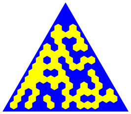
(a) Site percolation.

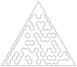
(b) $O(n)$ loop model. Percolation corresponds to $n=1$ and $x=1$, which is in the dense phase.

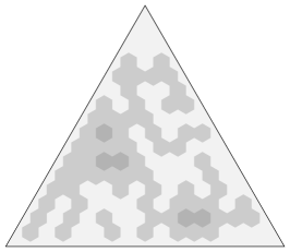
(c) Area shaded by nesting of loops.

Figure 1.1: Nesting of loops in the $O(n)$ loop model. Each $O(n)$ loop configuration has probability proportional to $x^{\text{total length of loops}}\times n^{\text{\# loops}}$. For a certain critical value of $x$, the $O(n)$ model for $0\leq n\leq 2$ has a “dilute phase”, which is believed to converge $\operatorname{CLE}_{\kappa}$ for $8/3<\kappa\leq 4$ with $n=-2\cos(4\pi/\kappa)$. For $x$ above this critical value, the $O(n)$ loop model is in a “dense phase”, which is believed to converge to $\operatorname{CLE}_{\kappa}$ for $4\leq\kappa\leq 8$, again with $n=-2\cos(4\pi/\kappa)$. See [KN04] for further background.

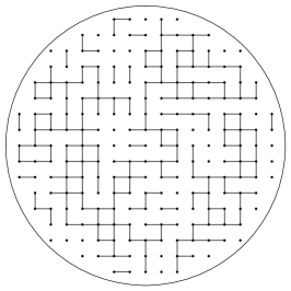
(a) Critical FK bond configuration. Here $q=2$.

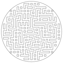
(b) Loops separating FK clusters from dual clusters.

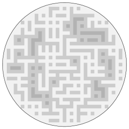
(c) Area shaded by nesting of loops.

Figure 1.2: Nesting of loops separating critical Fortuin-Kasteleyn (FK) clusters from dual clusters. Each FK bond configuration has probability proportional to $(p/(1-p))^{\text{\# edges}}\times q^{\text{\# clusters}}$ [FK72], where there is believed to be a critical point at $p=1/(1+1/\sqrt{q})$ (proved for $q\geq 1$ [BDC12]). For $0\leq q\leq 4$, these loops are believed to have the same large-scale behavior as the $O(n)$ model loops for $n=\sqrt{q}$ in the dense phase, that is, to converge to $\operatorname{CLE}_{\kappa}$ for $4\leq\kappa\leq 8$ (see [RS05, KN04]).

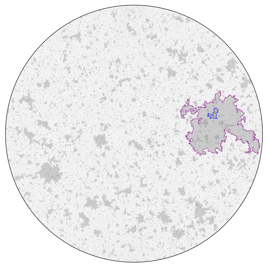
(a) $\operatorname{CLE}_{3}$ (from critical Ising model)

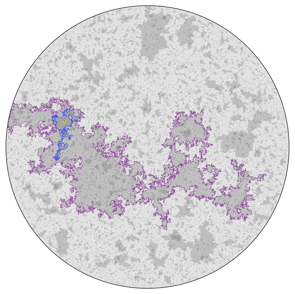
(b) $\operatorname{CLE}_{4}$ (from the FK model with $q=4$) $\star$

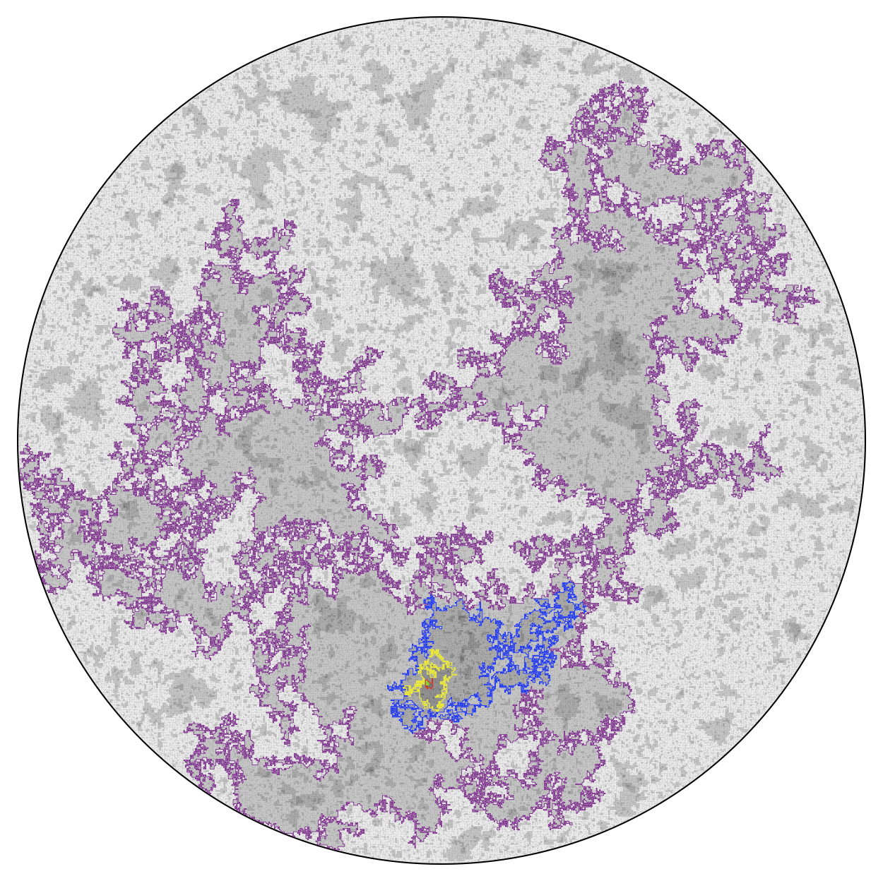
(c) $\operatorname{CLE}_{16/3}$ (from the FK model with $q=2$)

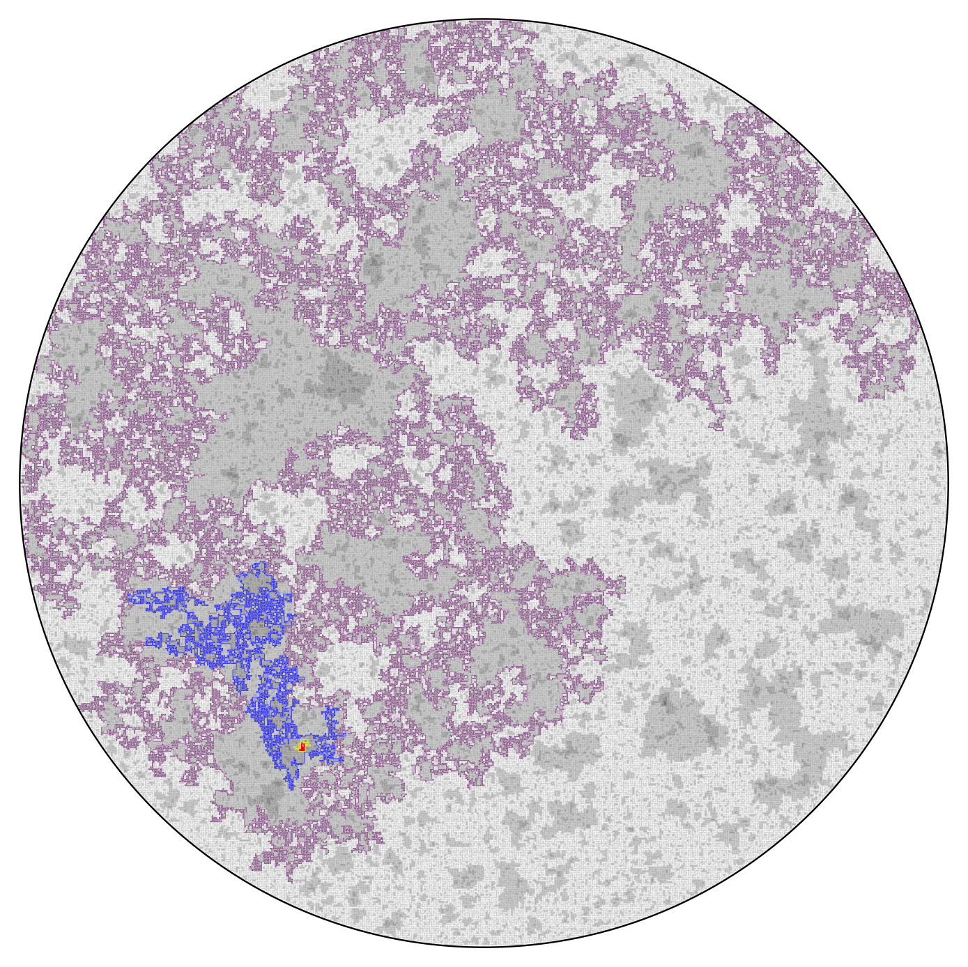
(d) $\operatorname{CLE}_{6}$ (from critical bond percolation) $\star$

Figure 1.3: Simulations of discrete loop models which converge to (or are believed to converge to, indicated with $\star$) $\operatorname{CLE}_{\kappa}$ in the fine mesh limit. For each of the $\operatorname{CLE}_{\kappa}$’s, one particular nested sequence of loops is outlined. For $\operatorname{CLE}_{\kappa}$, almost all of the points in the domain are surrounded by an infinite nested sequence of loops, though the discrete samples shown here display only a few orders of nesting.

Let $\kappa\in(8/3,8)$, let $D\subsetneq\mathbb{C}$ be a simply connected domain, and let $\Gamma$ be a $\operatorname{CLE}_{\kappa}$ in $D$. For each point $z\in D$ and $\varepsilon>0$, we let $\mathcal{N}_{z}(\varepsilon)$ be the number of loops of $\Gamma$ which surround $B(z,\varepsilon)$, the ball of radius $\varepsilon$ centered at $z$. We prove the existence and conformal invariance of the limit as $\varepsilon\to 0$ of the random function $z\mapsto\mathcal{N}_{z}(\varepsilon)-\mathbb{E}[\mathcal{N}_{z}(\varepsilon)]$ (with no additional normalization) in an appropriate space of distributions (Theorem 1.1). We refer to this object as the nesting field because, roughly, its value describes the fluctuations of the nesting of $\Gamma$ around its mean. This result also holds when the loops are assigned i.i.d. weights. More precisely, we fix a probability measure $\mu$ on $\mathbb{R}$ with finite second moment, define $\Gamma_{z}(\varepsilon)$ to be the set of loops in $\Gamma$ surrounding $B(z,\varepsilon)$, and define

$$\mathcal{S}_{z}(\varepsilon)=\sum_{\mathcal{L}\in\Gamma_{z}(\varepsilon)}\xi_{\mathcal{L}}\,,$$ (1.1)

where $\xi_{\mathcal{L}}$ are i.i.d. random variables with law $\mu$. We show that $z\mapsto\mathcal{S}_{z}(\varepsilon)-\mathbb{E}[\mathcal{S}_{z}(\varepsilon)]$ converges as $\varepsilon\to 0$ to a distribution we call the weighted nesting field. When $\kappa=4$ and $\mu$ is a signed Bernoulli distribution, the weighted nesting field is the GFF [MS14, MWW14]. Our result serves to generalize this construction to other values of $\kappa\in(8/3,8)$ and weight measures $\mu$. In Theorem 1.2, we answer a question asked in [She09, Problem 8.2].

The weighted nesting field is a random distribution, or generalized function, on $D$. Informally, it is too rough to be defined pointwise on $D$, but it is still possible to integrate it against sufficiently smooth compactly supported test functions on $D$. More precisely, we prove convergence to the nesting field in a certain local Sobolev space $H_{\operatorname{loc}}^{s}(D)\subset C_{c}^{\infty}(D)^{\prime}$ on $D$, where $C_{c}^{\infty}(D)$ is the space of compactly supported smooth functions on $D$, $C_{c}^{\infty}(D)^{\prime}$ is the space of distributions on $D$, and the index $s\in\mathbb{R}$ is a parameter characterizing how smooth the test functions need to be. We review all the relevant definitions in Section 5.

The nesting field gives a loop-free description of the conformal loop ensemble. For $\kappa\leq 4$ we believe that the nesting field determines the CLE, but that for $\kappa>4$ the CLE contains more information. (See Question 2 in the open problems section.) In order to prove the existence of the nesting field, we show that the law of CLE near a point rapidly forgets loops that are far away, in a sense that we make quantitative.

Given $h\in C_{c}^{\infty}(D)^{\prime}$ and $f\in C_{c}^{\infty}(D)$, we denote by $\langle h,f\rangle$ the evaluation of the linear functional $h$ at $f$. Recall that the pullback $h\circ\varphi^{-1}$ of $h\in C_{c}^{\infty}(D)^{\prime}$ under a conformal map $\varphi^{-1}$ is defined by $\langle h\circ\varphi^{-1},f\rangle\colonequals\langle h,|\varphi^{\prime}|^{2}f\circ\varphi\rangle$ for $f\in C_{c}^{\infty}(\varphi(D))$.

Theorem 1.1.

Fix $\kappa\in(8/3,8)$ and $\delta>0$, and suppose $\mu$ is a probability measure on $\mathbb{R}$ with finite second moment. Let $D\subsetneq\mathbb{C}$ be a simply connected domain. Let $\Gamma$ be a $\operatorname{CLE}_{\kappa}$ on $D$ and $(\xi_{\mathcal{L}})_{\mathcal{L}\in\Gamma}$ be i.i.d. weights on the loops of $\Gamma$ drawn from the distribution $\mu$. Recall that for $\varepsilon>0$ and $z\in D$, $\mathcal{S}_{z}(\varepsilon)$ denotes

$$\mathcal{S}_{z}(\varepsilon)=\sum_{\begin{subarray}{c}\mathcal{L}\in\Gamma\\ \text{$\mathcal{L}$ surrounds $B(z,\varepsilon)$}\end{subarray}}\xi_{\mathcal{L}}\,.$$

Let

$$h_{\varepsilon}(z)=\mathcal{S}_{z}(\varepsilon)-\mathbb{E}[\mathcal{S}_{z}(\varepsilon)]\,.$$ (1.2)

There exists an $H_{\operatorname{loc}}^{-2-\delta}(D)$-valued random variable $h=h(\Gamma,(\xi_{\mathcal{L}}))$ such that for all $f\in C_{c}^{\infty}(D)$, almost surely $\lim_{\varepsilon\to 0}\langle h_{\varepsilon},f\rangle=\langle h,f\rangle$. Moreover, $h(\Gamma,(\xi_{\mathcal{L}}))$ is almost surely a deterministic conformally invariant function of the CLE $\Gamma$ and the loop weights $(\xi_{\mathcal{L}})_{\mathcal{L}\in\Gamma}$: almost surely, for any conformal map $\varphi$ from $D$ to another simply connected domain, we have

$$h(\varphi(\Gamma),(\xi_{\varphi(\mathcal{L})})_{\mathcal{L}\in\Gamma})=h(\Gamma,(\xi_{\mathcal{L}})_{\mathcal{L}\in\Gamma})\circ\varphi^{-1}\,.$$

In Theorem 6.2, we prove a stronger form of convergence, namely almost sure convergence in the norm topology of $H^{-2-\delta}(D)$, when $\varepsilon$ tends to $0$ along any given geometric sequence.

We also consider the step nesting sequence, defined by

$$\mathfrak{h}_{n}(z)=\sum_{k=1}^{n}\xi_{\mathcal{L}_{k}(z)}-\mathbb{E}\left[\sum_{k=1}^{n}\xi_{\mathcal{L}_{k}(z)}\right],\quad n\in\mathbb{N},$$

where the random variables $(\xi_{\mathcal{L}})_{\mathcal{L}\in\Gamma}$ are i.i.d. with law $\mu$. We may assume without loss of generality that $\mu$ has zero mean, so that $\mathfrak{h}_{n}(z)=\sum_{k=1}^{n}\xi_{\mathcal{L}_{k}(z)}$. We establish the following convergence result for the step nesting sequence, which parallels Theorem 1.1:

Theorem 1.2.

Suppose that $D\subsetneq\mathbb{C}$ is a proper simply connected domain and $\delta>0$. Assume that the weight distribution $\mu$ has a finite second moment and zero mean. There exists an $H_{\operatorname{loc}}^{-2-\delta}(D)$-valued random variable $\mathfrak{h}$ such that $\lim_{n\to\infty}\mathfrak{h}_{n}=\mathfrak{h}$ almost surely in $H_{\operatorname{loc}}^{-2-\delta}(D)$. Moreover, $\mathfrak{h}$ is almost surely determined by $\Gamma$ and $(\xi_{\mathcal{L}})_{\mathcal{L}\in\Gamma}$.

Suppose that $\acute{D}$ is another simply connected domain and $\varphi\colon D\to\acute{D}$ is a conformal map. Let $\acute{h}$ be the random element of $H_{\operatorname{loc}}^{-2-\delta}(\acute{D})$ associated with the $\operatorname{CLE}$ $\acute{\Gamma}=\varphi(\Gamma)$ on $\acute{D}$ and weights $(\xi_{\varphi^{-1}(\acute{\mathcal{L}})})_{\acute{\mathcal{L}}\in\acute{\Gamma}}$. Then $\acute{\mathfrak{h}}=\mathfrak{h}\circ\varphi^{-1}$ almost surely.

In Proposition 7.2, we show that the step nesting field and the weighted nesting field are equal, under the assumption that $\mu$ has zero mean.

When $\kappa=4$, $\sigma=\sqrt{\pi/2}$, and $\mu=\mu_{B}$ where $\mu_{\rm B}(\{\sigma\})=\mu_{\rm B}(\{-\sigma\})=1/2$ (as in Theorem LABEL:I-thm::gff_maximum of [MWW14]) the distribution $h$ of Theorem 1.1 is that of a GFF on $D$ [MS14]. The existence of the distributional limit for other values of $\kappa$ was posed in [She09, Problem 8.2]. Note that in this context, $\tfrac{2}{\pi}\mathbb{E}[\mathcal{S}_{z}(\varepsilon)\mathcal{S}_{w}(\varepsilon)]$ is equal to the expected number of loops which surround both $B(z,\varepsilon)$ and $B(w,\varepsilon)$. Let $G_{D}(z,w)$ be the Green’s function for the negative Dirichlet Laplacian on $D$. Since $\mathcal{S}_{z}(\varepsilon)$ converges to the GFF [MS14], it follows that $\tfrac{2}{\pi}\mathbb{E}[\mathcal{S}_{z}(\varepsilon)\mathcal{S}_{w}(\varepsilon)]$ converges to $\frac{2}{\pi}G_{D}(z,w)$ (see Section 2 in [DPRZ01]). That is, the expected number of $\operatorname{CLE}_{4}$ loops which surround both $z$ and $w$ is given by $\frac{2}{\pi}G_{D}(z,w)$.

One of the elements of the proof of Theorem 1.1 is an extension of this bound which holds for all $\kappa\in(8/3,8)$. We include this as our final main theorem.

Theorem 1.3.

Let $\Gamma$ be a $\operatorname{CLE}_{\kappa}$ (with $8/3<\kappa<8$) on a simply connected proper domain $D$. For $z,w\in D$ distinct, let $\mathcal{N}_{z,w}$ be the number of loops of $\Gamma$ which surround both $z$ and $w$. For each integer $j\geq 1$, there exists a constant $C_{\kappa,j}\in(0,\infty)$ such that

$$\big{|}\mathbb{E}[\mathcal{N}_{z,w}^{j}]-(\nu_{\mathrm{typical}}\,2\pi\,G_{D}(z,w))^{j}\big{|}\leq C_{\kappa,j}(G_{D}(z,w)+1)^{j-1}\,.$$ (1.3)

Outline

In Section 2 we review background material and establish some general CLE estimates, and in Section 3 we prove Theorem 1.3. Section 4 includes proofs of several technical results used in the proof of Theorem 1.1. In Section 5 we provide a brief overview of the necessary material on distributions and Sobolev spaces, and we establish a general result (Proposition 5.1) regarding the almost-sure convergence of a sequence of random distributions. In Sections 6 and 7 we prove Theorems 1.1 and 1.2, respectively. We conclude by listing open questions in Section 8.

2 Basic CLE estimates

In this section we record some facts about CLE. We refer the reader to the preliminaries section in [MWW14] for an introduction to CLE. We begin by reminding the reader of the Koebe distortion theorem and the Koebe quarter theorem.

Theorem 2.1.

(Koebe distortion theorem) If $f:\mathbb{D}\to\mathbb{C}$ is an injective analytic function and $f(0)=0$, then

$$\frac{r}{(1+r)^{2}}|f^{\prime}(0)|\leq|f(re^{i\theta})|\leq\frac{r}{(1-r)^{2}}|f^{\prime}(0)|,\quad\text{for }\theta\in\mathbb{R}\text{ and }0\leq r<1\,.$$

The Koebe quarter theorem, which says that $B(0,\tfrac{1}{4}|f^{\prime}(0)|)\subset f(\mathbb{D})$, follows from the lower bound in the distortion theorem [Law05, Theorem 3.17]. Combining the quarter theorem with the Schwarz lemma [Law05, Lemma 2.1], we obtain the following corollary.

Corollary 2.2.

If $D\subsetneq\mathbb{C}$ is a simply connected domain, $z\in D$, and $f:\mathbb{D}\to D$ is a conformal map sending 0 to $z$, then the inradius $\operatorname{inrad}(z;D)\colonequals\inf_{w\in\mathbb{C}\setminus D}|z-w|$ and the conformal radius $\operatorname{CR}(z;D)\colonequals|f^{\prime}(0)|$ satisfy

$$\operatorname{inrad}(z;D)\leq\operatorname{CR}(z;D)\leq 4\,\operatorname{inrad}(z;D)\,.$$

For the $\operatorname{CLE}_{\kappa}$ $\Gamma$ in $D$, $z\in D$, and $j\geq 0$, we define $\mathcal{L}_{z}^{j}$ to be the $j$th outermost loop of $\Gamma$ which surrounds $z$. For $r>0$, we define

$$J^{\cap}_{z,r} \colonequals\min\{j\geq 1:\mathcal{L}_{z}^{j}\cap B(z,r)\neq\varnothing\}$$ (2.1a)

$$J^{\subset}_{z,r} \colonequals\min\{j\geq 1:\mathcal{L}_{z}^{j}\subset B(z,r)\}.$$ (2.1b)

Lemma 2.3.

For each $\kappa\in(8/3,8)$ there exists $p=p(\kappa)>0$ such that for any proper simply connected domain $D$ and $z\in D$,

$$\mathbb{P}[\mathcal{L}_{z}^{2}\subseteq B(z,\operatorname{dist}(z,\partial D))]\geq p.$$

Corollary 2.4.

$J^{\subset}_{z,r}-J^{\cap}_{z,r}$ is stochastically dominated by $2\widetilde{N}$ where $\widetilde{N}$ is a geometric random variable with parameter $p=p(\kappa)>0$ which depends only on $\kappa\in(8/3,8)$.

Proof.

See Corollary LABEL:I-cor::loop_contain_stoch_dom in [MWW14]. ∎

We use the following estimate for the overshoot of a random walk the first time it crosses a given threshold. We will apply this lemma to the random walk which tracks the negative log conformal radius of the sequence of CLE loops surrounding a given point $z\in D$, as viewed from $z$. See Lemma LABEL:I-lem::firsthitting in [MWW14] for a proof.

Lemma 2.5.

Suppose $\{X_{j}\}_{j\in\mathbb{N}}$ are nonnegative i.i.d. random variables for which $\mathbb{E}[X_{1}]>0$ and $\mathbb{E}[e^{\lambda_{0}X_{1}}]<\infty$ for some $\lambda_{0}>0$. Let $S_{n}=\sum_{j=1}^{n}X_{j}$ and $\tau_{x}=\inf\{n\geq 0:S_{n}\geq x\}$. Then there exists $C>0$ (depending on the law of $X_{1}$ and $\lambda_{0}$) such that $\mathbb{P}[S_{\tau_{x}}-x\geq\alpha]\leq C\exp(-\lambda_{0}\alpha)$ for all $x\geq 0$ and $\alpha>0$.

The following lemma provides a quantitative version of the statement that it is unlikely that there exists a CLE loop surrounding the inner boundary but not the outer boundary of a given small, thin annulus. We make use of a quantitative coupling between CLE in large domains and full-plane CLE, which appears as Theorem A.1 in the appendix.

Lemma 2.6.

Let $\Gamma$ be a $\operatorname{CLE}_{\kappa}$ in $\mathbb{D}$. There exist constants $C>0$, $\alpha>0$, and $\varepsilon_{0}>0$ depending only on $\kappa$ such that for $0<\varepsilon<\varepsilon_{0}$ and $0\leq\delta<1/2$,

$$\mathbb{E}[\mathcal{N}_{0}(\varepsilon(1-\delta))-\mathcal{N}_{0}(\varepsilon)]\leq C\delta+C\varepsilon^{\alpha}\,.$$ (2.2)

Proof.

We couple the $\operatorname{CLE}_{\kappa}$ $\Gamma_{\mathbb{D}}=\Gamma$ in the disk with a whole-plane $\operatorname{CLE}_{\kappa}$ $\Gamma_{\mathbb{C}}$ as in Theorem A.1. Index the loops of $\Gamma_{\mathbb{C}}$ surrounding $0$ by $\mathbb{Z}$ in such a way that $\mathcal{L}_{0}^{n}(\Gamma_{\mathbb{C}})$ and $\mathcal{L}_{0}^{n}(\Gamma_{\mathbb{D}})$ are exponentially close for large $n$. For $n\in\mathbb{N}$ define $V^{\mathbb{D}}_{n}=-\log\operatorname{inrad}\mathcal{L}_{0}^{n}(\Gamma_{\mathbb{D}})$, and for $n\in\mathbb{Z}$ define $V^{\mathbb{C}}_{n}=-\log\operatorname{inrad}\mathcal{L}_{0}^{n}(\Gamma_{\mathbb{C}})$. Since whole-plane $\operatorname{CLE}_{\kappa}$ is scale invariant, the set $\{V^{\mathbb{C}}_{n}\,:n\in\mathbb{Z}\}$ is translation invariant. Using Corollary 2.2 to compare $(V^{\mathbb{C}}_{n})_{n\in\mathbb{Z}}$ to the sequence of log conformal radii of the loops of $\Gamma_{\mathbb{C}}$ surrounding the origin, the translation invariance implies

$$\mathbb{E}\left[\#\left\{n\,:\,a\leq V^{\mathbb{C}}_{n}<b\right\}\right]=\nu_{\mathrm{typical}}(b-a)\,.$$

Let $\alpha$ and the term low distortion be defined as in the statement of Theorem A.1. With probability $1-O(\varepsilon^{\alpha})$ there is a low distortion map from $\Gamma_{\mathbb{D}}|_{B(0,\varepsilon)^{+}}$ to $\Gamma_{\mathbb{C}}|_{B(0,\varepsilon)^{+}}$, and on this event, we can bound

$$\#\left\{n\,:\,\log\frac{1}{\varepsilon}\leq V^{\mathbb{D}}_{n}<\log\frac{1}{\varepsilon(1-\delta)}\right\}\\ \leq\#\left\{n\,:\,\log\frac{1}{\varepsilon}-O(\varepsilon^{\alpha})\leq V^{\mathbb{C}}_{n}<\log\frac{1}{\varepsilon(1-\delta)}+O(\varepsilon^{\alpha})\right\}\,.$$

On the event that there is no such low distortion map, this can be detected by comparing the boundaries of $\Gamma_{\mathbb{D}}|_{B(0,\varepsilon)^{+}}$ and $\Gamma_{\mathbb{C}}|_{B(0,\varepsilon)^{+}}$, so that conditional on this unlikely event, $\Gamma_{\mathbb{D}}|_{B(0,\varepsilon)^{+}}$ is still an unbiased $\operatorname{CLE}_{\kappa}$ conformally mapped to the region surrounded by the boundary of $\Gamma_{\mathbb{D}}|_{B(0,\varepsilon)^{+}}$. In particular, the sequence of log-conformal radii of loops of $\Gamma_{\mathbb{D}}|_{B(0,\varepsilon)^{+}}$ surrounding $0$ is a renewal process, which together with the Koebe distortion theorem and the bound $\delta\leq 1/2$ imply

$$\mathbb{E}[\mathcal{N}_{0}(\varepsilon(1-\delta))-\mathcal{N}_{0}(\varepsilon)\,|\,\text{no low distortion map}]\leq\text{constant}\,.$$

Combining these bounds yields (2.2). ∎

Lemma 2.7.

For each $\kappa\in(8/3,8)$ and integer $j\in\mathbb{N}$, there are constants $C>0$, $\alpha>0$, and $\varepsilon_{0}>0$ (depending only on $\kappa$ and $j$) such that whenever $D$ is a simply connected proper domain, $z\in D$, $\varphi$ is a conformal transformation of $D$, and $0<\varepsilon<\varepsilon_{0}$, if $\Gamma$ is a $\operatorname{CLE}_{\kappa}$ in $D$, then

$$\mathbb{E}\bigg{[}\big{|}\mathcal{N}_{z}(\varepsilon\operatorname{CR}(z;D);\Gamma)-\mathcal{N}_{\varphi(z)}(\varepsilon\operatorname{CR}(\varphi(z);\varphi(D));\varphi(\Gamma))\big{|}^{j}\bigg{]}\leq C\varepsilon^{\alpha}\,.$$

Proof.

Observe that translating and scaling the domain $D$ or its conformal image $\varphi(D)$ has no effect on the loop counts, so we assume without loss of generality that $z=0$, $\varphi(z)=0$, $\operatorname{CR}(z;D)=1$, and $\operatorname{CR}(\varphi(z);\varphi(D))=1$. Observe also that it suffices to prove this lemma in the case that the domain $D$ is the unit disk $\mathbb{D}$, since a general $\varphi$ may be expressed as the composition $\varphi=\varphi_{2}\circ\varphi_{1}^{-1}$ where $\varphi_{1}$ and $\varphi_{2}$ are conformal transformations of the unit disk with $\varphi_{i}(0)=0$ and $\varphi_{i}^{\prime}(0)=1$, and the desired bound follows from the triangle inequality.

Let $\Gamma$ be a $\operatorname{CLE}_{\kappa}$ on $\mathbb{D}$, and let $\acute{\Gamma}=\varphi(\Gamma)$. By the Koebe distortion theorem and the elementary inequality

$$1-3r\leq\frac{1}{(1+r)^{2}}\leq\frac{1}{(1-r)^{2}}\leq 1+3r,\quad\text{for $r$ small enough},$$ (2.3)

we have

$$B(0,\varepsilon-3\varepsilon^{2})\subset\varphi^{-1}(B(0,\varepsilon))\subset B(0,\varepsilon+3\varepsilon^{2})\,,$$

for small enough $\varepsilon$. Hence $\mathcal{N}_{0}(\varepsilon+3\varepsilon^{2};\Gamma)\leq\mathcal{N}_{0}(\varepsilon;\acute{\Gamma})\leq\mathcal{N}_{0}(\varepsilon-3\varepsilon^{2};\Gamma)$, and so for

$$X\colonequals\mathcal{N}_{0}(\varepsilon-3\varepsilon^{2};\Gamma)-\mathcal{N}_{0}(\varepsilon+3\varepsilon^{2};\Gamma)$$

we have $|\mathcal{N}_{0}(\varepsilon;\acute{\Gamma})-\mathcal{N}_{0}(\varepsilon;\Gamma)|\leq X$.

By Lemma 2.6 we have $\mathbb{E}[X]=O(\varepsilon^{\alpha})$, which proves the case $j=1$.

Notice that the conformal radius of every new loop after the first that intersects $B(0,\varepsilon+3\varepsilon^{2})$ has a uniformly positive probability of being less than $\frac{1}{4}(\varepsilon-3\varepsilon^{2})$, conditioned on the previous loop. By the Koebe quarter theorem, such a loop intersects $B(0,\varepsilon-3\varepsilon^{2})$. Thus for some $p<1$ we have $\mathbb{P}[X\geq k+1]\leq p\mathbb{P}[X\geq k]$ for $k\geq 0$. Hence

$$\mathbb{E}[X^{j}]=\sum_{k=1}^{\infty}k^{j}\mathbb{P}[X=k] \leq\sum_{k=1}^{\infty}k^{j}p^{k}\mathbb{P}[X=1]\leq\left(\sum_{k=1}^{\infty}k^{j}p^{k}\right)\mathbb{E}[X]=O(\varepsilon^{\alpha})\,,$$

which proves the cases $j>1$. ∎

3 Co-nesting estimates

We use the following lemma in the proof of Theorem 1.3:

Lemma 3.1.

Let $\lambda_{0}>0$, and suppose $\{X_{j}\}_{j\in\mathbb{N}}$ are nonnegative i.i.d. random variables for which $\mathbb{E}[X_{1}]>0$ and $\mathbb{E}[e^{\lambda_{0}X_{1}}]<\infty$. Let $\Lambda(\lambda)=\log\mathbb{E}[e^{\lambda X_{1}}]$ and let $S_{n}=\sum_{j=1}^{n}X_{j}$. For $x>0$, define $\tau_{x}=\inf\{n\geq 0:S_{n}\geq x\}$. For $\lambda<\lambda_{0}$, let

$$M_{n}^{\lambda}=\exp(\lambda S_{n}-\Lambda(\lambda)n).$$

Then for $\lambda<\lambda_{0}$ and $x\geq 0$, the random variables $\{M_{n\wedge\tau_{x}}^{\lambda}\}_{n\in\mathbb{N}}$ are uniformly integrable.

Proof.

Fix $\beta>1$ such that $\beta\lambda<\lambda_{0}$. By Hölder’s inequality, any family of random variables which is uniformly bounded in $L^{p}$ for some $p>1$ is uniformly integrable. Therefore, it suffices to show that $\sup_{n\geq 0}\mathbb{E}[(M_{n\wedge\tau_{x}}^{\lambda})^{\beta}]<\infty$. We have,

$$(M_{n\wedge\tau_{x}}^{\lambda})^{\beta} =\exp(\beta\lambda(S_{n\wedge\tau_{x}}-x))\times\exp(\beta\lambda x-\beta\Lambda(\lambda)(n\wedge\tau_{x}))$$

$$\leq\exp(\beta\lambda(S_{\tau_{x}}-x))\times\exp(\beta\lambda x).$$

The result follows from Lemma 2.5. ∎

Proof of Theorem 1.3.

Fix $z,w\in D$ distinct and $j\in\mathbb{N}$. Let $\varphi\colon D\to\mathbb{D}$ be the conformal map which sends $z$ to $0$ and $w$ to $e^{-x}\in(0,1)$. Let $G_{D}$ (resp. $G_{\mathbb{D}}$) be the Green’s function for $-\Delta$ with Dirichlet boundary conditions on $D$ (resp. $\mathbb{D}$). Explicitly,

$$G_{\mathbb{D}}(u,v)=\frac{1}{2\pi}\log\frac{|1-\overline{u}v|}{|u-v|}\quad\text{for}\quad u,v\in\mathbb{D}.$$

In particular, $G_{\mathbb{D}}(0,u)=\frac{1}{2\pi}\log|u|^{-1}$ for $u\in\mathbb{D}$. By the conformal invariance of $\operatorname{CLE}_{\kappa}$ and the Green’s function, i.e. $G_{D}(u,v)=G_{\mathbb{D}}(\varphi(u),\varphi(v))$, it suffices to show that there exists a constant $C_{j,\kappa}\in(0,\infty)$ which depends only on $j$ and $\kappa\in(8/3,8)$ such that

$$\big{|}\mathbb{E}[(\mathcal{N}_{0,e^{-x}})^{j}]-(\nu_{\mathrm{typical}}x)^{j}\big{|}\leq C_{j,\kappa}(x+1)^{j-1}\quad\quad\text{for all $x>0$}.$$ (3.1)

Let $\{T_{i}\}_{i\in\mathbb{N}}$ be the sequence of $\log$ conformal radii increments associated with the loops of $\Gamma$ which surround $0$, let $S_{k}=\sum_{i=1}^{k}T_{i}$, and let $\tau_{x}=\min\{k\geq 1:S_{k}\geq x\}$. Recall that $\Lambda_{\kappa}(\lambda)$ denotes the $\log$ moment generating function of the law of $T_{1}$. Let $M_{n}=\exp(\lambda S_{n}-\Lambda_{\kappa}(\lambda)n)$. By Lemma 3.1, $\{M_{n\wedge\tau_{x}}\}_{n\in\mathbb{N}}$ is a uniformly integrable martingale for $\lambda<1-\tfrac{2}{\kappa}-\tfrac{3\kappa}{32}$. By Lemma 2.5, we can write $S_{\tau_{x}}=x+X$ where $\mathbb{E}[e^{\lambda X}]<\infty$. By the optional stopping theorem for uniformly integrable martingales (see [Wil91, § A14.3]), we have that

$$1=\mathbb{E}[\exp(\lambda S_{\tau_{x}}-\Lambda_{\kappa}(\lambda)\tau_{x})]=\mathbb{E}[\exp(\lambda x+\lambda X-\Lambda_{\kappa}(\lambda)\tau_{x})].$$ (3.2)

We argue by induction on $j$ that

$$\mathbb{E}[(\Lambda^{\prime}_{\kappa}(0)\tau_{x})^{j}]=x^{j}+O((x+1)^{j-1}).$$ (3.3)

The base case $j=0$ is trivial.

If we differentiate (3.2) with respect to $\lambda$ and then evaluate at $\lambda=0$, we obtain

$$0=\mathbb{E}[(x+X-\Lambda^{\prime}_{\kappa}(0)\tau_{x})].$$

If we instead differentiate twice, we obtain

$$0=\mathbb{E}[(x+X-\Lambda^{\prime}_{\kappa}(0)\tau_{x})^{2}-\Lambda^{\prime\prime}_{\kappa}(0)\tau_{x}].$$

Similarly, if we differentiate $j$ times with respect to $\lambda$ and then evaluate at $\lambda=0$, we obtain

$$0=\mathbb{E}[(x+X-\Lambda^{\prime}_{\kappa}(0)\tau_{x})^{j}]+\sum_{\begin{subarray}{c}i\geq 0,k\geq 1\\ i+2k\leq j\end{subarray}}A_{\kappa,i,k}\mathbb{E}[(x+X-\Lambda^{\prime}_{\kappa}(0)\tau_{x})^{i}\tau_{x}^{k}],$$ (3.4)

where the $A_{\kappa,i,k}$’s are constant coefficients depending on the higher order derivatives of $\Lambda_{\kappa}$ at $0$. By our induction hypothesis, for $h<j$ we have $\mathbb{E}[\tau_{x}^{h}]=O((x+1)^{h})$. Conditional on $\tau_{x}$, $X$ has exponentially small tails, so $\mathbb{E}[\tau_{x}^{h}X^{\ell}]=O((x+1)^{h})$ as well. From this we obtain

$$0=\mathbb{E}[(x-\Lambda^{\prime}_{\kappa}(0)\tau_{x})^{j}]+O((x+1)^{j-1}).$$ (3.5)

Using our induction hypothesis again for $h<j$, we obtain

$$0=\sum_{h=0}^{j-1}\binom{j}{h}(-1)^{h}x^{j}+\mathbb{E}[(-\Lambda^{\prime}_{\kappa}(0)\tau_{x})^{j}]+O((x+1)^{j-1}),$$ (3.6)

from which (3.3) follows, completing the induction.

Recall that $J_{0,r}^{\cap}$ (resp. $J_{0,r}^{\subset}$) is the smallest index $j$ such that $\mathcal{L}_{0}^{j}$ intersects (resp. is contained in) $B(0,r)$. It is straightforward that

$$\tau_{x-\log 4}\leq J_{0,e^{-x}}^{\cap}\leq\mathcal{N}_{0,e^{-x}}+1\leq J_{0,e^{-x}}^{\subset}.$$

Since the $\tau$’s are stopping times for an i.i.d. sum, conditional on the value of $\tau_{x-\log 4}$, the difference $\tau_{x}-\tau_{x-\log 4}$ has exponentially decaying tails. Moreover, by Lemma 2.3, conditional on the value of $\tau_{x}$, $J_{0,e^{-x}}^{\subset}-\tau_{x}$ has exponentially decaying tails. Thus $\mathbb{E}[\mathcal{N}_{0,e^{-x}}^{j}]=\mathbb{E}[\tau_{x}^{j}]+O((x+1)^{j-1})$. Finally, we recall that $1/\Lambda_{\kappa}^{\prime}(0)=1/\mathbb{E}[T_{1}]=\nu_{\mathrm{typical}}$. ∎

By combining Theorem 1.3 and Corollary 2.4, we can estimate the moments of the number of loops which surround a ball in terms of powers of $G_{D}(z,w)$.

Corollary 3.2.

There exists a constant $C_{j,\kappa}\in(0,\infty)$ depending only on $\kappa\in(8/3,8)$ and $j\in\mathbb{N}$ such that the following is true. For each $\varepsilon>0$ and $z\in D$ for which $\operatorname{dist}(z,\partial D)\geq 2\varepsilon$ and $\theta\in\mathbb{R}$, we have

$$\big{|}\mathbb{E}[(\mathcal{N}_{z}(\varepsilon))^{j}]-(2\pi\nu_{\mathrm{typical}}G_{D}(z,z+\varepsilon e^{i\theta}))^{j}\big{|}\leq C_{j,\kappa}(G_{D}(z,z+\varepsilon e^{i\theta})+1)^{j-1}.$$ (3.7)

In particular, there exists constant a constant $C_{\kappa}\in(0,\infty)$ depending only on $\kappa\in(8/3,8)$ such that

$$\left|\mathbb{E}[\mathcal{N}_{z}(\varepsilon)]-\nu_{\mathrm{typical}}\log\frac{\operatorname{CR}(z;D)}{\varepsilon}\right|\leq C_{\kappa}\,.$$ (3.8)

Proof.

Let $w=z+\varepsilon e^{i\theta}$. Corollary 2.4 implies that $|\mathcal{N}_{z,w}-\mathcal{N}_{z}(\varepsilon)|$ is stochastically dominated by a geometric random variable whose parameter $p$ depends only on $\kappa$. Consequently, (3.7) is a consequence of Theorem 1.3. To see (3.8), we apply (3.7) for $j=1$ and use that $G_{D}(u,v)=\tfrac{1}{2\pi}\log|u-v|^{-1}-\psi_{u}(v)$ where $\psi_{u}(v)$ is the harmonic extension of $v\mapsto\tfrac{1}{2\pi}\log|u-v|^{-1}$ from $\partial D$ to $D$. In particular, $\psi_{z}(z)=\tfrac{1}{2\pi}\log\operatorname{CR}(z;D)$. ∎

4 Regularity of the $\varepsilon$-ball nesting field

A key estimate that we use in the proof of Theorem 1.1 is the following bound on how much the centered nesting field $h_{\varepsilon}$ depends on $\varepsilon$. The proof of Theorem 4.1 and the remaining sections may be read in either order.

Theorem 4.1.

Let $D$ be a proper simply connected domain, and let $h_{\varepsilon}(z)$ be the centered weighted nesting around the ball $B(z,\varepsilon)$ of a $\operatorname{CLE}_{\kappa}$ on $D$, defined in (1.2). Suppose $0<\varepsilon_{1}(z)\leq\varepsilon$ and $0<\varepsilon_{2}(z)\leq\varepsilon$ on a compact subset $K\subset D$ of the domain. Then there is some $c>0$ (depending on $\kappa$) and $C_{0}>0$ (depending on $\kappa$, $D$, $K$, and the loop weight distribution) for which

$$\iint\limits_{K\times K}\big{|}\mathbb{E}\big{[}(h_{\varepsilon_{1}(z)}(z){-}h_{\varepsilon_{2}(z)}(z))\,(h_{\varepsilon_{1}(w)}(w){-}h_{\varepsilon_{2}(w)}(w))\big{]}\big{|}\,dz\,dw\leq C_{0}\varepsilon^{c}\,.$$ (4.1)

Proof.

Let $A$, $B$, and $C$ be the disjoint sets of loops for which $A\cup B$ is the set of loops surrounding $B(z,\varepsilon_{1}(z))$ or $B(z,\varepsilon_{2}(z))$ but not both, and $B\cup C$ is the set of loops surrounding $B(w,\varepsilon_{1}(w))$ or $B(w,\varepsilon_{2}(w))$ but not both. Letting $\xi_{\mathcal{L}}$ denote the weight of loop $\mathcal{L}$, then we have

$$\mathbb{E}[(h_{\varepsilon_{1}(z)} (z){-}h_{\varepsilon_{2}(z)}(z))(h_{\varepsilon_{1}(w)}(w){-}h_{\varepsilon_{2}(w)}(w))]$$

$$=\operatorname{Cov}[h_{\varepsilon_{1}(z)}(z){-}h_{\varepsilon_{2}(z)}(z),h_{\varepsilon_{1}(w)}(w)-h_{\varepsilon_{2}(w)}(w)]$$

$$=\pm\operatorname{Cov}\left[\sum_{a\in A}\xi_{a}+\sum_{b\in B}\xi_{b},\sum_{b\in B}\xi_{b}+\sum_{c\in C}\xi_{c}\right]$$ (4.2)

$$=\pm\operatorname{Var}[\xi]\,\mathbb{E}[|B|]\,\pm\mathbb{E}[\xi]^{2}\operatorname{Cov}[|A|{+}|B|,|B|{+}|C|]$$

$$=\pm\operatorname{Var}[\xi]\,\mathbb{E}[|B|]\,+\mathbb{E}[\xi]^{2}\operatorname{Cov}(\mathcal{N}_{z}(\varepsilon_{1}){-}\mathcal{N}_{z}(\varepsilon_{2}),\mathcal{N}_{w}(\varepsilon_{1}){-}\mathcal{N}_{w}(\varepsilon_{2}))\,,$$

where the $\pm$ signs are the sign of $(\varepsilon_{1}(z){-}\varepsilon_{2}(z))(\varepsilon_{1}(w){-}\varepsilon_{2}(w))$.

Let $G_{D}^{\kappa,\varepsilon}(z,w)$ denote the expected number of loops surrounding $z$ and $w$ but surrounding neither $B(z,\varepsilon)$ nor $B(w,\varepsilon)$. Then $\mathbb{E}[|B|]\leq G_{D}^{\kappa,\varepsilon}(z,w)$. In Lemma 4.3 we prove

$$\iint_{K\times K}G_{D}^{\kappa,\varepsilon}(z,w)\,dz\,dw\leq C_{1}\varepsilon^{c}\,,$$

and in Lemma 4.8 we prove

$$\iint_{K\times K}\big{|}\operatorname{Cov}(\mathcal{N}_{z}(\varepsilon_{1}(z))-\mathcal{N}_{z}(\varepsilon_{2}(z)),\mathcal{N}_{w}(\varepsilon_{1}(w))-\mathcal{N}_{w}(\varepsilon_{2}(w)))\big{|}\,dz\,dw\leq C_{2}\varepsilon^{c}\,,$$

where $c$ depends only on $\kappa$ and $C_{1}$ and $C_{2}$ depend only on $\kappa$, $D$, and $K$. Equation (4.1) follows from these bounds. ∎

In the remainder of this section we prove Lemmas 4.3 and 4.8.

Lemma 4.2.

For any $\kappa\in(8/3,8)$ and $j\in\mathbb{N}$, there is a positive constant $c>0$ such that, whenever $D\subsetneq\mathbb{C}$ is a simply connected proper domain, $z\in D$, and $0<\varepsilon<r$, the $j^{\text{th}}$ moment of the number of $\operatorname{CLE}_{\kappa}$ loops surrounding $z$ which intersect $B(z,\varepsilon)$ but are not contained in $B(z,r)$ is $O((\varepsilon/r)^{c})$.

Proof.

If there is a loop $\mathcal{L}=\mathcal{L}_{z}^{k}$ surrounding $z$ which is not contained in $B(z,r)$ and comes within distance $\varepsilon$ of $z$, then $J_{z,\varepsilon}^{\cap}\leq k$ and $J_{z,r}^{\subset}>k$, so $J_{z,\varepsilon}^{\cap}<J_{z,r}^{\subset}$. But from Corollary 2.4 $J_{z,r}^{\subset}-J_{z,r}^{\cap}$ is dominated by twice a geometric random variable, and by Lemma LABEL:I-lem::firsthitting in [MWW14] together with the Koebe quarter theorem we have $J_{z,\varepsilon}^{\cap}-J_{z,r}^{\cap}$ is order $\log(r/\varepsilon)$ except with probability $O((\varepsilon/r)^{c_{1}})$, for some constant $c_{1}>0$ (depending on $\kappa$). Therefore, except with probability $O((\varepsilon/r)^{c_{2}})$ (with $c_{2}=c_{2}(\kappa)>0$), we have $J_{z,\varepsilon}^{\cap}\geq J_{z,r}^{\subset}$. In this case there is no loop $\mathcal{L}$ surrounding $z$, not contained in $B(z,r)$, and coming within distance $\varepsilon$ of $z$. Finally, note that conditioned on the event that there is such a loop $\mathcal{L}$, the conditional expected number of such loops is by Corollary 2.4 dominated by twice a geometric random variable. ∎

Lemma 4.3.

For some positive constant $c<2$,

$$\iint_{K\times K}G_{D}^{\kappa,\varepsilon}(z,w)\,dz\,dw=O(\operatorname{area}(K)^{2-c/2}\varepsilon^{c})\,.$$ (4.3)

Proof.

Let $F^{\varepsilon}_{z,w}$ denote the number of loops surrounding both $z$ and $w$ but not $B(z,\varepsilon)$ or $B(w,\varepsilon)$. Then $G_{D}^{\kappa,\varepsilon}(z,w)=\mathbb{E}[F^{\varepsilon}_{z,w}]$.

Suppose $|z-w|\leq\varepsilon$. Let $\mathcal{L}$ be the outermost loop (if any) surrounding both $z$ and $w$ but not $B(z,\varepsilon)$ or $B(w,\varepsilon)$. The number of additional such loops is $\mathcal{N}_{z,w}(\Gamma^{\prime})$, where $\Gamma^{\prime}$ is a $\operatorname{CLE}_{\kappa}$ in $\operatorname{int}\mathcal{L}$, and by Theorem 1.3 we have $\mathbb{E}[\mathcal{N}_{z,w}(\Gamma^{\prime})]\leq C_{1}\log(\varepsilon/|z-w|)+C_{2}$ for some constants $C_{1}$ and $C_{2}$. Integrating the logarithm, we find that

$$\iint_{\begin{subarray}{c}K\times K\\ |z-w|\leq\varepsilon\end{subarray}}G_{D}^{\kappa,\varepsilon}(z,w)\,dz\,dw=O(\operatorname{area}(K)\varepsilon^{2})\,.$$ (4.4)

Next suppose $|z-w|>\varepsilon$. Now $F^{\varepsilon}_{z,w}$ is dominated by the number of loops surrounding $z$ which intersect $B(z,\varepsilon)$ but are not contained in $B(z,|z-w|)$, and Lemma 4.2 bounds the expected number of these loops by $O((\varepsilon/|z-w|)^{c})$ for some $c>0$. We decrease $c$ if necessary to ensure $0<c<2$, and let $R=\operatorname{area}(K)^{1/2}$. Since $(\varepsilon/|z-w|)^{c}$ is decreasing in $|z-w|$, we can bound

$$\iint_{\begin{subarray}{c}K\times K\\ |z-w|>\varepsilon\end{subarray}}G_{D}^{\kappa,\varepsilon}(z,w)\,dz\,dw \leq\iint_{\begin{subarray}{c}R\mathbb{D}\times R\mathbb{D}\\ |z-w|>\varepsilon\end{subarray}}O((\varepsilon/|z-w|)^{c})\,dz\,dw$$

$$=O(\operatorname{area}(K)^{2-c/2}\varepsilon^{c})\,.$$ (4.5)

Combining (4.4) and (4.5), using again $c<2$, we obtain (4.3). ∎

We let $S_{z,w}$ be the index of the outermost loop surrounding $z$ which separates $z$ from $w$ in the sense that $w\notin U_{z}^{S_{z,w}}$. Note that $S_{z,w}$ is also the smallest index for which $z\notin U_{w}^{S_{z,w}}$:

$$S_{z,w}\colonequals\min\{k:w\notin U_{z}^{k}\}=\min\{k:z\notin U_{w}^{k}\}\,.$$ (4.6)

We let $\Sigma_{z,w}$ denote the $\sigma$-algebra

$$\Sigma_{z,w}\colonequals\sigma(\{\mathcal{L}_{z}^{k}\,:1\leq k\leq S_{z,w}\}\cup\{\mathcal{L}_{w}^{k}\,:1\leq k\leq S_{z,w}\})\,.$$ (4.7)

Lemma 4.4.

There is a constant $C$ (depending only on $\kappa$) such that if $z,w\in D$ are distinct, then

$$-C\leq\mathbb{E}\!\left[\log\frac{\operatorname{CR}(z;U_{z}^{S_{z,w}})}{\min(|z-w|,\operatorname{CR}(z;D))}\right]\leq C\,.$$

Proof.

Let $r=\min(|z-w|,\operatorname{dist}(z,\partial D))$. By the Koebe distortion theorem, $\operatorname{CR}(z;U_{z}^{S_{z,w}})\leq 4r$, which gives the upper bound. By [MWW14, Lemma LABEL:I-lem::annulus-loop], there is a loop contained in $B(z,r)$ but which surrounds $B(z,r/2^{k})$ except with probability exponentially small $k$, which gives the lower bound. ∎

Lemma 4.5.

There exists a constant $C>0$ (depending only on $\kappa$) such that if $z,w\in D$ are distinct, and $0<\varepsilon<\min(|z-w|,\operatorname{CR}(z;D))$, then on the event $\{\operatorname{CR}(z;U_{z}^{S_{z,w}})\geq 8\varepsilon\}$,

$$\bigg{|}\mathbb{E}\big{[}J^{\cap}_{z,\varepsilon}-S_{z,w}\,|\,U_{z}^{S_{z,w}}\big{]}-\mathbb{E}\big{[}J^{\cap}_{z,\varepsilon}-S_{z,w}\big{]}-\\ \nu_{\mathrm{typical}}\log\frac{\operatorname{CR}(z;U_{z}^{S_{z,w}})}{\min(|z-w|,\operatorname{CR}(z;D))}\bigg{|}\leq C\,.$$ (4.8)

Proof.

Let $S=S_{z,w}$. By (3.8) of Corollary 3.2 we see that there exist $C_{1}>0$ such that on the event $\{\operatorname{CR}(z;U_{z}^{S})\geq 8\varepsilon\}$ we have

$$\left|\mathbb{E}\big{[}J_{z,\varepsilon}^{\cap}-S_{z,w}\,|\,U_{z}^{S_{z,w}}\big{]}-\nu_{\mathrm{typical}}\log\frac{\operatorname{CR}\big{(}z;U_{z}^{S_{z,w}}\big{)}}{\varepsilon}\right|\leq C_{1}\,.$$ (4.9)

We can write

$$\mathbb{E}\left[J_{z,\varepsilon}^{\cap}-S\right] =\mathbb{E}\left[(J_{z,\varepsilon}^{\cap}-S){\bf 1}_{\{\operatorname{CR}(z;U_{z}^{S})\geq 8\varepsilon\}}\right]+\mathbb{E}\left[(J_{z,\varepsilon}^{\cap}-S){\bf 1}_{\{\operatorname{CR}(z;U_{z}^{S})<8\varepsilon\}}\right]\,.$$ (4.10)

Applying (4.9), we can write the first term of (4.10) as,

$$\mathbb{E}\left[(J_{z,\varepsilon}^{\cap}-S){\bf 1}_{\{\operatorname{CR}(z;U_{z}^{S})\geq 8\varepsilon\}}\right] =\mathbb{E}\!\left[\mathbb{E}[J_{z,\varepsilon}^{\cap}-S\,|\,U_{z}^{S}]\,{\bf 1}_{\{\operatorname{CR}(z;U_{z}^{S})\geq 8\varepsilon\}}\right]$$

$$=\mathbb{E}\!\left[\left(\nu_{\mathrm{typical}}\log\frac{\operatorname{CR}(z;U_{z}^{S})}{\varepsilon}\pm C_{1}\right){\bf 1}_{\{\operatorname{CR}(z;U_{z}^{S})\geq 8\varepsilon\}}\right]$$

$$=\nu_{\mathrm{typical}}\log\frac{\min(|z-w|,\operatorname{CR}(z;D))}{\varepsilon}\pm\text{const}$$

$$\quad-\mathbb{E}\!\left[\left(\nu_{\mathrm{typical}}\log\frac{\operatorname{CR}(z;U_{z}^{S})}{\varepsilon}\right){\bf 1}_{\{\operatorname{CR}(z;U_{z}^{S})<8\varepsilon\}}\right]\,.$$

Using [MWW14, Lemma LABEL:I-lem::annulus-loop], there is a loop contained in $B(z,\varepsilon)$ which surrounds $B(z,\varepsilon/2^{k})$ except with probability exponentially small in $k$, so the last term on the right is bounded by a constant (depending on $\kappa$).

If $J_{z,\varepsilon}^{\cap}\geq S$, then $J_{z,\varepsilon}^{\cap}-S$ counts the number of loops $(\mathcal{L}_{z}^{k})_{k\in\mathbb{N}}$ after separating $z$ from $w$ before hitting $B(z,\varepsilon)$. If $J_{z,\varepsilon}^{\cap}\leq S$, then $S-J_{z,\varepsilon}^{\cap}$ counts the number of loops $(\mathcal{L}_{z}^{k})_{k\in\mathbb{N}}$ after intersecting $B(z,\varepsilon)$ before separating $z$ from $w$. Consequently, by Corollary 2.4, we see that absolute value of the second term of (4.10) is bounded by some constant $C_{2}>0$. Putting these two terms of (4.10) together, we obtain

$$\left|\mathbb{E}\left[J_{z,\varepsilon}^{\cap}-S_{z,w}\right]-\nu_{\mathrm{typical}}\log\frac{\min(|z-w|,\operatorname{CR}(z;D))}{\varepsilon}\right|\leq\text{const}\,.$$ (4.11)

Subtracting (4.11) from (4.9) and rearranging gives (4.8). ∎

Lemma 4.6.

Let $\{X_{j}\}_{j\in\mathbb{N}}$ be non-negative i.i.d. random variables whose law has a positive density with respect to Lebesgue measure on $(0,\infty)$ and for which there exists $\lambda_{0}>0$ such that $\mathbb{E}[e^{\lambda_{0}X_{1}}]<\infty$. For $a\geq 0$, let $S^{a}_{n}=a+\sum_{j=1}^{n}X_{j}$, and for $a,M>0$, let $\tau^{a}_{M}=\min\{n\geq 0:S^{a}_{n}\geq M\}$. There exists a coupling between $S^{a}$ and $\widehat{S}^{b}$ (identically distributed to $S^{b}$ but not independent of it) and constants $C,c>0$ so that for all $0\leq a\leq b\leq M$, we have

$$\mathbb{P}\bigg{[}S^{a}_{\tau^{a}_{M}}=\widehat{S}^{b}_{\widehat{\tau}^{b}_{M}}\bigg{]}\geq 1-Ce^{-cM}.$$

Similar but non-quantitative convergence results are known for more general distributions (for example, see [Gut09, Chapt. 3.10]). For our results we need this convergence to be exponentially fast, for which we did not find a proof, so we provide one.

Proof of Lemma 4.6.

For $M>N>0$, we construct a coupling between $\rho_{N}$ and $\rho_{M}$ as follows. We take $S_{0}=0$ and $\widehat{S}_{0}=N-M$, and then take $\{X_{j}\}_{j\in\mathbb{N}}$ and $\{\widehat{X}_{j}\}_{j\in\mathbb{N}}$ to be two i.i.d. sequences with law as in the statement of the lemma, with the two sequences coupled with one another in a manner that we shall describe momentarily. We let $S_{n}=\sum_{i=1}^{n}X_{i}$ and $\widehat{S}_{n}=\widehat{S}_{0}+\sum_{i=1}^{n}\widehat{X}_{i}$. Define stopping times

$$\tau_{N}=\min\{n\geq 0:S_{n}\geq N\}\quad\quad\text{and}\quad\quad\widehat{\tau}_{N}=\min\{n\geq 0:\widehat{S}_{n}\geq N\}.$$

Then $S_{\tau_{N}}-N\sim\rho_{N}$ and $\widehat{S}_{\widehat{\tau}_{N}}-N\sim\rho_{M}$. We will couple the $X_{j}$’s and $\widehat{X}_{j}$’s so that with high probability $S_{\tau_{N}}=\widehat{S}_{\widehat{\tau}_{N}}$.

Lemma 2.5 implies that there exists a law $\widetilde{\rho}$ on $(0,\infty)$ with exponential tails such that $\widetilde{\rho}$ stochastically dominates $\rho_{M}$ for all $M>0$. We choose $\theta$ to be big enough so that $\widetilde{\rho}([0,2\theta])\geq 1/2$.

We inductively define a sequence of pairs of integers $(i_{k},j_{k})$ for $k\in\{0,1,2,\dots\}$ starting with $(i_{0},j_{0})=(0,0)$. If $S_{i_{k}}+\theta\leq\widehat{S}_{j_{k}}$ then we set $(i_{k+1},j_{k+1})\colonequals(i_{k}+1,j_{k})$ and sample $X_{i_{k+1}}$ independently of the previous random variables. If $\widehat{S}_{j_{k}}+\theta\leq S_{i_{k}}$, then we set $(i_{k+1},j_{k+1})\colonequals(i_{k},j_{k}+1)$ and sample $\widehat{X}_{j_{k+1}}$ independently of the previous random variables. Otherwise, $\big{|}S_{i_{k}}-\widehat{S}_{j_{k}}\big{|}\leq\theta$. In that case, we set $(i_{k+1},j_{k+1})\colonequals(i_{k}+1,j_{k}+1)$ and sample $(X_{i_{k+1}},\widehat{X}_{j_{k+1}})$ independently of the previous random variables and coupled so as to maximize the probability that $S_{i_{k+1}}=\widehat{S}_{j_{k+1}}$. Note that once the walks coalesce, they never separate.

We partition the set of steps into epochs. We adopt the convention that the $k$th step is from time $k-1$ to time $k$. The first epoch starts at time $k=0$. For the epoch starting at time $k$ (whose first step is $k+1$), we let

$$\ell(k)=\min\left\{k^{\prime}\geq k:\min(S_{i_{k^{\prime}}},\widehat{S}_{j_{k^{\prime}}})\geq\max(S_{i_{k}},\widehat{S}_{j_{k}})-\theta\right\}.$$

Let $E_{k}$ be the event

$$E_{k}=\{|S_{i_{\ell(k)}}-\widehat{S}_{j_{\ell(k)}}|\leq\theta\}.$$

By our choice of $\theta$, $\mathbb{P}[E_{k}]\geq 1/2$. If event $E_{k}$ occurs, then we let $\ell(k)+1$ be the last step of the epoch, and the next epoch starts at time $\ell(k)+1$. Otherwise, we let $\ell(k)$ be the last step of the epoch, and the next epoch starts at time $\ell(k)$.

Let $D(t)$ denote the total variation distance between the law of $X_{1}$ and the law of $t+X_{1}$. Since $X_{1}$ has a density with respect to Lebesgue measure which is positive in $(0,\infty)$, it follows that

$$q\colonequals\sup_{0\leq t\leq\theta}D(t)<1.$$

In particular, if the event $E$ occurs, i.e., $\big{|}S_{i_{\ell(k)}}-\widehat{S}_{j_{\ell(k)}}\big{|}\leq\theta$, and the walks have not already coalesced, then $\mathbb{P}[S_{i_{\ell(k)+1}}\neq\widehat{S}_{j_{\ell(k)+1}}]\leq q$.

Let $Y_{k}=\max(S_{i_{k}},\widehat{S}_{j_{k}})$. For the epoch starting at time $k$, the difference $Y_{\ell(k)}-Y_{k}$ is dominated by a random variable with exponential tails, since $\widetilde{\rho}$ has exponential tails. On the event $E_{k}$ there is one more step of size $Y_{\ell(k)+1}-Y_{\ell(k)}$ in the epoch. This step size is dominated by the maximum of two independent copies of the random variable $X_{1}$ and therefore has exponential tails. Thus if $k^{\prime}$ is the start of the next epoch, then $Y_{k^{\prime}}-Y_{k}$ is dominated by a fixed distribution (depending only on the law of $X_{1}$) which has exponential tails. It follows from Cramér’s theorem that for some $c>0$, it is exponentially unlikely that the number of epochs (before the walks overshoot $N$) is less than $cN$.

For each epoch, the walks have a $(1-q)\mathbb{P}[E_{k}]>0$ chance of coalescing if they have not done so already. After $cN$ epochs, the walkers have coalesced except with probability exponentially small in $N$, and except with exponentially small probability, these epochs all occur before the walkers overshoot $N$. ∎

Lemma 4.7.

There exist constants $C_{3},c>0$ (depending only on $\kappa$) such that if $z,w\in D$ are distinct, and $0<\varepsilon^{\prime}\leq\varepsilon\leq r$ where $r=\min(|z-w|,\operatorname{CR}(z;D))$, then

$$\mathbb{E}\left[\left(\mathbb{E}\big{[}J^{\cap}_{z,\varepsilon}-J^{\cap}_{z,\varepsilon^{\prime}}\,|\,U_{z}^{S_{z,w}}\big{]}-\mathbb{E}[J^{\cap}_{z,\varepsilon}-J^{\cap}_{z,\varepsilon^{\prime}}]\right)^{2}\right]\leq C_{3}\left(\frac{\varepsilon}{r}\right)^{c}\,.$$ (4.12)

Proof.

We construct a coupling between three $\operatorname{CLE}_{\kappa}$’s, $\Gamma$, $\widetilde{\Gamma}$, and $\acute{\Gamma}$, on the domain $D$. Let $S=S_{z,w}$, $\widetilde{S}=\widetilde{S}_{z,w}$, and $\acute{S}=\acute{S}_{z,w}$ denote the three corresponding stopping times. We take $\Gamma$ and $\acute{\Gamma}$ to be independent. On $D\setminus\acute{U}_{z}^{\acute{S}}$, we take $\widetilde{\Gamma}$ to be identical to $\acute{\Gamma}$. In particular, $\widetilde{S}=\acute{S}$ and $\widetilde{U}_{z}^{\widetilde{S}}=\acute{U}_{z}^{\acute{S}}$. Within $\widetilde{U}_{z}^{\widetilde{S}}$, we couple $\widetilde{\Gamma}$ to $\Gamma$ as follows. We sample so that the sequences

$$\left\{-\log\operatorname{CR}\left(z;U_{z}^{S+k}\right)\right\}_{k\in\mathbb{N}}\quad\text{and}\quad\left\{-\log\operatorname{CR}\left(z;\widetilde{U}_{z}^{\widetilde{S}+k}\right)\right\}_{k\in\mathbb{N}}$$

are coupled as in Lemma 4.6. Define

$$K=\min\left\{k\geq S\,:\operatorname{CR}\left(z;U_{z}^{k}\right)=\operatorname{CR}\left(z;\widetilde{U}_{z}^{\widetilde{k}}\right)\text{ for some }\widetilde{k}\geq\widetilde{S}\right\}\,,$$

and let $\widetilde{K}$ be the value of $\widetilde{k}$ for which the conformal radius equality is realized. Let $\psi:U_{z}^{K}\to\widetilde{U}_{z}^{\widetilde{K}}$ be the unique conformal map with $\psi(z)=z$ and $\psi^{\prime}(z)>0$. We take $\widetilde{\Gamma}$ restricted to $\widetilde{U}_{z}^{\widetilde{K}}$ to be given by the image under $\psi$ of the restriction of $\Gamma$ to $U_{z}^{K}$.

Since $|\log\operatorname{CR}(z;U_{z}^{S})-\log r|$ and $|\log\operatorname{CR}(z;\widetilde{U}_{z}^{\widetilde{S}})-\log r|$ have exponential tails, and since the coupling time from Lemma 4.6 has exponential tails, each of $K-S$, $\widetilde{K}-\widetilde{S}$, and $|\log\operatorname{CR}(z;U_{z}^{K})-\log r|=|\log\operatorname{CR}(z;\widetilde{U}_{z}^{\widetilde{K}})-\log r|$ have exponential tails, with parameters depending only on $\kappa$.

Let

$$\Delta\colonequals\mathbb{E}[J_{z,\varepsilon}^{\cap}-J_{z,\varepsilon^{\prime}}^{\cap}\,\,|\,U_{z}^{S}]-\mathbb{E}[\widetilde{J}_{z,\varepsilon}^{\cap}-\widetilde{J}_{z,\varepsilon^{\prime}}^{\cap}\,\,|\,\widetilde{U}_{z}^{\widetilde{S}}]\,.$$

In the above coupling $U_{z}^{S}$ and $\widetilde{U}_{z}^{\widetilde{S}}$ are independent, so we have

$$\mathbb{E}[J_{z,\varepsilon}^{\cap}-J_{z,\varepsilon^{\prime}}^{\cap}\,\,|\,U_{z}^{S}]-\mathbb{E}[J_{z,\varepsilon}^{\cap}-J_{z,\varepsilon^{\prime}}^{\cap}]=\mathbb{E}[\Delta\,\,|\,U_{z}^{S}]\,.$$

Therefore, the left-hand side of (4.12) is equal to $\mathbb{E}[(\mathbb{E}[\Delta|U_{z}^{S}])^{2}]$. Jensen’s inequality applied to the inner expectation yields

$$\mathbb{E}[(\mathbb{E}[\Delta|U_{z}^{S}])^{2}]\leq\mathbb{E}[\mathbb{E}[\Delta^{2}\,|\,U_{z}^{S}]]=\mathbb{E}[\Delta^{2}]\,.$$

We can also write $\Delta$ as

$$\Delta =\mathbb{E}\big{[}J_{z,\varepsilon}^{\cap}-J_{z,\varepsilon^{\prime}}^{\cap}-\widetilde{J}_{z,\varepsilon}^{\cap}+\widetilde{J}_{z,\varepsilon^{\prime}}^{\cap}\,\,|\,U_{z}^{S},\widetilde{U}_{z}^{\widetilde{S}}\big{]}$$

$$=\mathbb{E}\!\left[J_{z,\varepsilon}^{\cap}-K-\widetilde{J}_{z,\varepsilon}^{\cap}+\widetilde{K}\,|\,U_{z}^{S},\widetilde{U}_{z}^{\widetilde{S}}\right]-\mathbb{E}\!\left[J_{z,\varepsilon^{\prime}}^{\cap}-K-\widetilde{J}_{z,\varepsilon^{\prime}}^{\cap}+\widetilde{K}\,|\,U_{z}^{S},\widetilde{U}_{z}^{\widetilde{S}}\right]\,.$$

and then use the inequality $(a+b)^{2}\leq 2(a^{2}+b^{2})$ for $a,b\in\mathbb{R}$ to bound

$$\Delta^{2}\leq 2Y_{\varepsilon}+2Y_{\varepsilon^{\prime}}\,,$$

where for $\hat{\varepsilon}\leq\varepsilon$ we define

$$Y_{\hat{\varepsilon}}\colonequals\mathbb{E}\!\left[J_{z,\hat{\varepsilon}}^{\cap}-K-\widetilde{J}_{z,\hat{\varepsilon}}^{\cap}+\widetilde{K}\,\,|\,U_{z}^{S},\widetilde{U}_{z}^{\widetilde{S}}\right]^{2}\,.$$

We define the event

$$A=\{\operatorname{CR}(z;U_{z}^{K})\geq\sqrt{r\varepsilon}\}\,.$$

Then

$$\mathbb{E}[Y_{\hat{\varepsilon}}\,{\bf 1}_{A}] =\mathbb{E}\!\left[\mathbb{E}\!\left[J_{z,\hat{\varepsilon}}^{\cap}-K-\widetilde{J}_{z,\hat{\varepsilon}}^{\cap}+\widetilde{K}\,\,|\,U_{z}^{S},\widetilde{U}_{z}^{\widetilde{S}}\right]^{2}{\bf 1}_{A}\right]$$

$$\leq\mathbb{E}\!\left[\mathbb{E}\!\left[(J_{z,\hat{\varepsilon}}^{\cap}-K-\widetilde{J}_{z,\hat{\varepsilon}}^{\cap}+\widetilde{K})^{2}\,{\bf 1}_{A}\,\big{|}\,U_{z}^{S},\widetilde{U}_{z}^{\widetilde{S}}\right]\right]$$

$$=\mathbb{E}\!\left[(J_{z,\hat{\varepsilon}}^{\cap}-K-\widetilde{J}_{z,\hat{\varepsilon}}^{\cap}+\widetilde{K})^{2}\,{\bf 1}_{A}\right]$$

$$\leq\textrm{const}\times(\varepsilon/r)^{c}$$

where the last inequality follows from Lemma 2.7, for some $c>0$ and for suitably large $r/\varepsilon$.

Next we apply Cauchy-Schwarz to find that

$$\mathbb{E}[Y_{\hat{\varepsilon}}{\bf 1}_{A^{c}}]\leq\sqrt{\mathbb{E}[Y_{\hat{\varepsilon}}^{2}]\mathbb{P}[A^{c}]}.$$

Lemma 4.6 and the construction of the coupling between $\Gamma$ and $\widetilde{\Gamma}$ imply that $\mathbb{P}[A^{c}]\leq\text{const}\times(\varepsilon/r)^{c}$ for some $c>0$. It therefore suffices to show that $\mathbb{E}[Y_{\hat{\varepsilon}}^{2}]\leq C$ for some constant $C$ which does not depend on $\varepsilon$ or $\varepsilon^{\prime}$. By Jensen’s inequality, it suffices to show that there exists $C$ such that

$$\mathbb{E}[(J_{z,\hat{\varepsilon}}^{\cap}-K-\widetilde{J}_{z,\hat{\varepsilon}}^{\cap}+\widetilde{K})^{4}]\leq C\,.$$ (4.13)

To prove (4.13), we consider the event $B=\{\operatorname{CR}(z;U_{z}^{K})\geq\varepsilon\}$. By Lemma 2.7,

$$\mathbb{E}[(J_{z,\hat{\varepsilon}}^{\cap}-K-\widetilde{J}_{z,\hat{\varepsilon}}^{\cap}+\widetilde{K})^{4}{\bf 1}_{B}]\leq\textrm{const}$$

where the constant depends only on $\kappa$.

Using $(a+b)^{4}\leq 8(a^{4}+b^{4})$ for $a,b\in\mathbb{R}$, and the fact that $J_{z,\hat{\varepsilon}}^{\cap}-K$ and $\widetilde{J}_{z,\hat{\varepsilon}}^{\cap}-\widetilde{K}$ are equidistributed, we have

$$\mathbb{E}[(J_{z,\hat{\varepsilon}}^{\cap}-K-\widetilde{J}_{z,\hat{\varepsilon}}^{\cap}+\widetilde{K})^{4}\,{\bf 1}_{B^{c}}]\leq 16\,\mathbb{E}[(J_{z,\hat{\varepsilon}}^{\cap}-K)^{4}\,{\bf 1}_{B^{c}}]\,.$$

On the event $B^{c}$, we have $K\geq J_{z,\hat{\varepsilon}}^{\cap}$. Conditional on this, $K-J_{z,\hat{\varepsilon}}^{\cap}$ has exponentially decaying tails, so the above fourth moment is bounded by a constant (depending on $\kappa$), which completes the proof. ∎

Lemma 4.8.

Suppose $0<\varepsilon_{1}(z)\leq\varepsilon$ and $0<\varepsilon_{2}(z)\leq\varepsilon$ on a compact subset $K\subset D$ of the domain $D$. Then there is some $c>0$ (depending on $\kappa$) and $C_{0}>0$ (depending on $\kappa$, $D$, and $K$) for which

$$\iint\limits_{K\times K}|\operatorname{Cov}(\mathcal{N}_{z}(\varepsilon_{1}(z))-\mathcal{N}_{z}(\varepsilon_{2}(z)),\mathcal{N}_{w}(\varepsilon_{1}(w))-\mathcal{N}_{w}(\varepsilon_{2}(w)))|\,dz\,dw\leq C_{0}\varepsilon^{c}\,.$$ (4.14)

Proof.

For a random variable $X$, we let $\accentset{\circ}{X}$ denote

$$\accentset{\circ}{X}=X-\mathbb{E}[X]\,.$$ (4.15)

We let $Y_{z}$ denote

$$Y_{z}\colonequals{J}_{z,\,\varepsilon_{1}(z)}^{\cap}-{J}_{z,\,\varepsilon_{2}(z)}^{\cap}\,.$$ (4.16)

Recalling that $J_{z,r}^{\cap}=\mathcal{N}_{z}(r)+1$, we see that

$$\mathbb{E}[\accentset{\circ}{Y}_{z}\accentset{\circ}{Y}_{w}]=\operatorname{Cov}(\mathcal{N}_{z}(\varepsilon_{1}(z))-\mathcal{N}_{z}(\varepsilon_{2}(z)),\mathcal{N}_{w}(\varepsilon_{1}(w))-\mathcal{N}_{w}(\varepsilon_{2}(w)))\,,$$

so we need to bound $\big{|}\mathbb{E}[\accentset{\circ}{Y}_{z}\accentset{\circ}{Y}_{w}]\big{|}$.

We treat two subsets of $K\times K$ separately: (1) the near regime $\{(z,w)\,:|z-w|\leq\varepsilon\}$, and (2) the far regime $\{(z,w)\,:\varepsilon<|z-w|\}$.

For the near regime, we first write

$$Y_{z}=Y_{z,w}^{(1)}+Y_{z,w}^{(2)}\,,$$

where $Y_{z,w}^{(1)}$ counts those loops surrounding $B(z,\min(\varepsilon_{1}(z),\varepsilon_{2}(z)))$ and intersecting $B(z,\max(\varepsilon_{1}(z),\varepsilon_{2}(z)))$ with index smaller than $S_{z,w}$, and $Y_{z,w}^{(2)}$ counts those loops with index at least $S_{z,w}$. Then $\Sigma_{z,w}$ determines $Y_{z,w}^{(1)}$ and $Y_{w,z}^{(1)}$, and conditional on $\Sigma_{z,w}$, $Y_{z,w}^{(2)}$ and $Y_{w,z}^{(2)}$ are independent (recall that $\Sigma_{z,w}$ was defined in (4.7)). Thus $Y_{z,w}^{(i)}$ and $Y_{w,z}^{(j)}$ are conditionally independent (given $\Sigma_{z,w}$) for $i,j\in\{1,2\}$.

Observe that

$$\big{|}\mathbb{E}[\accentset{\circ}{Y}_{z}\accentset{\circ}{Y}_{w}]\big{|}\leq\sum_{i,j\in\{1,2\}}\big{|}\mathbb{E}[\accentset{\circ}{Y}_{z,w}^{(i)}\accentset{\circ}{Y}_{w,z}^{(j)}]\big{|}\,.$$ (4.17)

For $i,j\in\{1,2\}$,

$$\left|\mathbb{E}\big{[}\accentset{\circ}{Y}_{z,w}^{(i)}\accentset{\circ}{Y}_{w,z}^{(j)}\big{]}\right| =\left|\mathbb{E}\left[\mathbb{E}\big{[}\accentset{\circ}{Y}_{z,w}^{(i)}\accentset{\circ}{Y}_{w,z}^{(j)}\,|\,\Sigma_{z,w}\big{]}\right]\right|$$

$$=\left|\mathbb{E}\left[\mathbb{E}\big{[}\accentset{\circ}{Y}_{z,w}^{(i)}\,|\,\Sigma_{z,w}\big{]}\,\mathbb{E}\big{[}\accentset{\circ}{Y}_{w,z}^{(j)}\,|\,\Sigma_{z,w}\big{]}\right]\right|$$

$$\leq\mathbb{E}\left[\mathbb{E}\big{[}\accentset{\circ}{Y}_{z,w}^{(i)}\,|\,\Sigma_{z,w}\big{]}^{2}\right]^{1/2}\,\mathbb{E}\left[\mathbb{E}\big{[}\accentset{\circ}{Y}_{w,z}^{(j)}\,|\,\Sigma_{z,w}\big{]}^{2}\right]^{1/2}\,.$$ (4.18)

For the index $i=1$, we write

$$\mathbb{E}\left[\mathbb{E}\big{[}\accentset{\circ}{Y}_{z,w}^{(1)}\,|\,\Sigma_{z,w}\big{]}^{2}\right]=\mathbb{E}\left[\big{(}\accentset{\circ}{Y}_{z,w}^{(1)}\big{)}^{2}\right]\leq\mathbb{E}\left[(Y_{z,w}^{(1)})^{2}\right] =\mathbb{E}\!\left[\mathbb{E}\big{[}(Y_{z,w}^{(1)})^{2}\big{]}\,\big{|}\,U_{z}^{J_{z,\varepsilon}^{\cap}}\right]\,.$$

But

$$Y_{z,w}^{(1)}\leq 1+\mathcal{N}_{z,w}\left(\Gamma|_{U_{z}^{J_{z,\varepsilon}^{\cap}}}\right)\,.$$

By Theorem 1.3, $\mathbb{E}[(1+\mathcal{N}_{z,w}(\Gamma|_{U}))^{2}]\leq\textrm{const}+\textrm{const}\times G_{U}(z,w)^{2}$, where $G_{U}$ denotes the Green’s function for the Laplacian in the domain $U$. By the Koebe distortion theorem, the Green’s function is in turn bounded by $G_{U}(z,w)\leq\textrm{const}+\textrm{const}\times\max(0,\log(\operatorname{CR}(z;U)/|z-w|))$. Therefore,

$$\mathbb{E}\left[\big{(}\accentset{\circ}{Y}_{z,w}^{(1)}\big{)}^{2}\right]\leq\mathbb{E}\left[O\left(1+\log^{2}\frac{|z-w|}{\operatorname{CR}\big{(}z;U_{z}^{J_{z,\varepsilon}^{\cap}}\big{)}}\right)\right]\,.$$

By Lemma 2.5, $-\log\operatorname{CR}\big{(}z;U_{z}^{J_{z,\varepsilon}^{\cap}}\big{)}=-\log\varepsilon+X$ for some random variable $X$ with exponentially decaying tails. It follows that

$$\mathbb{E}\left[\mathbb{E}\big{[}\accentset{\circ}{Y}_{z,w}^{(1)}\,|\,\Sigma_{z,w}\big{]}^{2}\right]=\mathbb{E}\left[\big{(}\accentset{\circ}{Y}_{z,w}^{(1)}\big{)}^{2}\right]=O\left(1+\log^{2}\frac{|z-w|}{\varepsilon}\right)\,.$$ (4.19)

For the index $i=2$, we express $Y_{z,w}^{(2)}$ in terms of $J_{z,\varepsilon_{1}(z)}$ and $J_{z,\varepsilon_{2}(z)}$ and use Lemma 4.5 twice (once with $\varepsilon_{1}(z)$ and once with $\varepsilon_{2}(z)$ playing the role of $\varepsilon$ in the lemma statement) and subtract to write

$$\mathbb{E}\big{[}\accentset{\circ}{Y}_{z,w}^{(2)}\,|\,\Sigma_{z,w}\big{]}=\mathbb{E}\big{[}\accentset{\circ}{Y}_{z,w}^{(2)}\,|\,U_{z}^{S_{z,w}}\big{]} \leq\textrm{const}$$

$$\mathbb{E}\left[\mathbb{E}\big{[}\accentset{\circ}{Y}_{z,w}^{(2)}\,|\,\Sigma_{z,w}\big{]}^{2}\right] \leq C\,.$$ (4.20)

for some constant $C$ depending only on $\kappa$.

Combining (4.17), (4.18), (4.19), and (4.20), we obtain

$$\big{|}\mathbb{E}[\accentset{\circ}{Y}_{z}\accentset{\circ}{Y}_{w}]\big{|} \leq\textrm{const}+\textrm{const}\times\log^{2}\frac{\varepsilon}{|z-w|},$$

which implies

$$\iint\limits_{\begin{subarray}{c}K\times K\\ |z-w|\leq\varepsilon\end{subarray}}\big{|}\mathbb{E}[\accentset{\circ}{Y}_{z}\accentset{\circ}{Y}_{w}]\big{|}\,dz\,dw \leq\textrm{const}\times\operatorname{area}(K)\times\varepsilon^{2}\,.$$ (4.21)

For the far regime, we again condition on $\Sigma_{z,w}$, the loops up to and including the first ones separating $z$ from $w$, and use Cauchy-Schwarz, as in (4.18), but without first expressing $Y_{z}$ and $Y_{w}$ as sums:

$$\left|\mathbb{E}\big{[}\accentset{\circ}{Y}_{z}\accentset{\circ}{Y}_{w}\big{]}\right|\leq\mathbb{E}\left[\mathbb{E}\big{[}\accentset{\circ}{Y}_{z}\,|\,\Sigma_{z,w}\big{]}^{2}\right]^{1/2}\,\mathbb{E}\left[\mathbb{E}\big{[}\accentset{\circ}{Y}_{w}\,|\,\Sigma_{z,w}\big{]}^{2}\right]^{1/2}\,.$$ (4.22)

By Lemma 4.7, we have

$$\mathbb{E}\big{[}\mathbb{E}[\accentset{\circ}{Y}_{z}\,|\,\Sigma_{z,w}]^{2}\big{]}\leq C\left(\frac{\varepsilon}{\min(|z-w|,\operatorname{CR}(z;D))}\right)^{c}\,.$$ (4.23)

Integrating over $\{(z,w)\in K\times K\,:\,\varepsilon<|z-w|\}$ gives (4.14). ∎

5 Properties of Sobolev spaces

In this section we provide an overview of the distribution theory and Sobolev space theory required for the proof of Theorem 1.1. We refer the reader to [Tao10] or [Tay11] for a more detailed introduction.

Fix a positive integer $d$. Recall that the Schwartz space $\mathcal{S}(\mathbb{R}^{d})$ is defined to be the set of smooth, complex-valued functions on $\mathbb{R}^{d}$ whose derivatives of all orders decay faster than any polynomial at infinity. If $\beta=(\beta_{1},\beta_{2},\ldots,\beta_{d})$ is a multi-index, then the partial differentiation operator $\partial^{\beta}$ is defined by $\partial^{\beta}=\partial_{x_{1}}^{\beta_{1}}\partial_{x_{2}}^{\beta_{2}}\cdots\partial_{x_{d}}^{\beta_{d}}$. We equip $\mathcal{S}(\mathbb{R}^{d})$ with the topology generated by the family of seminorms

$$\left\{\raisebox{2.0pt}{$\displaystyle\|\phi\|_{n,\beta}\colonequals\sup_{x\in\mathbb{R}^{d}}|x|^{n}|\partial^{\beta}\phi(x)|\,:\,n\geq 0,\>\beta\text{ is a multi-index}$}\right\}\,.$$

The space $\mathcal{S}^{\prime}(\mathbb{R}^{d})$ of tempered distributions is defined to be the space of continuous linear functionals on $\mathcal{S}(\mathbb{R}^{d})$. We write the evaluation of $f\in\mathcal{S}^{\prime}(\mathbb{R}^{d})$ on $\phi\in\mathcal{S}(\mathbb{R}^{d})$ using the notation $\langle f,\phi\rangle$. For any Schwartz function $g\in\mathcal{S}(\mathbb{R}^{d})$ there is an associated continuous linear functional $\phi\mapsto\int_{\mathbb{R}^{d}}g(x)\phi(x)\,dx$ in $\mathcal{S}^{\prime}(\mathbb{R}^{d})$, and $\mathcal{S}(\mathbb{R}^{d})$ is a dense subset of $\mathcal{S}^{\prime}(\mathbb{R}^{d})$ with respect to the weak* topology.

For $\phi\in\mathcal{S}(\mathbb{R}^{d})$, its Fourier transform $\widehat{\phi}$ is defined by

$$\widehat{\phi}(\xi)=\int_{\mathbb{R}^{d}}e^{-2\pi ix\cdot\xi}\phi(x)\,dx\quad\text{for }\xi\in\mathbb{R}^{d}\,.$$

Since $\phi\in\mathcal{S}(\mathbb{R}^{d})$ implies $\widehat{\phi}\in\mathcal{S}(\mathbb{R}^{d})$ [Tao10, Section 1.13] and since $\langle\widehat{\phi}_{1},\phi_{2}\rangle=\iint\phi_{1}(x)e^{-2\pi ix\cdot y}\phi_{2}(y)\,dx\,dy=\langle\phi_{1},\widehat{\phi}_{2}\rangle$ for all $\phi_{1},\phi_{2}\in\mathcal{S}(\mathbb{R}^{d})$, we may define the Fourier transform $\widehat{f}$ of a tempered distribution $f\in\mathcal{S}^{\prime}(\mathbb{R}^{d})$ by setting $\langle\widehat{f},\phi\rangle\colonequals\langle f,\widehat{\phi}\rangle$ for each $\phi\in\mathcal{S}(\mathbb{R}^{d})$.

For $x\in\mathbb{R}^{d}$, we define $\langle x\rangle\colonequals(1+|x|^{2})^{1/2}$. For $s\in\mathbb{R}$, define $H^{s}(\mathbb{R}^{d})\subset\mathcal{S}^{\prime}(\mathbb{R}^{d})$ to be the set of functionals $f$ for which there exists $R^{s}_{f}\in L^{2}(\mathbb{R}^{d})$ such that for all $\phi\in\mathcal{S}(\mathbb{R}^{d})$,

$$\langle\widehat{f},\phi\rangle=\int_{\mathbb{R}^{d}}R^{s}_{f}(\xi)\phi(\xi)\langle\xi\rangle^{-s}\,d\xi\,.$$ (5.1)

Equipped with the inner product

$$\langle f,g\rangle_{H^{s}(\mathbb{R}^{d})}\colonequals\int_{\mathbb{R}^{d}}R^{s}_{f}(\xi)\overline{R^{s}_{g}(\xi)}\,d\xi\,,$$ (5.2)

$H^{s}(\mathbb{R}^{d})$ is a Hilbert space. (The space $H^{s}(\mathbb{R}^{d})$ is the same as the Sobolev space denoted $W^{s,2}(\mathbb{R}^{d})$ in the literature.)

Recall that the support of a function $f:\mathbb{R}^{d}\to\mathbb{C}$ is defined to the closure of the set of points where $f$ is nonzero. Define $\mathbb{T}=[-\pi,\pi]$ with endpoints identified, so that $\mathbb{T}^{d}$, the $d$-dimensional torus, is a compact manifold. If $M$ is a manifold (such as $\mathbb{R}^{d}$ or $\mathbb{T}^{d}$), we denote by $C_{c}^{\infty}(M)$ the space of smooth, compactly supported functions on $M$. We define the topology of $C_{c}^{\infty}(M)$ so that $\psi_{n}\to\psi$ if and only if there exists a compact set $K\subset M$ on which each $\psi_{n}$ is supported and $\partial^{\alpha}\psi_{n}\to\partial^{\alpha}\psi$ uniformly, for all multi-indices $\alpha$ [Tao10]. We write $C_{c}^{\infty}(M)^{\prime}$ for the space of continuous linear functionals on $C_{c}^{\infty}(M)$, and we call elements of $C_{c}^{\infty}(M)^{\prime}$ distributions on $M$. For $f\in C_{c}^{\infty}(\mathbb{T}^{d})^{\prime}$ and $k\in\mathbb{Z}^{d}$, we define the Fourier coefficient $\widehat{f}(k)$ by evaluating $f$ on the element $x\mapsto e^{-ik\cdot x}$ of $C_{c}^{\infty}(\mathbb{T}^{d})$. For distributions $f$ and $g$ on $\mathbb{T}^{d}$, we define an inner product with Fourier coefficients $\widehat{f}(k)$ and $\widehat{g}(k)$:

$$\langle f,g\rangle_{H^{s}(\mathbb{T}^{d})}\colonequals\sum_{k\in\mathbb{Z}^{d}}\langle k\rangle^{2s}\widehat{f}(k)\overline{\widehat{g}(k)}\,.$$ (5.3)

If $f\in\mathcal{S}^{\prime}(\mathbb{R}^{d})$ is supported in $(-\pi,\pi)^{d}$, i.e. vanishes on functions which are supported in the complement of $(-\pi,\pi)^{d}$, then $f$ can be thought of as a distribution on $\mathbb{T}^{d}$, and the norms corresponding to the inner products in (5.2) and (5.3) are equivalent [Tay11] for such distributions $f$.

Note that $H^{-s}(\mathbb{R}^{d})$ can be identified with the dual of $H^{s}(\mathbb{R}^{d})$: we associate with $f\in H^{-s}(\mathbb{R}^{d})$ the functional $g\mapsto\langle f,g\rangle$ defined for $g\in H^{s}(\mathbb{R}^{d})$ by

$$\langle f,g\rangle\colonequals\int_{\mathbb{R}^{d}}R^{-s}_{f}(\xi)\overline{R^{s}_{g}(\xi)}\,d\xi\,.$$

This notation is justified by the fact that when $f$ and $g$ are in $L^{2}(\mathbb{R}^{d})$, this is the same as the $L^{2}(\mathbb{R}^{d})$ inner product of $f$ and $g$. By Cauchy-Schwarz, $g\mapsto\langle f,g\rangle$ is a bounded linear functional on $H^{s}(\mathbb{R}^{d})$. Observe that the operator topology on the dual $H^{s}(\mathbb{R}^{d})$ coincides with the norm topology of $H^{-s}(\mathbb{R}^{d})$ under this identification.

It will be convenient to work with local versions of the Sobolev spaces $H^{s}(\mathbb{R}^{d})$. If $h\in\mathcal{S}^{\prime}(\mathbb{R}^{d})$ and $\psi\in C_{c}^{\infty}(\mathbb{R}^{d})$, we define the product $\psi h\in\mathcal{S}^{\prime}(\mathbb{R}^{d})$ by $\langle\psi h,f\rangle=\langle h,\psi f\rangle$. Furthermore, if $h\in H^{s}(\mathbb{R}^{d})$, then $\psi h\in H^{s}(\mathbb{R}^{d})$ as well [BC12, Lemma 4.3.16]. For $h\in C_{c}^{\infty}(D)^{\prime}$, we say that $h\in H_{\operatorname{loc}}^{s}(D)$ if $\psi h\in H^{s}(\mathbb{R}^{d})$ for every $\psi\in C_{c}^{\infty}(D)$. We equip $H_{\operatorname{loc}}^{s}(D)$ with a topology generated by the seminorms $\|\psi\cdot\|_{H^{s}(\mathbb{R}^{d})}$, which implies that $h_{n}\to h$ in $H_{\operatorname{loc}}^{s}(D)$ if and only if $\psi h_{n}\to\psi h$ in $H^{s}(\mathbb{R}^{d})$ for all $\psi\in C_{c}^{\infty}(D)$.

The following proposition provides sufficient conditions for proving almost sure convergence in $H_{\operatorname{loc}}^{-d-\delta}(\mathbb{R}^{d})$.

Proposition 5.1.

Let $D\subset\mathbb{R}^{d}$ be an open set, let $\delta>0$, and suppose that $(f_{n})_{n\in\mathbb{N}}$ is a sequence of random measurable functions defined on $D$. Suppose further that for every compact set $K\subset D$,

$$\int_{K}\mathbb{E}\big{[}|f_{n}(x)|^{2}\big{]}\,dx<\infty$$

and there exist a summable sequence $(a_{n})_{n\in\mathbb{N}}$ of positive real numbers such that for all $n\in\mathbb{N}$, we have

$$\iint_{K\times K}\big{|}\mathbb{E}[(f_{n+1}(x)-f_{n}(x))(f_{n+1}(y)-f_{n}(y))]\big{|}\,dx\,dy\leq a_{n}^{3}\,.$$ (5.4)

Then there exists $f\in H_{\operatorname{loc}}^{-d-\delta}(\mathbb{R}^{d})$ supported on the closure of $D$ such that $f_{n}\to f$ in $H_{\operatorname{loc}}^{-d-\delta}(D)$ almost surely.

Before proving Proposition 5.1, we prove the following lemma. Recall that a sequence $(K_{n})_{n\in\mathbb{N}}$ of compact sets is called a compact exhaustion of $D$ if $K_{n}\subset K_{n+1}\subset D$ for all $n\in\mathbb{N}$ and $D=\bigcup_{n\in\mathbb{N}}K_{n}$.

Lemma 5.2.

Let $s>0$, let $D\subset\mathbb{R}^{d}$ be an open set, suppose that $(K_{j})_{j\in\mathbb{N}}$ is a compact exhaustion of $D$, and let $(f_{n})_{n\in\mathbb{N}}$ be a sequence of elements of $H^{-s}(\mathbb{R}^{d})$. Suppose further that $(\psi_{j})_{j\in\mathbb{N}}$ satisfies $\psi_{j}\in C_{c}^{\infty}(D)$ and $\left.\psi_{j}\right|_{K_{j}}=1$ for all $j\in\mathbb{N}$. If for every $j$ there exists $f^{\psi_{j}}\in H^{-s}(\mathbb{R}^{d})$ such that $\psi_{j}f_{n}\to f^{\psi_{j}}$ as $n\to\infty$ in $H^{-s}(\mathbb{R}^{d})$, then there exists $f\in H_{\operatorname{loc}}^{-s}(D)$ such that $f_{n}\to f$ in $H_{\operatorname{loc}}^{-s}(D)$.

Proof.

We claim that for all $\psi\in C_{c}^{\infty}(D)$, the sequence $\psi f_{n}$ is Cauchy in $H^{-s}(\mathbb{R}^{d})$. We choose $j$ large enough that $\operatorname{supp}\psi\subset K_{j}$. For all $g\in H^{s}(\mathbb{R}^{d})$,

$$|\langle\psi f_{n},g\rangle-\langle\psi f_{m},g\rangle|=|\langle\psi_{j}(f_{n}-f_{m}),\psi g\rangle|\,.$$

By hypothesis $\psi_{j}f_{n}$ converges in $H^{-s}(\mathbb{R}^{d})$ as $n\to\infty$, so we may take the supremum over $\{g\,:\,\|g\|_{H^{s}(\mathbb{R}^{d})}\leq 1\}$ of both sides to conclude $\|\psi f_{n}-\psi f_{m}\|_{H^{-s}(\mathbb{R}^{d})}\to 0$ as $\min(m,n)\to\infty$. Since $H^{-s}(\mathbb{R}^{d})$ is complete, it follows that for every $\psi\in C_{c}^{\infty}(D)$, there exists $f^{\psi}\in H^{-s}(\mathbb{R}^{d})$ such that $\psi f_{n}\to f^{\psi}$ in $H^{-s}(\mathbb{R}^{d})$.

We define a linear functional $f$ on $C_{c}^{\infty}(D)$ as follows. For $g\in C_{c}^{\infty}(D)$, set

$$\langle f,g\rangle\colonequals\langle f^{\psi},g\rangle\,,$$ (5.5)

where $\psi$ is a smooth compactly supported function which is identically equal to 1 on the support of $g$. To see that this definition does not depend on the choice of $\psi$, suppose that $\psi_{1}\in C_{c}^{\infty}(D)$ and $\psi_{2}\in C_{c}^{\infty}(D)$ are both equal to 1 on the support of $g$. Then we have

$$\langle f^{\psi_{1}},g\rangle-\langle f^{\psi_{2}},g\rangle=\lim_{n\to\infty}\langle(\psi_{1}-\psi_{2})f_{n},g\rangle=0\,,$$

as desired. From the definition in (5.5), $f$ inherits linearity from $f^{\psi}$ and thus defines a linear functional on $C_{c}^{\infty}(D)$. Furthermore, $f\in H_{\operatorname{loc}}^{-s}(D)$ since $\psi f=f^{\psi}\in H^{-s}(R^{d})$ for all $\psi\in C_{c}^{\infty}(D)$. Finally, $f_{n}\to f$ in $H_{\operatorname{loc}}^{-s}(D)$ since $\psi f_{n}\to\psi f=f^{\psi}$ in $H^{-s}(\mathbb{R}^{d})$. ∎

Proof of Proposition 5.1.

Fix $\psi\in C_{c}^{\infty}(D)$. Let $D_{\psi}$ be a bounded open set containing the support $\psi$ and whose closure is contained in $D$. Since $D_{\psi}$ is bounded, we may scale and translate it so that it is contained in $(-\pi,\pi)^{d}$. We will calculate the Fourier coefficients of $\psi(f_{n+1}-f_{n})$ in $(-\pi,\pi)^{d}$, identifying it with $\mathbb{T}^{d}$. By Fubini’s theorem, we have for all $k\in\mathbb{Z}^{d}$

$$\mathbb{E}| \widehat{\psi f_{n+1}-\psi f_{n}}(k)|^{2}$$ (5.6)

$$=\mathbb{E}\left[\left(\int_{D}f_{n+1}(x)\psi(x)e^{-ik\cdot x}dx-\int_{D}f_{n}(x)\psi(x)e^{-ik\cdot x}dx\right)^{2}\right]$$

$$\leq\|\psi\|^{2}_{L^{\infty}(\mathbb{R}^{d})}\iint\limits_{D_{\psi}\times D_{\psi}}\big{|}\mathbb{E}[(f_{n+1}(x)-f_{n}(x))(f_{n+1}(y)-f_{n}(y))]\big{|}\,dx\,dy$$

$$\leq\,\|\psi\|^{2}_{L^{\infty}(\mathbb{R}^{d})}\,a_{n}^{3}\,,$$

by (5.4). By Markov’s inequality, (5.6) implies

$$\mathbb{P}\left[|\widehat{\psi f_{n+1}-\psi f_{n}}(k)|\geq a_{n}\langle k\rangle^{d/2+\delta/2}\right]\leq\|\psi\|^{2}_{L^{\infty}(\mathbb{R}^{d})}\,\langle k\rangle^{-d-\delta}a_{n}\,.$$

The right-hand side is summable in $k$ and $n$, so by the Borel-Cantelli lemma, the event on the left-hand side occurs for at most finitely many pairs $(n,k)$, almost surely. Therefore, for sufficiently large $n_{0}$, this event does not occur for any $n\geq n_{0}$. For these values of $n$, we have

$$\|\psi f_{n}-\psi f_{n+1}\|^{2}_{H^{-d-\delta}(\mathbb{T}^{d})} =\sum_{k\in\mathbb{Z}^{d}}|\widehat{\psi f_{n}-\psi f_{n+1}}(k)|^{2}\langle k\rangle^{-2(d+\delta)}$$

$$\leq\sum_{k\in\mathbb{Z}^{d}}a_{n}^{2}\langle k\rangle^{d+\delta}\langle k\rangle^{-2d-2\delta}$$

$$=O(a_{n}^{2}/\delta)\,,$$

Applying the triangle inequality, we find that for $m,n\geq n_{0}$

$$\|\psi f_{m}-\psi f_{n}\|_{H^{-d-\delta}(\mathbb{T}^{d})}=O\left(\delta^{-1/2}\sum_{j=m}^{n-1}a_{j}\right)\,.$$ (5.7)

Recall that the $H^{-d-\delta}(\mathbb{T}^{d})$ and $H^{-d-\delta}(\mathbb{R}^{d})$ norms are equivalent for functions supported in $(-\pi,\pi)^{d}$ (see the discussion following (5.3)). The sequence $(a_{n})_{n\in\mathbb{N}}$ is summable by hypothesis, so (5.7) shows that $(\psi f_{n})_{n\in\mathbb{N}}$ is almost surely Cauchy in $H^{-d-\delta}(\mathbb{R}^{d})$. Since $H^{-d-\delta}(\mathbb{R}^{d})$ is complete, this implies that with probability 1 there exists $h^{\psi}\in H^{-d-\delta}(\mathbb{R}^{d})$ to which $\psi f_{n}$ converges in the operator topology on $H^{-d-\delta}(\mathbb{R}^{d})$.

By assumption $f_{n}\in H_{\operatorname{loc}}^{0}(\mathbb{R}^{d})$, so $f_{n}\in H^{-d-\delta}(\mathbb{R}^{d})$. We may then apply Lemma 5.2 to obtain a limiting random variable $f\in H_{\operatorname{loc}}^{-d-\delta}(\mathbb{R}^{d})$ to which $(f_{n})_{n\in\mathbb{N}}$ converges in $H_{\operatorname{loc}}^{-d-\delta}(\mathbb{R}^{d})$. ∎

6 Convergence to limiting field

We have most of the ingredients in place to prove the convergence of the centered $\varepsilon$-nesting fields, but we need one more lemma.

Lemma 6.1.

Fix $C>0$, $\alpha>0$, and $L\in\mathbb{R}$. Suppose that $F,F_{1},$ and $F_{2}$ are real-valued functions on $(0,\infty)$ such that

1. $F_{1}$ is nondecreasing on $(0,\infty)$,

2. $|F_{2}(x+\delta)-F_{2}(x)|\leq C\max(\delta^{\alpha},e^{-\alpha x})$ for all $x>0$ and $\delta>0$,

3. $F=F_{1}+F_{2}$, and

4. For all $\delta>0$, $F(n\delta)\to L$ as $n\to\infty$ through the positive integers.

Then $F(x)\to L$ as $x\to\infty$.

Proof.

Let $\varepsilon>0$, and choose $\delta>0$ so that $C\delta^{\alpha}<\varepsilon$. Choose $x_{0}$ large enough that $Ce^{-\alpha x_{0}}<\varepsilon$ and $|F(n\delta)-L|<\varepsilon$ for all $n>x_{0}/\delta$. Fix $x>x_{0}$, and define $a=\delta\lfloor x/\delta\rfloor$. For $u\in\{F,F_{1},F_{2}\}$, we write $\Delta u=u(a+\delta)-u(a)$. Observe that $|\Delta F_{2}|\leq\varepsilon$ by (ii). By (iii) and (iv), this implies

$$|\Delta F_{1}|=|\Delta F-\Delta F_{2}|\leq|\Delta F|+|\Delta F_{2}|<3\varepsilon\,.$$

Since $F_{1}$ is monotone, we get $|F_{1}(x)-F_{1}(a)|<3\varepsilon$. Furthermore, (ii) implies $|F_{2}(x)-F_{2}(a)|<\varepsilon$. It follows that

$$|F(x)-L|\leq|F_{1}(x)-F_{1}(a)|+|F_{2}(x)-F_{2}(a)|+|F(a)-L|<5\varepsilon\,.$$

Since $x>x_{0}$ and $\varepsilon>0$ were arbitrary, this concludes the proof. ∎

Theorem 6.2.

Let $h_{\varepsilon}(z)$ be the centered weighted nesting of a $\operatorname{CLE}_{\kappa}$ around the ball $B(z,\varepsilon)$, defined in (1.2). Suppose $0<a<1$. Then $(h_{a^{n}})_{n\in\mathbb{N}}$ almost surely converges in $H_{\operatorname{loc}}^{-2-\delta}(D)$.

Proof.

Immediate from Theorem 4.1 and Proposition 5.1. ∎

Proof of Theorem 1.1.

We claim that for all $g\in C_{c}^{\infty}(D)$, we have $\langle h_{\varepsilon},g\rangle\to\langle h,g\rangle$ almost surely. Suppose first that the loop weights are almost surely nonnegative and that $g\in C_{c}^{\infty}(D)$ is a nonnegative test function. Define $F(x)\colonequals\langle h_{e^{-x}},g\rangle$, $F_{1}(x)\colonequals\langle S_{z}(e^{-x}),g\rangle$, and $F_{2}(x)\colonequals-\langle\mathbb{E}[S_{z}(e^{-x})],g\rangle$. We apply Lemma 6.1 with $\alpha$ as given in Lemma 2.6, which implies

$$\lim_{\varepsilon\to 0}\langle h_{\varepsilon},g\rangle=\langle h,g\rangle\quad\text{for}\quad g\in C_{c}^{\infty}(D),g\geq 0\,.$$ (6.1)

For arbitrary $g\in C_{c}^{\infty}(D)$, we choose $\tilde{g}\in C_{c}^{\infty}(D)$ so that $\tilde{g}$ and $g+\tilde{g}$ are both nonnegative. Applying (6.1) to $\tilde{g}$ and $g+\tilde{g}$, we see that

$$\lim_{\varepsilon\to 0}\langle h_{\varepsilon},g\rangle=\langle h,g\rangle\quad\text{for}\quad g\in C_{c}^{\infty}(D)\,.$$ (6.2)

Finally, consider loop weights which are not necessarily nonnegative. Define loop weights $\xi^{\pm}_{\mathcal{L}}=(\xi_{\mathcal{L}})^{\pm}$, where $x^{+}=\max(0,x)$ and $x^{-}=\max(0,-x)$ denote the positive and negative parts of $x\in\mathbb{R}$. Define $h^{\pm}$ to be the weighted nesting fields associated with the weights $\xi^{\pm}_{\mathcal{L}}$ (associated with the same $\operatorname{CLE}$). Then $\langle h^{\pm}_{\varepsilon},g\rangle\to\langle h^{\pm},g\rangle$ almost surely, and

$$\langle h_{\varepsilon},g\rangle=\langle h_{\varepsilon}^{+},g\rangle-\langle h_{\varepsilon}^{-},g\rangle\to\langle h^{+},g\rangle-\langle h^{-},g\rangle=\langle h,g\rangle\,,$$

which concludes the proof that $\langle h_{\varepsilon},g\rangle\to\langle h,g\rangle$ almost surely.

To see that the field $h$ is measurable with respect to the $\sigma$-algebra $\Sigma$ generated by the $\operatorname{CLE}_{\kappa}$ and the weights $(\xi_{\mathcal{L}})_{\mathcal{L}\in\Gamma}$, note that there exists a countable dense subset $\mathcal{F}$ of $C_{c}^{\infty}(D)$ [Tao10, Exercise 1.13.6]. Observe that $h_{2^{-n}}$ is $\Sigma$-measurable and $h$ is determined by the values $\{h_{2^{-n}}(g)\,:n\in\mathbb{N},g\in\mathcal{F}\}$. Since $h$ is an almost sure limit of $h_{2^{-n}}$, we conclude that $h$ is also $\Sigma$-measurable.

To establish conformal invariance, let $z\in D$ and $\varepsilon>0$ and define the sets of loops

$$\Xi_{1} =\text{loops surrounding }B(\varphi(z),\varepsilon|\varphi^{\prime}(z)|),\text{ and}$$

$$\Xi_{2} =\text{loops surrounding }\varphi(B(z,\varepsilon))$$

$$\Xi_{3} =\Xi_{1}\Delta\,\Xi_{2}\,,$$

where $\Delta$ denotes the symmetric difference of two sets. Since either $\Xi_{1}\subset\Xi_{2}$ or $\Xi_{2}\subset\Xi_{1}$,

$$h_{\varepsilon}(z)-\acute{h}_{\varepsilon|\varphi^{\prime}(z)|}(\varphi(z))=\pm\sum_{\xi\in\Xi_{3}}\xi_{\mathcal{L}}\,.$$

Multiplying by $g\in C_{c}^{\infty}(D)$, integrating over $D$, and taking $\varepsilon\to 0$, we see that by Lemma 2.7 and the finiteness of $\mathbb{E}[|\xi_{\mathcal{L}}|]$, the sum on the right-hand side goes to 0 in $L^{1}$ and hence in probability as $\varepsilon\to 0$. Furthermore, we claim that

$$\int_{D}\left[\acute{h}_{\varepsilon|\varphi^{\prime}(z)|}(\varphi(z))-\acute{h}_{\varepsilon}(\varphi(z))\right]g(z)\,dz\to 0$$

in probability as $\varepsilon\to 0$. To see this, we write the difference in square brackets as

$$\acute{h}_{\varepsilon|\varphi^{\prime}(z)|}(\varphi(z))-\acute{h}_{C\varepsilon}(\varphi(z))+\acute{h}_{C\varepsilon}(\varphi(z))-\acute{h}_{\varepsilon}(\varphi(z)),$$

where $C$ is an upper bound for $|\varphi^{\prime}(z)|$ as $z$ ranges over the support of $g$. Note that $\int_{D}\left[\acute{h}_{C\varepsilon}(\varphi(z))-\acute{h}_{\varepsilon}(\varphi(z))\right]g(z)\,dz\to 0$ in probability because for all $0<\varepsilon^{\prime}<\varepsilon$ and $\psi\in C_{c}^{\infty}(D)$, we have

$$\mathbb{E} \|\psi h_{\varepsilon}-\psi h_{\varepsilon^{\prime}}\|^{2}_{H^{-d-\delta}(\mathbb{T}^{d})}=\sum_{k\in\mathbb{Z}^{d}}\mathbb{E}|\widehat{\psi h_{\varepsilon}-\psi h_{\varepsilon^{\prime}}}(k)|^{2}\langle k\rangle^{-2(d+\delta)}$$

$$\leq\sum_{k\in\mathbb{Z}^{d}}\|\psi\|^{2}_{L^{\infty}(\mathbb{R}^{d})}\iint_{D_{\psi}^{2}}\big{|}\mathbb{E}[(h_{\varepsilon}(x)-h_{\varepsilon^{\prime}}(x))(h_{\varepsilon}(y)-h_{\varepsilon^{\prime}}(y))]\big{|}\,dx\,dy\langle k\rangle^{-2(d+\delta)}$$

$$\leq\varepsilon^{\Omega(1)}/\delta;$$

see (5.6) for more details. The same calculation along with Theorem 4.1 show that

$$\int_{D}\left[\acute{h}_{C\varepsilon}(\varphi(z))-\acute{h}_{\varepsilon|\varphi^{\prime}(z)|}(\varphi(z))\right]g(z)\,dz\to 0,$$

in probability. It follows that $\langle h,g\rangle=\langle\acute{h}\circ\varphi,g\rangle$ for all $g\in C_{c}^{\infty}(D)$, as desired. ∎

7 Step nesting

In this section we prove Theorem 1.2. Suppose that $D$ is a proper simply connected domain, and let $\Gamma$ be a $\operatorname{CLE}_{\kappa}$ in $D$. Let $\mu$ be a probability measure with finite second moment and zero mean, and define

$$\mathfrak{h}_{n}(z)=\sum_{k=1}^{n}\xi_{\mathcal{L}_{k}(z)},\quad n\in\mathbb{N}\,.$$

We call $(\mathfrak{h}_{n})_{n\in\mathbb{N}}$ the step nesting sequence associated with $\Gamma$ and $(\xi_{\mathcal{L}})_{\mathcal{L}\in\Gamma}$.

Lemma 7.1.

For each $\kappa\in(8/3,8)$ there are positive constants $c_{1}$, $c_{2}$, and $c_{3}$ (depending on $\kappa$) such that for any simply connected proper domain $D\subsetneq\mathbb{C}$ and points $z,w\in D$, for a $\operatorname{CLE}_{\kappa}$ in $D$,

$$\Pr\left[\mathcal{N}_{z,w}\geq c_{1}\log\frac{\operatorname{CR}(z;D)}{|z-w|}+c_{2}j+c_{3}\right]\leq\exp[-j]\,.$$

Proof.

Let $X_{i}$ be i.i.d. copies of the log conformal radius distribution, and let $T_{\ell}=\sum_{i=1}^{\ell}X_{i}$. Then

$$\Pr[T_{\ell}\leq t] \leq\mathbb{E}[e^{-X}]^{\ell}e^{t}$$

$$\Pr[T_{\ell}\leq\log(\operatorname{CR}(z;D)/|z-w|)] \leq\mathbb{E}[e^{-X}]^{\ell}\frac{\operatorname{CR}(z;D)}{|z-w|}\,.$$

If $T_{\ell}>\log(\operatorname{CR}(z;D)/|z-w|)$, then $J_{z,|z-w|}^{\cap}\leq\ell$. But $\mathcal{N}_{z,w}<J_{z,|z-w|}^{\subset}$, and by Corollary 2.4, $J_{z,|z-w|}^{\subset}-J_{z,|z-w|}^{\cap}$ has exponential tails. ∎

Proof of Theorem 1.2.

We check that (5.4) holds with $f_{n}=\mathfrak{h}_{n}$. Writing out each difference as a sum of loop weights and using the linearity of expectation, we calculate for $0\leq m\leq n$ and $z,w\in D$,

$$\mathbb{E}[(\mathfrak{h}_{m}(z)-\mathfrak{h}_{n}(z))(\mathfrak{h}_{m}(w)-\mathfrak{h}_{n}(w))] =\sigma^{2}\sum_{k=m+1}^{n}\mathbb{P}[\mathcal{N}_{z,w}\geq k]\,.$$

Let $\delta(z)$ be the value for which $c_{1}\log(\operatorname{CR}(z;D)/\delta(z))+c_{3}=k$, where $c_{1}$ and $c_{3}$ are as in Lemma 7.1. Let $K$ be compact, and let $\delta=\max_{z\in K}\delta(z)$. Then

$$\delta\leq\exp[-\Theta(k)]\times\sup_{z\in K}\operatorname{dist}(z,\partial D)$$ (7.1)

and

$$\iint\limits_{\begin{subarray}{c}K\times K\\ |z-w|\geq\delta\end{subarray}}\Pr[\mathcal{N}_{z,w}\geq k]\,dz\,dw\leq\exp(-k)\times\operatorname{area}(K)^{2}\,.$$ (7.2)

The integral of $\mathbb{P}[\mathcal{N}_{z,w}\geq k]$ over $z,w$ which are closer than $\delta$ is controlled by virtue of the small volume of the domain of integration:

$$\iint\limits_{\begin{subarray}{c}K\times K\\ |z-w|\leq\delta\end{subarray}}\mathbb{P}[\mathcal{N}_{z,w}\geq k]\,dz\,dw\leq\delta^{2}\times\operatorname{area}(K)\,.$$ (7.3)

Putting together (7.1), (7.2) and (7.3) establishes

$$\iint\limits_{K\times K}\mathbb{P}\left[\mathcal{N}_{z,w}\geq k\right]\,dz\,dw\leq\exp[-\Theta(k)]\times C_{K,D}$$ (7.4)

as $k\to\infty$.

Having proved (7.4), we may appeal to Proposition 5.1 and conclude that $\mathfrak{h}_{n}$ converges almost surely to a limiting random variable $\mathfrak{h}$ taking values in $H_{\operatorname{loc}}^{-2-\delta}(D)$.

Since each $\mathfrak{h}_{n}$ is determined by $\Gamma$ and $(\xi_{\mathcal{L}})_{\mathcal{L}\in\Gamma}$, the same is true of $\mathfrak{h}$. Similarly, for each $n\in\mathbb{N}$, $\mathfrak{h}_{n}$ inherits conformal invariance from the underlying $\operatorname{CLE}_{\kappa}$. It follows that $\mathfrak{h}$ is conformally invariant as well. ∎

The following proposition shows that if the weight distribution $\mu$ has zero mean, then the step nesting field $\mathfrak{h}$ and the usual nesting field $h$ are equal.

Proposition 7.2.

Suppose that $D\subsetneq\mathbb{C}$ is a simply connected domain, and let $\mu$ be a probability measure with finite second moment and zero mean. Let $\Gamma$ be a $\operatorname{CLE}_{\kappa}$ in $D$, and let $(\xi_{\mathcal{L}})_{\mathcal{L}\in\Gamma}$ be an i.i.d. sequence of $\mu$-distributed random variables. The weighted nesting field $h=h(\Gamma,(\xi_{\mathcal{L}})_{\mathcal{L}\in\Gamma})$ from Theorem 1.1 and the step nesting field $\mathfrak{h}=\mathfrak{h}(\Gamma,(\xi_{\mathcal{L}})_{\mathcal{L}\in\Gamma})$ from Theorems 1.1 and 1.2 are almost surely equal.

Proof.

Let $g\in C_{c}^{\infty}(D)$, $\varepsilon>0$ and $n\in\mathbb{N}$. By Fubini’s theorem, we have

$$\mathbb{E}[( \langle h_{\varepsilon},g\rangle-\langle\mathfrak{h}_{n},g\rangle)^{2}]$$ (7.5)

$$=\iint_{D\times D}\mathbb{E}[(h_{\varepsilon}(z)-\mathfrak{h}_{n}(z))(h_{\varepsilon}(w)-\mathfrak{h}_{n}(w))]\,g(z)g(w)\,dz\,dw\,.$$

Applying the same technique as in (4.2), we find that the expectation on the right-hand side of (7.5) is bounded by $\sigma^{2}$ times the expectation of the number $N_{z,w}(n,\varepsilon)$ of loops $\mathcal{L}$ satisfying both of the following conditions:

1. $\mathcal{L}$ surrounds $B_{z}(\varepsilon)$ or $\mathcal{L}$ is among the $n$ outermost loops surrounding $z$, but not both.

2. $\mathcal{L}$ surrounds $B_{w}(\varepsilon)$ or $\mathcal{L}$ is among the $n$ outermost loops surrounding $w$, but not both.

Using Fatou’s lemma and (7.5), we find that

$$\mathbb{E}[(\langle h,g\rangle-\langle\mathfrak{h},g\rangle)^{2}] =\mathbb{E}\left[\lim_{\varepsilon\to 0}\lim_{n\to\infty}(\langle h_{\varepsilon},g\rangle-\langle\mathfrak{h_{n}},g\rangle)^{2}\right]$$

$$\leq\liminf_{\varepsilon\to 0}\liminf_{n\to\infty}\mathbb{E}[(\langle h_{\varepsilon},g\rangle-\langle\mathfrak{h_{n}},g\rangle)^{2}]$$

$$\leq\liminf_{\varepsilon\to 0}\liminf_{n\to\infty}\iint_{D\times D}\mathbb{E}[N_{z,w}(n,\varepsilon)]\,g(z)g(w)\,dz\,dw$$

$$\leq\limsup_{\varepsilon\to 0}\limsup_{n\to\infty}\iint_{D\times D}\mathbb{E}[N_{z,w}(n,\varepsilon)]\,g(z)g(w)\,dz\,dw\,.$$

If $z\neq w$, then $\mathcal{N}_{z,w}<\infty$ almost surely, so $\mathbb{E}[N_{z,w}(n,\varepsilon)]$ tends to 0 as $\varepsilon\to 0$ and $n\to\infty$. Furthermore, the observation $N_{z,w}(n,\varepsilon)\leq\mathcal{N}_{z,w}$ implies by Theorem 1.3 that $\mathbb{E}[N_{z,w}(n,\varepsilon)]$ is bounded by $\nu_{\mathrm{typical}}\log|z-w|^{-1}+\textrm{const}$ independently of $n$ and $\varepsilon$. Since $(z,w)\mapsto\mathbb{E}[N_{z,w}(n,\varepsilon)]g(z)g(w)$ is dominated by the integrable function $(\nu_{\mathrm{typical}}\log|z-w|^{-1}+\textrm{const})g(w)g(w)$, we may apply the reverse Fatou lemma to obtain

$$\mathbb{E}[(\langle h,g\rangle-\langle\mathfrak{h},g\rangle)^{2}] \leq\iint_{D\times D}\limsup_{\varepsilon\to 0}\limsup_{n\to\infty}\mathbb{E}[N_{z,w}(n,\varepsilon)]\,g(z)g(w)\,dz\,dw$$

$$=0\,,$$

which implies

$$\langle h,g\rangle=\langle\mathfrak{h},g\rangle$$ (7.6)

almost surely. The space $C_{c}^{\infty}(\mathbb{C})$ is separable [Tao10, Exercise 1.13.6], which implies that $\mathbb{C}_{c}^{\infty}(D)$ is also separable. To see this, consider a given countable dense subset of $C_{c}^{\infty}(\mathbb{C})$. Any sufficiently small neighborhood of a point in $C_{c}^{\infty}(D)$ is open in $C_{c}^{\infty}(\mathbb{C})$, and therefore intersects the countable dense set. Therefore, we may apply (7.6) to a countable dense subset of $C_{c}^{\infty}(D)$ to conclude that $h=\mathfrak{h}$ almost surely. ∎

8 Further questions

  

Question 1. Suppose that $h$ is the nesting field associated with a $\operatorname{CLE}_{\kappa}$ process and weight distribution $\mu$. For each $\varepsilon>0$ and $z\in D$, let $A_{z}(\varepsilon)$ be the average of $h$ on the disk $B(z,\varepsilon)$. Is it true that the set of extremes of $A_{z}(\varepsilon)$, i.e., points where either $A_{z}(\varepsilon)$ has unusually slow or fast growth as $\varepsilon\to 0$, is the same as that for $\mathcal{S}_{z}(\varepsilon)$?

Question 2. When $\kappa=4$ and $\mu$ is the Bernoulli distribution, the nesting field $h$ is a GFF on $D$. In this case, it follows from [MS14] that the underlying $\operatorname{CLE}_{4}$ is a deterministic function of $h$. Does a similar statement hold for $\kappa\in(8/3,4]$? For $\kappa\in(4,8)$, we do not expect this to hold because we do not believe that it is possible to determine the outermost loops of such a $\operatorname{CLE}_{\kappa}$ given the union of the outermost loops as a random set. Nevertheless, is the union of all loops, viewed as a subset of $D$ and its prime ends, determined by the (weighted) nesting field?

Question 3. When $\kappa=4$ and $\mu$ is the Bernoulli distribution, then the nesting field is a Gaussian process (in particular, a GFF). We do not expect this to hold with the Bernoulli distribution for any $\kappa\neq 4$. Do there exist other values of $\kappa\in(8/3,8)$ and weight distributions $\mu$ such that the corresponding nesting field is also Gaussian?

Question 4. Does the nesting field in general satisfy a spatial Markov property which is similar to that of the GFF? Is there a type of Markovian characterization for the nesting field which is analogous to that for $\operatorname{CLE}$ [SW12, She09]? The existence of a spatial Markov property for the nesting field is natural in view of the conjectured convergence of discrete models which possess a spatial Markov property to $\operatorname{CLE}_{\kappa}$.

Question 5. There are several discrete loop models which are known to converge to CLE. Do their nesting fields converge to the nesting field of CLE?

Appendix A Rapid convergence to full-plane CLE

In this appendix we prove that $\operatorname{CLE}_{\kappa}$ (for $8/3<\kappa<8$) in large domains rapidly converges to a full-plane version of $\operatorname{CLE}_{\kappa}$. This was proved in [KW14] when $\kappa\leq 4$ using the loop-soup characterization of CLE.

For a collection $\Gamma$ of nested noncrossing loops in $\mathbb{C}$, let $\Gamma|_{B(z,r)^{+}}$ denote the collection of loops in $\Gamma$ which are in the connected component of $\mathbb{C}\setminus\{\mathcal{L}\in\Gamma:\text{$\mathcal{L}$ surrounds $B(z,r)$}\}$ containing $z$. If $\Gamma$ is a $\operatorname{CLE}_{\kappa}$ in a proper simply connected domain containing $B(z,r)$, then $\Gamma|_{B(z,r)^{+}}=\Gamma|_{U_{z}^{J^{\cap}_{z,r}-1}}$.

Theorem A.1.

For $\kappa\in(8/3,8)$ there is a unique measure on nested noncrossing loops in $\mathbb{C}$, “full-plane $\operatorname{CLE}_{\kappa}$”, to which $\operatorname{CLE}_{\kappa}$’s on large domains $D$ rapidly converge in the following sense. There are constants $C>0$ and $\alpha>0$ (depending on $\kappa$) such that for any $z\in\mathbb{C}$, $r>0$, and simply connected proper domain $D$ containing $B(z,r)$, a full-plane $\operatorname{CLE}_{\kappa}$ $\Gamma_{\mathbb{C}}$ and a $\operatorname{CLE}_{\kappa}$ $\Gamma_{D}$ on $D$ can be coupled so that with probability at least $1-C(r/\operatorname{dist}(z,\partial D))^{\alpha}$, there is a conformal map $\varphi$ from $\Gamma_{\mathbb{C}}|_{B(z,r)^{+}}$ to $\Gamma_{D}|_{B(z,r)^{+}}$ which has low distortion in the sense that $|\varphi^{\prime}(z)-1|<C(r/\operatorname{dist}(z,\partial D))^{\alpha}$ on $\Gamma_{\mathbb{C}}|_{B(z,r)^{+}}$. Full-plane $\operatorname{CLE}_{\kappa}$ is invariant under scalings, translations, and rotations.

For $\kappa\leq 4$ Kemppainen and Werner showed that full-plane $\operatorname{CLE}_{\kappa}$ is also invariant under the map $z\mapsto 1/z$ [KW14].

Proof.

We first prove for that $x>0$, the stated estimates hold for $z=0$ and $r=1$, with $\mathbb{C}$ and $D$ replaced by any two proper simply connected domains $D_{1}$ and $D_{2}$ which both contain the ball $B(0,e^{x})$.

For $i\in\{1,2\}$, let $\Gamma_{i}$ denote the $\operatorname{CLE}_{\kappa}$ on $D_{i}$. Let $\lambda^{(i)}_{j}=-\log\operatorname{CR}(0,\mathcal{L}_{0}^{j}(\Gamma_{i}))$. Note that $\lambda^{(i)}_{0}\leq-x$ for $i\in\{1,2\}$. Furthermore, $\{\lambda^{(i)}_{j+1}-\lambda^{(i)}_{j}\}_{j\in\mathbb{N}}$ is an i.i.d. positive sequence whose terms have a continuous distribution with exponential tails [SSW09]. Therefore, by Lemma 4.6, there is a stationary point process $\lambda^{(0)}$ on $\mathbb{R}$ with i.i.d. increments from this same distribution, and the sequences $\lambda^{(1)}$ and $\lambda^{(2)}$ can be coupled to $\lambda^{(0)}$ so that $\lambda^{(i)}\cap(-\frac{3}{4}x,\infty)=\lambda^{(0)}\cap(-\frac{3}{4}x,\infty)$ for $i\in\{1,2\}$, except with probability exponentially small in $x$.

Let

$$a\colonequals\min\left(\lambda^{(0)}\cap\left(-\frac{3}{4}x,\infty\right)\right).$$ (A.1)

By Lemma 2.5, $a\in(-\frac{3}{4}x,-\frac{1}{2}x)$ except with probability exponentially small in $x$.

We shall couple the two $\operatorname{CLE}_{\kappa}$ processes $\Gamma_{1}$ and $\Gamma_{2}$ as follows. First we generate the random point process $\lambda^{(0)}$. Then we sample the negative log conformal radii of the loops of $\Gamma_{1}$ and $\Gamma_{2}$ surrounding $0$, so as to maximize the probability that these coincide with $\lambda^{(0)}$ on $(-\frac{3}{4}x,\infty)$. If either $\lambda^{(1)}$ or $\lambda^{(2)}$ does not coincide with $\lambda^{(0)}$ on $(-\frac{3}{4}x,\infty)$, then we may complete the construction of $\Gamma_{1}$ and $\Gamma_{2}$ independently. Otherwise, we construct $\Gamma_{1}$ and $\Gamma_{2}$ up to and including the loop with conformal radius $e^{-a}$, where $a$ is defined in (A.1). Let $\mathcal{L}_{a}^{(i)}$ denote the loop of $\Gamma_{i}$ whose negative log conformal radius (seen from $0$) is $a$, and let $U_{a}^{(i)}$ denote the connected component of $\mathbb{C}\setminus\mathcal{L}_{a}^{(i)}$ containing $0$. Then we sample a random $\operatorname{CLE}_{\kappa}$ $\Gamma_{\mathbb{D}}$ of the unit disk $\mathbb{D}$ which is independent of $a$ and the portions of $\Gamma_{1}$ and $\Gamma_{2}$ constructed thus far. (We can either take $\Gamma_{\mathbb{D}}$ to be independent of $\lambda^{(0)}$, or so that the negative log conformal radii of $\Gamma_{\mathbb{D}}$’s loops surrounding $0$ coincide with $(\lambda^{(0)}-a)\cap(0,\infty)$.) Then we let $\psi^{(i)}$ be the conformal map from $\mathbb{D}$ to $U_{a}^{(i)}$ with $\psi^{(i)}(0)=0$ and $(\psi^{(i)})^{\prime}(0)>0$, and set the restriction of $\Gamma_{i}$ to $U_{a}^{(i)}$ to be $\psi^{(i)}(\Gamma_{\mathbb{D}})$. If there are any bounded connected components of $\mathbb{C}\setminus\mathcal{L}_{a}^{(i)}$ other than $U_{a}^{(i)}$, then we generate the restriction of $\Gamma_{i}$ to these components independently of everything else generated thus far. The resulting loop processes $\Gamma_{i}$ are distributed according to the conformal loop ensemble on $D_{i}$, and have been coupled to be similar near $0$.

Let $\psi=\psi^{(2)}\circ(\psi^{(1)})^{-1}$ be the conformal map from $U_{a}^{(1)}$ to $U_{a}^{(2)}$ for which $\psi(0)=0$ and $\psi^{\prime}(0)=1$. Assuming $a\in(-\frac{3}{4}x,-\frac{1}{2}x)$ and $a\in\lambda^{(1)}$ and $a\in\lambda^{(2)}$, the Koebe distortion theorem implies that on $B(0,e^{x/4})$, $|\psi^{\prime}-1|$ is exponentially small in $x$.

By [MWW14, Lemma LABEL:I-lem::annulus-loop], except with probability exponentially small in $x$, both $\Gamma_{1}$ and $\Gamma_{2}$ contain a loop surrounding $B(0,1)$ which is contained in $B(0,e^{x/4})$. It is possible that $\psi$ maps a loop of $\Gamma_{1}$ surrounding $\mathbb{D}$ to a loop of $\Gamma_{2}$ intersecting $\mathbb{D}$ or vice versa. But since $\psi$ has exponentially low distortion, any such loop would have to have inradius exponentially close to $1$. The expected number of loops of $\Gamma_{1}$ with negative log conformal radius between $-\log 4$ and $1$ is bounded by a constant, so by the Koebe quarter theorem, the expected number of loops of $\Gamma_{1}$ with inradius between $1/e$ and $1$ is bounded by a constant. Let $D_{3}=e^{u}D_{1}$ be a third domain, where $u$ is independent of everything else and uniformly distributed on $(0,1)$. It is evident that $e^{u}\Gamma_{1}$ has no loop with inradius exponentially (in $x$) close to $1$, except with probability exponentially in $x$. On the other hand, we can couple a $\operatorname{CLE}_{\kappa}$ on $D_{3}$ to $\Gamma_{1}$ in the same manner that we did for domain $D_{2}$, and deduce that $\Gamma_{1}$ must also have no loop with inradius exponentially close to $1$, except with probability exponentially small in $x$. We conclude that it is exponentially unlikely for there to be a loop of $\Gamma_{1}$ surrounding $B(0,1)$ which $\psi$ maps to a loop of $\Gamma_{2}$ intersecting $B(0,1)$ or vice versa. Thus $\psi(\Gamma_{1}|_{B(z,1)^{+}})=\Gamma_{2}|_{B(z,1)^{+}}$, except with probability exponentially small in $x$.

The corresponding estimates for general $z$ and $r$ and domains $D_{1}$ and $D_{2}$ containing $B(z,r)$ follows from the conformal invariance of $\operatorname{CLE}_{\kappa}$.

Given the above estimates for any two proper simply connected domains which contain a sufficiently large ball around the origin, it is not difficult to take a limit. For some sufficiently large constant $k_{0}$ (which depends on $\kappa$), we let $\Gamma_{k}$ be a $\operatorname{CLE}_{\kappa}$ in the domain $B(0,e^{k})$, where $k\geq k_{0}$ is an integer. For each $k$, we couple $\Gamma_{k+1}$ and $\Gamma_{k}$ as described above. With probability $1$ all but finitely many of the couplings have that $\Gamma_{k+1}|_{B(0,e^{k/2})^{+}}=\psi_{k}(\Gamma_{k}|_{B(0,e^{k/2})^{+}})$ for a low-distortion conformal map $\psi_{k}$, so suppose that this is the case for all $k\geq\ell$. The conformal maps $\psi_{k}$ (for $k\geq\ell$) approach the identity map sufficiently rapidly that for each $m\geq\ell$, the infinite composition $\cdots\circ\psi_{m+1}\circ\psi_{m}$ is well defined and converges uniformly on compact subsets to a limiting conformal map with distortion exponentially small in $m$. We define $\Gamma_{\mathbb{C}}|_{B(0,e^{m/2})^{+}}$ to be the image of $\Gamma_{m}|_{B(0,e^{m/2})^{+}}$ under this infinite composition. These satisfy the consistency condition $\Gamma_{\mathbb{C}}|_{B(0,\exp(m_{1}/2))^{+}}\subseteq\Gamma_{\mathbb{C}}|_{B(0,\exp(m_{2}/2))^{+}}$ for $m_{2}\geq m_{1}\geq\ell$, so then we define $\Gamma_{\mathbb{C}}=\bigcup_{m\geq\ell}\Gamma_{\mathbb{C}}|_{B(0,e^{m/2})^{+}}$. For any other proper simply connected domain $D$ containing a sufficiently large ball around the origin, we couple $\Gamma_{D}$ to $\Gamma_{\lfloor\log\operatorname{dist}(0,\partial D)\rfloor}$ as described above, and with high probability it will be close to $\Gamma_{\mathbb{C}}$ in the sense described in the theorem.

It is evident from this construction of $\Gamma_{\mathbb{C}}$ that it is rotationally invariant around $0$. Next we check that $\Gamma_{\mathbb{C}}$ is invariant under transformations of the form $z\mapsto Az+C$ where $A,C\in\mathbb{C}$ and $A\neq 0$. Note that $A\Gamma_{\mathbb{C}}+C$ restricted to a ball $B(0,r)$ is arbitrarily well approximated by CLE on $B(C,A2^{k})$ for sufficiently large $k$. But by the coupling for simply connected proper domains, the CLEs on $B(C,A2^{k})$ and $B(0,2^{k})$ restricted to $B(0,r)$ approximate each other arbitrarily well for sufficiently large $k$, and by construction, $\Gamma_{\mathbb{C}}$ restricted to $B(0,r)$ is arbitrarily well approximated by CLE on $B(0,2^{k})$ restricted to $B(0,r)$ when $k$ is sufficiently large. Thus full-plane CLE is invariant under affine transformations.

Finally, if there were more than one loop measure that approximates CLE on simply connected proper domains in the sense of the theorem, then for a sufficiently large ball the measures would be different within the ball. Since for some sufficiently large proper simply connected domain $D$, CLE on $D$ restricted to the ball would be well-approximated by both measures, we conclude that full-plane CLE is unique. ∎

Notation

We use the following notation.

• $D$ is a simply connected proper domain in $\mathbb{C}$, i.e. $\varnothing\subsetneq D\subsetneq\mathbb{C}$ (p. 1)

• $\Gamma$ denotes a $\operatorname{CLE}_{\kappa}$ process on $D$ (p. 1.3)

• $\mathcal{N}_{z}(\varepsilon)$ is the number of loops of $\Gamma$ which surround $B(z,\varepsilon)$ (p. 1.3)

• $\mathcal{L}_{z}^{j}$ is the $j$th loop of $\Gamma$ which surrounds $z$ (p. 2.2)

• $U_{z}^{j}$ is the connected component of $D\setminus\mathcal{L}_{z}^{j}$ which contains $z$ (p. 2.2)

• $\mathcal{S}_{z}(\varepsilon)$ is the sum of the loop weights over the loops of $\Gamma$ which surround $B(z,\varepsilon)$ ((1.1) on p. 1.1)

• $\mu$ is the weight distribution on the loops (p. 1.1)

• $G_{D}(z,w)$ is the Green’s function for the Dirichlet Laplacian $-\Delta$ on $D$ (p. 1.2)

• $h_{z}(\varepsilon)=\mathcal{S}_{z}(\varepsilon)-\mathbb{E}[\mathcal{S}_{z}(\varepsilon)]$ (p. 1.1)

• $\mathcal{N}_{z,w}(\varepsilon)$ is the number of loops of $\Gamma$ which surround both $B(z,\varepsilon)$ and $B(w,\varepsilon)$ (p. 1.3)

• $J_{z,r}^{\cap}$ is the index of the first loop of $\mathcal{L}_{z}$ which intersects $B(z,r)$ ((2.1) on p. 2.1).

• $J_{z,r}^{\subset}$ is the index of the first loop of $\mathcal{L}_{z}$ which is contained in $B(z,r)$ ((2.1) on p. 2.1).

• $\Gamma_{z}(\varepsilon)$ is the set of loops of $\Gamma$ which surround $B(z,\varepsilon)$ (p. 1.3)

• $\accentset{\circ}{X}=X-\mathbb{E}[X]$ for any integrable random variable $X$ (p. 4.15)

• $G_{D}^{\kappa,\varepsilon}(z,w)$ is the expected number of CLE loops surrounding $z$ and $w$ but not neither $B(z,\varepsilon)$ nor $B(w,\varepsilon)$ (p. 4)

References

- [BC12] E. v. d. Ban and M. Crainic. Analysis on Manifolds: lecture notes for the 2009/2010 Master Class, 2012. http://www.staff.science.uu.nl/~crain101/AS-2013/main.pdf.
- [BDC12] V. Beffara and H. Duminil-Copin. The self-dual point of the two-dimensional random-cluster model is critical for . Probab. Theory Related Fields, 153(3-4):511–542, 2012. arXiv:1006.5073. MR2948685
- [DPRZ01] A. Dembo, Y. Peres, J. Rosen, and O. Zeitouni. Thick points for planar Brownian motion and the Erdős-Taylor conjecture on random walk. Acta Math., 186(2):239–270, 2001. math/0107191. MR1846031
- [FK72] C. M. Fortuin and P. W. Kasteleyn. On the random-cluster model. I. Introduction and relation to other models. Physica, 57:536–564, 1972. MR0359655
- [Gut09] A. Gut. Stopped random walks. Springer Series in Operations Research and Financial Engineering. Springer, second edition, 2009. MR2489436
- [KN04] W. Kager and B. Nienhuis. A guide to stochastic Löwner evolution and its applications. J. Statist. Phys., 115(5-6):1149–1229, 2004. math-ph/0312056. MR2065722
- [KW14] A. Kemppainen and W. Werner. The nested simple conformal loop ensembles in the Riemann sphere. 2014. arXiv:1402.2433.
- [Law05] G. F. Lawler. Conformally invariant processes in the plane. Mathematical Surveys and Monographs #114. American Mathematical Society, 2005. MR2129588
- [MS14] J. Miller and S. Sheffield. CLE(4) and the Gaussian free field. 2014.
- [MWW14] J. Miller, S. S. Watson, and D. Wilson. Extreme nesting in the conformal loop ensemble. Ann. Probab., to appear, 2014. arXiv:1401.0217.
- [RS05] S. Rohde and O. Schramm. Basic properties of SLE. Ann. of Math. (2), 161(2):883–924, 2005. math/0106036. MR2153402
- [She09] S. Sheffield. Exploration trees and conformal loop ensembles. Duke Math. J., 147(1):79–129, 2009. math/0609167. MR2494457
- [SSW09] O. Schramm, S. Sheffield, and D. B. Wilson. Conformal radii for conformal loop ensembles. Comm. Math. Phys., 288(1):43–53, 2009. math/0611687. MR2491617
- [SW12] S. Sheffield and W. Werner. Conformal loop ensembles: the Markovian characterization and the loop-soup construction. Ann. of Math. (2), 176(3):1827–1917, 2012. arXiv:1006.2374. MR2979861
- [Tao10] T. Tao. An epsilon of room, I: Real analysis. Graduate Studies in Mathematics #117. American Mathematical Society, 2010. Pages from year three of a mathematical blog. MR2760403
- [Tay11] M. E. Taylor. Partial differential equations I. Basic theory. Applied Mathematical Sciences #115. Springer, second edition, 2011. MR2744150
- [Wil91] D. Williams. Probability with Martingales. Cambridge Mathematical Textbooks. Cambridge University Press, 1991. MR1155402