CDENPROP: Transition matrix elements involving continuum states

Abstract

Transition matrix elements between electronic states where one electron can be in the continuum are required for a wide range of applications of the molecular R-matrix method. These include photoionization, photorecombination and photodetachment; electron-molecule scattering and photon-induced processes in the presence of an external D.C. field, and time-dependent R-matrix approaches to study the effect of the exposure of molecules to strong laser fields. We present a new algorithm, implemented as a module (CDENPROP) in the UKRmol electron-molecule scattering code suite.

1 Introduction

Bound-continuum and continuum-continuum transition dipoles are necessary for photoionization, photorecombination, scattering and photon-induced processes in a D.C. field, and the time-dependent implementation of the R-matrix method. However, the UKRmol [1] codes use a basis set expansion of the $(N+1)$-electron scattering wavefunction (and the $(N+1)$-electron bound states) which has a subset of basis functions that are not Slater determinants but linear combinations of them [2], called the contracted basis. This leads to much smaller Hamiltonians and hence significant speed up in Hamiltonian diagonalisation but means that one can no longer use Slater’s rules (see, for example, [3]) in the standard method of evaluating matrix elements as used in the existing UKRmol bound state transition moments code, DENPROP. This paper describes a new code, CDENPROP, that works with the contracted basis to produce transition matrix elements between members of the contracted basis set, our method also allows us to easily construct Dyson orbitals.

2 Theory

2.1 The R-matrix method

We will make no attempt at a comprehensive description of the R-matrix method, as this is a topic that has been covered in depth elsewhere [4, 5]. Instead, we will give a brief description of the method and then focus only on those parts that are necessary to elucidate the description of the new code.

The key feature of the R-matrix method is the division of space into separate regions in which different approximations may be made. The usual division is into an inner, outer and asymptotic region. The boundary between the inner and outer region is defined such as to fully contain the bound wavefunctions of the molecule. In the inner region the electron-electron effects, exchange, polarisation and correlation, are fully accounted for in a manner analogous to a quantum chemistry calculation, and a flexible basis is constructed to describe the scattering or bound wavefunction in the inner region. The R-matrix is defined on the boundary and relates the radial part of the continuum electron wavefunction to its derivative. In the outer region exchange is neglected and the continuum electron moves in the long range multipole potential of the molecule. The R-matrix is propagated through the outer region and matched to known asymptotic solutions, allowing for the calculation of observables and giving (with some extra work [6]) the expansion coefficients of the full multi-electron wavefunction in terms of the inner region basis.

2.2 The inner region basis

The inner region wave functions, $\psi_{k}^{(N+1)\mathrm{}}$, are represented by a close coupling expansion as follows,

$$\psi_{k}^{(N+1)\mathrm{}} = \mathcal{A}\sum_{im_{i}}a_{kim_{\gamma_{i}}}\Phi_{i}^{(N)\mathrm{}}(x_{1},...,x_{N})\eta_{m_{\gamma_{i}}}(x_{N+1})$$ (1)

$$+ \sum_{p}b_{kp}\chi_{p}^{(N+1)\mathrm{}}(x_{1},...,x_{N},x_{N+1}),$$

where $\Phi_{i}^{(N)\mathrm{}}$ is a $N$ electronic target state, generally produced by some CI procedure, $\eta_{m_{\gamma_{i}}}$ is a continuum orbital, the subscript of the continuum orbital index $m_{\gamma_{i}}$ labels the symmetry of the continuum orbital and is determined by the symmetry of the target state and the overall symmetry. $\mathcal{A}$ is the antisymmetrisation operator. In the second summation $\chi_{p}^{(N+1)\mathrm{}}$ is a $N+1$ electron $L^{2}$ configuration constructed by placing the continuum electron into the bound orbital set, this is required to recover short range correlation/polarisation lost due to the prior orthogonalisation of bound and continuum orbitals. $a_{kim_{\gamma_{i}}}$ and $b_{pk}$ are variationally determined coefficients. We note that all quantities in eq. (1) are real. Outer region propagation and matching to asymptotics allows both continuum and bound state coefficients to be determined:

$$\Psi_{i}^{(\pm)\mathrm{}}=\sum_{k}A^{(\pm)}_{ik}\psi_{k}^{(N+1)\mathrm{}}$$ (2)

$$\Phi_{i}^{(N+1)\mathrm{}}=\sum_{k}B_{ik}\psi_{k}^{(N+1)\mathrm{}},$$ (3)

where $\Psi_{i}^{(\pm)\mathrm{}}$ is a continuum state with outgoing or incoming boundary conditions in channel $i$ and $\Phi_{i}^{(N+1)\mathrm{}}$ is a bound state formed by considering all scattering channels to be closed [7].

2.3 The density matrix

All one electron properties can be calculated from the one-electron transition density matrix,

$$\rho^{\mathrm{N+1}}_{kl}(x_{N+1})=(N+1)\int\psi_{k}^{(N+1)\mathrm{}}(x_{1},...,x_{N},x_{N+1})\psi_{l}^{(N+1)\mathrm{}}(x_{1},...,x_{N},x_{N+1})dx_{1}...dx_{N},$$ (4)

and constructing it is half the battle. In this section we see how to take advantage of the structure of the inner region basis to simplify its calculation. Inserting eq. (1) into eq. (4) we get

$$\rho^{\mathrm{N+1}}_{kl} = (N+1)\int\sum_{im_{\gamma_{i}}}\sum_{jn_{\gamma_{j}}}a_{kim_{\gamma_{i}}}a_{ljn_{\gamma_{j}}}\mathcal{A}[\Phi_{i}^{(N)\mathrm{}}\eta_{m_{\gamma_{i}}}]\mathcal{A}[\Phi_{j}^{(N)\mathrm{}}\eta_{n_{\gamma_{j}}}]dx_{1}...dx_{N}$$ (5)

$$+ (N+1)\int\sum_{im_{\gamma_{i}}}\sum_{q}a_{kim_{\gamma_{i}}}b_{ql}\mathcal{A}[\Phi_{i}^{(N)\mathrm{}}\eta_{m_{\gamma_{i}}}]\chi_{q}^{(N+1)\mathrm{}}dx_{1}...dx_{N}$$

$$+ (N+1)\int\sum_{p}\sum_{jn_{\gamma_{j}}}b_{pk}a_{ljn_{\gamma_{j}}}\chi_{p}^{(N+1)\mathrm{}})\mathcal{A}[\Phi_{j}^{(N)\mathrm{}}\eta_{n_{\gamma_{j}}}]dx_{1}...dx_{N}$$

$$+ (N+1)\int\sum_{p}\sum_{q}b_{pk}b_{ql}\chi_{p}^{(N+1)\mathrm{}}\chi_{q}^{(N+1)\mathrm{}}dx_{1}...dx_{N},$$

which we can write in matrix form as

$$\boldsymbol{\rho}^{\mathrm{N+1}}{}=\begin{bmatrix}\mathbf{a}&\mathbf{b}\\ \end{bmatrix}\begin{bmatrix}\boldsymbol{\varrho}^{\mathrm{C-C}}{}&\boldsymbol{\varrho}^{\mathrm{C-L^{2}}}{}\\ \boldsymbol{\varrho}^{\mathrm{L^{2}-C}}{}&\boldsymbol{\varrho}^{\mathrm{L^{2}-L^{2}}}{}\\ \end{bmatrix}\begin{bmatrix}\mathbf{a}\\ \mathbf{b}\\ \end{bmatrix}.$$ (6)

We look first at the diagonal blocks of the matrix $\boldsymbol{\varrho}^{\mathrm{}}{}$. The $\mathrm{L^{2}-L^{2}}$ block has elements,

$$\varrho^{\mathrm{L^{2}-L^{2}}}_{pq}{}=(N+1)\int\chi_{p}^{(N+1)\mathrm{}}\chi_{q}^{(N+1)\mathrm{}}dx_{1}...dx_{N},$$ (7)

which have $\mathrm{L^{2}}$ functions for both initial and final state, and can be evaluated using Slater’s rules. The $\mathrm{C-C}$ block,

$$\varrho^{\mathrm{C-C}}_{im_{\gamma_{i}}jn_{\gamma_{j}}}{}=(N+1)\int\mathcal{A}[\Phi_{i}^{(N)\mathrm{}}\eta_{m_{\gamma_{i}}}]\mathcal{A}[\Phi_{j}^{(N)\mathrm{}}\eta_{n_{\gamma_{j}}}]dx_{1}...dx_{N},$$ (8)

in which both initial and final states contain continuum orbitals, can be reduced, using the orthonormality of bound and continuum orbitals, and of bound states, to

$$\varrho^{\mathrm{C-C}}_{im_{\gamma_{i}}jn_{\gamma_{j}}}{}=\delta_{ij}\eta_{m_{\gamma_{i}}}\eta_{n_{\gamma_{j}}}+\delta_{m_{\gamma_{i}}n_{\gamma_{j}}}\rho^{\mathrm{N}}_{ij}$$ (9)

where $\rho^{\mathrm{N}}_{ij}$ is the transition density matrix for the target molecule.

Now considering the off diagonal blocks,

$$\varrho^{\mathrm{C-L^{2}}}_{im_{\gamma_{i}}q}{} = (N+1)\int\mathcal{A}[\Phi_{i}^{(N)\mathrm{}}\eta_{m_{\gamma_{i}}}]\chi_{q}^{(N+1)\mathrm{}}dx_{1}...dx_{N}$$

$$\varrho^{\mathrm{L^{2}-C}}_{pjn_{\gamma_{j}}}{} = (N+1)\int\chi_{p}^{(N+1)\mathrm{}})\mathcal{A}[\Phi_{j}^{(N)\mathrm{}}\eta_{n_{\gamma_{j}}}]dx_{1}...dx_{N},$$ (10)

which become

$$\varrho^{\mathrm{C-L^{2}}}_{im_{\gamma_{i}}q}{} = \eta_{m_{\gamma_{i}}}D^{\mathrm{\chi}}_{iq}$$

$$\varrho^{\mathrm{L^{2}-C}}_{pjn_{\gamma_{j}}}{} = D^{\mathrm{\chi}}_{pj}\eta_{n_{\gamma_{j}}},$$ (11)

where $D^{\mathrm{\chi}}_{iq}=\sqrt{N+1}\int\Phi_{i}^{(N)\mathrm{}}\chi_{q}^{(N+1)\mathrm{}}dx_{1}...dx_{N}$. To evaluate $D^{\mathrm{\chi}}_{iq}$ we need to first expand the target states in their CSF basis, $\Phi_{i}^{(N)\mathrm{}}=\sum_{r}c_{ir}\chi_{r}^{(N)\mathrm{}}$.

$$D^{\mathrm{\chi}}_{iq} = \sqrt{N+1}\int\sum_{r}c_{ir}\chi_{r}^{(N)\mathrm{}}\chi_{q}^{(N+1)\mathrm{}}dx_{1}...dx_{N}$$ (12)

$$= \sum_{r}c_{ir}D^{\mathrm{\chi\chi}}_{rq},$$

where $D^{\mathrm{\chi\chi}}_{rq}=\sqrt{N+1}\int\chi_{r}^{(N)\mathrm{}}\chi_{q}^{(N+1)\mathrm{}}dx_{1}...dx_{N}$. This is straightforward to calculate in principle by checking if the set of target orbitals in $\chi_{r}^{(N)\mathrm{}}$ is a subset of the orbitals in $\chi_{q}^{(N+1)\mathrm{}}$. In practice however, due to the manner in which the contracted basis is initially created, it is simpler to use Slater’s rules on the integral $(N+1)\int\chi_{r}^{(N)\mathrm{}}\eta_{m_{\gamma_{i}}}\chi_{q}^{(N+1)\mathrm{}}dx_{1}...dx_{N}=\eta_{m_{\gamma_{i}}}D^{\mathrm{\chi\chi}}_{rq}$

2.4 Transition moments

Once $\boldsymbol{\varrho}^{\mathrm{}}{}$ has been constructed we can construct the moments matrix, $\mathcal{M}$, as follows,

$$\mathcal{M}=\int\mu\boldsymbol{\varrho}^{\mathrm{}}{}dx,$$ (13)

where $\mu$ is the transition moment operator (dipole, quadrapole etc) The final step in calculating the transition moments between the inner region basis functions, $\mathbf{M}$, is then simply to multiply in the coefficient matrices.

$$\mathbf{M}=\begin{bmatrix}\mathbf{a}&\mathbf{b}\\ \end{bmatrix}\bf{\mathcal{M}}\begin{bmatrix}\mathbf{a}\\ \mathbf{b}\\ \end{bmatrix}.$$ (14)

2.5 Dyson orbitals

Dyson orbitals may be obtained in a straight forward manner, taking the case that the initial state is bound,

$$\mathbf{\eta_{missing}}\mathbf{D}=\begin{bmatrix}\boldsymbol{\varrho}^{\mathrm{C-C}}{}&\boldsymbol{\varrho}^{\mathrm{C-L^{2}}}{}\\ \end{bmatrix}\begin{bmatrix}\mathbf{a}\\ \mathbf{b}\\ \end{bmatrix}\mathbf{B},$$ (15)

and discarding the continuum orbital, $\mathbf{\eta_{missing}}$, that comes from the final state, elements of the matrix $\mathbf{D}$ are the Dyson orbitals,

$$D^{\mathrm{}}_{ij}=\sqrt{N+1}\int\Phi_{i}^{(N)\mathrm{}}\Phi_{j}^{(N+1)\mathrm{}}dx_{1}...dx_{N}.$$ (16)

3 The code

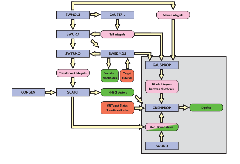
Figure 1: Schematic of the UKRmol inner region codes with the addition of CDENPROP. The shaded rectangle encloses the routines that are required to produce transition matrix elements. Red boxes indicate input from the target calculation, pink boxes input/output for inner region use, and green boxes represent input/output from/to the outer region. The $(N+1)$ Bound states box is both green and pink indicating that these states may be constructed either using outer region, or inner regions codes.

The UKRmol code suite (including CDENPROP) is a project registered on CCPForge, providing an online repository which allows for collaborative work using the Subversion version control system.

A calculation is performed in 3 stages, first the target electronic states are constructed and transition moments between them, then the inner region Hamiltonian is constructed and solved, finally the R-matrix is constructed, propagated in the outer region and matched to asymptotics. CDENPROP resides primarily in the inner region stage, fig. (1) shows a schematic of the various inner region codes with the most important inputs and outputs. The shaded rectangle indicates steps required to produce inner region dipoles, including the new module CDENPROP that implements the theory of the preceding section. CDENPROP takes as input, target states and transition dipoles from the target calculation, dipole integrals between both bound and continuum orbitals restricted to the inner region, inner regions wavefunctions (the $(N+1)$ CI vectors in fig. (1)) and, optionally, bound states produced by the outer region code BOUND. It outputs the inner region dipoles and Dyson orbitals. We note that CDENPROP is also capable of calculating transition dipoles between the target states.

CDENPROP borrows routines from the existing UKRmol code, DENPROP, for the application of Slater’s rules. Aside from the construction of the density matrix, there is another key difference between the two codes. DENPROP constructs the density matrix for each state pair, reducing the density matrix in symbolic form to a small set of orbitals pairs and corresponding coefficients, and then picks up the relevant dipole integrals, a procedure that is memory efficient but scales like $\mathcal{O}(n^{4})$ with the basis set size, $n$, this is ameliorated by the sparseness of the density matrix when each basis function is a single Slater determinant, and by the fact that, generally, during a target run, only a small subset of the target states are required. Neither of these conditions hold in the inner region, where the contracted basis leads to the $\mathrm{C-L^{2}}$ blocks being non-sparse and where dipoles between all the inner region wavefunctions may be required. The procedure DENPROP uses rapidly becomes unfeasible as the basis set size increases. The technique outlined in the previous section picks up the dipole integrals first, and then multiplies in the state coefficients, giving a scaling of $\mathcal{O}(n^{3})$ and only requiring a single pickup of the dipole integrals, but paying a penalty in increased memory requirements. We use sparse matrix routines throughout the code where appropriate. It is important to note that the memory requirements are of the same order as the Hamiltonian construction and diagonalisation code SCATCI [2] and so memory issues tend to show up, and are addressed, at this stage, prior to reaching CDENPROP.

4 Conclusions

We have described our newly developed technique for calculating the inner region transition matrix elements needed in a wide range of applications. The technique is implemented in the code module, CDENPROP, and takes advantage of the structure of the inner region basis to efficiently calculate the transition matrix elements. Finally, we note that we have successfully applied the new code in studies on angular resolved photoionization from aligned CO₂ [8, 6], He photoionization and electron-He⁺ scattering in a weak D.C. external field (Brambila et al. in prep.) and to describe the recombination step in high harmonic generation experiments (Harvey et al. in prep.). The new code also forms an integral part of the ongoing development of the molecular time-dependent R-matrix approach.

References

• [1] J.Β M. Carr, P.Β G. Galiatsatos, J.Β D. Gorfinkiel, A.Β G. Harvey, M.Β A. Lysaght, D.Β Madden, Z.Β MaΕ‘Γ­n, M.Β Plummer, J.Β Tennyson, H.Β N. Varambhia, UKRmol: a low-energy electron- and positron-molecule scattering suite, Eur. Phys. J. D 66Β (3) (2012) 1–11. doi:10.1140/epjd/e2011-20653-6.
• [2] J.Β Tennyson, A new algorithm for Hamiltonian matrix construction in electron-molecule collision calculations, J. Phys. B: At. Mol. Opt. Phys. 29Β (9) (1996) 1817. doi:10.1088/0953-4075/29/9/024.
• [3] R.Β McWeeny, B.Β T. Sutcliffe, Methods of molecular quantum mechanics, Academic Press, 1969.
• [4] J.Β Tennyson, Electron-molecule collision calculations using the R-matrix method, Physics Reports 491Β (2) (2010) 29–76. doi:10.1016/j.physrep.2010.02.001.
• [5] P.Β G. Burke, R-Matrix Theory of Atomic Collisions: Application to Atomic, Molecular and Optical Processes, Springer, 2011.
• [6] A.Β G. Harvey, D.Β S. Brambila, F.Β Morales, O.Β Smirnova, Submitted for publication.
• [7] B.Β K. Sarpal, S.Β E. Branchett, J.Β Tennyson, L.Β A. Morgan, Bound states using the R-matrix method: Rydberg states of HeH, J. Phys. B: At. Mol. Opt. Phys. 24Β (17) (1991) 3685. doi:10.1088/0953-4075/24/17/006.
• [8] A.Β Rouzee, A.Β G. Harvey, F.Β Kelkensberg, D.Β S. Brambila, W.Β K. Siu, G.Β Gademann, O.Β Smirnova, M.Β J.Β J. Vrakking, Submitted for publication.