Phase retrieval of reflection and transmission coefficients
from Kramers-Kronig relations

Abstract

Analytic and passivity properties of reflection and transmission coefficients of thin-film multilayered stacks are investigated. Using a rigorous formalism based on the inverse Helmholtz operator, properties associated to causality principle and passivity are established when both temporal frequency and spatial wavevector are continued in the complex plane. This result extends the range of situations where the Kramers-Kronig relations can be used to deduce the phase from the intensity. In particular, it is rigorously shown that Kramers-Kronig relations for reflection and transmission coefficients remain valid at a fixed angle of incidence. Possibilities to exploit the new relationships are discussed.

I Introduction

Phase data have become a key in multilayer optics since they drive resonance effects and broad-band properties in most optical coatings Macleod ; Baum ; Thelen ; Tikhon , with additional recent applications in the field of chirped mirrors Pervak . Moreover such data provide a complementary characterization tool to probe multilayers and solve inverse problems, in order to check the agreement with the expected design, etc… For these reasons a number of optical techniques were developed to investigate phase data, in addition to reflection and transmission energy coefficients. Ellipsometry has widely been used in this context, but provides differential phase data not available at normal illumination. Absolute phase data are more complex to extract and often involve interferential techniques Pervak09 ; Xue09 more sensitive to the surrounding. Within this framework complementary techniques to extract phase data at low-cost with high accuracy remains a challenge for a number of applications including optical microscopy. Among them, the Kramers-Kronig techniques deserve to be furthermore explored.

Kramers-Kronig relationships are classically based on a causality principle which describes the temporal behavior of a material submitted to excitation Jackson ; Landau8 . Such behavior can be seen as the result of a linear filter, that is, the result of a convolution product between the input excitation and another function characteristic of the material microstructure (permittivity, permeability…); this last function vanishes at negative instants, so that the material response at time $t$ depends on all excitation values at lower instants ($\text{{t}}^{\prime}<\text{{t}}$). Due to this intuitive property, mathematical transformations emphasize specific integrals in the Fourier plane that connect the real (Re$\,\varepsilon$) and imaginary (Im$\,\varepsilon$) parts of permittivity (for instance) Jackson ; Landau8 . In other words, it is well established that Im$\,\varepsilon$ at one frequency can be deduced from the values of Re$\,\varepsilon$ at all other frequencies, and conversely. This is a general result for signals so-called causal signals. Hence the amplitude reflection from a multilayer should also follow the Kramers-Kronig criterion, since the reflected field can also be written as the result of a linear filter, where the characteristic function is a double inverse Fourier transform (over temporal and spatial frequency) of the reflection coefficient. In this case the consequence is that the spectral phase of the stack can be retrieved from the intensity spectral properties of the same stack. Several authors have worked on this topic in various situations of multilayers GO91 ; TBP97 . However, as pointed out in the literature, serious difficulties remain and result from the existence of zeros in reflection spectra since they produce branch points and cuts when the complex logarithm is used Nasha95 ; Lee97 ; Andre10 to separate the phase from the modulus. In addition, to our knowledge, a rigorous proof of the possibility to use Kramers-Kronig relation at oblique incidence has not been established.

In this paper, we use the techniques derived in GT10 to show new properties of reflection and transmission coefficients of multilayered stacks. First, the usual analytic properties with respect to the complex frequency $z$, currently stated at normal incidence Tikhon93 ; TBP97 , are generalized to the complex wavevector k. This new property extends the possibility to use the analyticity for all angles of incidence from 0 to 90 degrees. Next, a second property, denominated by “passivity property”, shows that the sum of the reflection coefficient with a phase shift, $\exp[-i\beta_{\circ}(\omega,\boldsymbol{\text{{k}}})\text{{d}}]+r(\omega,\boldsymbol{\text{{k}}})$, cannot vanish in an appropriate domain of the complex frequency and wavevector. This passivity property makes it possible to apply the complex logarithm without alteration of the analytic properties with respect to the complex frequency and wavevector. They are used to propose alternative solutions to retrieve the phase of reflection and transmission coefficients. In particular, since the quantity $\{1+\exp[i\beta_{\circ}(\omega,\boldsymbol{\text{{k}}})\text{{d}}]\,r(\omega,\boldsymbol{\text{{k}}})\}$ cannot vanish, the proposed alternative solutions for the reflection coefficient do not use Blaschke factors Tikhon93 ; TBP97 .

II Background

Throughout this article an orthonormal basis is used: every vector x in $\mathbb{R}^{3}$ is described by its three components $\text{{x}}_{1}$, $\text{{x}}_{2}$ and $\text{{x}}_{3}$ (see Fig. 1). We start with the usual Helmholtz equation in non magnetic, isotropic and linear media, and in the absence of sources. The time-harmonic electric field $\text{{E}}(\text{{x}},\omega)$ is the solution of

$$\omega^{2}\mu_{\circ}\varepsilon(\text{{x}},\omega)\text{{E}}(\text{{x}},\omega)-\boldsymbol{\nabla\times}\boldsymbol{\nabla\times}\text{{E}}(\text{{x}},\omega)=0\,.$$ (1)

where $\boldsymbol{\nabla\times}$ is the curl operator, $\omega$ is the temporal pulsation resulting from the Fourier decomposition with respect to time, $\mu_{\circ}$ is the vacuum permeability, and $\varepsilon(\text{{x}},\omega)$ the frequency-dependent permittivity.

In the case of a stack of homogeneous layers invariant in $\text{{x}}_{1}$ and $\text{{x}}_{2}$ directions (see Fig. 1), a Fourier decomposition $\text{{E}}(\text{{x}},\omega)\longrightarrow\hskip 0.99585pt\widehat{\text{{E}}\hskip 0.99585pt}(\boldsymbol{\text{{k}}},\text{{x}}_{3},\omega)$ with respect to the space variables $(\text{{x}}_{1},\text{{x}}_{2})=\text{{v}}$ is performed,

$$\hskip 0.99585pt\widehat{\text{{E}}\hskip 0.99585pt}(\boldsymbol{\text{{k}}},\text{{x}}_{3},\omega)=\dfrac{1}{4\pi^{2}}\displaystyle\int_{\mathbb{R}^{2}}\exp[-i\boldsymbol{\text{{k}}}\cdot\text{{v}}]\text{{E}}(\text{{v}},\text{{x}}_{3},\omega)\,d\text{{v}}\,,$$ (2)

where $\boldsymbol{\text{{k}}}=(\text{{k}}_{1},\text{{k}}_{2})$ is the two-dimensional wave vector associated with the invariance planes of the geometry. Then, the electric field $\hskip 0.99585pt\widehat{\text{{E}}\hskip 0.99585pt}(\boldsymbol{\text{{k}}},\text{{x}}_{3},\omega)$ can be determined in all the multilayered stack and the surrounding homogeneous media using the admittance formalism Macleod or transfer matrix Macleod formalisms. In particular, the field $\hskip 0.99585pt\widehat{\text{{E}}\hskip 0.99585pt}(\boldsymbol{\text{{k}}},\text{{x}}_{3},\omega)$ is expressed in the surrounding homogeneous media in terms of the reflection and transmission coefficients $r(\boldsymbol{\text{{k}}},\omega)$ and $t(\boldsymbol{\text{{k}}},\omega)$ of the field amplitude.

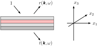
Figure 1: Reflection and transmission coefficients of a thin film multilayered stack.

In this paper, it is proposed to study the properties of the reflection and transmission coefficients with respect to both the temporal frequency and spatial wave vector extended to the complex plane: in particular, the frequency becomes the complex number $z=\omega+i\eta$, where $\eta$ is the positive imaginary part. It is stressed that these properties are closely connected, not to say equivalent, to causality principle. Indeed, from the Paley-Wiener theorem (see theorem IX.11 in RS2 ), analytic properties of a function imposes to its Fourier transform to vanish in a domain of the Fourier space. For exemple, the permittivity $\varepsilon(\text{{x}},z)$ is an analytic function in the upper half plane of complex frequencies $z=\omega+i\eta$ with positive imaginary part $\eta$. Using that $\varepsilon(\text{{x}},z)$ tends to the vacuum permittivity $\varepsilon_{\circ}$ when $|z|\rightarrow\infty$, it follows that the electric susceptibility defined by

$$\chi(\text{{x}},\text{{t}})=\int_{\mathbb{R}}\exp[-i\omega\text{{t}}]\,[\varepsilon(\text{{x}},\omega)/\varepsilon_{\circ}-1]\,d\omega\,$$ (3)

vanishes for negative values of the time variable t [here, notice that the symbol “t” is used for the time variable, while the transmission coefficient is denoted by “$t(\boldsymbol{\text{{k}}},\omega)$”]. Indeed, in that case, the integral over the frequency in the equation above, can be computed by closing the integration path by a semi circle in upper half plane which, in combination with the Cauchy’s theorem, yields $\chi(\text{{x}},\text{{t}})=0$ if $\text{{t}}<0$.

The amplitudes $r(\boldsymbol{\text{{k}}},\omega)$ and $t(\boldsymbol{\text{{k}}},\omega)$ of reflected and transmitted waves are generally used to compute the Green’s function of the multilayered stack Tom95 . Here, on the contrary, it is proposed to use the knowledge of the Green’s function to deduce the properties of the reflection and transmission coefficients. In practice, these properties will be derived from the inverse of the Helmholtz operator (1) whose the Green’s function is nothing else than the kernel. In order to address the most general properties of reflection and transmission coefficients, the Helmholtz operator is rigorously defined in the next section using the auxiliary field formalism Tip98 .

III Inverse of Helmholtz operator

We start with Maxwell’s equations. Let $\text{{E}}(\text{{x}},\text{{t}})$, $\text{{B}}(\text{{x}},\text{{t}})$ and $\text{{P}}(\text{{x}},\text{{t}})$ be respectively the time-dependent electric, magnetic and polarization fields. Then,

$$\begin{array}[]{l}\varepsilon_{\circ}\,\partial_{\text{{t}}}\text{{E}}(\text{{x}},\text{{t}})+\partial_{\text{{t}}}\text{{P}}(\text{{x}},\text{{t}})=\boldsymbol{\nabla\times}\text{{B}}(\text{{x}},\text{{t}})/\mu_{\circ}\,,\\[5.69054pt] \partial_{\text{{t}}}\text{{B}}(\text{{x}},\text{{t}})=-\boldsymbol{\nabla\times}\text{{E}}(\text{{x}},\text{{t}})\,,\end{array}$$ (4)

where $\partial_{\text{{t}}}$ is the partial derivative with respect to time. In addition to these equations, the electric field is related to the polarization through the constitutive equation

$$\text{{P}}(\text{{x}},\text{{t}})=\varepsilon_{\circ}\displaystyle\int_{-\infty}^{\text{{t}}}\chi(\text{{x}},\text{{t}}-\text{{s}})\text{{E}}(\text{{x}},\text{{s}})\,d\text{{s}}\,,$$ (5)

where $\chi(\text{{x}},\text{{t}})$ is the electric susceptibility that vanishes for negative times: $\chi(\text{{x}},\text{{t}})=0$ if $\text{{t}}<0$. According to (3), the dielectric permittivity is then defined as the Laplace transform of the susceptibility

$$\dfrac{\varepsilon(\text{{x}},z)}{\varepsilon_{\circ}}=1+\dfrac{1}{2\pi}\displaystyle\int_{0}^{\infty}\exp[iz\text{{t}}]\chi(\text{{x}},\text{{t}})\,d\text{{t}}\,.$$ (6)

Since $t$ is positive in the integral above, this permittivity is well-defined for complex frequency $z=\omega+i\eta$ with positive imaginary part Im$(z)=\eta>0$. Moreover, its derivative with respect to the complex frequency remains well defined since the function in the integral

$$\dfrac{d\varepsilon}{dz}(\text{{x}},z)=\dfrac{\varepsilon_{\circ}}{2\pi}\displaystyle\int_{0}^{\infty}(it)\exp[iz\text{{t}}]\chi(\text{{x}},\text{{t}})\,d\text{{t}}\,$$ (7)

has exponential decay for Im$(z)>0$. It follows that the permittivity $\varepsilon(\text{{x}},z)$ is an analytic function in the upper half plane of complex frequencies $z$. Finally, it is well-known that, in passive media, the electromagnetic energy must decrease with time, and thus the permittivity must have positive imaginary part Landau8 . In particular, the function

$$\sigma(\text{{x}},\omega)=\displaystyle\frac{\omega\,\text{Im}\,\varepsilon(\text{{x}},\omega)}{\pi\varepsilon_{\circ}}\geq 0\,$$ (8)

takes positive values.

In order to define rigorously the inverse of the Helmholtz operator, the auxiliary field formalism Tip97 ; Tip98 ; GT10 is used. It is based on the introduction of a new field $\text{{A}}(\text{{t}})$ denominated auxiliary field which is added to the electromagnetic field to form the total vector field $F(\text{{t}})=(\text{{E}}(\text{{t}}),\text{{B}}(\text{{t}}),\text{{A}}(t))$ [the only time-dependence of the total field $F(\text{{t}})$ appears, the other dependences are omitted]. Then, it can be shown that Maxwell’s equations can be written as the unitary time-evolution equation $\partial_{\text{{t}}}\text{{F}}(\text{{t}})=-i\mathsf{K}\text{{F}}(\text{{t}})$ where $\mathsf{K}$ is a time-independent selfadjoint operator GT10 . Next, a Laplace transform like (6) is applied to this time-evolution equation to turn to the complex frequency domain. Since the operator $\mathsf{K}$ is selfadjoint, the inverse $[z-\mathsf{K}]^{-1}$ is well-defined for all complex number $z$ with Im$(z)>0$, and is moreover an analytic function of $z$. Finally, the inverse of the Helmholtz operator is obtained by projecting the total fields $\text{{F}}(z)$ on the electric fields $\text{{E}}(z)$ in the equation involving the inverse $[z-\mathsf{K}]^{-1}$ GM12 . Let $\mathsf{P}$ be the projector defined by $\mathsf{P}\text{{F}}(z)=\text{{E}}(z)$. Then, the inverse $\mathsf{R}(z)$ of the Helmholtz operator is defined by GM12

$$\mathsf{R}(z)=\mathsf{P}\,\dfrac{1}{z-\mathsf{K}}\,\mathsf{P}\,.$$ (9)

It can be checked that, from a rigorous calculation based on the Feshbach projection formula Tip00 ; GT10 , the operator $\mathsf{R}(z)$ is precisely the inverse of the Helmholtz operator defined by equation (1). Since the projector $\mathsf{P}$ is $z$-independent, the inverse of the Helmholtz operator has the same analytic properties than the inverse $[z-\mathsf{K}]^{-1}$.

IV General properties of reflection and transmission coefficients

The most general properties of reflection and transmission coefficients are deduced from those of the inverse Helmholtz operator $\mathsf{R}(z)$ introduced in the previous section (9). Indeed, by definition, the inverse $\mathsf{R}(z)$ is related to the Green’s function $\mathsf{G}(\text{{x}},\text{{y}};z)$ by

$$[\mathsf{R}(z)f](\text{{x}})=\int_{\mathbb{R}^{3}}\mathsf{G}(\text{{x}},\text{{y}};z)f(\text{{y}})\,d\text{{y}}\,,$$ (10)

where $f(\text{{y}})$ is an “admissible” function. For example, functions $f(\text{{y}})$ and $h(\text{{x}})$ can be chosen arbitrary close to Dirac “functions” $\delta(\text{{y}}-\text{{y}}_{0})$ and $\delta(\text{{x}}-\text{{x}}_{0})$ centered at $\text{{y}}_{0}$ and $\text{{x}}_{0}$: it implies that

$$\begin{array}[]{ll}\displaystyle\int_{\mathbb{R}^{3}}\overline{h(\text{{x}})}\,[\mathsf{R}(z)f](\text{{x}})\,d\text{{x}}&=\displaystyle\int_{\mathbb{R}^{3}}\delta(\text{{x}}-\text{{x}}_{0})\left[\displaystyle\int_{\mathbb{R}^{3}}\mathsf{G}(\text{{x}},\text{{y}};z)\,\delta(\text{{y}}-\text{{y}}_{0})\,d\text{{y}}\right]\,d\text{{x}}\,=\displaystyle\int_{\mathbb{R}^{3}}\delta(\text{{x}}-\text{{x}}_{0})\,\mathsf{G}(\text{{x}},\text{{y}}_{0};z)\,d\text{{x}}\\[11.38109pt] &=\mathsf{G}(\text{{x}}_{0},\text{{y}}_{0};z)\,,\end{array}$$ (11)

which shows that properties of the inverse $\mathsf{R}(z)$ are directly transposable to the Green’s function $\mathsf{G}(\text{{x}}_{0},\text{{y}}_{0};z)$. In the particular case of multilayered stacks, the Fourier decomposition (2) is applied. The partial derivatives $\partial/\partial\text{{x}}_{1}$ and $\partial/\partial\text{{x}}_{2}$ in Maxwell’s equations are replaced by $-i\text{{k}}_{1}$ and $-i\text{{k}}_{2}$, and the Fourier transformed $\mathsf{G}(\text{{x}}_{0},\text{{y}}_{0};z)$ is denoted by $\widehat{\mathsf{G}}(\boldsymbol{\text{{k}}},\text{{x}}_{0},\text{{y}}_{0};z)$, where $\text{{x}}_{0}$ and $\text{{y}}_{0}$ are the $\text{{x}}_{3}$-component of the vectors $\text{{x}}_{0}$ and $\text{{y}}_{0}$. From the expression of the Green’s function of multilayers Tom95 , and choosing $\text{{x}}_{0}$ and $\text{{y}}_{0}$ at the top ($\text{{x}}_{3}=\text{{x}}_{u}$) or bottom ($\text{{x}}_{3}=\text{{x}}_{d}$) interfaces delimiting the multilayer, it can be deduced that

$$\begin{array}[]{ll}\widehat{\mathsf{G}}(\boldsymbol{\text{{k}}},\text{{x}}_{u},\text{{x}}_{u};z)\!\!&=-\,\dfrac{z}{2i\beta_{\circ}(\boldsymbol{\text{{k}}},z)}\,[1+r(\boldsymbol{\text{{k}}},z)]\,,\\[11.38109pt] \widehat{\mathsf{G}}(\boldsymbol{\text{{k}}},\text{{x}}_{u},\text{{x}}_{d};z)\!\!&=-\,\dfrac{z}{2i\beta_{\circ}(\boldsymbol{\text{{k}}},z)}\,t(\boldsymbol{\text{{k}}},z)\,,\end{array}$$ (12)

where $\beta_{\circ}(\boldsymbol{\text{{k}}},z)$ is uniquely defined as the square root $\beta_{\circ}(\boldsymbol{\text{{k}}},z)=\sqrt{z^{2}\varepsilon_{\circ}\mu_{\circ}-\boldsymbol{\text{{k}}}^{2}}$ with positive imaginary part. Note that $\beta_{\circ}(\boldsymbol{\text{{k}}},z)$ is also analytic for $z$ with positive imaginary part.

We are now ready to derive the general properties of the reflection and transmission coefficients. The analytic properties are deduced directly from relations (12) and (11). The analytic property of inverse Helmholtz operator $\mathsf{R}(z)$ implies the well-know result GO91 ; TBP97 stating that the coefficients $r(\boldsymbol{\text{{k}}},z)$ and $t(\boldsymbol{\text{{k}}},z)$ are analytic functions in the half plane of complex frequencies $z$ with positive imaginary part. We propose herein to extend this property to the complex wave vector k associated with the two-dimensionnal invariance of the system. After the Fourier decomposition (2), the partial derivatives $\partial/\partial\text{{x}}_{1}$ and $\partial/\partial\text{{x}}_{2}$ in Maxwell’s equations are replaced by $-i\text{{k}}_{1}$ and $-i\text{{k}}_{2}$. The resulting Fourier transformed operator $\widehat{\mathsf{K}}(\boldsymbol{\text{{k}}})$ is selfadjoint for real $\text{{k}}_{1}$ and $\text{{k}}_{2}$. Its definition can be extended to complex k (i.e. the components $\kappa_{1}$ and $\kappa_{2}$ are complex numbers) and, in that case, $\widehat{\mathsf{K}}(\boldsymbol{\text{{k}}})$ is no more selfadjoint. Then, it can be shown that the imaginary part of the operator $[z-\widehat{\mathsf{K}}(\boldsymbol{\text{{k}}})]$ defined as

$$\text{Im}[z-\widehat{\mathsf{K}}(\boldsymbol{\text{{k}}})]=\dfrac{1}{2i}\Big{\{}[z-\widehat{\mathsf{K}}(\boldsymbol{\text{{k}}})]-[z-\widehat{\mathsf{K}}(\boldsymbol{\text{{k}}})]^{\dagger}\Big{\}}\,,$$ (13)

only depends on the imaginary parts of $z$ and k. Simple calculations show that this imaginary part above is semi-bounded:

$$\text{Im}[z-\widehat{\mathsf{K}}(\boldsymbol{\text{{k}}})]\geq\text{Im}(z)-c\,|\text{Im}(\boldsymbol{\text{{k}}})|\,,$$ (14)

where $|\text{Im}(\boldsymbol{\text{{k}}})|=\sqrt{\text{Im}(\text{{k}}_{1})^{2}+\text{Im}(\text{{k}}_{2})^{2}}$ and $c=1/\sqrt{\varepsilon_{\circ}\mu_{\circ}}$. It follows that this imaginary part remains strictely positive if $\text{Im}(z)>c\,|\text{Im}(\boldsymbol{\text{{k}}})|$. Under this condition, the corresponding inverse $[z-\widehat{\mathsf{K}}(\boldsymbol{\text{{k}}})]^{-1}$ is analytic with respect to all the complex variables $z$ and k, which yields the following result.

Result 1. The reflection and transmission coefficients, $r(\boldsymbol{\text{{k}}},z)$ and $t(\boldsymbol{\text{{k}}},z)$, are analytic functions of the complex variables $z$ and $(\text{{k}}_{1},\text{{k}}_{2})=\boldsymbol{\text{{k}}}$ in the domain defined by $\text{Im}(z)>c\,|\text{Im}(\boldsymbol{\text{{k}}})|$.

Next, a new property is derived from an analogy with the passivity requirement for the electric permittivity. It is well-known that the passivity requires for the function $\varepsilon(\text{{x}},z)$ to have its imaginary part to be positive, see equation (8). Using a generalization GT10 of the Kramers and Kronig relations, it can be shown that

$$\text{Im}\{z\varepsilon(\text{{x}},z)\}\geq\text{Im}\{z\varepsilon_{\circ}\}>0\,.$$ (15)

A similar relationship can be established for the inverse of the Helmholtz operator from

$$\begin{array}[]{ll}-\text{Im}\dfrac{1}{z-\mathsf{K}}&=\dfrac{1}{2i}\left[\dfrac{1}{\overline{z}-\mathsf{K}}-\dfrac{1}{{z}-\mathsf{K}}\right]\\[11.38109pt] &=\dfrac{1}{z-\mathsf{K}}\,\text{Im}(z)\,\dfrac{1}{\overline{z}-\mathsf{K}}>0\,.\end{array}$$ (16)

Again, this expression can be extended to complex values of the wave vector k. According to the relation (14), if $\text{Im}(z)>c\,|\text{Im}(\boldsymbol{\text{{k}}})|$, then the inverse $[z-\widehat{\mathsf{K}}(\boldsymbol{\text{{k}}})]^{-1}$ is well defined and has positive imaginary part since

$$\begin{array}[]{l}-\text{Im}\dfrac{1}{z-\widehat{\mathsf{K}}(\boldsymbol{\text{{k}}})}\geq\\[11.38109pt] \quad\quad\dfrac{1}{z-\widehat{\mathsf{K}}(\boldsymbol{\text{{k}}})}\,\big{[}\text{Im}(z)-c\,|\text{Im}(\boldsymbol{\text{{k}}})|\,\big{]}\,\dfrac{1}{\overline{z}-\widehat{\mathsf{K}}(\overline{\boldsymbol{\text{{k}}}})}>0\,.\end{array}$$ (17)

It has to be noticed that, in the case of this “passivity” property, the extension to complex wave vector k is of vital importance for the transposition to the coefficients $r(\boldsymbol{\text{{k}}},z)$ and $t(\boldsymbol{\text{{k}}},z)$ at non normal incidence $\boldsymbol{\text{{k}}}\neq\boldsymbol{0}$. Indeed, for all propagative waves it is possible to choose $\boldsymbol{\text{{k}}}=z\text{{u}}$ with $\text{{u}}^{2}<\sqrt{\varepsilon_{\circ}\mu_{\circ}}$, so that the relation $\text{Im}(z)>c\,|\text{Im}(\boldsymbol{\text{{k}}})|$ remains true. Hence, the square root $\beta_{\circ}(\boldsymbol{\text{{k}}},z)$ in equation (12) can be written $\beta_{\circ}(\boldsymbol{\text{{k}}},z)=z\sqrt{\varepsilon_{\circ}\mu_{\circ}-\text{{u}}^{2}}$, and the following result can deduced from (17) and the first line of (12).

Result 2. The reflection coefficient $r(\boldsymbol{\text{{k}}},z)$ must satisfy

$$\text{Re}\{1+r(z\text{{u}},z)\}>0\,,$$ (18)

where u is defined by $\boldsymbol{\text{{k}}}=z\text{{u}}$ and has modulus square $\text{{u}}^{2}<\varepsilon_{\circ}\mu_{\circ}$.

In practice, the function $\{1+r(z\text{{u}},z)\}$ has positive real part for all complex frequency $z$ with positive imaginary part, and for all fixed angle $\theta$ from normal incidence defined by $\text{{u}}^{2}=\varepsilon_{\circ}\mu_{\circ}\sin^{2}\theta$. Thus the result (18) can be applied to only propagating waves. For evanescent waves, if the wave vector is written $\boldsymbol{\text{{k}}}=z\text{{u}}$ with $\text{{u}}^{2}>\varepsilon_{\circ}\mu_{\circ}$, both relations (16) and (17) need not to be correct, and then there is no simple condition for the reflection coefficient.

Finally, an addionnal result can be obtained evaluating the Green’s function at a distance $\text{{d}}/2$ above the top interface delimiting the multilayered stack: $\text{{x}}_{0}=\text{{y}}_{0}=\text{{x}}_{u}+\text{{d}}/2$. This distance introduces the phase shift $\exp[i\beta_{\circ}(\boldsymbol{\text{{k}}},z)\text{{d}}]$ and the first line of (12):

$$\begin{array}[]{l}\widehat{\mathsf{G}}(\boldsymbol{\text{{k}}},\text{{x}}_{u}+\text{{d}}{\color[rgb]{0,0,0}{/2}},\text{{x}}_{u}+\text{{d}}{\color[rgb]{0,0,0}{/2}};z)=\\[5.69054pt] \quad\quad-\,\dfrac{z}{2i\beta_{\circ}(\boldsymbol{\text{{k}}},z)}\{1+\exp[i\beta_{\circ}(\boldsymbol{\text{{k}}},z)\text{{d}}]r(\boldsymbol{\text{{k}}},z)\}\,.\end{array}$$ (19)

Thus the result 2 can be generalized as follows.

Result 3. The reflection coefficient $r(\boldsymbol{\text{{k}}},z)$ must satisfy

$$\text{Re}\{1+\exp[i\beta_{\circ}(\boldsymbol{\text{{k}}},z)\text{{d}}]r(\boldsymbol{\text{{k}}},z)\}>0\,,$$ (20)

for all complex variables $z$ and $(\text{{k}}_{1},\text{{k}}_{2})=\boldsymbol{\text{{k}}}$ in the domain defined by $\text{Im}(z)>c\,|\text{Im}(\boldsymbol{\text{{k}}})|$.

It is stressed that the results 2 and 3 extend the well known relation TBP97 derived from the calculation of the Poynting vector flux for real frequency and wavevector. Indeed, let $z=\omega$ be purely real, then $\exp[i\beta_{\circ}(\boldsymbol{\text{{k}}},z)\text{{d}}]$ becomes a pure phase shift with unit modulus. let $d$ vary, then relation (20) shows that $r(\boldsymbol{\text{{k}}},z)$ is located on a circle with radius below unity, i.e. $|r(\boldsymbol{\text{{k}}},\omega)|\leq 1$.

V Phase retrieval

V.1 Kramers-Kronig relations at a fixed oblique incidence

In this section, the Kramers-Kronig relations are used to retrieve the phase of reflection and transmission coefficients from their modulus (intensity of the field). Let $f(z)$ be an analytic function in the half plane of complex numbers $z$ with positive imaginary part, which vanishes at the infinity: $f(z)\longrightarrow 0$ for $|z|\longrightarrow\infty$. Then Kramers and Kronig relations leads to

$$\text{Im}\{f(\omega)\}=\dfrac{1}{\pi}\mathcal{P}\displaystyle\int_{\mathbb{R}}\dfrac{\text{Re}\{f(\nu)\}}{\omega-\nu}\,d\nu\,,$$ (21)

where the symbol $\mathcal{P}$ means that the Cauchy principal value of the integral. In order to separate the phase from the modulus of a function, it is convenient to apply the complex logarithm $\ln$. It is important to note that, the complex logarithm must be applied to a non vanishing function to preserve the analytic properties. This condition will be ensured by the results 2 and 3 for the function containing the reflection coefficient. As to the transmission coefficient, the well know result on the Poynting vector flux can be used: for Im$z>0$

$$1-|r(\boldsymbol{\text{{k}}},z)|^{2}-|t(\boldsymbol{\text{{k}}},z)|^{2}>0\,.$$ (22)

It implies that the modulus of the transmission and reflection coefficients is strictly smaller than unity. In particular, The transmission coefficient $t(\boldsymbol{\text{{k}}},z)$ must satisfy

$$|\exp[i\beta_{\circ}(\boldsymbol{\text{{k}}},z)\text{{d}}]t(\boldsymbol{\text{{k}}},z)|<1\,,$$ (23)

for all complex variables $z$ and $(\text{{k}}_{1},\text{{k}}_{2})=\boldsymbol{\text{{k}}}$ in the domain defined by $\text{Im}(z)>c\,|\text{Im}(\boldsymbol{\text{{k}}})|$. Also, is well known that the transmission coefficient cannot vanish TBP97 [$t(\boldsymbol{\text{{k}}},\omega)=0$ implies that the field must vanish in all the space, which is impossible when the multilayered stack is illuminated by a plane wave]. Finally, it is stressed that the extension of analytic properties to complex wave vector, stated in result 1, is crucial to keep fixed the angle of incidence for all (complex) frequencies. Thus, for $\boldsymbol{\text{{k}}}=z\text{{u}}$, the Kramers and Kronig relations (21) can be applied to functions

$$\begin{array}[]{l}f_{t}(z)=\ln\{t(z\text{{u}},z)\}\,,\\[5.69054pt] f_{r}(z)=\ln\{{\color[rgb]{0,0,0}{1+\exp[i\beta_{\circ}(z\text{{u}},z)\text{{d}}]r(z\text{{u}},z)}}\}\,.\end{array}$$ (24)

Thus we can propose solution to determine the phase of the transmission and reflection coefficients using the relations

$$\begin{array}[]{l}\text{Phase}\{t(\omega\text{{u}},\omega)\}=\dfrac{1}{2\pi}\mathcal{P}\!\!\displaystyle\int_{\mathbb{R}}\dfrac{\ln|t(\nu\text{{u}},\nu)|^{2}}{\omega-\nu}\,d\nu\,,\\[11.38109pt] \text{Phase}\{{\color[rgb]{0,0,0}{1+\exp[i\beta_{\circ}(\omega\text{{u}},\omega)\text{{d}}]r(\omega\text{{u}},\omega)}}\}=\\[5.69054pt] \quad\quad\dfrac{1}{2\pi}\mathcal{P}\!\!\displaystyle\int_{\mathbb{R}}\dfrac{\ln|{\color[rgb]{0,0,0}{1+\exp[i\beta_{\circ}(\nu\text{{u}},\nu)\text{{d}}]r(\nu\text{{u}},\nu)}}|^{2}}{\omega-\nu}\,d\nu\,.\end{array}$$ (25)

As a final step, the modulus and the phase of the reflection coefficient $r(\omega\text{{u}},\omega)$ is directly deduced from the knowledge of both the modulus and the phase of $\{\,{\color[rgb]{0,0,0}{1+\exp[i\beta_{\circ}(\omega\text{{u}},\omega)\text{{d}}]r(\omega\text{{u}},\omega)}}\}$.

It is stressed that our result, with the wavevector $\boldsymbol{\text{{k}}}=z\text{{u}}$ related to the frequency $z$ to keep constant incidence angle, is more general than one with the wavevector k set to a real constant. Indeed, in the case where k is constant, there is no need to extend the properties stated for the frequency to complex wavevector. Also, with k constant, the Kramers-Kronig relations are difficult to exploit since the incident angle varies according to the frequency, and especially both regimes of propagating and evanescent waves are addressed when the frequency describe the whole spectrum.

In practice, the intensity is obtained in a finite interval of frequencies while the use of Kramers-Kronig relations requires measurements over all the frequency spectrum. This difficulty, which is not considered in this paper, can be overcome by a normalization procedure as proposed in GO91 .

In the next subsection, solutions are discussed to measure the modulus (intensity) of the functions $|t(\omega\text{{u}},\omega)|^{2}$ and $|{\color[rgb]{0,0,0}{1+\exp[i\beta_{\circ}(\omega\text{{u}},\omega)\text{{d}}]r(\omega\text{{u}},\omega)}}|^{2}$ from which the phase of reflection and transmission coefficients can be deduced.

V.2 Discussion

First, it is stressed that our results provide a rigorous proof showing that the techniques already established GO91 to retrieve the phase from the intensity can be used in non-normal incidence. For instance formula (25) can be used directly for the transmission coefficient to retrieve the phase of the transmission coefficient from the measurement of the transmitted intensity.

As to the reflection coefficient, formula (25) invites us to consider the quantity $|1+r(\boldsymbol{\text{{k}}},\omega)|^{2}$ which is the field intensity at the top interface delimiting the multilayered stack. This quantity can be determined by measuring several physical quantities. For instance, the fluorescence of excited atoms (or molecules) located at the top interface can be directly related to the the desired field intensity using the fluctuation-dissipation theorem Rytov89 ; Joulain09 . To obtain this effect, it is necessary to add at the top interface of the multilayer a very thin absorbing layer in which the emitters are implanted. Note that the additional layer has to be sufficiently thin to avoid the significant perturbation of the reflectivity properties. Also, if some roughtness is added to the top interface, then the scattered intensity is proportionnal to the field intensity. In such case, the knowledge of the factor of proportionality requires a precise knowledge of the structure. It is stressed that this can be probably more simple to obtain such factor than the whole set of complex zeros of the reflection coefficient and the associated Blaschke factors. Finally, it has to be noticed that the reflected field can be superimposed to the incident field in order to obtain directly the quantity $|{\color[rgb]{0,0,0}{1+\exp[i\beta_{\circ}(\omega\text{{u}},\omega)\text{{d}}]\,r(\omega\text{{u}},\omega)}}|^{2}$ (see figure 2, lower panel). Here, the convenience to use a setup like the one shown on figure (2) to obtain $|{\color[rgb]{0,0,0}{1+\exp[-i\beta_{\circ}(\omega\text{{u}},\omega)\text{{d}}]\,r(\omega\text{{u}},\omega)}}|^{2}$ has to be compared with the direct measurement of the phase, in order to estimate the relevance of such a proposition.

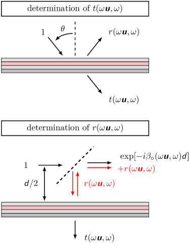
Figure 2: Top panel: Direct determination of the transmitted intensity $|t(\omega\text{{u}},\omega)|^{2}$. Lower panel: Determination of the quantity $|{\color[rgb]{0,0,0}{1+\exp[i\beta_{\circ}(\omega\text{{u}},\omega)\text{{d}}]\,r(\omega\text{{u}},\omega)}}|^{2}$ from which the phase of the reflection coefficient $r(\omega\text{{u}},\omega)$ can be deduced.

VI Conclusion

We went further in the investigation of causality principles in the sense that some multilayer responses were shown to be analytic when both Fourier variables ($\omega$ and k) are extended to the domain of the complex plane defined by Im$(z)>c|$Im$(\boldsymbol{\text{{k}}})|$. This result allowed us to extend the Kramers-Kronig relationships to the more general situation of oblique incidence. These relations can be applied to the complex logarithm of the energy transmission function, but also to the quantity $\ln|{\color[rgb]{0,0,0}{1+\exp[i\beta_{\circ}(\omega\text{{u}},\omega)\text{{d}}]\,r(\omega\text{{u}},\omega)}}|^{2}$, thus providing a new way to investigate phase. From the point of view of experiment, this last quantity can be approach with luminescence, scattering measurements, or using an interferometer.

References

- (1) H. A. Macleod, Thin-Film Optical Filters (Taylor & Francis, 2001), third edn.
- (2) P. W. Baumeister, Optical Coating Technology (SPIE Press Book, 2004).
- (3) A. Thelen, Design of Optical Interference Coatings (McGRAW-HILL Book Company, 1989).
- (4) S. A. Furman and A. V. Tikhonrarov, Basics of Optics of Multilayer Systems (Editions Frontieres, 1992).
- (5) V. Pervak, C. Teisset, A. Sugita, S. Naumov, F. Krausz, and A. Apolonski, “High-dispersive mirrors for femtosecond lasers,” Optics Express 16, 10 220 (2008).
- (6) T. V. Amotchkina, A. V. Tikhonravov, M. K. Trubetskov, D. Grupe, A. Apolonski, and V. Pervak, “Measurement of group delay of dispersive mirrors with white-light interferometer,” Appl. Opt. 48, 949 (2009).
- (7) H. Xue, W. Shen, P. L. Gu, Y. Z. Zhang, and X. Liu, “Measurement of absolute phase shift on reflection of thin films using white-light spectral interferometry,” Chinese Optics Letters 7, 446 (2009).
- (8) J. D. Jackson, Classical Electrodynamics (Whiley, New York, 1998), third edn.
- (9) L. D. Landau, E. M. Lifshitz, and L. P. Pitaevski, Electrodynamics of Continuous Media (Courses of Theoretical Physics; V. 8) (Robert Maxwell, M. C., 1984), second edn., iSBN 0-08-030275-0.
- (10) P. Grosse and V. Offermann, “Analysis of reflectance data using the Kramers–Kronig relation,” Appl. Phys. A 52, 138 (1991).
- (11) A. V. Tikhonravov, P. W. Baumeister, and K. V. Popov, “Phase properties of multilayers,” Applied Optics 36, 4382 (1997).
- (12) P. L. Nasha, R. J. Bella, and R. Alexanderb, “On the Kramers-Kronig relation for the phase spectrum,” J. Modern Opt. 42, 1837 (1995).
- (13) M. H. Lee and O. I. Sindoni, “Kramers-Kronig relations with logarithmic kernel and application to the phase spectrum in the Drude model,” Phys. Rev. E 56, 3891 (1997).
- (14) J.-M. André, K. L. Guen, M. Jonnard, J. Mahne, A. Giglia, and S. Nannarone, “On the Kramers–Kronig transform with logarithmic kernel for the reflection phase in the Drude model,” J. Modern Opt. 57, 1504 (2010).
- (15) B. Gralak and A. Tip, “Macroscopic Maxwell’s equations and negative index materials,” J. Math. Phys 51, 052 902 (2010).
- (16) A. V. Tikhonravov, “Some theoretical aspects of thin-film optics and their applications,” Applied Optics 32, 5417 (1993).
- (17) M. Reed and B. Simon, Fourier analysis, self-adjointness, Vol. (Methods of modern mathematical physics; V. 2) (Academic Press, 1975).
- (18) M. S. Tomaś, “Green function for multilayers: Light scattering in planar cavities,” Phys. Rev. A 51, 2545 (1995).
- (19) A. Tip, “Linear absorptive dielectric,” Phys. Rev. A 57, 4818–4841 (1998).
- (20) A. Tip, “Canonical formalism and quantization for a class of classical fields with application toradiative atomic decay in dielectric,” Phys. Rev. A 56, 5022–5041 (1997).
- (21) B. Gralak and D. Maystre, “Negative index materials and time-harmonic electromagnetic field,” C. R. Physique 13, 786 (2012).
- (22) A. Tip, A. Moroz, and J.-M. Combes, “Band structure of absorptive photonic crystals,” J. Phys. A: Math. Gen. 33, 6223 (2000).
- (23) S. M. Rytov, Y. A. Kravtsov, and V. I. Tatarskii, Principles of Statistical Radiophysics 3: Elements of Random Fields (Springer, Berlin, 2009).
- (24) P. Ben-Abdallah, K. Joulain, J. Drevillon, and G. Domingues, “Tailoring the local density of states of nonradiative field at the surface of nanolayered materials,” Appl. Phys. Lett. 94, 153 117 (2009).