Properties of phoneme $N$-grams across the world’s language families

Abstract

In this article, we investigate the properties of phoneme $N$-grams across half of the world’s languages. We investigate if the sizes of three different $N$-gram distributions of the world’s language families obey a power law. Further, the $N$-gram distributions of language families parallel the sizes of the families, which seem to obey a power law distribution. The correlation between $N$-gram distributions and language family sizes improves with increasing values of $N$. We applied statistical tests, originally given by physicists, to test the hypothesis of power law fit to twelve different datasets. The study also raises some new questions about the use of $N$-gram distributions in linguistic research, which we answer by running a statistical test.

  Keywords: N-grams, ASJP, language families. 

1   Introduction and related work

1.1 Power laws

Many real-life phenomena such as word-type frequencies in a corpus, degrees of nodes in a network representation of the internet, the number of species in a genus of mammals and populations of cities follow a power law distribution. Power law distributions seem ubiquitous in nature and many other phenomena are also claimed to obey a power law Clauset et al., (2009). Computational linguists will typically have come across power laws in a form popularly known as Zipf’s law Zipf, (1935). Zipf’s law is stated as $f\propto r^{-1}$, where $f$ and $r$ is the frequency and rank of a word type $x$. This is a special case of the power law with the probability density function $p(x)$ defined as $p(x)=Cx^{-\alpha}$ where $\alpha=1$. is the scaling parameter ($\alpha>1$) and $C$ is the normalizing constant. If $p(x)$ is lower-bounded at $x_{min}$ then the power law assumes the form of $p(x)=(\alpha-1)x_{min}^{\alpha-1}\cdot x^{-\alpha}$. Power law is just one member of a larger class of distributions called large number of rare events (LNRE) distributions Baayen, (1991). As pointed by Evert and Baroni, (2007), LNRE distributions have applications in NLP/CL. LNRE distributions can be used to predict the total vocabulary size from a smaller sample. We now turn to a discussion of some recent work in computational historical linguistics where power laws play a central role in the argumentation.

There are about $7000$ languages in the world Lewis, (2009); Hammarström, (2010), forming more than $120$ families according to the Ethnologue, whereas more than $400$ are listed by Hammarström, (2010). A language family is a group of related languages (or a single language when there are no known related languages, such as Basque) descended from a common ancestor Campbell and Poser, (2008). Each of these language families is assigned a tree structure in at least two classifications Lewis, (2009); Hammarström, (2010). The size of a language family is defined as the number of related languages included in the family. Wichmann, (2005) observes that the frequency-rank plot of the sizes of language families (as defined in Ethnologue) seems to follow a power law. Figure 1(a) (reproduced from Wichmann, 2005) is plotted on a log-log scale and shows a slight deviation from the regression line in the region of $50$ and $\geq 100$. Figure 1(b) shows the frequency-rank plot for Hammarström,’s classification.

There is a slight deviation from the strict adherence to the straight line in Figure 1(b). However, the goodness-of-fit $r^{2}$ is in the range of $0.957$ and $0.98$ in both the classifications. Looking into the closely related field of linguistic typology, Maslova, (2008) proposes that meta-typological distributions obey power law. A meta-typological distribution is defined as the number of languages having a particular linguistic feature value, such as a particular word order or a phoneme inventory of a particular size (e.g., small, medium, or large). In response, Cysouw, (2010) proposes that the distribution is actually exponential masquerading as a power law.

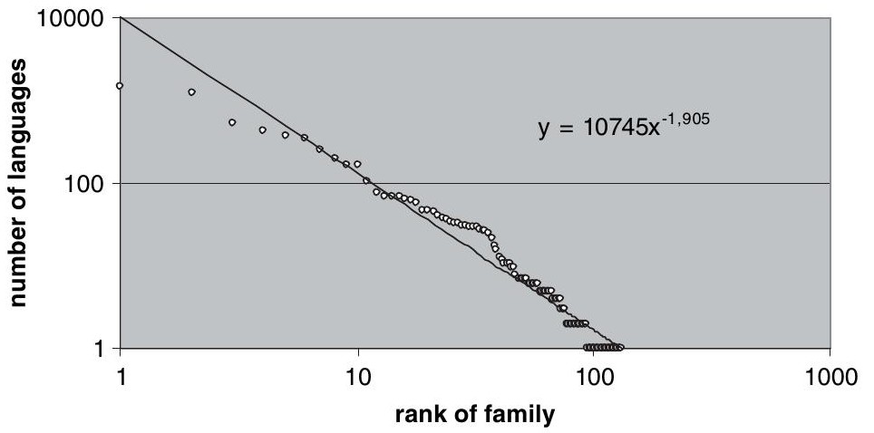
(a) Wichmann, (2005).

(b) Hammarström, (2010).

Figure 1: Frequency-rank plots for two different classifications along with the $r^{2}$ and the regression-lines generated using a commonly available spreadsheet package.

1.2 Testing power laws

The scaling parameter _sp, – estimated using a spreadsheet package – in Figures 1(a) and 1(b) is $1.905$ and $1.36$ respectively. Apart from the high $r^{2}$ value, there seems to be no independent statistical test for the support of a power law. However, a recent paper by Clauset et al., (2009) revisited this topic and proposed a number of statistical tests for validating power law models. The authors provide a maximum likelihood estimate of the two parameters, $x_{min}$ and and a method for computing the statistical significance score of the estimates. Further, they test the superiority of the power law with respect to candidate distributions, listed in Table 1.

In a recent paper, Jäger, (2012) applied the statistical tests of Clauset et al., (2009) to test the fit of the power law model to global linguistic datasets such as frequency of color terms, phonological templates for selected basic vocabulary items, and meta-typological distributions. Jäger, also applied a series of statistical tests to Maslova,’s data and showed that a power law with exponential cutoff describes the data better than a power-law model.

name	probability density function $p(x)$	# of parameters ($m$)
power law (PL)	$(\alpha-1)x_{min}^{\alpha-1}x^{-\alpha}$	$1$
power law with exponential cutoff (PLWC)	$\frac{{}^{1-\alpha}}{\Gamma(1-\alpha,\lambda x_{min})}x^{-\alpha}e^{-\lambda x}$	$2$
log-normal (LN)	$\sqrt{\frac{2}{\pi{}^{2}}}\left[\operatorname{erfc}\left(\frac{\ln x_{min}-\mu}{\sqrt{2}\sigma}\right)\right]^{-1}\frac{1}{x}\exp\left[{-\frac{(\ln x-\mu)^{2}}{2{}^{2}}}\right]$	$2$
exponential ($\exp$)	$\lambda e^{\lambda x_{min}}e^{-\lambda x}$	$1$
stretched exponential (str $\exp$)	$\beta\lambda e^{\lambda x_{min}}x^{\beta-1}e^{-\lambda x}$	$2$
gamma ()	$\frac{1}{\Gamma(k){}^{k}}x^{k-1}e^{-x/\theta}$	$2$

Table 1: List of various candidate distributions and the number of parameters in each model. These distributions are popularly referred to as “heavy-tail” distributions.

The standard method for testing a power law hypothesis consists of plotting a frequency-rank plot on a log-log scale and applying a linear regression. The linear regression boils down to determining the parameters of $\log p(x)=c+\alpha\log(x)$. However, Clauset et al., (2009) warn against this. Further, they demonstrate that the value of estimated differs largely from that derived from the regression analysis. The validity of the power law is tested through the following steps:

• Estimate _sp and $r^{2}$ using a spreadsheet package by plotting the frequency-rank plot of the data on a log-log scale.

• Estimate _est and $x_{min}$ based on the maximum likelihood criterion ($L$).

• The preference of a power law to rest of the candidate distributions is tested through a likelihood ratio test Dunning, (1993) under a significance criterion of $p\leq 0.1$.

• The absolute goodness-of-fit of a model is computed using the Akaike Information criterion which is defined as in 1, $m$ is the number of parameters and $L$ is the goodness-of-fit. The model with lowest AIC is the best fit.

  $$AIC=2m-2\log(L)$$ (1)

Jäger, simplifies the computation of for discrete data by assuming a continuous approximation of the power-law model and fixing $x_{min}$ at $0.5$. This assumption implies that all data points in a dataset completely fit a power-law model. However, it can always be the case that only a part of the dataset follows a power-law model. As a necessary diversion, it is useful to know the computation of $x_{min}$. The scaling parameter is estimated by successive removal of the lowest value of $x$. The fitted distribution is then compared to the empirical distribution through a Kolmogorov-Smirnov statistic ($D$). The value of $x$ which minimizes $D$ is chosen as $x_{min}$.

In this paper, we find that the rank plot of the size of phoneme $N$-grams for 45 language families seems to obey a power law distribution as given in Figure 2(a). This finding is in parallel to that of Wichmann, (2005). By applying the statistical procedure mentioned above, we attempt to establish whether the family sizes given in three different language classifications actually obey a power law. Subsequently we test if the phoneme $N$-grams also obey a power law model. We describe the database in the next section.

2   Database

In this section, we describe the global linguistic database (depicted in Figure 2(a)). A consortium of international scholars known as ASJP (Automated Similarity Judgment Program; Wichmann et al., 2011) have collected reduced word lists – $40$ items from the original $200$ item Swadesh word lists Swadesh, (1955), selected for maximal diachronic stability – for more than half of the world’s languages and embarked on an ambitious program for investigating automated classification of the world’s languages. The ASJP database in many cases includes more than one word list for different varieties of a language (identified through its ISO 693-3 code). A word list is included into the database if it has attestations of at least $28$ of the $40$ items ($70\%$).

Only language families with at least $4$ members are included in our experiments. This leaves a dataset with $45$ language families representing $3151$ languages (or $4524$ word lists) of the world. The names of the language families are as defined in the Ethnologue. A word list might include known borrowings marked as such and these are not used in our experiments. The words in the ASJP database are transcribed using a reduced phonetic transcription known as ASJP code consisting of $34$ consonants, $7$ vowels and a symbol for nasalization, and two other ‘modifiers’, which are used to indicate that preceding symbols combine as single segments. All click sounds are reduced to a single click symbol and distinctions such as tones, vowel length, and stress are ignored. The computation of a phoneme $N$-gram profile for a language family is described in section 3. The frequency-rank plot of the language families in the current sample is shown in Figure 2(b). The regression shows a $r^{2}$ value of $0.85$ which is quite high.

(a) World map

(b) Frequency-rank plots

Figure 2: ASJP word lists on world map and the plots with $r^{2}$ values for families from Ethnologue.

3   Experiments and results

All the word lists belonging to a single language family are merged together. Recall that the ASJP database can include more than one word list – representing different varieties – for a language. All the consecutive symbol sequences of length varying from $1$–$5$ are extracted and the size of the $N$-gram profile is defined as the total number of unique $1$–$N$-grams obtained through this procedure. Thus, a $3$-gram profile consists of all the phoneme $1$-, $2$- and $3$-grams. The size of the $3$-, $4$- and $5$-gram profiles for each of the language families as defined in the Ethnologue is given in Table 2. In effect, an $N$-gram profile is the sum of all the $n$-gram types leading up to $N$. As evident from right panel of Figure 3, each of the $N$-gram profiles, $N\geq 3$, seem to follow a power law.

When a power law regression is applied to each of the frequency-rank plots, the goodness-of-fit $r^{2}$ is $0.91$, $0.96$ and $0.97$ for $3$-grams, $4$-grams and $5$-grams respectively. The $r^{2}$ value of both $1$-grams and $2$-grams is quite low, only $0.49$ and $0.73$ when compared to the $r^{2}$ value of the number of languages, $0.85$. We also plot the frequency-rank plots for each $n$-gram type in the left panel of Figure 3. The $r^{2}$ values are quite high and are $0.84$, $0.93$ and $0.94$ respectively. The $r^{2}$ scores in Figure 1(a) for $4$–$5$ grams are very high and fall within the range of the correlation of $0.957$ (with language family size), reported by Wichmann, 2005.

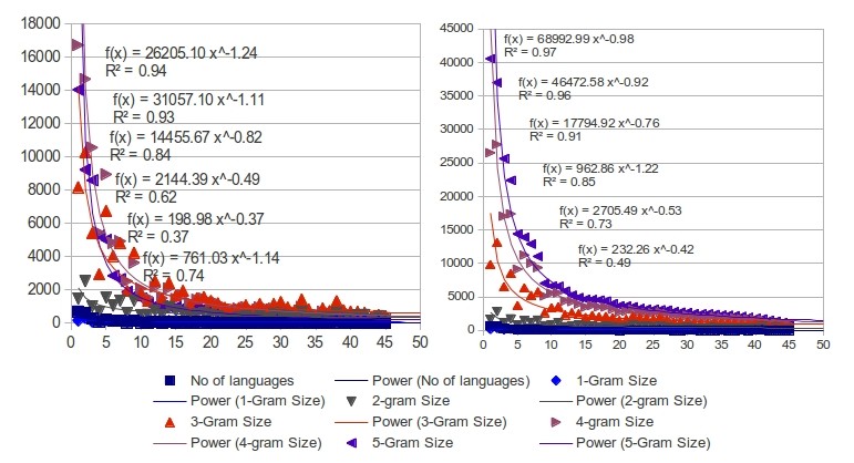
Figure 3: N-gram profiles fitted to a power law.

Language family	NOL	3-gram	4-gram	5-gram	Language family	NOL	3-gram	4-gram	5-gram
Austronesian	692	9808	26527	40561	Macro-Ge	20	1813	2684	3180
Niger-Congo	615	13085	27766	36987	Sepik	22	1677	2623	3144
Trans-NewGuinea	275	6492	17051	25634	Tai-Kadai	42	2036	2723	3077
Afro-Asiatic	201	8456	17403	22403	Chibchan	16	1522	2484	3035
Australian	104	3690	9143	14401	WestPapuan	14	1244	2203	2806
Indo-European	139	6320	11252	13896	EasternTrans-Fly	4	1300	2166	2729
Nilo-Saharan	123	5224	10046	12891	Dravidian	24	1376	2238	2674
Sino-Tibetan	137	5753	9386	11043	LakesPlain	17	1142	2010	2518
Arawakan	39	2626	5148	7021	Border	8	1132	1922	2467
Austro-Asiatic	82	3370	5552	6608	South-CentralPapuan	6	1074	1878	2464
Oto-Manguean	69	3522	5607	6579	Penutian	14	1326	2017	2384
Uto-Aztecan	43	2318	4395	5873	Panoan	15	1192	1915	2288
Altaic	46	2634	4304	5248	Witotoan	7	1185	1847	2264
Salishan	16	2492	3944	4903	Hokan	14	1253	1864	2192
Algic	19	1922	3466	4643	Quechuan	22	1101	1734	2093
Tupi	46	2250	3722	4619	Siouan	11	1131	1674	1952
Torricelli	21	2011	3518	4523	Na-Dene	15	1225	1637	1810
Mayan	48	2083	3485	4386	Hmong-Mien	15	1246	1563	1717
Tucanoan	18	1880	3162	3979	Totonacan	10	679	1139	1510
Ramu-LowerSepik	14	1491	2738	3676	Khoisan	12	995	1265	1377
Carib	20	1662	2868	3649	Sko	12	775	1068	1179
NorthCaucasian	29	2180	3158	3537	Mixe-Zoque	12	625	897	1028
Uralic	23	1896	2818	3284

Table 2: The number of languages (NOL), 3-gram, 4-gram and 5-gram profiles for 45 language families.

As we have shown above, the correlation of $N$-gram distribution to language family size improves with increasing $N$ (for $N=1-5$). This is a kind of behavior familiar from corpus studies of word distributions Baayen, (2001), where closed-class items – typically function words – yield distributions similar to the $1$-grams (phonemes) in this study, whereas open-class words display typical power-law behavior for all corpus sizes, just like the $3$–$5$-grams in this study. We take this as an indication that we are on the right track, investigating a genuine linguistic phenomenon. We also test if the genus size across the world’s languages displays a power-law like behavior. A genus (pl. genera) is a language classification unit which contains related languages and is estimated to be 3000–3500 years old. The genus level was originally introduced by Dryer, (2000). We use the genus information given in ASJP database. The current dataset has 538 genera and 5315 word lists. Table 3 shows the results of the application of the statistical tests to different datasets.

Data	$x_{min}$	$\ln(L)$	$n_{tail}$	est	PL	$\alpha\_{sp}$	PLWC	LN	$\exp$	str $\exp$
Hammarström,	1	-1040.715	423	1.667	1041.715	1.36	1040.144	1059.037	1613.822	1039.84	1090.109
ASJP	7	-211.167	43	1.633	212.167	1.22	209.791	209.137	224.509	209.409	210.587
WALS genus	5	-720.257	193	1.898	721.257	1.26	714.354	714.95	747.291	714.197	708.282
1-grams	51	-166.455	35	2.965	167.455	0.37	167.193	168.004	167.56	167.193	167.43
2-grams	367	-239.206	35	2.844	240.206	0.49	239.892	241.277	241.34	239.92	241.153
3-grams	762	-303.22	37	2.262	304.22	0.82	303.293	305.221	308.871	303.323	306.022
4-grams	270	-387.603	45	1.638	388.603	1.11	383.994	382.972	390.789	383.436	384.73
5-grams	173	-340.531	41	1.605	341.531	1.24	337.376	335.605	343.885	336.558	337.789
2-grams†	506	-188.941	27	3.047	189.941	0.53	189.894	191.251	190.82	189.934	191.04
3-grams †	1074	-342.859	41	2.395	343.859	0.76	343.198	345.588	348.941	343.245	346.15
4-grams†	1734	-346.368	38	2.196	347.368	0.92	346.475	348.748	354.397	346.507	350.041
5-grams †	2093	-357.069	38	2.137	358.069	0.98	357.296	359.594	366.483	357.339	361.106

Table 3: The first three rows correspond to the language size data of Hammarström, (2010), ASJP data (from Table 2) and genera sizes. Columns 2–5 correspond to the estimated parameters in a power law. Column 5 shows the AIC value for a power law. Column 6 shows the _sp estimated by a standard spreadsheet package. The remaining columns correspond to the AIC values for the other candidate distributions. The last four rows show the fit of each $n$-gram profile leading upto $5$ and are indicated by a †. For each dataset, the best fit model is indicated in bold. Here, the common factor $2$ is not included in the AIC computation. All the above results are computed using the power-law python package Alstott, (2012).

Judging by AIC, none of the classification unit datasets follow a power-law distribution. It is important to notice that the _est widely differs from _sp. As demonstrated by Clauset et al., (2009), there can be a large difference when estimating for small datasets of size $\leq 50$. Only the $2-5$-gram profiles follow a power-law with cutoff model ascertained by the lowest AIC value. Interestingly, $n_{tail}$ values are highest for $n=3$ followed by $4$ and $5$. The value of for a power law is typically between 2 and 3. The values of _est for $N$-gram profile also lie between 2 and 3.

Data	PLWC	LN	$\exp$	str $\exp$
Hammarström,	$-$0.0	0.046	0.0	$-$0.005	0.087
ASJP	$-$0.012	$-$0.006	0.101	$-$0.004	$-$0.31
genus	$-$0.018	$-$0.065	0.129	$-$0.009	$-$0.063
1-grams	$-$0.097	$-$0.802	0.962	$-$0.104	$-$0.48
2-grams	$-$0.109	0.969	0.613	$-$0.133	$-$0.972
3-grams	$-$0.086	0.999	0.157	$-$0.099	0.684
4-grams	$-$0.002	$-$0.003	0.7	$-$0.001	$-$0.021
5-grams	$-$0.001	$-$0.001	0.668	$-$0.0	$-$0.011
2-grams†	$-$0.168	0.849	0.619	$-$0.194	0.936
3-grams†	$-$0.093	0.727	0.13	$-$0.097	0.53
4-grams†	$-$0.096	0.851	0.056	$-$0.097	0.43
5-grams†	$-$0.099	0.789	0.035	$-$0.09	0.357

Table 4: The table shows the results of the likelihood-ratio test for comparing the power law with the rest of candidate distributions. The $-$ sign indicates the test favoring the candidate model than the power law model. Each number is the $p$-value and the significance is indicated in bold.

The AIC values in Table 3 suggest that the power-law with cutoff is a better model than power-law for for $N$-gram profiles. We assess this superiority through a likelihood ratio test. The results are given in Table 4. The results suggest that the PLWC is a better fit than PL at a significance criterion $p\leq 0.1$. Interestingly, none of the family-size datasets are genuinely power-lawish. They seem to belong to other “heavy-tailed” distributions. Incidentally, Hammarström,’s dataset – covering more than 7000 languages – fits better to a stretched exponential model than a power-law distribution.

Even though this study shows that phoneme $N$-gram profiles closely mirror the power-law-with-cutoff behavior, it raises more questions than it answers about the use of $N$-gram distributions in linguistic research, such as:

• Is the $N$-gram distribution an effect strictly connected with genetic relatedness among the languages, or simply an effect of the number of languages in a group (regardless of whether they are related or not)?

• We answer this question through the following procedure:

  1. For a family size $s$, make a random sample of languages of size $s$.

  2. Compute the $N$-gram profiles.

  Repeat steps $1-2$ for all family sizes and plot the $N$-gram profile sizes. The results are shown in Figure 4(a). All the $r^{2}$ values are in the range of $0.68$ to $0.75$. This experiment suggests that the $N$-gram distribution is related to genetic relatedness and not an effect of a sample size.

• If the effect is genetic, can the size of the family be predicted from $N$-gram profiles of smaller samples than the full family? (This could be very useful.)

• We answer this question through the following procedure:

  1. For a family of size $s$, create a random language sample of size $i$, where $1\leq i\leq s$.

  2. Compute the $N$-gram profiles for each random sample.

  3. Repeat steps $1-2$ for $10$ iterations and compute the average size of a $N$-gram profile for each $i$.

  Repeat the steps $1-3$ for all $i$. The results of this experiment for $s=104$ (Australian family) is shown in Figure 4(b). Figure 4(b) shows the plot for the average number of $N$-gram types vs. the size of language sample. All $N$-gram curves (except $1$ and $2$) seems to be increasing monotonically and not stabilizing after a particular sample size. Only $1$-grams and $2$-grams tend to stabilize with respect to sample size. The $N$-gram curves for other language families also follow the same trend. These results suggest that the $N$-grams ($N\geq 3$) of smaller samples cannot be used to predict the full family size.

(a) Random samples.

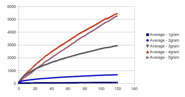
(b) Average $N$-gram profile size

4   Conclusion

In this paper, we tested if the language units of the three classifications obey a power law. We find that the three datasets are not well modeled by a power law model. We then tested if the $N$-gram profiles follow a power law and observed that they actually follow a power-law with cutoff distribution. Finally, we posed two questions about the utility of $N$-grams for historical linguistics and found that $N$-grams do not pass the test.

References

- Alstott, (2012) Alstott, J. (2012). powerlaw Python package. http://pypi.python.org/pypi/powerlaw.
- Baayen, (1991) Baayen, H. (1991). A stochastic process for word frequency distributions. In Proceedings of the 29th annual meeting on Association for Computational Linguistics, pages 271–278. Association for Computational Linguistics.
- Baayen, (2001) Baayen, R. H. (2001). Word frequency distributions. Kluwer Academic Publishers, Dordrecht.
- Campbell and Poser, (2008) Campbell, L. and Poser, W. J. (2008). Language classification: History and method. Cambridge University Press, Cambridge.
- Clauset et al., (2009) Clauset, A., Shalizi, C., and Newman, M. (2009). Power-law distributions in empirical data. SIAM review, 51(4):661–703.
- Cysouw, (2010) Cysouw, M. (2010). On the probability distribution of typological frequencies. In Proceedings of the 10th and 11th Biennial conference on The mathematics of language, MOL’07/09, pages 29–35, Berlin, Heidelberg. Springer-Verlag.
- Dryer, (2000) Dryer, M. S. (2000). Counting genera vs. counting languages. Linguistic Typology, 4:334–350.
- Dunning, (1993) Dunning, T. (1993). Accurate methods for the statistics of surprise and coincidence. Computational Linguistics, 19(1):61–74.
- Evert and Baroni, (2007) Evert, S. and Baroni, M. (2007). zipfr: Word frequency distributions in r. In Proceedings of the 45th Annual Meeting of the ACL on Interactive Poster and Demonstration Sessions, pages 29–32. Association for Computational Linguistics.
- Hammarström, (2010) Hammarström, H. (2010). A full-scale test of the language farming dispersal hypothesis. Diachronica, 27(2):197–213.
- Haspelmath et al., (2011) Haspelmath, M., Dryer, M. S., Gil, D., and Comrie, B. (2011). WALS online. Munich: Max Planck Digital Library. http://wals.info.
- Jäger, (2012) Jäger, G. (2012). Power laws and other heavy-tailed distributions in linguistic typology. Advances in Complex Systems, 15(03/04).
- Lewis, (2009) Lewis, P. M., editor (2009). Ethnologue: Languages of the World. SIL International, Dallas, TX, USA, Sixteenth edition.
- Maslova, (2008) Maslova, E. (2008). Meta-typological distributions. STUF-Language Typology and Universals, 61(3):199–207.
- Swadesh, (1955) Swadesh, M. (1955). Towards greater accuracy in lexicostatistic dating. International Journal of American Linguistics, 21(2):121–137.
- Wichmann, (2005) Wichmann, S. (2005). On the power-law distribution of language family sizes. Journal of Linguistics, 41(1):117–131.
- Wichmann et al., (2011) Wichmann, S., Müller, A., Velupillai, V., Wett, A., Brown, C. H., Molochieva, Z., Sauppe, S., Holman, E. W., Brown, P., Bishoffberger, J., Bakker, D., List, J.-M., Egorov, D., Belyaev, O., Urban, M., Mailhammer, R., Geyer, H., Beck, D., Korovina, E., Epps, P., Valenzuela, P., Grant, A., and Hammarström, H. (2011). The ASJP database version 14. http://email.eva.mpg.de/ wichmann/listss14.zip.
- Zipf, (1935) Zipf, G. K. (1935). The psycho-biology of language. Houghton Mifflin, Boston.