Learning Parametric Dictionaries for
Signals on Graphs

Abstract

In sparse signal representation, the choice of a dictionary often involves a tradeoff between two desirable properties – the ability to adapt to specific signal data and a fast implementation of the dictionary. To sparsely represent signals residing on weighted graphs, an additional design challenge is to incorporate the intrinsic geometric structure of the irregular data domain into the atoms of the dictionary. In this work, we propose a parametric dictionary learning algorithm to design data-adapted, structured dictionaries that sparsely represent graph signals. In particular, we model graph signals as combinations of overlapping local patterns. We impose the constraint that each dictionary is a concatenation of subdictionaries, with each subdictionary being a polynomial of the graph Laplacian matrix, representing a single pattern translated to different areas of the graph. The learning algorithm adapts the patterns to a training set of graph signals. Experimental results on both synthetic and real datasets demonstrate that the dictionaries learned by the proposed algorithm are competitive with and often better than unstructured dictionaries learned by state-of-the-art numerical learning algorithms in terms of sparse approximation of graph signals. In contrast to the unstructured dictionaries, however, the dictionaries learned by the proposed algorithm feature localized atoms and can be implemented in a computationally efficient manner in signal processing tasks such as compression, denoising, and classification.

I Introduction

Graphs are flexible data representation tools, suitable for modeling the geometric structure of signals that live on topologically complicated domains. Examples of signals residing on such domains can be found in social, transportation, energy, and sensor networks[1]. In these applications, the vertices of the graph represent the discrete data domain, and the edge weights capture the pairwise relationships between the vertices. A graph signal is then defined as a function that assigns a real value to each vertex. Some simple examples of graph signals are the current temperature at each location in a sensor network and the traffic level measured at predefined points of the transportation network of a city. An illustrative example is given in Fig. 1.

We are interested in finding meaningful graph signal representations that (i) capture the most important characteristics of the graph signals, and (ii) are sparse. That is, given a weighted graph and a class of signals on that graph, we want to construct an overcomplete dictionary of atoms that can sparsely represent graph signals from the given class as linear combinations of only a few atoms in the dictionary. An additional challenge when designing dictionaries for graph signals is that in order to identify and exploit structure in the data, we need to account for the intrinsic geometric structure of the underlying weighted graph. This is because signal characteristics such as smoothness depend on the topology of the graph on which the signal resides (see, e.g., [1, Example 1]).

For signals on Euclidean domains as well as signals on irregular data domains such as graphs, the choice of the dictionary often involves a tradeoff between two desirable properties – the ability to adapt to specific signal data and a fast implementation of the dictionary [2]. In the dictionary learning or dictionary training approach to dictionary design, numerical algorithms such as K-SVD [3] and the Method of Optimal Directions (MOD) [4] (see [2, Section IV] and references therein) learn a dictionary from a set of realizations of the data (training signals). The learned dictionaries are highly adapted to the given class of signals and therefore usually exhibit good representation performance. However, the learned dictionaries are highly non-structured, and therefore costly to apply in various signal processing tasks. On the other hand, analytic dictionaries based on signal transforms such as the Fourier, Gabor, wavelet, curvelet and shearlet transforms are based on mathematical models of signal classes (see [5] and [2, Section III] for a detailed overview of transform-based representations in Euclidean settings). These structured dictionaries often feature fast implementations, but they are not adapted to specific realizations of the data. Therefore, their ability to efficiently represent the data depends on the accuracy of the mathematical model of the data.

The gap between the transform-based representations and the numerically trained dictionaries can be bridged by imposing a structure on the dictionary atoms and learning the parameters of this structure. The structure generally reveals various desirable properties of the dictionary such as translation invariance [6], minimum coherence [7] or efficient implementation [8] (see [2, Section IV.E] for a complete list of references). Structured dictionaries generally represent a good trade-off between approximation performance and efficiency of the implementation.

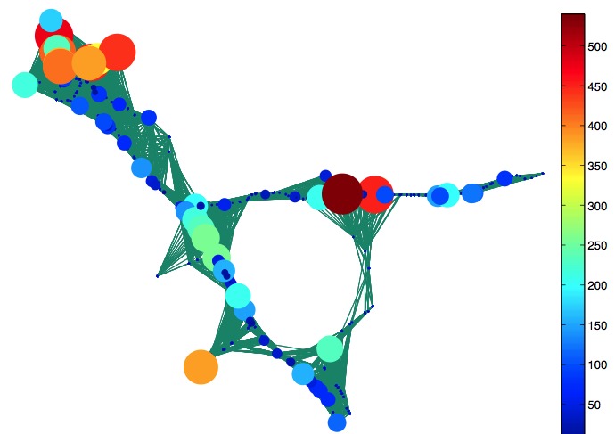
(a) Day 1

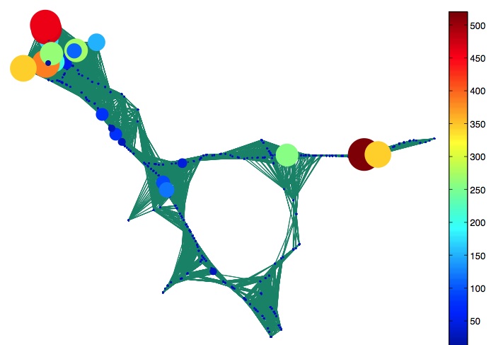
(b) Day 2

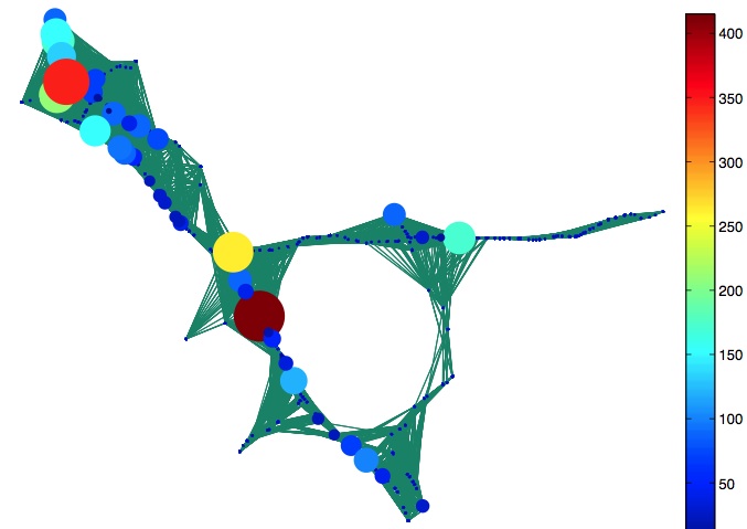
(c) Day 3

Figure 1: Illustrative example: The three signals on the graph are the minutes of bottlenecks per day at different detector stations in Alameda County, California, on three different days. The detector stations are the nodes of the graph and the connectivity is defined based on the GPS coordinates of the stations. Note that all signals consist of a set of localized features positioned on different nodes of the graph.

In this work, we build on our previous work [9] and capitalize on the benefits of both numerical and analytical approaches by learning a dictionary that incorporates the graph structure and can be implemented efficiently. We model the graph signals as combinations of overlapping local patterns, describing localized events or causes on the graph. For example, the evolution of traffic on a highway might be similar to that on a different highway, at a different position in the transportation network. We incorporate the underlying graph structure into the dictionary through the graph Laplacian operator, which encodes the connectivity. In order to ensure the atoms are localized in the graph vertex domain, we impose the constraint that our dictionary is a concatenation of subdictionaries that are polynomials of the graph Laplacian [10]. We then learn the coefficients of the polynomial kernels via numerical optimization. As such, our approach falls into the category of parametric dictionary learning [2, Section IV.E]. The learned dictionaries are adapted to the training data, efficient to store, and computationally efficient to apply. Experimental results demonstrate the effectiveness of our scheme in the approximation of both synthetic signals and graph signals collected from real world applications.

The structure of the paper is as follows. We first highlight some related work on the representation of graph signals in Section II. In Section III, we recall basic definitions related to graphs that are necessary to understand our dictionary learning algorithm. The polynomial dictionary structure and the dictionary learning algorithms are described in Section IV. In Section V, we evaluate the performance of our algorithm on the approximation of both synthetic and real world graph signals. Finally, the benefits of the polynomial structure are discussed in Section VI.

II Related Work

The design of overcomplete dictionaries to sparsely represent signals has been extensively investigated in the past few years. We restrict our focus here to the literature related to the problem of designing dictionaries for graph signals. Generic numerical approaches such as K-SVD [3] and MOD [4] can certainly be applied to graph signals, with signals viewed as vectors in $\mathbb{R}^{N}$. However, the learned dictionaries will neither feature a fast implementation, nor explicitly incorporate the underlying graph structure.

Meanwhile, several transform-based dictionaries for graph signals have recently been proposed (see [1] for an overview and complete list of references). For example, the graph Fourier transform has been shown to sparsely represent smooth graph signals [11]; wavelet transforms such as diffusion wavelets [12], spectral graph wavelets [10], and critically sampled two-channel wavelet filter banks [13] target piecewise-smooth graph signals; and vertex-frequency frames [14, 15, 16] can be used to analyze signal content at specific vertex and frequency locations. These dictionaries feature pre-defined structures derived from the graph and some of them can be efficiently implemented; however, they generally are not adapted to the signals at hand. Two exceptions are the diffusion wavelet packets of [17] and the wavelets on graphs via deep learning[18], which feature extra adaptivity.

The recent work in [19] tries to bridge the gap between the graph-based transform methods and the purely numerical dictionary learning algorithms by proposing an algorithm to learn structured graph dictionaries. The learned dictionaries have a structure that is derived from the graph topology, while its parameters are learned from the data. This work is the closest to ours in a sense that both graph dictionaries consist of subdictionaries that are based on the graph Laplacian. However, it does not necessarily lead to efficient implementations as the obtained dictionary is not necessarily a smooth matrix function (see, e.g., [20] for more on matrix functions) of the graph Laplacian matrix.

Finally, we remark that the graph structure is taken into consideration in [21], not explicitly into the dictionary but rather in the sparse coding coefficients. The authors use the graph Laplacian operator as a regularizer in order to impose that the obtained sparse coding coefficients vary smoothly along the geodesics of the manifold that is captured by the graph. However, the obtained dictionary does not have any particular structure. None of the previous works are able to design dictionaries that provide sparse representations, particularly adapted to a given class of graph signals, and have efficient implementations. This is exactly the objective of our work, where a structured graph signal dictionary is composed of multiple polynomial matrix functions of the graph Laplacian.

III Preliminaries

In this section, we briefly overview a few basic definitions for signals on graphs. A more complete description of the graph signal processing framework can be found in [1]. We consider a weighted and undirected graph $\mathcal{G}=({\mathcal{V}},{\mathcal{E}},W)$ where ${\mathcal{V}}$ and ${\mathcal{E}}$ represent the vertex and edge sets of the graph, and $W$ represents the matrix of edge weights, with $W_{ij}$ denoting the weight of an edge connecting vertices $i$ and $j$. We assume that the graph is connected. The graph Laplacian operator is defined as $L=D-W$, where $D$ is the diagonal degree matrix [22]. The normalized graph Laplacian is defined as ${\mathcal{L}}=D^{-\frac{1}{2}}LD^{-\frac{1}{2}}$. Throughout the paper, we use the normalized graph Laplacian eigenvectors as the Fourier basis in order to avoid some numerical instabilities that arise when taking large powers of the combinatorial graph Laplacian. Both operators are real symmetric matrices and they have a complete set of orthonormal eigenvectors with corresponding nonnegative eigenvalues. We denote the eigenvectors of the normalized graph Laplacian by $\chi=[\chi_{1},\chi_{2},...,\chi_{N}]$, and the spectrum of eigenvalues by

$$\sigma({\mathcal{L}}):=\Bigl{\{}0=\lambda_{0}<\lambda_{1}\leq\lambda_{2}\leq...\leq\lambda_{N-1}\leq 2\Bigr{\}}.$$

A graph signal $y$ in the vertex domain is a real-valued function defined on the vertices of the graph ${\mathcal{G}}$, such that $y(v)$ is the value of the function at vertex $v\in{\mathcal{V}}$. The spectral domain representation can also provide significant information about the characteristics of graph signals. In particular, the eigenvectors of the Laplacian operators can be used to perform harmonic analysis of signals that live on the graph, and the corresponding eigenvalues carry a notion of frequency [1]. The normalized Laplacian eigenvectors are a Fourier basis, so that for any function $y$ defined on the vertices of the graph, the graph Fourier transform $\hat{y}$ at frequency $\lambda_{\ell}$ is defined as

$$\small{\hat{y}\left(\lambda_{\ell}\right)=\langle y,\chi_{\ell}\rangle=\sum_{n=1}^{N}y(n)\chi^{*}_{\ell}(n),}$$

while the inverse graph Fourier transform is

$$\small{y(n)=\sum_{{\ell}=0}^{N-1}\hat{y}\left(\lambda_{\ell}\right)\chi_{\ell}(n),\quad\forall n\in{\mathcal{V}}.}$$

Besides its use in harmonic analysis, the graph Fourier transform is also useful in defining the translation of a signal on the graph. The generalized translation operator can be defined as a generalized convolution with a Kronecker $\delta$ function centered at vertex $n$ [14, 15]:

$$\small{T_{n}g=\sqrt{N}(g*\delta_{n})=\sqrt{N}\sum_{{\ell}=0}^{N-1}\hat{g}(\lambda_{\ell})\chi_{\ell}^{*}(n)\chi_{\ell}.}$$ (1)

The right-hand side of (1) allows us to interpret the generalized translation as an operator acting on the kernel $\hat{g}(\cdot)$, which is defined directly in the graph spectral domain, and the localization of $T_{n}g$ around the center vertex $n$ is controlled by the smoothness of the kernel $\hat{g}(\cdot)$ [10, 15]. One can thus design atoms $T_{n}g$ that are localized around $n$ in the vertex domain by taking the kernel $\hat{g}(\cdot)$ in (1) to be a smooth polynomial function of degree $K$:

$$\small{\hat{g}(\lambda_{\ell})=\sum_{k=0}^{K}\alpha_{k}\lambda_{\ell}^{k},\quad\ell=0,...,N-1.}$$ (2)

Combining (1) and (2), we can translate a polynomial kernel to each vertex in the graph and generate a set of $N$ localized atoms, which are the columns of

$$Tg=\sqrt{N}\hat{g}({\mathcal{L}})=\sqrt{N}\chi\hat{g}(\Lambda)\chi^{T}=\sqrt{N}\sum_{k=0}^{K}\alpha_{k}{\mathcal{L}}^{k},$$ (3)

where $\Lambda$ is the diagonal matrix of the eigenvalues. Note that the $k^{th}$ power of the Laplacian ${\mathcal{L}}$ is exactly $k$-hop localized on the graph topology [10]; i.e., for the atom centered on node $n$, if there is no $K$-hop path connecting nodes $n$ and $i$, then $(T_{n}g)(i)=0$ . This definition of localization is based on the shortest path distance on the graph and ignores the weights of the edges.

IV Parametric dictionary learning on graphs

Given a set of training signals on a weighted graph, our objective is to learn a structured dictionary that sparsely represents classes of graph signals. We consider a general class of graph signals that are linear combinations of (overlapping) graph patterns positioned at different vertices on the graph. We aim to learn a dictionary that is capable of capturing all possible translations of a set of patterns. We use the definition (1) of generalized translation, and we learn a set of polynomial generating kernels (i.e., patterns) of the form (2) that capture the main characteristics of the signals in the spectral domain. Learning directly in the spectral domain enables us to detect spectral components that exist in our training signals, such as atoms that are supported on selected frequency components. In this section, we describe in detail the structure of our dictionary and the learning algorithm.

IV-A Dictionary Structure

We design a structured graph dictionary ${\mathcal{D}}=[{\mathcal{D}}_{1},{\mathcal{D}}_{2},...,{\mathcal{D}}_{S}]$ that is a concatenation of a set of $S$ subdictionaries of the form

$$\small{{\mathcal{D}}_{s}=\widehat{g_{s}}({\mathcal{L}})=\chi\left(\sum_{k=0}^{K}\alpha_{sk}\Lambda^{k}\right)\chi^{T}=\sum_{k=0}^{K}\alpha_{sk}{{\mathcal{L}}}^{k},}$$ (4)

where $\widehat{g_{s}}(\cdot)$ is the generating kernel or pattern of the subdictionary ${\mathcal{D}}_{s}$. Note that the atom given by column $n$ of subdictionary ${\mathcal{D}}_{s}$ is equal to $\frac{1}{\sqrt{N}}T_{n}g_{s}$; i.e., the polynomial $\widehat{g_{s}}(\cdot)$ of order $K$ translated to the vertex $n$. The polynomial structure of the kernel $\widehat{g_{s}}(\cdot)$ ensures that the resulting atom given by column $n$ of subdictionary ${\mathcal{D}}_{s}$ has its support contained in a $K$-hop neighborhood of vertex $n$ [10, Lemma 5.2].

The polynomial constraint guarantees the localization of the atoms in the vertex domain, but it does not provide any information about the spectral representation of the atoms. In order to control their frequency behavior, we impose two constraints on the spectral representation of the kernels $\left\{\widehat{g_{s}}(\cdot)\right\}_{s=1,2,\ldots,S}$. First, we require that the kernels are nonnegative and uniformly bounded by a given constant $c$. In other words, we impose that $0\leq\widehat{g_{s}}(\lambda)\leq c$ for all $\lambda\in[0,\lambda_{\max}]$, or, equivalently,

$$\small{0\preceq{\mathcal{D}}_{s}\preceq cI,~{}~{}\forall s\in\{1,2,...,S\},}$$ (5)

where $I$ is the $N\times N$ identity matrix. Each subdictionary ${\mathcal{D}}_{s}$ has to be a positive semi-definite matrix whose maximum eigenvalue is upper bounded by $c$.

Second, since the classes of signals under consideration usually contain frequency components that are spread across the entire spectrum, the learned kernels $\left\{\widehat{g_{s}}(\cdot)\right\}_{s=1,2,\ldots,S}$ should also cover the full spectrum. We thus impose the constraint

$$\small{c-\epsilon_{1}\leq\sum_{s=1}^{S}\widehat{g_{s}}(\lambda)\leq c+\epsilon_{2},\quad\forall\lambda\in[0,\lambda_{\max}],}$$ (6)

or equivalently

$$\small{(c-\epsilon_{1})I\preceq\sum_{s=1}^{S}{\mathcal{D}}_{s}\preceq(c+\epsilon_{2})I,}$$ (7)

where $\epsilon_{1},\epsilon_{2}$ are small positive constants. Note that both (5) and (7) are quite generic and do not assume any particular prior on the spectral behavior of the atoms. If we have additional prior information, we can incorporate that prior into our optimization problem by modifying these constraints. For example, if we know that our signals’ frequency content is restricted to certain parts of the spectrum, by choosing $\epsilon_{1}$ close to $c$, we allow the flexibility for our learning algorithm to learn filters covering only these parts and not the entire spectrum.

Finally, the spectral constraints increase the stability of the dictionary. From the constants $c$, $\epsilon_{1}$ and $\epsilon_{2}$, we can derive frame bounds for ${\mathcal{D}}$, as shown in the following proposition.

Proposition 1.

Consider a dictionary ${\mathcal{D}}=[{\mathcal{D}}_{1},{\mathcal{D}}_{2},...,{\mathcal{D}}_{S}]$, where each ${\mathcal{D}}_{s}$ is of the form of ${\mathcal{D}}_{s}=\sum_{k=0}^{K}\alpha_{sk}{{\mathcal{L}}}^{k}$. If the kernels $\left\{\widehat{g_{s}}(\cdot)\right\}_{s=1,2,\ldots,S}$ satisfy the constraints $0\leq\widehat{g_{s}}(\lambda)\leq c$ and $c-\epsilon_{1}\leq\sum_{s=1}^{S}\widehat{g_{s}}(\lambda)\leq c+\epsilon_{2},$ for all $\lambda\in[0,\lambda_{\max}]$ then the set of atoms $\left\{{d_{s,n}}\right\}_{s=1,2,\ldots,S,n=1,2,...,N}$ of ${\mathcal{D}}$ form a frame. For every signal $y\in\mathbb{R}^{N}$,

$$\frac{(c-\epsilon_{1})^{2}}{S}\|y\|^{2}_{2}\leq\sum_{n=1}^{N}\sum_{s=1}^{S}|\langle y,d_{s,n}\rangle|^{2}\leq(c+\epsilon_{2})^{2}\|y\|^{2}_{2}.$$

Proof.

From [16, Lemma 1], which is a slight generalization of [10, Theorem 5.6], we have

$$\sum_{n=1}^{N}\sum_{s=1}^{S}|\langle y,d_{s,n}\rangle|^{2}=\sum_{\ell=0}^{N-1}|\hat{y}(\lambda_{\ell})|^{2}\sum_{s=1}^{S}|\widehat{g_{s}}(\lambda_{\ell})|^{2},~{}~{}\forall\lambda\in\sigma({\mathcal{L}}).$$ (8)

From the constraints on the spectrum of kernels $\left\{\widehat{g_{s}}(\cdot)\right\}_{s=1,2,\ldots,S}$ we have

$$\sum_{s=1}^{S}|\widehat{g_{s}}(\lambda_{\ell})|^{2}\leq\left(\sum_{s=1}^{S}\widehat{g_{s}}(\lambda_{\ell})\right)^{2}\leq(c+\epsilon_{2})^{2},~{}~{}\forall\lambda\in\sigma({\mathcal{L}})$$ (9)

Moreover, from the left side of (7) and the Cauchy-Schwarz inequality, we have

$$\frac{(c-\epsilon_{1})^{2}}{S}\leq\frac{\left(\sum_{s=1}^{S}\widehat{g_{s}}(\lambda_{\ell})\right)^{2}}{S}\leq\sum_{s=1}^{S}|\widehat{g_{s}}(\lambda_{\ell})|^{2},~{}~{}\forall\lambda\in\sigma({\mathcal{L}}).$$ (10)

Combining (8), (9) and (10) yields the desired result. ∎

We remark that if we alternatively impose that $\sum_{s=1}^{S}|\widehat{g_{s}}(\lambda)|^{2}$ is constant for all $\lambda\in[0,\lambda_{\max}]$, the resulting dictionary ${\mathcal{D}}$ would be a tight frame. However, such a constraint leads to a significantly more difficult optimization problem to learn the dictionary. The constraints (5) and (7) lead to an easier dictionary learning optimization problem, while still providing control on the spectral representation of the atoms and the stability of signal reconstruction with the learned dictionary.

To summarize, the dictionary ${\mathcal{D}}$ is a parametric dictionary that depends on the parameters

$$\left\{\alpha_{sk}\right\}_{s=1,2,\ldots,S;~{}k=1,2,\ldots,K},$$

and the constraints (5) and (7) can be viewed as constraints on these parameters.

IV-B Dictionary Learning Algorithm

Given a set of training signals $Y=[y_{1},y_{2},...,y_{M}]\in\mathbb{R}^{N\times M}$, all living on the weighted graph $\mathcal{G}$, our objective is to learn a graph dictionary ${\mathcal{D}}\in\mathbb{R}^{N\times NS}$ with the structure described in Section IV-A that can efficiently represent all of the signals in $Y$ as linear combinations of only a few of its atoms. Since ${\mathcal{D}}$ has the form (4), this is equivalent to learning the parameters $\left\{\alpha_{sk}\right\}_{s=1,2,\ldots,S;~{}k=1,2,\ldots,K}$ that characterize the set of generating kernels, $\left\{\widehat{g_{s}}(\cdot)\right\}_{s=1,2,\ldots,S}$. We denote these parameters in vector form as $\alpha=[\alpha_{1};...;\alpha_{S}]$, where $\alpha_{s}$ is a column vector with $(K+1)$ entries.

Therefore, the dictionary learning problem can be cast as the following optimization problem:

$$\operatorname*{argmin}_{\alpha\in\mathbb{R}^{(K+1)S},~{}X\in\mathbb{R}^{SN\times M}} \left\{||Y-{\mathcal{D}}X||^{2}_{F}+\mu\|\alpha\|_{2}^{2}\right\}$$ (11)

subject to $$\|x_{m}\|_{0}\leq T_{0},\quad\forall m\in\{1,...,M\},$$

$${\mathcal{D}}_{s}=\sum_{k=0}^{K}\alpha_{sk}{\mathcal{L}}^{k},\quad\forall s\in\{1,2,...,S\}$$

$$0\preceq{\mathcal{D}}_{s}\preceq c,\quad\forall s\in\{1,2,...,S\}$$

$$(c-\epsilon_{1})I\preceq\sum_{s=1}^{S}{\mathcal{D}}_{s}\preceq(c+\epsilon_{2})I,$$

where ${\mathcal{D}}=[{\mathcal{D}}_{1},{\mathcal{D}}_{2},\ldots,{\mathcal{D}}_{S}]$, $x_{m}$ corresponds to column $m$ of the coefficient matrix $X$, and $T_{0}$ is the sparsity level of the coefficients of each signal. Note that in the objective of the optimization problem (11), we penalize the norm of the polynomial coefficients $\alpha$ in order to (i) promote smoothness in the learned polynomial kernels, and (ii) improve the numerical stability of the learning algorithm.

The optimization problem (11) is not convex, but it can be approximately solved in a computationally efficient manner by alternating between the sparse coding and dictionary update steps. In the first step, we fix the parameters $\alpha$ (and accordingly fix the dictionary ${\mathcal{D}}$ via the structure (4)) and solve

$$\small{\underset{X}{\operatorname{argmin}}||Y-{\mathcal{D}}X||^{2}_{F}\quad\mbox{ subject to }\|x_{m}\|_{0}\leq T_{0}\quad\forall m\in\{1,...,M\},}$$

using orthogonal matching pursuit (OMP) [23], [24], which has been shown to perform well in the dictionary learning literature. Before applying OMP, we normalize the atoms of the dictionary so that they all have a unit norm. This step is essential for the OMP algorithm in order to treat all of the atoms equally. After computing the coefficients $X$, we renormalize the atoms of our dictionary to recover our initial polynomial structure [25, Chapter 3.1.4] and the sparse coding coefficients in such a way that the product ${\mathcal{D}}X$ remains constant. Note that other methods for solving the sparse coding step such as matching pursuit (MP) or iterative soft thresholding could be used as well.

In the second step, we fix the coefficients $X$ and update the dictionary by finding the vector of parameters, $\alpha$, that solves

$$\operatorname*{argmin}_{\alpha\in\mathbb{R}^{(K+1)S}} \left\{||Y-{\mathcal{D}}X||^{2}_{F}+\mu\|\alpha\|_{2}^{2}\right\}$$ (12)

subject to $${\mathcal{D}}_{s}=\sum_{k=0}^{K}\alpha_{sk}{\mathcal{L}}^{k},\quad\forall s\in\{1,2,...,S\}$$

$$0\preceq{\mathcal{D}}_{s}\preceq cI,\quad\forall s\in\{1,2,...,S\}$$

$$(c-\epsilon_{1})I\preceq\sum_{s=1}^{S}{\mathcal{D}}_{s}\preceq(c+\epsilon_{2})I.$$

Problem (12) is convex and can be written as a quadratic program. The details are given in the Appendix A. Algorithm 1 contains a summary of the basic steps of our dictionary learning algorithm.

Since the optimization problem (11) is solved by alternating between the two steps, the polynomial dictionary learning algorithm is not guaranteed to converge to the optimal solution; however, the algorithm converged in all of experiments to a local optimum. Finally, the complexity of our algorithm is dominated by the pre-computation of the eigenvalues of the Laplacian matrix, which we use to enforce the spectral constraints on the kernels. In the dictionary update step, the quadratic program (line 10 of Algorithm 1) can be efficiently solved in polynomial time using optimization techniques such as interior point methods [26] or operator splitting methods (e.g., Alternating Direction Method of Multipliers [27]). The former methods lead to more accurate solutions, while the latter are better suited to solve large scale problems. For the numerical examples in this paper, we use interior point methods to solve the quadratic optimization problem.

Algorithm 1 Parametric Dictionary Learning on Graphs

0:   Input: Signal set $Y$, initial dictionary ${\mathcal{D}}^{(0)}$, target signal sparsity $T_{0}$, polynomial degree $K$, number of subdictionaries $S$, number of iterations $iter$

0:   Output: Sparse signal representations $X$, polynomial coefficients $\alpha$

0:   Initialization: ${\mathcal{D}}={\mathcal{D}}^{(0)}$

0:   for $i=1,2,...,iter$ do:

0:    Sparse Approximation Step:

0:     (a) Scale each atom in ${\mathcal{D}}$ to a unit norm

0:     (b) Solve $\underset{X}{\operatorname{min}}||Y-{\mathcal{D}}X||^{2}_{F}\quad\mbox{ subject to }\|x_{m}\|_{0}\leq T_{0}\quad\forall m\in\{1,...,M\}$

0:     (c) Rescale $X$ and ${\mathcal{D}}$ to recover the polynomial structure

0:    Dictionary Update Step:

0:     Compute the polynomial coefficients $\alpha$ by solving the optimization problem (12), and update the dictionary according to (4)

0:   end for

V Experimental results

In the following experiments, we quantify the performance of the proposed dictionary learning method in the approximation of both synthetic and real data. First, we study the behavior of our algorithm in the synthetic scenario where the signals are linear combinations of a few localized atoms that are placed on different vertices of the graph. Then, we study the performance of our algorithm in the approximation of graph signals collected from real world applications. In all experiments, we compare the performance of our algorithm to the performance of (i) graph-based transform methods such as the spectral graph wavelet transform (SGWT)[10], (ii) purely numerical dictionary learning methods such as K-SVD [3] that treat the graph signals as vectors in $\mathbb{R}^{N}$ and ignore the graph structure, and (iii) the graph-based dictionary learning algorithm presented in [19]. The kernel bounds in (11), if not otherwise specified, are chosen as $c=1$ and $\epsilon_{1}=\epsilon_{2}=0.01$, and the number of iterations in the learning algorithm is fixed to 25. We use the sdpt3 solver [28] in the yalmip optimization toolbox [29] to solve the quadratic problem (12) in the learning algorithm. In order to directly compare the methods mentioned above, we always use orthogonal matching pursuit (OMP) for the sparse coding step in the testing phase, where we first normalize the dictionary atoms to a unit norm. We could alternatively apply iterative soft thresholding to compute the sparse coding coefficients; however, that would require a careful tuning of the stepsize for each of the algorithms. Finally, the average approximation error is set to $\|Y_{test}-{\mathcal{D}}X_{test}\|_{F}^{2}/|Y_{test}|$, where $|Y_{test}|$ is the size of the testing set and $X_{test}$ are the sparse coding coefficients.

V-A Synthetic Signals

We first study the performance of our algorithm for the approximation of synthetic signals. We generate a graph by randomly placing $N=100$ vertices in the unit square. We set the edge weights based on a thresholded Gaussian kernel function so that $W(i,j)=e^{-\frac{[dist(i,j)]^{2}}{2\theta^{2}}}$ if the physical distance between vertices $i$ and $j$ is less than or equal to $\kappa$, and zero otherwise. We fix $\theta=0.9$ and $\kappa=0.5$ in our experiments, and ensure that the graph is connected.

V-A1 Polynomial Generating Dictionary

In our first set of experiments, to construct a set of synthetic training signals consisting of localized patterns on the graph, we use a generating dictionary that is a concatenation of $S=4$ subdictionaries. Each subdictionary is a fifth order ($K=5$) polynomial of the graph Laplacian according to (4) and captures one of the four constitutive components of our signal class. The generating kernels $\left\{\widehat{g_{s}}(\cdot)\right\}_{s=1,2,\ldots,S}$ of the dictionary are shown in Fig. 2(a). We generate the graph signals by linearly combining $T_{0}\leq 4$ random atoms from the dictionary with random coefficients. We then learn a dictionary from the training signals, and we expect this learned dictionary to be close to the known generating dictionary.

We first study the influence of the size of the training set on the dictionary learning outcome. Collecting a large number of training signals can be infeasible in many applications. Moreover, training a dictionary with a large training set significantly increases the complexity of the learning phase, leading to impractical optimization problems. Using our polynomial dictionary learning algorithm with training sets of $M=\{400,600,2000\}$ signals, we learn a dictionary of $S=4$ subdictionaries. To allow some flexibility into our learning algorithm, we fix the degree of the learned polynomials to $K=20$. Comparing Fig. 2(a) to Figs. 2(b), 2(c), and 2(d), we observe that our algorithm is able to recover the shape of the kernels used for the generating dictionary, even with a very small number of training signals. However, the accuracy of the recovery improves as we increase the size of the training set. To quantify the improvement, we define the mean SNR of the learned kernels as $\frac{1}{S}\sum_{s=1}^{S}-20\log(\|\widehat{g_{s}}(\Lambda)-\widehat{g_{s}}^{{}^{\prime}}(\Lambda)\|_{2})$, where $\widehat{g_{s}}(\Lambda)$ is the true pattern of Fig. 2(a) for the subdictionary ${\mathcal{D}}_{s}$ and $\widehat{g_{s}}^{{}^{\prime}}(\Lambda)$ is the corresponding pattern learned with our polynomial dictionary algorithm. The SNR values that we obtain are $\{4.9,5.3,14.9\}$ for $M=\{400,600,2000\}$, respectively.

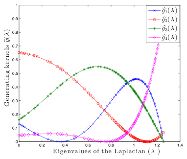
(a) Kernels of the generating dictionary

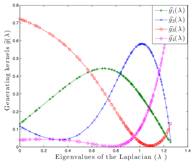
(b) Learned kernels with $M=400$

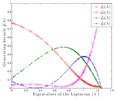
(c) Learned kernels with $M=600$

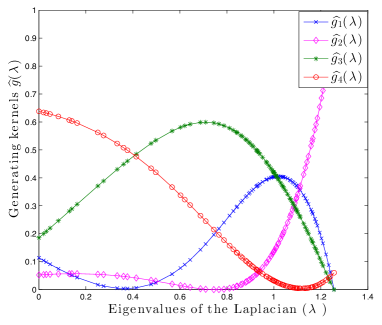
(d) Learned kernels with $M=2000$

Figure 2: Comparison of the kernels learned by the polynomial dictionary learning algorithm to the generating kernels $\left\{\widehat{g_{s}}(\cdot)\right\}_{s=1,2,\ldots,S}$ (shown in (a)) for $M=400$, $M=600$ and $M=2000$ training signals.

Next, we generate 2000 testing signals using the same method as for the the construction of the training signals. We then study the effect of the size of the training set on the approximation of the testing signals with atoms from our learned dictionary. Fig. 3 illustrates the results for three different sizes of the training set and compares the approximation performance to that of other learning algorithms. Each point in the figure is the average of 20 random runs with different realizations of the training and testing sets. We first observe that the approximation performance of the polynomial dictionary is always better than that of SGWT, which demonstrates the benefits of the learning process. The improvement is attributed to the fact that the SGWT kernels are designed a priori, while our algorithm learns the shape of the kernels from the data.

We also see that the performance of K-SVD depends on the size of the training set. Recall that K-SVD is blind to the graph structure, and is therefore unable to capture translations of similar patterns. In particular, we observe that when the size of the training set is relatively small, as in the case of $M=\{500,600\}$, the approximation performance of K-SVD significantly deteriorates. It slightly improves when the number of training signals increases (i.e., $M=2000$). Our polynomial dictionary however shows much more stable performance with respect to the size of the training set. We note two reasons that may underly the better performance of our algorithm, as compared to K-SVD. First, K-SVD tends to learn atoms that sparsely approximate the signal on the whole graph, rather than to extract common features that appear in different neighborhoods. As a result, the atoms learned by K-SVD tend to have a global support on the graph, and K-SVD shows poor performance in the datasets containing many localized signals. An example of the atomic decomposition of a graph signal from the testing set with respect to the K-SVD and the polynomial graph dictionary is illustrated in Fig. 4. Second, even when K-SVD does learn a localized pattern appearing in the training data, it only learns that pattern in that specific area of the graph, and does not assume that similar patterns may appear at other areas of the graph. Of course, as we increase the number of training signals, translated instances of the pattern are more to likely appear in other areas of the graph in the training data, and K-SVD is then more likely to learn atoms containing such patterns in different areas of the graph. On the other hand, our polynomial dictionary learning algorithm learns the patterns in the graph spectral domain, and then includes translated versions of the patterns to all locations in the graph in the learned dictionary, even if some specific instances of the translated patterns do not appear in the training data.

The algorithm proposed in [19] represents some sort of intermediate solution between K-SVD and our algorithm. It learns a dictionary that consists of subdictionaries of the form $\chi\widehat{g_{s}}(\Lambda)\chi^{T}$, where the specific values $\widehat{g_{s}}(\lambda_{0}),\widehat{g_{s}}(\lambda_{1}),\ldots,\widehat{g_{s}}(\lambda_{N-1})$ are learned, rather than learning a continuous kernel $\widehat{g_{s}}(\cdot)$ and evaluating it at the $N$ discrete eigenvalues as we do. As a result, the obtained dictionary is adapted to the graph structure and it contains atoms that are translated versions of the same pattern on the graph. However, the obtained atoms are not guaranteed to be well localized in the graph since the learned discrete values of $\widehat{g_{s}}$ are not necessarily derived from a smooth kernel. Moreover, the unstructured construction of the kernels in the method of [19] leads to more complex implementations, as discussed in Section VI.

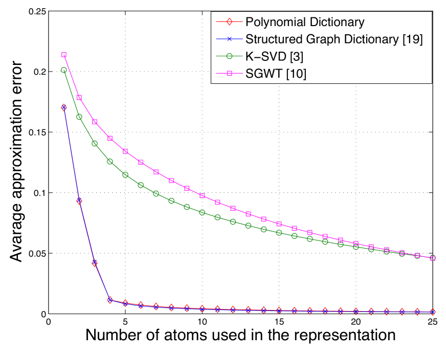
(a) M=400

(b) M=600

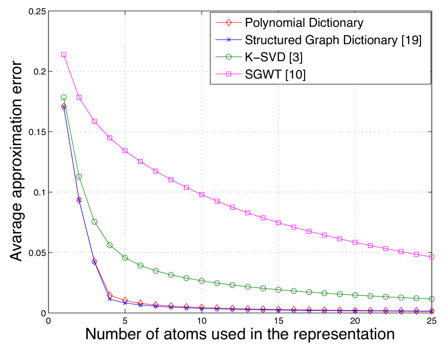
(c) M=2000

Figure 3: Comparison of the learned polynomial dictionary to the SGWT[10], K-SVD [3] and the graph structured dictionary [19] in terms of approximation performance on test data generated from a polynomial generating dictionary, for different sizes of the training set.

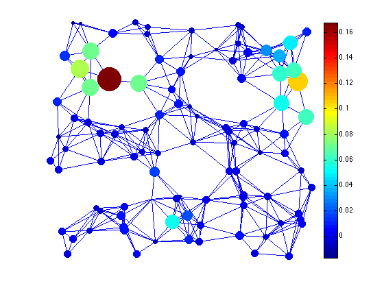
(a) Graph signal

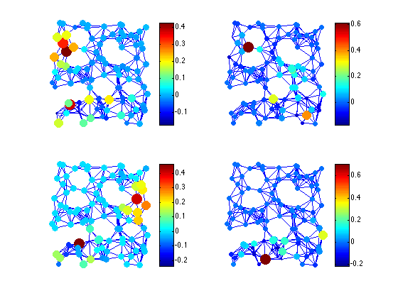
(b) K-SVD

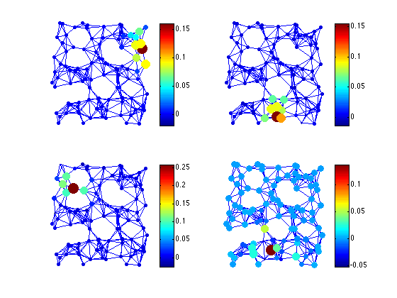
(c) Polynomial dictionary

Figure 4: (a) An example of a graph signal from the testing set and its atomic decomposition with respect to (b) the dictionary learned by K-SVD and (c) the learned polynomial graph dictionary. Note that the K-SVD atoms have a more global support while the polynomial dictionary atoms are localized in specific neighborhoods of the graph.

Finally, we study the resilience of our algorithm to potential noise in the training phase. We generate $M=600$ training signals as linear combinations of $T_{0}\leq 4$ atoms from the generating dictionary and add some Gaussian noise with zero mean and variance $\sigma=0.015$, which corresponds to a noise level with $SNR=4dB$. These training signals are used to learn a polynomial dictionary with polynomials of degree $K=20$. The obtained kernels are shown in Fig. 5. We observe that, even though the training signals are quite noisy, we succeed in learning kernels that preserve the shape of our true noiseless kernels of Fig. 2(a). We then test the performance of our algorithm on a set of 2000 testing signals generated as linear combinations of $T_{0}\leq 4$ atoms from the generating dictionary. The results for different sparsity levels in the OMP approximation are shown in Fig. 5. We observe that both K-SVD and the structured graph dictionary are more sensitive to noise than our polynomial dictionary.

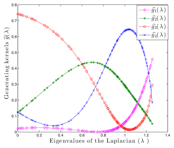
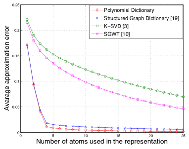
Figure 5: Dictionary learning performance when Gaussian noise is added to the training signals. (a) Kernels learned by the polynomial dictionary. (b) Approximation performance of the polynomial dictionary, SGWT[10], K-SVD [3] and the graph structured dictionary [19] on noiseless testing signals.

V-A2 Non-Polynomial Generating Dictionary

In the next set of experiments, we depart from the idealistic scenario and study the performance of our polynomial dictionary learning algorithm in the more general case when the signal components are not exactly polynomials of the Laplacian matrix. In order to generate training and testing signals, we divide the spectrum of the graph into four frequency bands, defined by the eigenvalues of the graph: $[\lambda_{0}:\lambda_{24}],[(\lambda_{25}:\lambda_{39})\cup(\lambda_{90}:\lambda_{99})],[\lambda_{40}:\lambda_{64}],$ and $[\lambda_{65}:\lambda_{89}]$. We then construct a generating dictionary of $J=400$ atoms, with each atom having a spectral representation that is concentrated exclusively in one of the four bands. In particular, atom $j$ is of the form

$$d_{j}=\widehat{h_{j}}(\mathcal{L})\delta_{n}=\chi\widehat{h_{j}}(\Lambda)\chi^{T}\delta_{n}.$$ (13)

Each atom is generated independently of the others as follows. We randomly pick one of the four bands, randomly generate 25 coefficients uniformly distributed in the range $[0,1]$, and assign these random coefficients to be the diagonal entries of $\widehat{h_{j}}(\Lambda)$ corresponding to the indices of the chosen spectral band. The rest of the values in $\widehat{h_{j}}(\Lambda)$ are set to zero. The atom is then centered on a vertex $n$ that is also chosen randomly. Note that the obtained atoms are not guaranteed to be well localized in the vertex domain since the discrete values of $\widehat{h_{j}}(\Lambda)$ are chosen randomly and are not derived from a smooth kernel. Therefore, the atoms of the generating dictionary do not exactly match the signal model assumed by our dictionary design algorithm. Finally, we generate the training signals by linearly combining (with random coefficients) $T_{0}\leq 4$ random atoms from the generating dictionary.

We first verify the ability of our dictionary learning algorithm to recover the spectral bands that are used in the synthetic generating dictionary. We fix the number of training signals to $M=600$ and run our dictionary learning algorithm for four different degree values of the polynomial, i.e., $K=\{5,10,20,25\}$. The kernels $\left\{\widehat{g_{s}}(\cdot)\right\}_{s=1,2,3,4}$ obtained for the four subdictionaries are shown in Fig. 6. We observe that for higher values of $K$, the learned kernels are more localized in the graph spectral domain. We further notice that, for $K=\{20,25\}$, each kernel approximates one of the four bands defined in the generating dictionary, similarly to the behavior of classical frequency filters.

In Fig. 7, we illustrate the four learned atoms centered at the vertex $n=1$ (one atom for each subdictionary), with $K=20$. We can see that the support of the atoms adapts to the graph topology. The atoms can be either smoother around a particular vertex, as for example in Fig. 7(c), or more localized, as in Fig. 7(a). Comparing Figs. 6(c), and 7, we observe that the localization of the atoms in the graph domain depends on the spectral behavior of the kernels. Note that the smoothest atom on the graph (Fig. 7(c)) corresponds to the subdictionary generated from the kernel that is concentrated on the low frequencies (i.e., $\widehat{g_{3}}(\cdot)$). This is because the graph Laplacian eigenvectors associated with the lower frequencies are smoother with respect to the underlying graph topology, while those associated with the larger eigenvalues oscillate more rapidly [1].

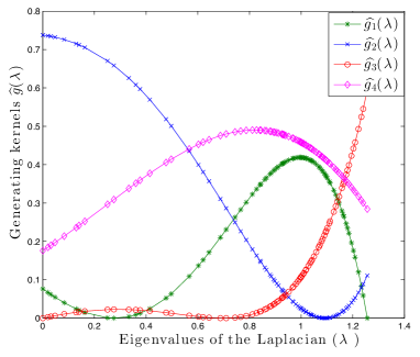
(a) $K=5$

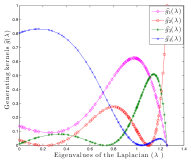
(b) $K=10$

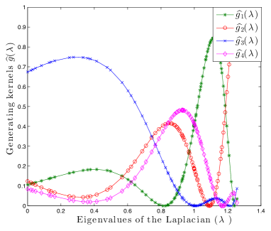
(c) $K=20$

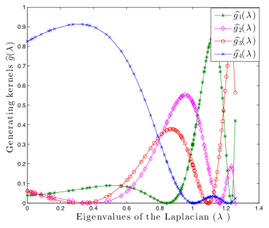
(d) $K=25$

Figure 6: Kernels $\left\{\widehat{g_{s}}(\cdot)\right\}_{s=1,2,3,4}$ learned by the polynomial dictionary algorithm for (a) $K=5$, (b) $K=10$, (c) $K=20$ and (d) $K=25$.

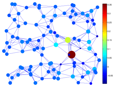
(a) $\widehat{g_{1}}({\mathcal{L}})\delta_{1}$

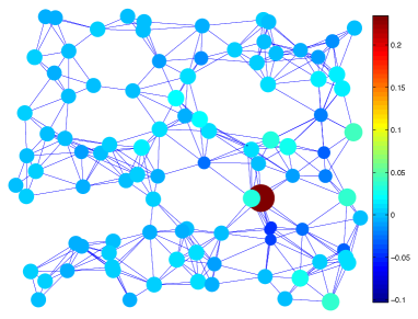
(b) $\widehat{g_{2}}({\mathcal{L}})\delta_{1}$

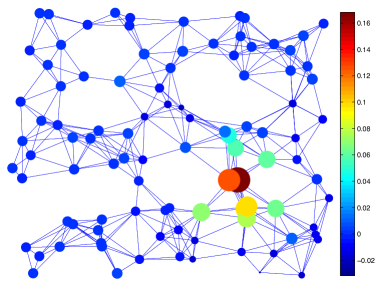
(c) $\widehat{g_{3}}({\mathcal{L}})\delta_{1}$

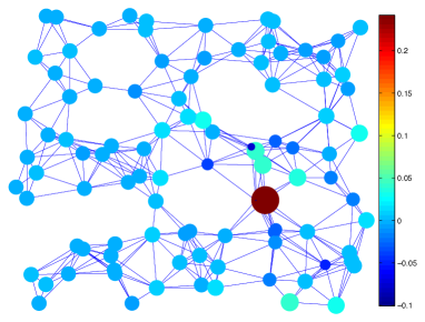
(d) $\widehat{g_{4}}({\mathcal{L}})\delta_{1}$

Figure 7: Learned atoms centered on vertex $n=1$, from each of the subdictionaries. The size and the color of each ball indicate the value of the atom in each vertex of the graph.

Next, we test the approximation performance of our learned dictionary on a set of 2000 testing signals generated in exactly the same way as the training signals. Fig. 8 shows that the approximation performance obtained with our algorithm improves as we increase the polynomial degree. This is attributed to two main reasons: (i) by increasing the polynomial degree, we allow more flexibility in the learning process; (ii) a small $K$ implies that the atoms are localized in a small neighborhood and thus more atoms are needed to represent signals with support in different areas of the graph.

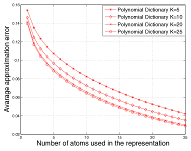
Figure 8: Comparison of the average approximation performance of our learned dictionary on test signals generated by the non-polynomial synthetic generating dictionary, for $K=\{5,10,20,25\}$.

In Fig. 9, we fix $K=20$, and compare the approximation performance of our learned dictionary to that of other dictionaries, with exactly the same setup as we used in Figure 3. We again observe that K-SVD is the most sensitive to the size of the training data, for the same reasons explained earlier. Since the kernels used in the generating dictionary in this case do not match our polynomial model, the structured graph dictionary learning algorithm of [19] has more flexibility to learn the non-smooth generating kernels and therefore generally achieves better approximation. Nonetheless, the approximation performance of our learned dictionary is competitive, especially for smaller training sets, and the learned dictionary is more computationally efficient to implement. For a fairer comparison of approximation performance, we fit an order $K=20$ polynomial function to the discrete values $\widehat{g_{s}}$ learned with the algorithm of [19]. We observe that our polynomial dictionary outperforms the polynomial approximation of the dictionary learned by [19] in terms of approximation performance.

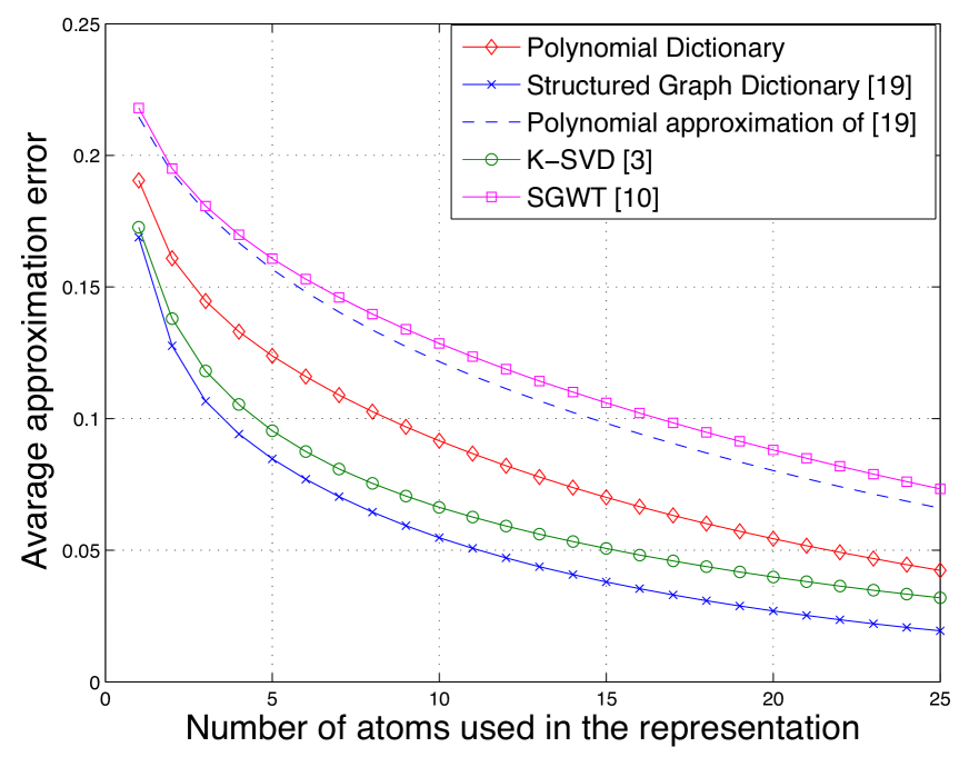
(a) M=400

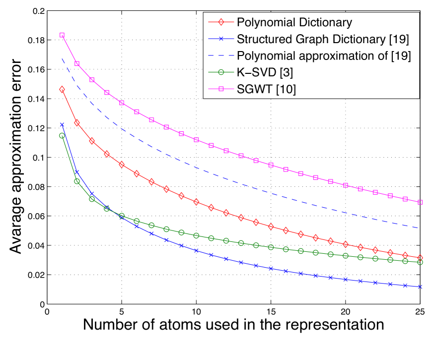
(b) M=600

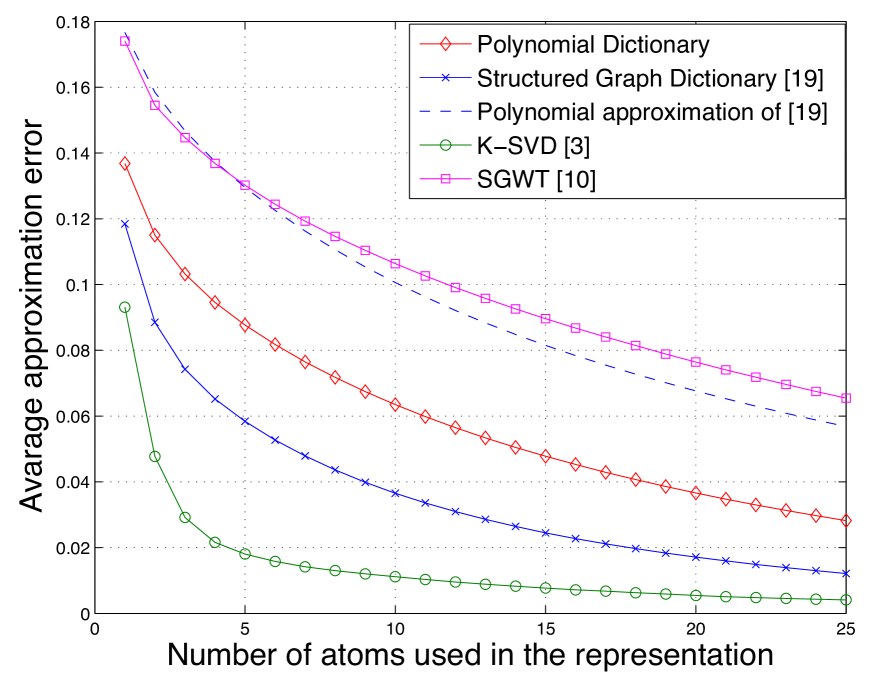
(c) M=2000

Figure 9: Comparison of the learned polynomial dictionary to the SGWT[10], K-SVD [3] and the graph structured dictionary [19] and its polynomial approximation in terms of approximation performance on test data generated from a non-polynomial generating dictionary, for different sizes of the training set.

V-A3 Generating Dictionary Focused on Specific Frequency Bands

In the final set of experiments, we study the behavior of our algorithm in the case when we have the additional prior information that the training signals do not cover the entire spectrum, but are concentrated only in some bands that are not known a priori. In order to generate the training signals, we choose only two particular frequency bands, defined by the eigenvalues of the graph: $[\lambda_{0}:\lambda_{9}]$ and $[\lambda_{89}:\lambda_{99}]$, which correspond to the values $[0:0.275]$ and $[1.174:1.256]$, respectively. We construct a generating dictionary of $J=400$ atoms, with each atom concentrated in only one of the two bands and generated according to (13). The training signals ($M=600$) are then constructed by linearly combining $T_{0}\leq 4$ atoms from the generating dictionary. We set $K=20$ and $\epsilon_{1}=c$ in order to allow our polynomial dictionary learning algorithm the flexibility to learn kernels that are supported only on specific frequency bands. The learned kernels are illustrated in Fig. 10. We observe that the algorithm is able to detect the spectral components that exist in the training signals since the learned kernels are concentrated only in the two parts of the spectrum to which the atoms of the generating dictionary belong.

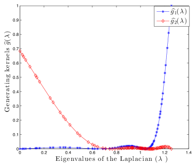
Figure 10: Kernels $\left\{\widehat{g_{s}}(\cdot)\right\}_{s=1,2}$ learned by the polynomial dictionary algorithm from a set of training signals that are supported in only two particular bands of the spectrum. The bands are defined by the eigenvalues of the graph $[\lambda_{0}:\lambda_{9}]$ and $[\lambda_{89}:\lambda_{99}]$, which correspond to the values $[0:0.275]$ and $[1.174:1.256]$ respectively.

V-B Approximation of Real Graph Signals

After examining the behavior of the polynomial dictionary learning algorithm for synthetic signals, we illustrate the performance of our algorithm in the approximation of localized graph signals from real world datasets. In particular, we examine the following three datasets.

• Flickr Dataset: We consider the daily number of distinct Flickr users that took photos at different geographical locations around Trafalgar Square in London, between January 2010 and June 2012 [30]. Each vertex of the graph represents a geographical area of $10\times 10$ meters. The graph is constructed by assigning an edge between two locations when the distance between them is shorter than 30 meters, and the edge weight is set to be inversely proportional to the distance. We then remove edges whose weight is below a threshold in order to obtain a sparse graph. The number of vertices of the graph is $N=245$. We set $S=2$ and $K=10$ in our dictionary learning algorithm. We have a total of 913 signals, and we use 700 of them for training and the rest for testing.

• Traffic Dataset: We consider the daily bottlenecks in Alameda County in California between January 2007 and May 2013. The data are part of the Caltrans Performance Measurement System (PeMS) dataset that provides traffic information throughout all major metropolitan areas of California [31]. In particular, the nodes of the graph consist of $N=439$ detector stations where bottlenecks were identified over the period under consideration. The graph is designed by connecting stations when the distance between them is smaller than a threshold of $\theta=0.08$ which corresponds to approximately 13 kilometres. The distance is set to be the Euclidean distance of the GPS coordinates of the stations and the edge weights are set to be inversely proportional to the distance. A bottleneck could be any location where there is a persistent drop in speed, such as merges, large on-ramps, and incidents. The signal on the graph is the average length of the time in minutes that a bottleneck is active for each specific day. In our experiments, we fix the maximum degree of the polynomial to $K=10$ and we learn a dictionary consisting of $S=2$ subdictionaries. We use the signals in the period between January 2007 and December 2010 for training and the rest for testing. For computational issues, we normalize all the signals with respect to the norm of the signal with maximum energy.

• Brain Dataset: We consider a set of fMRI signals acquired on five different subjects [32], [33]. For each subject, the signals have been preprocessed into timecourses of $N=90$ brain regions of contiguous voxels, which are determined from a fixed anatomical atlas, as described in [33]. The timecourses for each subject correspond to 1290 different graph signals that are measured while the subject is in different states, such as completely relaxing, in the absence of any stimulation or passively watching small movie excerpts. For the purpose of this paper, we treat the measurements at each time as an independent signal on the 90 vertices of the brain graph. The anatomical distances between regions of the brain are approximated by the Euclidean distance between the coordinates of the centroids of each region, the connectivity of the graph is determined by assigning an edge between two regions when the anatomical distance between them is shorter than 40 millimetres, and the edge weight is set to be inversely proportional to the distance. We then apply our polynomial dictionary learning algorithm in order to learn a dictionary of atoms representing brain activity across the network at a fixed point in time. We use the graph signals from the timecourses of two subjects as our training signals and we learn a dictionary of $S=2$ subdictionaries and a maximum polynomial degree of $K=15$. We use the graph signals from the remaining three timecourses to validate the performance of the learned dictionary. As in the previous dataset, we normalize all of the graph signals with respect to the norm of the signal with maximum energy.

Fig. 11 shows the approximation performance of the learned polynomial dictionaries for the three different datasets. The behavior is similar in all three datasets, and also similar to results on the synthetic datasets in the previous section. In particular, the data-adapted dictionaries clearly outperform the SGWT dictionary in terms of approximation error on test signals, and the localized atoms of the learned polynomial dictionary effectively represent the real graph signals.

In Fig. 12, we illustrate the six most used atoms after applying OMP for the sparse decomposition of the testing signals from the brain dataset in the learned K-SVD dictionary and our learned polynomial dictionary. Note that in Fig. 12(b), the polynomial dictionary consists of localized atoms with supports concentrated on the close neighborhoods of different vertices, which can lead to poor approximation performance at low sparsity levels. However, as the sparsity level increases, the localization property clearly becomes beneficial. As was the case in the synthetic datasets, the learned polynomial dictionary also has the ability to represent localized patterns that did not appear in the training data, unlike K-SVD. For example, an unexpected event in London could significantly increase the number of pictures taken in the vicinity of a location that was not necessarily popular in the past.

Comparing our algorithm with the one of [19], we observe that the performance of the latter is sometimes better (see Fig. 11(b)) and sometimes worse (see Figs. 11(a), 11(c)). Apart from the differences between the two algorithms that we have already discussed in the previous subsections, one drawback of [19] is the way the dictionary is updated. Specifically, the update of the dictionary is performed block by block, which leads to a local optimum in the dictionary update step. This can lead to worse performance when compared to our algorithm, where all subdictionaries are updated simultaneously.

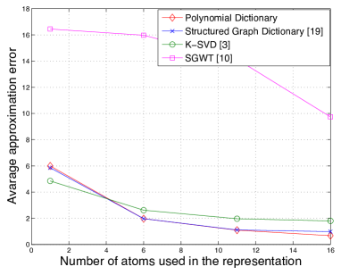
(a) Flickr Dataset

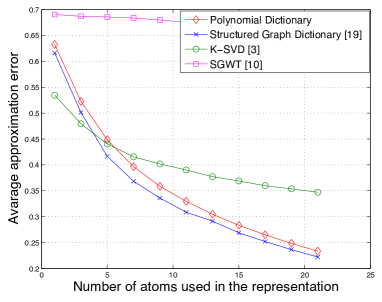
(b) Traffic Dataset

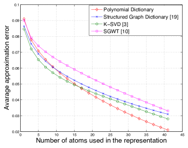
(c) Brain Dataset

Figure 11: Comparison of the learned polynomial dictionaries to the SGWT, K-SVD, and graph structured dictionaries [19] in terms of approximation performance on testing data generated from the (a) Flickr, (b) traffic, and (c) brain datasets, respectively.

(a) K-SVD

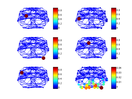
(b) Polynomial Dictionary

Figure 12: Examples of atoms learned from training data from the brain dataset with (a) K-SVD and (b) the polynomial dictionary. The six atoms are the ones that were most commonly included by OMP in the sparse decomposition of the testing signals. Notice that the atoms in (a) have a support that covers the entire graph while the atoms in (b) are localized around a vertex.

VI Computational Efficiency of the Learned Polynomial Dictionary

The structural properties of the proposed class of dictionaries lead to compact representations and computationally efficient implementations, which we elaborate on briefly in this section. First, the number of free parameters depends on the number $S$ of subdictionaries and the degree $K$ of the polynomials. The total number of parameters is $(K+1)S$, and since $K$ and $S$ are small in practice, the dictionary is compact and easy to store. Second, contrary to the non-structured dictionaries learned by algorithms such as K-SVD and MOD, the dictionary forward and adjoint operators can be efficiently applied when the graph is sparse, as is usually the case in practice. Recall from (4) that ${\mathcal{D}}^{T}y=\sum_{s=1}^{S}\sum_{k=0}^{K}\alpha_{sk}{\mathcal{L}}^{k}$. The computational cost of the iterative sparse matrix-vector multiplication required to compute $\{\mathcal{L}^{k}y\}_{k=1,2,...,K}$ is $O(K|{\mathcal{E}}|)$. Therefore, the total computational cost to compute ${\mathcal{D}}^{T}y$ is $O(K|{\mathcal{E}}|+NSK)$. We further note that, by following a procedure similar to the one in [10, Section 6.1], the term ${\mathcal{D}}{\mathcal{D}}^{T}y$ can also be computed in a fast way by exploiting the fact that ${\mathcal{D}}{\mathcal{D}}^{T}y=\sum_{s=1}^{S}\widehat{g_{s}}^{2}(\mathcal{L})y$. This leads to a polynomial of degree $K^{{}^{\prime}}=2K$ that can be efficiently computed. Both operators ${\mathcal{D}}^{T}y$ and ${\mathcal{D}}{\mathcal{D}}^{T}y$ are important components of most sparse coding techniques.

Therefore, these efficient implementations are useful in numerous signal processing tasks, and comprise one of the main advantages of learning structured parametric dictionaries. For example, to find sparse representations of different signals with the learned dictionary, rather than using OMP, we can use iterative soft thresholding [34] to solve the lasso regularization problem [35]. The two main operations required in iterative soft thresholding, ${\mathcal{D}}^{T}y$ and ${\mathcal{D}}^{T}{\mathcal{D}}x$, can both be approximated by the Chebyshev approximation method of [10], as explained in more detail in [36, Section IV.C].

A third computational benefit is that in settings where the data is distributed and communication between nodes of the graph is costly (e.g., a sensor network), the polynomial structure of the learned dictionary enables quantities such as ${\mathcal{D}}^{T}y$, ${\cal D}x$, ${\mathcal{D}}{\mathcal{D}}^{T}y$, and ${\mathcal{D}}^{T}{\mathcal{D}}x$ to be efficiently computed in a distributed fashion using the techniques of [36]. As discussed in [36], this structure makes it possible to implement many signal processing algorithms in a distributed fashion.

VII Conclusion

We proposed a parameterized family of structured dictionaries – namely, unions of polynomial matrix functions of the graph Laplacian – to sparsely represent signals on a given weighted graph, and an algorithm to learn the parameters of a dictionary belonging to this family from a set of training signals on the graph. When translated to a specific vertex, the learned polynomial kernels in the graph spectral domain correspond to localized patterns on the graph. The fact that we translate each of these patterns to different areas of the graph led to sparse approximation performance that was clearly better than that of non-adapted graph wavelet dictionaries such as the SGWT and comparable to or better than that of dictionaries learned by state-of-the art numerical algorithms such as K-SVD. The approximation performance of our learned dictionaries was also more robust to the available size of training data. At the same time, because our learned dictionaries are unions of polynomial matrix functions of the graph Laplacian, they can be efficiently stored and implemented in both centralized and distributed signal processing tasks.

Appendix A

The optimization problem (12) is a quadratic program as it consists of a quadratic objective function and a set of affine constraints. In particular, using (4), the objective function can be written as

$${\small\begin{split}||Y-{\mathcal{D}}X||^{2}_{F}+\mu\|\alpha\|_{2}^{2}&=\sum_{n=1}^{N}\sum_{m=1}^{M}(Y-{\mathcal{D}}X)_{nm}^{2}+\mu\alpha^{T}\alpha\\ &=\sum_{n=1}^{N}\sum_{m=1}^{M}\left(Y-\sum_{s=1}^{S}\sum_{k=0}^{K}\alpha_{sk}{{\mathcal{L}}}^{k}X_{s}\right)_{nm}^{2}+\mu\alpha^{T}\alpha,\end{split}}$$ (14)

where $X_{s}\in\mathbb{R}^{N\times M}$ denotes the rows of the matrix $X$ corresponding to the atoms in the subdictionary ${\mathcal{D}}_{s}$. Let us define the column vector $P_{nm}^{s}\in\mathbb{R}^{(K+1)}$ as

$$\small{P_{nm}^{s}=[({\mathcal{L}}^{0})_{(n,:)}{X_{s}}_{(:,m)};({\mathcal{L}}^{1})_{(n,:)}{X_{s}}_{(:,m)};...;({\mathcal{L}}^{K})_{(n,:)}{X_{s}}_{(:,m)}],}$$

where $({\mathcal{L}}^{k})_{(n,:)}$ is the $n^{th}$ row of the $k^{th}$ power of the Laplacian matrix and ${X_{s}}_{(:,m)}$ is the $m^{th}$ column of the matrix $X_{s}$. We then stack these column vectors into the column vector $P_{nm}\in\mathbb{R}^{S(K+1)}$, which is defined as $P_{nm}=[P_{nm}^{1};P_{nm}^{2};...;P_{nm}^{S}]$. Using this definition of $P_{nm}$, (14) can be written as

$${\small\begin{split}||Y-{\mathcal{D}}X||^{2}_{F}+\mu\|\alpha\|_{2}^{2}&=\sum_{n=1}^{N}\sum_{m=1}^{M}(Y_{nm}-P_{nm}^{T}\alpha)^{2}+\mu\alpha^{T}\alpha\\ &=\sum_{n=1}^{N}\sum_{m=1}^{M}Y_{nm}^{2}-2Y_{nm}P_{nm}^{T}\alpha+\alpha^{T}P_{nm}P_{nm}^{T}\alpha+\mu\alpha^{T}\alpha\\ &=\|Y\|_{F}^{2}-2\left(\sum_{n=1}^{N}\sum_{m=1}^{M}Y_{nm}P_{nm}^{T}\right)\alpha+\alpha^{T}\left(\sum_{n=1}^{N}\sum_{m=1}^{M}P_{nm}P_{nm}^{T}+\mu I_{S(K+1)}\right)\alpha,\end{split}}$$

where $I_{S(K+1)}$ is the $S(K+1)\times S(K+1)$ identity matrix. The matrix $\sum_{n=1}^{N}\sum_{m=1}^{M}P_{nm}P_{nm}^{T}+\mu I$ is positive semidefinite, which implies that our objective is quadratic.

Finally, the optimization constraints can be expressed as affine functions with

$$0\leq I_{S}\otimes B\alpha\leq c\boldsymbol{1}$$

and

$$(c-\epsilon)\boldsymbol{1}\leq\boldsymbol{1}^{T}\otimes B\alpha\leq(c+\epsilon)\boldsymbol{1}~{},$$

where the inequalities are component-wise inequalities, $\boldsymbol{1}$ is the vector of ones, $I_{S}$ is the $S\times S$ identity matrix, and $B$ is the Vandermonde matrix

$$B=\begin{bmatrix}1&\lambda_{0}&\lambda_{0}^{2}\dots\lambda_{0}^{K}\\ 1&\lambda_{1}&\lambda_{1}^{2}\dots\lambda_{1}^{K}\\ \vdots&\vdots&\vdots\\ 1&\lambda_{N-1}&\lambda_{N-1}^{2}\dots\lambda_{N-1}^{K}\\ \end{bmatrix}.$$

Thus, the optimization problem is quadratic and it can be solved efficiently.

References

- [1] D. I Shuman, S. K. Narang, P. Frossard, A. Ortega, and P. Vandergheynst, “The emerging field of signal processing on graphs: Extending high-dimensional data analysis to networks and other irregular domains,” IEEE Signal Process. Mag., vol. 30, no. 3, pp. 83–98, May 2013.
- [2] R. Rubinstein, A. M. Bruckstein, and M. Elad, “Dictionaries for sparse representation modeling,” Proc. of the IEEE, vol. 98, no. 6, pp. 1045 –1057, Apr. 2010.
- [3] M. Aharon, M. Elad, and A. Bruckstein, “K-SVD: An algorithm for designing overcomplete dictionaries for sparse representation,” IEEE Trans. Signal Process., vol. 54, no. 11, pp. 4311–4322, 2006.
- [4] K. Engan, S. O. Aase, and J. H. Husoy, “ Method of optimal directions for frame design,” in Proc. IEEE Int. Conf. Acc., Speech, and Signal Process., Washington, DC, USA, 1999, vol. 5, pp. 2443–2446.
- [5] S. Mallat, A Wavelet Tour of Signal Processing: The Sparse Way, Academic Press, 3rd edition, 2008.
- [6] P. Jost, P. Vandergheynst, S. Lesage, and R. Gribonval, “Motif: An efficient algorithm for learning translation invariant dictionaries,” in Proc. IEEE Int. Conf. Acc., Speech, and Signal Process., Toulouse, France, 2006, vol. 5, pp. 857–860.
- [7] M. Yaghoobi, L. Daudet, and M. E. Davies, “Parametric dictionary design for sparse coding,” IEEE Trans. Signal Process., vol. 57, no. 12, pp. 4800–4810, Dec. 2009.
- [8] R. Rubinstein, M. Zibulevsky, and M. Elad, “Double sparsity: learning sparse dictionaries for sparse signal approximation,” IEEE Trans. Signal Process., vol. 58, no. 3, pp. 1553–1564, 2010.
- [9] D. Thanou, D. I Shuman, and P. Frossard, “Parametric dictionary learning for graph signals,” in Proc. IEEE Glob. Conf. Signal and Inform. Process., Austin, Texas, Dec. 2013.
- [10] D. Hammond, P. Vandergheynst, and R. Gribonval, “Wavelets on graphs via spectral graph theory,” Appl. Comput. Harmon. Anal., vol. 30, no. 2, pp. 129–150, March 2010.
- [11] X. Zhu and M. Rabbat, “Approximating signals supported on graphs,” in Proc. IEEE Int. Conf. Acc., Speech, and Signal Process., Kyoto, Japan, Mar. 2012, pp. 3921–3924.
- [12] R. R. Coifman and M. Maggioni, “Diffusion wavelets,” Appl. Comput. Harmon. Anal., vol. 21, pp. 53–94, March 2006.
- [13] S. K. Narang and A. Ortega, “Perfect reconstruction two-channel wavelet filter banks for graph structured data,” IEEE Trans. Signal Process., vol. 60, no. 6, pp. 2786–2799, June 2012.
- [14] D. I Shuman, B. Ricaud, and P. Vandergheynst, “A windowed graph Fourier transform,” in Proc. IEEE Stat. Signal Process. Wkshp., Michigan, Aug. 2012.
- [15] D. I Shuman, B. Ricaud, and P. Vandergheynst, “Vertex-frequency analysis on graphs,” submitted to Appl. Comput. Harmon. Anal., July 2013.
- [16] D. I Shuman, Christoph Wiesmeyr, Nicki Holighaus, and Pierre Vandergheynst, “Spectrum-adapted tight graph wavelet and vertex-frequency frames,” submitted to IEEE Trans. Signal Process., Nov. 2013.
- [17] J. C. Bremer, R. R. Coifman, M. Maggioni, and A. D. Szlam, “Diffusion wavelet packets,” Appl. Comput. Harmon. Anal., vol. 21, no. 1, pp. 95–112, 2006.
- [18] R. M. Rustamov and L. Guibas, “Wavelets on graphs via deep learning,” in Advances in Neural Information Processing Systems (NIPS), 2013.
- [19] X. Zhang, X. Dong, and P. Frossard, “Learning of structured graph dictionaries,” in Proc. IEEE Int. Conf. Acc., Speech, and Signal Process., Kyoto, Japan, Mar. 2012, pp. 3373 – 3376.
- [20] N. J. Higham, Functions of Matrices, Society for Industrial and Applied Mathematics, 2008.
- [21] M. Zheng, J. Bu, C. Chen, C. Wang, L. Zhang, G. Qiu, and D. Cai, “Graph regularized sparse coding for image representation,” IEEE Trans. Image Process., vol. 20, no. 5, pp. 1327–1336, May 2011.
- [22] F. Chung, Spectral Graph Theory, American Mathematical Society, 1997.
- [23] J. A. Tropp, “Greed is good: Algorithmic results for sparse approximation,” IEEE Trans. Inform. Theory, vol. 50, no. 10, pp. 2231–2242, 2004.
- [24] M. Bruckstein, D. Donoho, and M. Elad, “From sparse solutions of systems of equations to sparse modeling of signals and images,” SIAM Rev., vol. 51, no. 1, pp. 34–81, Feb. 2009.
- [25] M. Elad, Sparse and Redundant Representations - From Theory to Applications in Signal and Image Processing, Springer, 2010.
- [26] S. Boyd and L. Vandenberghe, Convex Optimization, New York: Cambridge University Press, 2004.
- [27] S. Boyd, N. Parikh, E. Chu, B. Peleato, and J. Eckstein, “Distributed optimization and statistical learning via the alternating direction method of multipliers,” Foundations and Trends in Machine Learning, vol. 3, no. 1, pp. 1–122, 2011.
- [28] K.C. Toh, M.J. Todd, and R.H. Tutuncu, “SDPT3 — a MATLAB software package for semidefinite programming,” in Optimization Methods and Software, 1999, vol. 11, pp. 545–581.
- [29] J. Lofberg, “YALMIP: A toolbox for modeling and optimization in MATLAB,” in Proc. CACSD Conf., Taipei, Taiwan, 2004.
- [30] X. Dong, A. Ortega, P. Frossard, and P. Vandergheynst, “Inference of mobility patterns via spectral graph wavelets,” in Proc. IEEE Int. Conf. Acc., Speech, and Signal Process., Vancouver, Canada, May 2013.
- [31] T. Choe, A. Skabardonis, and P. P. Varaiya, “Freeway performance measurement system (PeMS): an operational analysis tool,” in Presented at Annual Meeting of Transportation Research Board, Washington, DC, USA, Jan. 2002.
- [32] H. Eryilmaz, D. Van De Ville, S. Schwartz, and P. Vuilleumier, “Impact of transient emotions on functional connectivity during subsequent resting state: A wavelet correlation approach,” NeuroImage, vol. 54, no. 3, pp. 2481–2491, 2011.
- [33] J. Richiardi, H. Eryilmaz, S. Schwartz, P. Vuilleumier, and D. Van De Ville, “Decoding brain states from fMRI connectivity graphs,” NeuroImage, vol. 56, no. 2, pp. 616–626, 2011.
- [34] I. Daubechies, M. Defrise, and C. De Mol, “An iterative thresholding algorithm for linear inverse problems with a sparsity constraint,” Commun. Pure Appl. Math., vol. 57, no. 11, pp. 1413–1457, Nov. 2004.
- [35] R. Tibshirani, “Regression shrinkage and selection via the lasso,” J. R. Stat. Soc. Ser. B, vol. 58, pp. 267–288, 1994.
- [36] D. I Shuman, P. Vandergheynst, and P. Frossard, “Chebyshev polynomial approximation for distributed signal processing,” in Proc. Int. Conf. Distr. Comput. Sensor Sys., Barcelona, Spain, June 2011.