Self Organization and Self Avoiding Limit Cycles

Abstract

A simple periodically driven system displaying rich behavior is introduced and studied. The system self-organizes into a mosaic of static ordered regions with three possible patterns, which are threaded by one-dimensional paths on which a small number of mobile particles travel. These trajectories are self-avoiding and non-intersecting, and their relationship to self-avoiding random walks is explored. Near $\rho=0.5$ the distribution of path lengths becomes power-law like up to some cutoff length, suggesting a possible critical state.

When driven periodically, many-body systems display a wide variety of behavior, including highly complex spatial and dynamical self-organization. For example, vibrated beds of sand develop extended geometrical structuresMelo et al. (1995), a periodically driven damped Frenkel-Kontorova model organizes to a marginally stable stateTang et al. (1987), and a perfect flowing state develops in a simple traffic modelBiham et al. (1992). In some systems a phase transition occurs between a chaotic phase and a phase which is periodic and slaved to the drivingCorte et al. (2008); Aldana et al. (2003). Another example of complex self-organization was seen in a recent simulation of a periodically sheared granular packingRoyer and Chaikin : the system enters a limit cycle, where each individual grain moves in its own intricate path, ultimately returning to its starting point at the end of a cycle.

In this Letter, we introduce a minimal model of periodically driven particles on a lattice. Despite the simplicity of the model, complex behavior arises, with a steady state exhibiting two salient features: (1) The (great) majority of the system self-organizes into regions of half-filling which are invariant under the dynamics, and (2) The rest of the particles become entrained, moving in periodic orbits whose paths appear to be both non-intersecting and self-avoiding. The distribution of the lengths of these paths is narrow for small densities, but in the vicinity of $\rho=0.5$ it tends towards a power-law distribution, suggesting the possibility of a phase transition.

In its simplest version, the model is defined on an $L\times L$ square lattice, where each lattice site may be occupied by up to a single particle. The boundary conditions are periodic unless specified otherwise. Each cycle of the dynamics is composed of four moves, in each of which all the particles which are not blocked translate by one site. The first move is to the right, the second is up, the third is to the left, and the last move is down. The updating scheme is parallel: a particle which is blocked before a move is attempted does not participate in that specific move. Specifically, in the first move, any particle which has no neighbor to its immediate right is translated to the right, while blocked particles do not move; this is then repeated in the remaining directions, as indicated in Figure 1. If a particle is not blocked at all during a step, its motion is unhindered and it traces out a square, returning to its original position at the end of the cycle.

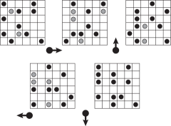
Figure 1: An illustration of the one cycle of the model. Black circles mark unblocked particles that are free to move in the following move, while grey particles are blocked for the next move. The directions of the moves are indicated by arrows, and periodic boundary conditions are employed.

We typically “strobe” the system, comparing configurations before and after a full cycle. Thus, a particle which was not blocked at all during a cycle will appear to be stationary, since it returns to its initial configuration. Note that it is not necessarily the case that a particle which is blocked for one or more of the moves will fail to return to its original location. We will refer to particles or clusters of particles which return to their starting positions at the end of a cycle as ‘invariant under the dynamics’, or ‘stationary’. Figure 2 shows two such invariant patterns at half filling.

We have studied the behavior of the model through numerical simulations starting from random initial conditions for particle densities $\rho\in\left[0,0.5\right]$. We note that the model is self-dual: because of particle-hole symmetry, higher densities $\rho\in\left[0.5,1\right]$ are mapped onto the lower half-interval by $\rho\rightarrow(1-\rho)$. This can be seen easily at the level of a single move where the motion of a particle to the right can be envisioned as the motion of a vacancy to the left. Thus, the behavior at densities $\rho>0.5$ is identical to behavior at density $1-\rho$ if vacancies are tracked instead of particles.

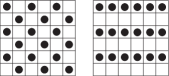
Figure 2: Two invariant configurations, checkerboard and striped, each at half filling. Each maps onto itself after one cycle.

The steady state behavior of the dynamics is very different from many other driven systems Corte et al. (2008); Lübeck (2004); Aldana et al. (2003) in that for the full range of density, the system self-organizes, displaying no chaotic behavior. At low densities this proceeeds in a trivial manner with almost all the particles becoming separated, allowing them to complete a cycle of the motion unhindered by any blocking, with but a few undergoing periodic motion with a short period. At these low densities, the rearrangements leading to the steady state are local in character, as might be expected. At higher densities, however, the organization to a steady state occurs on long length scales. This is seen both in the long relaxation dynamics and in the characteristic formation of large, well-defined regions.

These regions are invariant under the dynamics, and appear static under strobing. They always self-organize into three possible patterns: either vertical stripes, horizontal stripes or a checkerboard pattern (see Figure 2), with occasional point defects. In fact, the whole steady-state configuration can be viewed as a mosaic of grains of these patterns as shown in Figure 3. We emphasize that all three of these patterns have a density of $\rho=0.5$, and that each of them is stable against the removal or addition of a particle in the bulk (these two operations are the same due to the particle-hole symmetry). This differs considerably from directed percolation models which also have invariant configurationsCorte et al. (2008), but which are not stable to local perturbations.

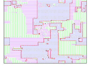
Figure 3: An example of steady state configuration at $\rho=0.5$. Blue marks the checkered pattern, green marks the vertical striped pattern and pink marks the horizontal striped pattern. The paths of mobile particles are indicated in red.

It is clear from the above that stationary configurations at many densities exist, being easily obtained by adding (or removing) particles in the bulk of the different grains. For example, any number of particles can be added to the checkered pattern at any location and the configuration will still be stationary. It is therefore surprising that in a broad range of densities centered around $\rho=0.5$ the system arranges itself into a mosaic of grains of almost perfectly ordered striped or checkerboard patterns at half filling. These form as a result of a dynamical process which we discuss presently.

Not all the particles in the steady-state are stationary; a small fraction of “frustrated” particles move about the system. Remarkably, these particles are confined to one dimensional directed closed paths which intersect neither themselves nor other paths, although they often form very complicated winding curves, especially near $\phi=0.5$; this is depicted in Figure 3. These particles move in periodic orbits along their designated paths, with periods which may be extremely long.

As seen in Figure 3, there is a close relation between the invariant grains and the paths of the moving particles, with the paths appearing on boundaries separating checkerboard and striped patterns. The motion along each path is unidirectional and occurs either clockwise or counter-clockwise depending on the pattern in the interior of the path. If the checkered region is in the interior, the motion is clockwise, while when the internal region is striped, the motion is counter-clockwise. The latter case is rare. It is not the case that motion occurs on every boundary between checkered and striped phases; in these cases, the boundary is filled with vacancies ($\rho<0.5$) or completely occupied ($\rho>0.5$).

To see how the motion on the stripe-checkerboard grain boundary occurs we track two particles explicitly in Figure 4. Note that the motion (for example, vertical jumps of two lattice spacings, as in the figure) cannot be attributed to a single tagged particle hopping along the path, but rather through the motion of two particles. For this reason the paths in figure 3 appear as dashed lines.

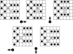
Figure 4: Motion of tagged particles at a stripe-checkerboard boundary. Comparing the state at the end of a cycle with that at the beginning (and regarding the particles as indistinguishable), gives the illusion of a single particle being displaced downward by two units. This is, of course, not possible for a single particle acting alone.

The dynamical mechanism responsible for the almost perfect ordering of the checkerboard and striped patterns is collective in nature, and occurs in the latter stages of the transient period, when paths have formed but are not quite stable. In this stage, in addition to the motion which occurs along paths as in the steady-state, the motion sometimes penetrates into the grain bulk as a front “sweeping” across the grain. In the wake of such a moving front, the nature of the pattern changes, from striped to checkerboard or vice versa (see supplemental material), and new paths are formed. In this coarsening process the size of the clusters grows until the steady state is reached and the paths are stable.

We begin our quantitative analysis of the steady-state by examining the paths. These are mapped out numerically by allowing the system to reach steady-state, and then time-averaging over the moving particles. In particular, we calculate $\rho_{ij}\equiv\left\langle\left|X_{ij}\left(t+1\right)-X_{ij}\left(t\right)\right|\right\rangle$, where $X_{ij}\left(t\right)\in\left[0,1\right]$ marks the occupancy of the site with coordinates $\left(i,j\right)$ at time $t$, with $t+1$ being reckoned at the end of the following cycle. In the invariant regions, $\rho_{ij}=0$, while along a path, $\rho_{ij}$ is non-zero, and its value is related to the density of particles along the path. It is worth noting that the value of $\rho_{ij}$ is constant along a path, so that the flux along any given path is constant. An example the non-zero elements of $\rho_{ij}$ is presented in Figure 5.

In some instances, two paths touch each other, raising the question of whether to consider these as independent paths or a single path with a loop. We argue in favor of the former interpretation for the following reasons. First, particles traversing touching portions move in opposite directions, and second, the flux of moving particles is constant on all points of a given path and typically different from other paths. There are rare exceptions where two touching paths “interact”, with a particle jumping between the two paths. In this case, in the touching region $\rho_{ij}$ has a value different from that of both parent paths where there is no touching. This leads us to define a path as the set of connected points with the same $\rho_{ij}$. An alternative, not presented here, is to track the location of tagged particles and measure the paths they follow; this yields the same qualitative behavior.

As seen in Figure 5, paths are both non-intersecting and self-avoiding. There are several different ensembles of self-avoiding paths known, among them simple closed curves, self-avoiding random walks, and loop erased walksMajumdar (1992). These differ in their fractal dimension, which can be characterized by the scaling of the radius of gyration $R_{g}=\sqrt{\left\langle\left|\vec{r}-\vec{r}_{0}\right|^{2}\right\rangle}$, where $\vec{r}_{0}$ is the center of mass of the walk. The gyration radius scales as a power of the path length $\ell$, namely, $R_{g}\sim\ell^{\nu}$, where for a regular polygon $\nu=1$, for a self-avoiding walk $\nu=0.75$Duplantier and Saleur (1987) and for loop erased walk $\nu=0.8$Majumdar (1992). In Figure 6 we show $R_{g}^{2}\left(\ell\right)$ at $\rho=0.5$. The behavior of $R_{g}\left(\ell\right)$ is consistent with a power-law with $\nu=0.75$ or $\nu=0.8$, though some deviation occurs for large $\ell$. This deviation may result from finite size effects such as the boundary which limits the gyration radius, while another possibility is that it is due to the interaction between the different paths, causing crowding. An estimate to the order of magnitude of the linear size of the cluster at which the crossover occurs can be estimated from where $R_{g}\left(\ell\right)$ deviates from a power-law; this appears to be of order of several hundred.

In addition to $R_{g}$, we measured $P\left(\ell\right)$, the distribution of paths of length $\ell$, for different densities. At low densities, the fall-off of $P\left(\ell\right)$ at short distances is consistent with exponential decay. At $\rho\gtrsim 0.475$, the decay appears to be power-law: $P\left(\ell\right)\propto\ell^{-\gamma}$ , where $\gamma\simeq 1.75$, as seen in Figure 7. This power-law behavior persists up to a system size-dependent length, at which the distribution falls off more quickly. As shown in Figure 8 there is little difference between $L=800$ and $L=1600$ at $\rho=0.5$ with similar behavior at other densities. Our results are inconclusive as to whether this dropoff is due to finite size effects or to a finite correlation length, and as such it is difficult to conclude with confidence whether or not the system becomes critical in the limit of $L\rightarrow\infty$, or whether a phase transition occurs or is avoided.

The value of $\gamma$ is consistent with the probability of occurrence of a path being inversely proportional to its area: The linear size of a path scales as $R_{g}$, and if the frequency of occurrence is inversely proportional to area, the probability density goes as $P\left(R_{g}\right)\propto R_{g}^{-2}$. Since $R_{g}\propto\ell^{\nu}$, it follows that $P\left(\ell\right)\propto\ell^{-\nu-1}$, so the exponents are related by $\gamma=1+\nu$. For self avoiding random walks, $\nu=0.75$, giving $\gamma=1.75$, which is consistent with our measurements.

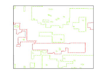
Figure 5: An example of the paths traced out by moving particles in the steady state, with $L=400$ and $\rho=0.5$. The red trajectory marks the longest path. Note that the dotted nature of the paths is due to the motion of a pair, as shown in Figure 4.

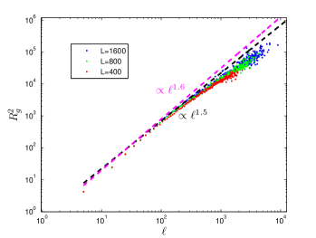
Figure 6: Squared radius of gyration as a function of the path length for different system sizes at $\rho=0.5$. Possible scaling relations $\ell^{2\nu}$ with $\nu=0.75$ and $0.8$ are presented.

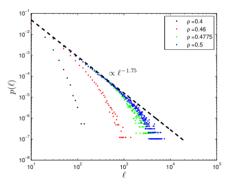
Figure 7: The distribution of path lengths for different densities, here $L=1600$. The black line is $\ell^{-1.75}$.

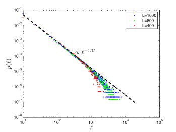
Figure 8: The distribution of path lengths at $\rho=0.5$ for different system sizes. The black line is $\ell^{-1.75}$.

To gain insight into the dynamics, we measure the density of moving particles as a function of time, which in analogy to the directed percolation transitions, we call the active density, denoted $\rho_{a}\left(t\right)$. For low densities, $\rho_{a}\left(t\right)$ decays to its asymptotic value $\rho_{a}\left(t=\infty\right)$ in an exponential fashion. This asymptotic value is shown in Figure 9 as a function of the density, and shows a steep rise at $\rho\simeq 0.475$. As the density grows, the time scale on which $\rho_{a}\left(t\right)$ decays grows, perhaps even diverging.

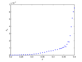
Figure 9: The asymptotic density of mobile particles $\rho_{a}\left(t=\infty\right)$ in the steady state for a system of size $L=1000$.

While it is tempting to conclude that there may be a phase transition in the vicinity of $\rho=0.5$, our results on this point are not conclusive. While the power-law distribution and the long time scales suggests a nearby critical point, it is not certain the system in thermodynamic limit indeed reaches this point.

We thank Alexander Grosberg and Paul Chaikin for interesting and useful discussions. DL acknowledges support from Israel Science Foundation grant 1254/12 and US - Israel Binational Science Foundation grant 2008483. DH thanks the US - Israel Binational Science Foundation for an R. Rahamimoff Travel Grant. We would like to thank the Center for Soft Matter Research at NYU and the Initiative for Theoretical Science of the Graduate Center of CUNY for their hospitality while this work was being conducted.

References

- Melo et al. (1995) F. Melo, P. B. Umbanhowar, and H. L. Swinney, Phys. Rev. Lett. 75, 3838 (1995).
- Tang et al. (1987) C. Tang, K. Wiesenfeld, P. Bak, S. Coppersmith, and P. Littlewood, Phys. Rev. Lett. 58, 1161 (1987).
- Biham et al. (1992) O. Biham, A. A. Middleton, and D. Levine, Phys. Rev. A 46, R6124 (1992).
- Corte et al. (2008) L. Corte, P. M. Chaikin, J. P. Gollub, and D. J. Pine, Nature Physics 4, 420 (2008).
- Aldana et al. (2003) M. Aldana, S. Coppersmith, and L. P. Kadanoff, in Perspectives and Problems in Nolinear Science, edited by E. Kaplan, J. E. Marsden, and K. R. Sreenivasan (Springer New York, 2003), pp. 23–89.
- (6) J. R. Royer and P. M. Chaikin, private communication.
- Lübeck (2004) S. Lübeck, Int. J. Mod. Phys. B 18, 3977 (2004).
- Majumdar (1992) S. N. Majumdar, Phys. Rev. Lett. 68, 2329 (1992).
- Duplantier and Saleur (1987) B. Duplantier and H. Saleur, Nuclear Physics B 290, 291 (1987).