Exploration vs Exploitation vs Safety:
Risk-Aware Multi-Armed Bandits

Abstract

Motivated by applications in energy management, this paper presents the Multi-Armed Risk-Aware Bandit (MaRaB) algorithm. With the goal of limiting the exploration of risky arms, MaRaB takes as arm quality its conditional value at risk. When the user-supplied risk level goes to 0, the arm quality tends toward the essential infimum of the arm distribution density, and MaRaB tends toward the MIN multi-armed bandit algorithm, aimed at the arm with maximal minimal value. As a first contribution, this paper presents a theoretical analysis of the MIN algorithm under mild assumptions, establishing its robustness comparatively to UCB. The analysis is supported by extensive experimental validation of MIN and MaRaB compared to UCB and state-of-art risk-aware MAB algorithms on artificial and real-world problems.

1 Introduction

The multi-armed bandit (MAB) framework has been intensively investigated in the last decade, handling the exploration vs exploitation dilemma through diverse selection rules, e.g. the upper confidence bound (UCB) criterion (Auer et al., 2002), KL-UCB (Maillard et al., 2011) or Thompson sampling (Chapelle and Li, 2011). The rise of MAB studies is explained as they tackle the rigorous analysis of algorithms in a both simplified and challenging setting. On the one hand, the MAB framework defines a simplified reinforcement learning problem (Sutton and Barto, 1998; Szepesvari, 2010), where the state space involves a single state. On the other hand, MAB is concerned with lifelong learning, and the optimization of the policy return while learning it. RL classically distinguishes the learning phase, and the production phase where the learned policy is applied. Most generally MAB makes no such distinction and aims at minimizing the cumulative regret suffered compared to the oracle strategy, during the whole learning/production life of the MAB system.

This paper specifically focuses on application domains where the exploration of the environment involves hazards and risks. Examples of such domains are energy management and robotics. In robotics, policies learned using a generative model of the environment (e.g. a simulator) happen to be inaccurate when ported on the actual robot, a phenomenon known as reality gap. On the other hand, training the robot in-situ entails significant risks due to mechanical fatigue and hazards. In the domain of energy management, simulators define noisy optimization problems as they must reflect the large variance of the energy load, demand and price along time; in the meanwhile, exploratory policies face huge losses if insufficient supply must be compensated for by buying additional energy.

In risky environments, the goal becomes to learn a policy which achieves some trade-off between exploration, exploitation and safety: while the goal is to minimize the regret through a standard exploration vs exploitation trade-off, one also wants to minimize the risk incurred by the learned policy and/or to maximize the safety of the learning agent. Risk minimization is also enforced by considering short time horizons.

The importance of risk minimization, either within the MAB setting (Sani et al., 2012; Maillard, 2013) or generally in reinforcement learning (Moldovan and Abbeel, 2012b) has been recently acknowledged (section 2). A new algorithm, the multi-armed risk-aware bandit (MaRaB) algorithm, is presented in section 3. MaRaB aims at the arm with maximal conditional value at risk level $\alpha$ (CVaR_α), where CVaR_α is the expected policy return in the prescribed quantile. When $\alpha$ goes to 0, MaRaB tends toward the MIN multi-armed bandit algorithm, aimed at the arm with maximal minimal value. A theoretical analysis of the MIN algorithm shows that it achieves logarithmic regret under mild assumptions (section 4). Extensive empirical validation on artificial problems shows that MaRaB less explores the arms with low distribution tails compared to UCB and (Sani et al., 2012), at the expense of a moderate regret increase compared to UCB. A real-world problem related to battery management with a stochastic demand is also considered to investigate the robustness of the approach (section 5). The paper concludes with a discussion and some perspectives for further research.

2 State of the art

After introducing the multi-armed bandit (MAB) formal background and referring the reader to (Robbins, 1952; Auer et al., 2002) for a comprehensive presentation, this section briefly reviews the state of the art related to risk-aware MAB strategies.

2.1 Formal background

A multi-armed bandit problem involves $K$ independent arms, each of which has an unknown reward distribution with bounded discrete or continuous support. The literature mostly considers two settings, that of Bernoulli distributions where the $i$-th arm yields reward 1 with probability $\mu_{i}$ and reward 0 otherwise, and that of distributions with support $[0,1]$, with mean $\mu_{i}$ and standard deviation $\sigma_{i}$. Let $T$ denote the time horizon. At each time step $t=1\ldots T$, a MAB algorithm selects an arm $i_{t}$ and receives reward $r_{i_{t},n_{i,t}}$, drawn after the $i_{t}$-th distribution, where $n_{i,t}$ denotes the number of times the $i$-th arm has been selected up to time $t$. The choice is made upon the basis of the empirical estimates of the $K$ arm distributions so far, the empirical mean estimate $\widehat{\mu_{i,t}}$ ($\widehat{\mu_{i,t}}=\frac{1}{n_{i,t}}\sum_{u=1}^{u=n_{i,t}}r_{i,u}$) and possibly the empirical variance estimate $\widehat{\sigma_{i,t}}$ (${\widehat{\sigma_{i,t}}}^{2}=\frac{1}{n_{i,t}}\sum_{u=1}^{u=n_{i,t}}(r_{i,u}-\widehat{\mu_{i,u}})^{2}$). The MAB goal is to maximize the sum of gathered rewards along learning, or equivalently to minimize the cumulative regret suffered compared to the oracle strategy, which plays the best arm $i^{*}$ in each time step. One distinguishes the theoretical cumulative regret at time $t$, denoted $\mathcal{R}_{t}$, and the empirical cumulative regret, denoted $\widehat{\mathcal{R}_{t}}$, respectively defined as:

$$\mathcal{R}_{t}=t\times\mu_{i^{*}}-\sum_{k=1}^{K}n_{k,t}\mu_{k}\hskip 72.26999pt\widehat{\mathcal{R}_{t}}=t\times\mu_{i^{*}}-\sum_{k=1}^{K}n_{k,t}\widehat{\mu_{k,t}}$$

We will use the theoretical cumulative regret in the algorithm analysis (section 4). Theoretical or empirical cumulative regrets will be used to experimentally assess the algorithms performance (section 5), granted that the difference $|\mathcal{R}_{t}-\widehat{\mathcal{R}_{t}}|$ is in $O(\log(t))$ (Coquelin and Munos, 2007).

Regret minimization is known to be an exploitation vs exploration trade-off problem: the best empirical arm should be selected often to maximize the actual gathered reward (exploitation); but some exploration is also required to actually identify the best arm. Two prominent MAB strategies are the $\epsilon$-greedy strategy, which selects the best empirical arm with probability $1-\epsilon$ and uniformly selects another arm with probability $\epsilon$, and the celebrated upper confidence bound (UCB) strategy proposed by Auer et al. (2002), which selects at time $t$ the arm maximizing criterion $\widehat{\mu_{i,t}}+C\sqrt{\frac{log(t)}{n_{i,t}}}$, with $C>0$ a parameter controlling the exploration vs exploitation tradeoff. Another strategy is the KL-UCB strategy (Maillard et al., 2011). While the $\epsilon$-greedy strategy suffers a linear regret, UCB and KL-UCB suffer a logarithmic regret, which is known to be optimal (Lai and Robbins, 1985). KL-UCB further improves on UCB as it yields the optimal regret rate.

2.2 Related work

An emerging trend in the field of reinforcement learning and MAB is concerned with the risk issue, when the exploring agent might face hazards going beyond mere under-optimal performances. In such cases, mottos such as Optimism in front of the Unknown! attached to the UCB strategy, are inappropriate. A first issue concerns the definition of risks. Several definitions have been proposed to account for risk awareness and risk aversion, taking inspiration from the literature in economics (Arrow, 1971).

The first criterion referred to as mean-variance (MV) (Markowitz, 1952) considers a weighted sum of the reward expectation $\mu$ of the policy and its estimated standard deviation. Formally, the goal is to find a policy minimizing $\sigma^{2}-\rho\mu$, where $\rho>0$ increases like the user’s risk tolerance.

The conditional value at risk (CVaR) considers the quantiles of the reward distribution. Formally, let $0<\alpha<1$ be the target quantile level. The associated quantile value $v_{\alpha}$ is defined if it exists as the maximal value such that $X$ is less than $v_{\alpha}$ with probability $\alpha$ ($Pr(X<v_{\alpha})=\alpha$, with $X$ the reward random variable). The remainder of the paper only considers continuous distributions, where $v_{\alpha}$ is always defined; the conditional value at risk $\alpha$ noted $\mbox{CVaR}_{\alpha}$ is then defined as the average reward conditionally to $X<v_{\alpha}$: $\mbox{CVaR}_{\alpha}[X]={\rm IE}[X|X<v_{\alpha}]$. Note that when the quantile level $\alpha$ goes to 0, CVaR_α maximization coincides with the standard max-min strategy, aimed at the arm with maximal minimum reward. CVaR maximization thus defines a relaxation of the max-min strategy, with quantile level $\alpha$ as relaxation parameter.

Another criterion, the rank dependent utility (Quiggin, 1993) inspired from the prospect theory due to Tversky and Kahneman (1979), is meant to model the distorted perception of probabilities, e.g. the over-estimation of rare events, through weighting the event rewards with a (non-linear) function of their rank. The RDU criterion will not be considered further as it relies on a complex specification of the risk aversion, whereas the above MV and CVaR criteria involve a single scalar parameter, respectively $\rho$ and $\alpha$.

Risk aversion has been considered in the MAB setting, only tackling the mean-variance criterion to our best knowledge (Sani et al., 2012). Two algorithms are proposed. The first one, referred to as MV-LCB, aims at minimizing the MV cumulative regret. It proceeds by adapting the UCB approach in the finite horizon $T$ context, selecting in each step $t$ the arm maximizing $\widehat{\sigma_{i,t}}^{2}-\rho\widehat{\mu_{i,t}}-(5+\rho)\sqrt{\frac{log(\frac{1}{\delta})}{2n_{i,t}}}$, where $\delta$ is adjusted depending on the time horizon $T$. As shown by Sani et al. (2012), this selection rule leads to upper-bounding the theoretical cumulative regret (related to the MV criterion) $R_{t}/t$ by $O(\frac{\log^{2}(t)}{t})$. A simpler strategy referred to as ExpExp decouples the exploration and the exploitation phases. All arms are uniformly launched during the exploration phase, and the arm with optimal empirical MV is selected ever after during the exploitation phase, with an $O(KT^{-\frac{1}{3}})$ regret bound if the length $\tau$ of the exploration phase is fixed to $K(\frac{T}{14})^{2/3}$.

Risk issues have also been considered in the neighbor field of reinforcement learning in the last years. A first strategy relies on reversibility constraints, i.e. only visiting states $s$ such that one can always get back from $s$ to the initial state (Moldovan and Abbeel, 2012a). In a further work, Moldovan and Abbeel (2012b) proceed by considering an exponential utility function, where the policy return $J$ is replaced by expression $exp\{J/\theta\}$. Parameter $\theta$ reflects the user’s risk tolerance, akin the $\rho$ parameter in the mean var setting, with the difference that $\rho$ is weighted by the empirical standard deviation of the rewards.

Another approach due to Mannor and Tsitsiklis (2011) formalizes risk-aware reinforcement learning as a multi-objective RL problem, aimed at simultaneously maximizing the cumulative reward and minimizing the cumulative standard deviation.

3 Overview of MaRaB

This section describes the Multi-Armed Risk-Aware Bandit (MaRaB) algorithm, with same notations as in section 2.1.

The arm quality is set to its conditional value at risk $\alpha$, where parameter $\alpha$ ($0<\alpha<1$) is set by the user. After Chen (2008), a non-parametric, consistent estimate of the conditional value at risk $\alpha$ of arm $i$, denoted $\widehat{CVaR_{\alpha,i}}$ (or $\widehat{CVaR_{i}}$ for notational simplicity), is given as the average of the $\alpha$ quantile of rewards $r_{i,u},u=1\ldots n_{i,t}$: assuming with no loss of generality that rewards are ordered by increasing value ($r_{i,u}\leq r_{i,u+1}$), and noting $n_{i,t,\alpha}$ the ceiling integer of $\alpha\cdot n_{i,t}$ ($\mbox{$n_{i,t,\alpha}$}=\lceil\alpha n_{i,t}\rceil$), then $\widehat{CVaR_{i}}$ is set to the average of the lowest $n_{i,t,\alpha}$ rewards:

$$\mbox{$\widehat{CVaR_{i}}$}=\frac{1}{\mbox{$n_{i,t,\alpha}$}}\sum_{u=1}^{\mbox{$n_{i,t,\alpha}$}}r_{i,u}$$ (1)

The goal of MaRaB is to find the arm with maximal $\widehat{CVaR_{i}}$. The selection rule controlling the exploration vs exploitation tradeoff proceeds by selecting the arm with best lower confidence bound on its CVaR:

$$\mbox{select $i_{t}$~{}}=\mbox{argmax}\left\{\mbox{$\widehat{CVaR_{i}}$}-C\sqrt{\frac{\log(\lceil t\alpha\rceil)}{\mbox{$n_{i,t,\alpha}$}}}\right\}$$ (2)

with $C>0$ a parameter controlling the exploration vs exploitation tradeoff.

MaRaB features a risk-averse or pessimistic behavior, due to the negative exploratory term in Eq. 2 : if two arms have same empirical CVaR, MaRaB will favor the arm which has been selected more often in the past. Note that such a behavior is actually observed in the economic realm, as trust $-$ i.e. a positive bias toward known good partners $-$ is at the core of economic exchanges. Such a bias indeed makes sense whenever exchanges with unknown partners involve risks.

A lack of exploration usually leads to myopic and under-optimal choices, sticking to the best options first encountered. Such a myopic behavior is however prevented in MaRaB for the following reason: MaRaB examines each arm along two phases. In the first phase, referred to as initial phase ($n_{i,t}<\frac{1}{\alpha}$), the empirical quality of the $i$-th arm is set to its minimum reward (Eq. 1), and therefore it monotonically decreases along time. In the second phase, referred to as stabilization phase, the estimate of the conditional value at risk is computed with increasing accuracy, with an approximation error going to 0 like $\sqrt{n_{i,t}}$ (Chen, 2008).

The duration of the initial phase increases as $\alpha$ decreases, as the maximization of the conditional value at risk $\alpha$ boils down to a standard max-min optimization problem. In the early iterations, the MaRaB behavior thus coincides with that of the MIN algorithm, selecting in each time step the arm with maximal minimum reward. The only difference comes from the negative exploration term (lower confidence bound, LCB). MaRaB thus actually achieves some exploration in the beginnings: the arm quality $\widehat{CVaR_{i}}$ monotonically decreases as the $i$-th arm is more visited ($n_{i,t}$ increases) in its initial phase, forcing MaRaB to consider less visited arms.

However, if an arm gets poor rewards the first times it is visited, there is little chance it is visited again, all the more so as better arms enter their second phases (and their empirical quality converges toward their true conditional value at risk): there is no positive exploration term guaranteeing that any arm will be visited infinitely many times as $t$ goes to infinity.

The theoretical analysis, presented in the next section, will thus focus on the limit algorithm of MaRaB, the MIN algorithm.

4 Analysis

This section presents the analysis of the MIN algorithm, selecting in each time step the arm with maximal empirical minimal value, as MIN is the limit algorithm of MaRaB when the risk level $\alpha$ goes to 0 and the exploratory constant $C$ is set to $0$.

Under the assumption that the best arm w.r.t. its essential infimum also is the best arm in terms of expectation, it is shown that MIN achieves same logarithmic regret as UCB, with similar rate. Under slightly stronger assumptions, the MIN regret rate is significantly lower than for UCB. These two results rely on two lemmas. Firstly, under mild assumptions, the empirical minimum value for every arm converges exponentially fast toward its essential infimum. Secondly, with high probability over all arms their empirical minimum value are exponentially close to their essential minimum, where the probability increases exponentially fast with the number of iterations.

Lemma 4.1

Let $\nu$ be a bounded distribution with support in $[0,1]$, with $a$ its essential infimum, and let us assume that $\nu$ is lower bounded in the neighborhood of $a$:

$$\exists A>0,\forall\epsilon>0,\mathbb{P}(X\leq a+\epsilon)\geq A\epsilon\mbox{~{} with $X$ r.v. $\sim\nu$}$$ (3)

Let $x_{1}\ldots x_{t}$ be a t-sample independently drawn after $\nu$. Then, the minimum value over $x_{u},u=1\ldots t$ goes exponentially fast to $a$:

$$\mathbb{P}(\underset{1\leq u\leq t}{\min}x_{u}\geq a+\epsilon)\leq\exp(-tA\epsilon)$$ (4)

Proof 4.1.

As the $x_{u}$ are iid, it comes:

$$\mathbb{P}(\underset{1\leq u\leq t}{\min}x_{u}\geq a+\epsilon) = \mathbb{P}(\forall u\in\{1,\ldots,t\},x_{u}\geq a+\epsilon)$$

$$= \prod_{u=1}^{t}\mathbb{P}(x_{u}\geq a+\epsilon)\leq(1-A\epsilon)^{t}\leq exp(-tA\epsilon)$$

where the last inequality follows from $(1-z)\leq exp(-z)$.

Under the assumption of a lower-bounded distribution probability in the neighborhood of its minimum, the convergence toward the minimum thus is faster than the convergence toward the mean. Specifically, the Hoeffding bound on the convergence toward the mean decreases exponentially like $-t\epsilon^{2}$, whereas after Eq. 4 the convergence toward the min decreases exponentially like $-tA\epsilon$.

Under the same assumptions, with high probability the empirical min of each arm is exponentially close to its essential infimum after each arm has been tried $t$ times.

Lemma 1.

Let $\nu_{1}\ldots\nu_{K}$ denote $K$ distributions with bounded support in $[0,1]$ with $a_{i}$ their essential infimum. Let us assume that $\nu_{i}$ is lower bounded by some constant $A$ in the neighborhood of $a_{i}$ for $i=1\ldots K$.
Denoting $x_{i,u}$, $~{}u=1\ldots t$, $i=1\ldots K$, $t$ samples independently drawn after $\nu_{i}$, one has:

$$\mathbb{P}(\exists i\in\{1,\ldots,K\},\underset{1\leq u\leq t}{\min}x_{i,u}\geq a_{i}+\epsilon)\leq K\exp(-tA\epsilon)$$ (5)

Proof 4.2.

After Lemma 4.1,

$$\mathbb{P}(\exists i\in\{1,\ldots,K\},\underset{1\leq u\leq t}{\min}x_{i,u}\geq a_{i}+\epsilon) \leq 1-(1-(1-A\epsilon)^{t})^{K}$$

$$\leq K(1-A\epsilon)^{t}$$

$$\leq K\exp(-tA\epsilon)$$

Where the first inequality follows from $(1-z)^{y}\geq 1-y.z$ and the second inequality from $(1-z)\leq exp(-z)$, which concludes the proof.

Under the above assumptions on the arm distributions, if the optimal arm in terms of min value also is the optimal arm in terms of mean value, then the MIN algorithm achieves a logarithmic regret.

Proposition 2.

Let $\nu_{1}\ldots\nu_{K}$ denote $K$ distributions with bounded support in $[0,1]$ with $\mu_{i}$ (resp. $a_{i}$) their mean (resp. their essential infimum). Let us further assume that $\nu_{i}$ is lower bounded by some constant $A$ in the neighborhood of $a_{i}$ for $i=1\ldots K$, and that the arm with best mean value $\mu^{*}$ also is the arm with best min value $a^{*}$. Let $\Delta_{\mu,i}=\mu^{*}-\mu_{i}$ (resp. $\Delta_{a,i}=a^{*}-a_{i}$) denote the mean-related (resp. essential infimum-related) margins. Then, with probability at least $1-\delta$, the cumulative regret is upper bounded as follows:

$${\mathcal{R}_{t}}\leq\frac{K-1}{A}\frac{\Delta_{\mu,\max}}{\Delta_{a,\min}}\log\left(\frac{tK}{\delta}\right)+(K-1)\Delta_{\mu,\max}$$ (6)

with $\Delta_{a,\min}=\underset{i}{\min}\,\Delta_{a,i}$ and $\Delta_{\mu,\max}=\underset{i}{\max}\,\Delta_{\mu,i}$.

Furthermore, the expectation of the cumulative regret is upper-bounded as follows for $t$ sufficiently large ($t\geq\frac{K-1}{A}\frac{\Delta_{a,\min}}{\Delta_{\mu,\max}}$):

$$\mathbb{E}[{\mathcal{R}_{t}}]\leq\frac{K-1}{A}\frac{\Delta_{\mu,\max}}{\Delta_{a,\min}}\left(\log\left(\frac{t^{2}KA}{K-1}\frac{\Delta_{a,\min}}{\Delta_{\mu,\max}}\right)+1\right)+(K-1)\Delta_{\mu,\max}$$ (7)

Proof 4.3.

Let us assume that there exists a single optimal arm (we shall return to this point below). Taking inspiration from Sani et al. (2012), let $x_{i,u}$ be independent samples drawn after $\nu_{i}$, and define the event set $\mathcal{E}$ as follows:

$$\mathcal{E}=\{\forall i\in\{1,\ldots,K\},\forall u\in\{1,\ldots,t\},\underset{1\leq s\leq u}{\min}x_{i,s}-a_{i}\leq\frac{\epsilon}{u}\}$$ (8)

The probability of the complementary set $\mathcal{E}^{c}$ is bounded after Lemma 1:

$$\mathbb{P}(\mathcal{E}^{c}) = \mathbb{P}(\exists i\in\{1,\ldots,K\},\exists u\in\{1,\ldots,t\},\underset{1\leq s\leq u}{\min}x_{i,s}-a_{i}>\frac{\epsilon}{u})$$

$$\leq \sum_{u=1}^{t}\mathbb{P}(\exists i\in\{1,\ldots,K\},\underset{1\leq s\leq u}{\min}x_{i,s}-a_{i}>\frac{\epsilon}{u})$$

$$\leq \min(1,tK\exp(-A\epsilon))$$

Let $t>1$ be an iteration where a sub-optimal arm $i$ is selected; this implies that the empirical min of the $i$-th arm is higher than that of the best arm $i^{*}$:

$$\underset{1\leq u\leq n_{i^{*},t-1}}{\min}x_{i^{*},u}<\underset{1\leq u\leq n_{i,t-1}}{\min}x_{i,u} \Leftrightarrow \underbrace{\underset{1\leq u\leq n_{i^{*},t-1}}{\min}x_{i^{*},u}-a_{i}}_{\geq a_{i^{*}}-a_{i}=\Delta_{a,i}}<\underbrace{\underset{1\leq u\leq n_{i,t-1}}{\min}x_{i,u}-a_{i}}_{\leq\frac{\epsilon}{n_{i,t-1}}(*)}$$

where $(*)$ holds if $t$ belongs to the event set $\cal E$, thus with probability at least $1-tKexp(-A\epsilon)$ after Lemma 1.
It follows that with probability at least $1-tKexp(-A\epsilon)$

$$\frac{\epsilon}{n_{i,t-1}}\geq\Delta_{a,i}\mbox{~{}hence~{}}n_{i,t}\leq\frac{\epsilon}{\Delta_{a,i}}+1$$

since $n_{i,t}\leq n_{i,t-1}+1$. With probability at least $1-tKexp(-A\epsilon)$, the cumulative regret ${\mathcal{R}_{t}}$ can thus be upper-bounded:

$${\mathcal{R}_{t}} = \sum_{i=1}^{K}n_{i,t}\Delta_{\mu,i}\leq\sum_{i=1}^{K}(\frac{\epsilon}{\Delta_{a,i}}+1)\Delta_{\mu,i}$$

$$\leq (K-1)\left(\frac{\Delta_{\mu,max}}{\Delta_{a,min}}\epsilon+\Delta_{\mu,\max}\right)\mbox{ with }\Delta_{\mu,\max}=\underset{1\leq i\leq K}{\max}\Delta_{\mu,i}\mbox{~{}and~{}}\Delta_{a,\min}=\underset{1\leq i\leq K}{\min}\Delta_{a,i}$$

Finally, by setting $\delta=\min(1,tK\exp(-A\epsilon))$, it follows that with probability $1-\delta$,

$${\mathcal{R}_{t}}\leq\frac{K-1}{A}\frac{\Delta_{\mu,max}}{\Delta_{a,min}}\log(\frac{tK}{\delta})+(K-1)\Delta_{\mu,\max}$$ (10)

In the case where there exists $k>1$ optimal arms, Eq. 10 still holds, by replacing $K-1$ factor with $K-k$.

The expectation of the cumulative regret is similarly upper-bounded:

$$\mathbb{E}[{\mathcal{R}_{t}}] = \mathbb{E}[\mathcal{R}_{t}\mathbb{I}_{\mathcal{E}}]+\mathbb{E}[\mathcal{R}_{t}\mathbb{I}_{\mathcal{E}^{c}}]$$

$$\leq \frac{K-1}{A}\frac{\Delta_{\mu,max}}{\Delta_{a,min}}\log(\frac{tK}{\delta})+(K-1)\Delta_{\mu,\max}+\delta t\mbox{ by bounding }{\mathcal{R}_{t}}\ \mbox{ by }t\mbox{ over }\mathcal{E}^{C}.$$

For $t$ sufficiently large ($t\geq\frac{K-1}{A}\frac{\Delta_{\mu,max}}{\Delta_{a,min}}$), by setting $\delta=\frac{K-1}{tA}\frac{\Delta_{\mu,max}}{\Delta_{a,min}}$, it comes :

$$\mathbb{E}[{\mathcal{R}_{t}}]\leq\frac{K-1}{A}\frac{\Delta_{\mu,max}}{\Delta_{a,min}}\left(\log\left(\frac{t^{2}KA}{(K-1)}\frac{\Delta_{a,\min}}{\Delta_{\mu,\max}}\right)+1\right)+(K-1)\Delta_{\mu,\max}$$ (11)

which concludes the proof.

Remark. UCB similarly achieves a logarithmic regret (Auer et al., 2002):

$$\mathbb{E}[\mathcal{R}_{t}]\leq 8\sum_{i\neq i^{*}}\frac{\log t}{\Delta_{\mu,i}}+(1+\frac{\pi^{2}}{3})\sum_{i=1}^{K}\Delta_{\mu,i}$$ (12)

where $i^{*}$ stands for the index of the optimal arm. MIN and UCB thus both achieve a logarithmic regret uniformly over $t$, where the regret rate involves the mean-related margin in UCB (resp. the min-related margin in MIN, multiplied by the lower-bound constant $A$ on the density in the neighborhood of the minimum).

A stronger result can be obtained for MIN, under an additional assumption on the lower tails of the arm distributions.

Proposition 3.

With same notations and assumptions as in Prop. 2, let us further assume that for every $i=1\ldots K,\Delta_{\mu,i}=\mu^{*}-\mu_{i}\leq a^{*}-a_{i}=\Delta_{a,i}$.

Then, with probability at least $1-\delta$,

$${\mathcal{R}_{t}}\leq\frac{K-1}{A}\log(\frac{tK}{\delta})+(K-1)\Delta_{\mu,\max}$$

with $\Delta_{\mu,\max}=\underset{i}{\max}\,\Delta_{\mu,i}$.

Furthermore, if $t>\frac{K-1}{A}$, the expectation of ${\mathcal{R}_{t}}$ is upper-bounded as follows :

$$\mathbb{E}[{\mathcal{R}_{t}}]\leq\frac{K-1}{A}\left(\log\left(\frac{t^{2}KA}{K-1}\right)+1\right)+(K-1)\Delta_{\mu,\max}$$ (13)

Proof 4.4.

The proof closely follows the one of Prop. 2, noting that in Eq. 4.3 $\Delta_{a,i}$ is now greater than $\Delta_{\mu,i}$. Setting $\delta=\frac{(K-1)}{tA}$ concludes the proof of Eq. 13.

Discussion. The comparison of Eq. 13 and Eq. 12 suggests that MIN might outperform UCB in the case where margins $\Delta_{\mu,i}$ are small, where distributions $\nu_{i}$ are not too thin in the neighborhood of the essential infimum (that is, $A$ is not too small), and the assumption $\Delta_{a,i}\geq\Delta_{\mu,i}$ holds.
Note that the latter assumption boils down to considering that better arms (in the sense of their mean) also have a narrower support for their lower tail, thus a lower risk. If this assumption does not hold however, then risk minimization and regret minimization are likely to be conflicting objectives.

A last remark is that the assumptions done (lower bounded distribution density in the neighborhood of the essential minimum and mean-related margin greater than the minimum-related margin) yield a significant improvement compared to the continuous distribution-free case, where the optimal regret is known to be $O(\sqrt{t})$ (Audibert and Bubeck, 2009, 2010).

5 Experimental validation

As proof of concept, UCB, MIN and MaRaB are first compared on favorable cases, using a problem generator satisfying the assumptions done in Prop 3. A general empirical validation follows, assessing MIN and MaRaB comparatively to UCB and to the risk-aware MV-LCB and ExpExp algorithms (Sani et al., 2012). Artificial problem instances are generated using a relaxed problem generator, which only satisfies the assumption of lower-bounded densities in the neighborhood of their minimum (section 5.2). A simplified real-world problem in the target application domain of energy management is also considered (section 5.3). The goal of experiments is to answer three questions. The first one is the price to pay in terms of performance loss for a risk-aware behavior, and how the cumulative regret increases with the number of iterations, specifically focussing on short time horizons (unless explicitly specified, the empirical cumulative regret is considered). The second question regards the robustness of the algorithms, and their sensitivity w.r.t. parameters. A third question is whether MaRaB, MV-LCB and ExpExp do avoid exploring risky arms; this question is investigated by inspecting the low tail of the gathered rewards.

The number $K$ of arms is set to 20. The time horizon is set to $T=K\times 100$ and $T=K\times 200$. For all problems, all results over (respectively the average result out of) 40 runs are displayed.

5.1 Proof of concept

An ad-hoc problem generator satisfying the assumptions done in Prop. 3 is used to compare MIN, UCB and MaRaB in the favorable case.

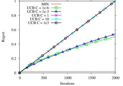
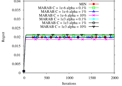
(a) MIN and UCB	(b) MIN and MaRaB
$C=10^{i},~{}i=-6\ldots 3$	$C=10^{i},~{}i=-6\ldots 3$, $\alpha=.1\%,1\%,10\%$)

Figure 1: Theoretical cumulative regret of UCB, MIN and MaRaB under the assumptions of Prop. 3, averaged out of 40 runs. Parameter $C$ ranges in $\{10^{i},i=-6\ldots 3\}$. Risk quantile level $\alpha$ ranges from .1% to 10%.
Left: UCB regret increases logarithmically with the number of iterations for well-tuned $C$; MIN identifies the best arm after 50 iterations and its regret is constant thereafter. Right: zoom on the lower region of Left, with MIN and MaRaB regrets; MaRaB regret is close to that of MIN, irrespective of the $C$ and $\alpha$ values in the considered ranges.

Each problem involves 20 arms. The $i$-th arm distribution $\nu_{i}$ is set to a uniform distribution on a segment in $[0,1]$, centered on $\mu_{i}$ with radius $r_{i}$ ($\nu_{i}=\mathcal{U}([\mu_{i}-r_{i},\mu_{i}+r_{i}])$). Mean $\mu_{i}$ (respectively radius $r_{i}$) decreases (resp. increases ) with $i$. The mean-related and minimum-related margins are respectively controlled from two generative parameters. The theoretical cumulative regrets of UCB, MIN and MaRaB are displayed in Fig. 1 (averaged out of 40 independent runs with $\mu^{*}=0.5,a^{*}=\mu^{*}-10^{-3}$ and maximal radius $0.5$). Parameter $C$ of UCB and MaRaB ranges in $\{10^{i},i=-6\ldots 3\}$ and the risk level $\alpha$ ranges from .1% to 10%. By construction, this artificial problem favors MIN against UCB; firstly it satisfies the assumptions of Prop. 3; moreover since distributions $\nu_{i}$ are uniform, $A\geq 1$. In this easy setting, MIN catches the best arm after 50 iterations and yields a constant regret thereafter (no exploration). MaRaB features the same behavior for a wide range of values of $C$ and $\alpha$; its very low sensitivity w.r.t. $C$ slightly increases for high values of $\alpha$ ($\alpha>20\%$). The disappointing UCB performance is blamed on the high variance of the worse arms, slowing down the accurate estimation of their mean.

5.2 Artificial problems

A second problem generator is considered, which only satisfies the assumption of a lower-bounded density in the neighborhood of the minimum (Eq. 3). Specifically, each problem involves 20 arms. The $i$-th arm distribution $\nu_{i}$ is set to a mixture of truncated Gaussians: i) its minimum $a_{i}$ is uniformly drawn in $[0,.05]$; ii) $n_{i}$ Gaussians are defined where $n_{i}$ is uniformly drawn in $1\ldots 4$; for $j=1\ldots n_{i}$ the $j$-th Gaussian ${\cal N}(\mu_{i,j},\sigma_{i,j})$, is defined by uniformly sampling $\mu_{i,j}$ in $[0,1]$ and $\sigma_{i,j}$ in $[.12,.5]$; furthermore, the $j$-th Gaussian is associated a probability $p_{i,j}$ such that $\sum_{j}p_{i,j}=1$. Upon selecting the $i$-th arm, the reward is drawn by: i) selecting the $j$-th Gaussian with probability $p_{i,j}$; ii) drawing a reward $r$ from ${\cal N}(\mu_{i,j},\sigma_{i,j})$; iii) going to i) if $r$ is not in the $[a_{i},1]$ interval (rejection-based truncation).

5.2.1 Cumulative regrets

The empirical cumulative regrets of UCB, MaRaB, MV-LCB and ExpExp are displayed in Fig. 2, reporting the empirical cdf of the regrets over 1,000 problem instances for short time (Fig. 2.(a)) and medium time (Fig. 2.(b)) horizons. All algorithm parameters are set to their best value after preliminary experiments. UCB yields the best cumulative regret overall whenever $C$ is well tuned. MaRaB suffers an extra regret compared to UCB; this extra regret is bounded in the considered experimental setting, and it seemingly does not increase as the time horizon increases. As could have been expected this extra regret decreases as $\alpha$ increases and the selection rule involves a better estimation of the empirical means. Interestingly, MaRaB shows a very low sensitivity w.r.t. $C$.

MV-LCB yields the worst regret of all strategies, with a very low sensitivity w.r.t. parameter $\rho$ on the considered problems. ExpExp significantly improves on MV-LCB with probability circa 90%; it even improves on UCB with probability 10% (circa 20% for medium time horizon). ExpExp yields very good results; the fact that it does never get very low cumulative regret is explained from its initial exploratory phase; a caveat is that its optimal setting used in the experiments requires the time horizon to be known in advance. MaRaB improves on ExpExp with probability 70%, albeit with maximal cumulative regrets (over the problem instances) higher than for ExpExp.

Overall, MaRaB with risk level $\alpha=20\%$ and untuned $C$ value yields results slightly less than UCB with tuned $C$, for both short and medium time horizons. The risk-aware MaRaB suffers a low regret increase compared to risk-neutral UCB, with a very low sensitivity w.r.t. $C$. Interestingly, a twice longer time horizon does not modify the performance order of the algorithms.

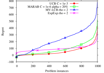
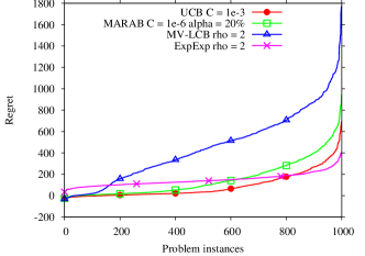
(a) Time horizon 2,000	(b) Time horizon 4,000

Figure 2: Empirical cumulative regret of UCB, MaRaB, MV-LCB and ExpExp on 1,000 problem instances (independently sorted for each algorithm) over short and medium time horizons. All algorithms are used with tuned parameters ($C=10^{-3},\alpha=20\%,\rho=2,\delta=\frac{1}{T^{2}},\tau=K(\frac{T}{14})^{2/3}$).

5.2.2 Risk Awareness

The effective risk avoidance of UCB, MV-LCB, ExpExp and MaRaB are investigated by inspecting the empirical cdf of the instant rewards on two representative artificial problems, with respectively low (Fig. 3, left) and high (Fig. 3, right) variance of the best arm.

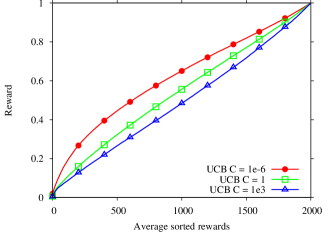
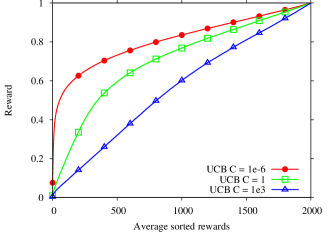
UCB with $C=10^{i},i=-6,0,3$
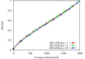
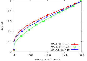
MV-LCB with $\rho\in\{1,2,10\},\delta=\frac{1}{T^{2}}$
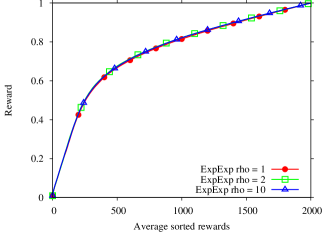
ExpExp with $\rho\in\{1,2,10\},\tau=K(\frac{T}{14})^{2/3}$
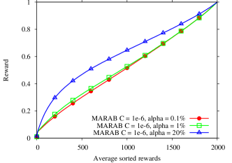
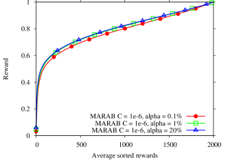
MaRaB with $C=10^{-6},\alpha\in\{0.1\%,1\%,20\%\}$

Figure 3: Comparative risk avoidance of UCB, MV-LCB, ExpExp and MaRaB on two representative artificial problems with low (left) and high (right) variance of the optimal arm. For each algorithm instant rewards averaged out of 40 runs are sorted. The time horizon is set to $T=2,000$.

The low tail of the cdf (worst average rewards gathered by the algorithm) indicates whether the algorithm actually tried poor arms. Fig. 3 confirms previous results: The noted sensitivity of UCB w.r.t. parameter $C$ unsurprisingly increases with the variance of the best arm (Fig. 3, top row). The bad performance of MV-LCB is confirmed; its sensitivity w.r.t. $\rho$ is low on the low variance problem as expected (Fig. 3, second row, left); its sensitivity w.r.t. $\rho$ is much higher on the high variance problem (Fig. 3, second row, right), with a best performance for medium values of $\rho$. ExpExp features an excellent risk avoidance as the risky trials only take place during the exploratory phase (Fig. 3, third row). The general robustness of MaRaB w.r.t. $C$ is confirmed; moreover, its robustness w.r.t. the risk level $\alpha$ on high variance problems is empirically shown (Fig. 3, bottom row). It is seen that for low to medium risk ($\alpha<20\%$), the quantile values $v_{\alpha}$ (section 2.2) are consistently higher for MaRaB than for ExpExp, which is explained again from the systematic exploratory phase in ExpExp.

5.3 Optimal energy management

The real-world problem motivating the presented approach is a battery management problem, where the environment is described by the energy demand and the energy cost in each time step. The decision to be taken in each time step is a real-value $x$, determining how much energy is either used from the battery (if $x>0$) or stored in the battery (if $x<0$). In each time step, one must meet the demand by buying $\min(0,\mbox{demand}-x)$ energy; the instant reward is the cost of the bought energy if the demand exceeds the available energy. Additionally, the battery loses some energy in each time step. A simplified setting is considered, where i) the energy cost is constant, the random process only dictates the energy demand in each time step; ii) 20 arms, corresponding to pre-defined strategies are considered. The strategy reward is drawn by uniform sampling with replacement from the 117 available realizations of the strategy.

Same general trends as for the artificial problems are observed on this real-world problem (Fig. 4): i) The cumulative regret is minimal for UCB with optimally tuned $C$; ii) MV-LCB is dominated by all other algorithms w.r.t. both risk avoidance and cumulative regret; iii) the ExpExp regret increases linearly during the exploration phase and then reaches a plateau; iv) MaRaB shows its good risk-avoidance ability regardless of the $C$ value, and MIN yields same results. Overall, MaRaB suffers a slight regret increase compared to UCB at its best, with a slightly better reward cdf in the region of low rewards.

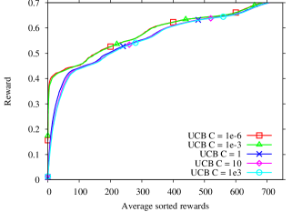
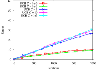
UCB. $C\in\{10^{-6},10^{-3},1,10,10^{3}\}$
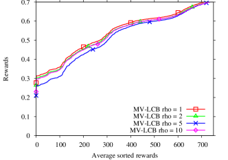
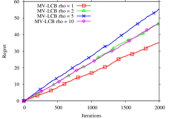
MV-LCB $\rho\in\{1,2,5,10\},\delta=\frac{1}{T^{2}}$
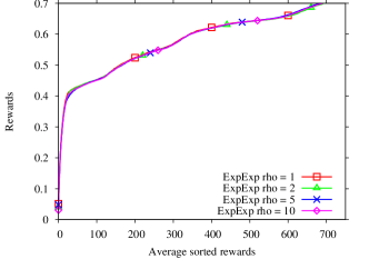
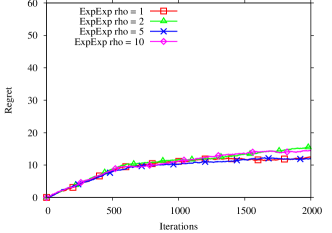
ExpExp $\rho\in\{1,2,5,10\},\tau=K(\frac{T}{14})^{2/3}$
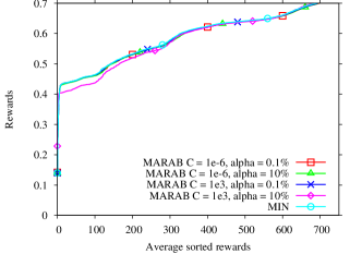
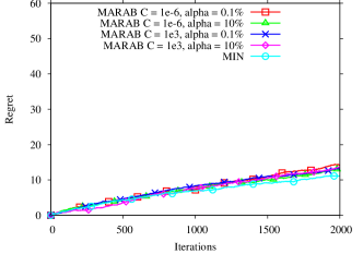
MaRaB $C\in\{10^{-6},10^{3}\},\alpha\in\{0.1\%,10\%\}$

Figure 4: Comparative performance of UCB, MV-LCB, ExpExpand MaRaB on a real-world energy management problem. Left: sorted instant rewards (truncated to the 37.5% worst cases for readability). Right: empirical cumulative regret with time horizon $T=100K$, averaged out of 40 runs.

6 Discussion and perspectives

The first contribution of the paper, as a step toward an effective trade-off between exploitation, exploration and safety, is to show the theoretical soundness of the MIN algorithm. This result relies on two main assumptions: i) same arms are optimal in the perspective of regret and risk minimization; ii) the arm reward distributions are lower bounded in the neighborhood of their minimum on the other hand. Not only does MIN achieve logarithmic regret; it also yields a better rate than UCB under the additional assumption that min-related margins are higher than mean-related margins. A second contribution is the MaRaB strategy, yielding a reduced risk at the expense of a moderate regret increase compared to UCB for short and medium time horizons, on artifial problems (which only satisfies the lower-bounded distribution assumption) and on a real-world one.

Further work is concerned with the analysis of MaRaB behavior, specifically its mean-related regret (under the assumption that the arm with best mean also is the arm with best CVaR) and its CVaR-related regret; another priority is to compare MaRaB behavior with that of Maillard (2013). A second perspective regards the case where the arms belong to a metric space; the goal becomes to exploit this metrix to enforce exploration safety. Last but not least, MaRaB will be extended to tree-structured search spaces to achieve e.g. safe sequential decision making.

We are grateful to J.-J. Christophe, J. Decock and the members of the Ilab Metis and Artelys, for fruitful collaboration. We thank the anonymous referees for their insightful comments.

References

- Arrow (1971) K.J. Arrow. Essays in the Theory of Risk-Bearing, chapter The Theory of Risk Aversion, pages 90–120. Markham, 1971.
- Audibert and Bubeck (2009) Jean-Yves Audibert and Sébastien Bubeck. Minimax policies for adversarial and stochastic bandits. In Proceedings of the 22th annual conference on learning theory, pages 217–226, 2009.
- Audibert and Bubeck (2010) Jean-Yves Audibert and Sébastien Bubeck. Regret Bounds and Minimax Policies under Partial Monitoring. Journal of Machine Learning Research, 11:2785–2836, 2010.
- Auer et al. (2002) Peter Auer, Nicolò Cesa-Bianchi, and Paul Fischer. Finite-time analysis of the multiarmed bandit problem. Mach. Learn., 47(2-3):235–256, 2002.
- Chapelle and Li (2011) Olivier Chapelle and Lihong Li. An empirical evaluation of Thompson sampling. In NIPS, pages 2249–2257, 2011.
- Chen (2008) Song Xi Chen. Nonparametric estimation of expected shortfall. Journal of Financial Econometrics, 6(1):87–107, 2008.
- Coquelin and Munos (2007) Pierre-Arnaud Coquelin and Rémi Munos. Bandit Algorithms for Tree Search. In Uncertainty in Artificial Intelligence, pages 67–74, 2007.
- Lai and Robbins (1985) T. L. Lai and Herbert Robbins. Asymptotically efficient adaptive allocation rules. Advances in Applied Mathematics, 6(1):4–22, 1985.
- Maillard (2013) Odalric-Ambrym Maillard. Robust risk-averse stochastic multi-armed bandits. In ALT, pages 218–233, 2013.
- Maillard et al. (2011) Odalric-Ambrym Maillard, Rémi Munos, and Gilles Stoltz. A finite-time analysis of multi-armed bandits problems with Kullback-Leibler divergences. Journal of Machine Learning Research - Proceedings Track, 19:497–514, 2011.
- Mannor and Tsitsiklis (2011) Shie Mannor and John N. Tsitsiklis. Mean-variance optimization in Markov decision processes. In ICML, pages 177–184, 2011.
- Markowitz (1952) Harry Markowitz. Portfolio selection. The Journal of Finance, 7(1):77–91, 1952.
- Moldovan and Abbeel (2012a) Teodor Mihai Moldovan and Pieter Abbeel. Safe exploration in Markov decision processes. In ICML, 2012a.
- Moldovan and Abbeel (2012b) Teodor Mihai Moldovan and Pieter Abbeel. Risk aversion in Markov decision processes via near optimal Chernoff bounds. In NIPS, pages 3140–3148. 2012b.
- Quiggin (1993) J. Quiggin. Generalized Expected Utility Theory. The Rank-Dependent Model. Boston: Kluwer Academic Publishers, 1993.
- Robbins (1952) Herbert Robbins. Some aspects of the sequential design of experiments. Bulletin of the American Mathematical Society, 58(5):527–535, 1952.
- Sani et al. (2012) Amir Sani, Alessandro Lazaric, and Remi Munos. Risk-aversion in multi-armed bandits. In NIPS, pages 3284–3292. 2012.
- Sutton and Barto (1998) R.S. Sutton and A. G. Barto. Reinforcement learning. MIT Press, 1998.
- Szepesvari (2010) Csaba Szepesvari. Algorithms for Reinforcement Learning. Morgan and Claypool Publishers, 2010.