Abstract

Paraxial lens optics is discussed to study the continuity properties of the $ABCD$ beam transfer matrix. The two-by-two matrix for the one-lens camera-like system can be converted to an equi-diagonal form by a scale transformation, leaving the off-diagonal elements invariant. It is shown that the matrix remains continuous during the focusing process, but this transition is not analytic. However, its first derivative is still continuous, which leads to the concept of “tangential continuity.” It is then shown that this tangential continuity is applicable to $ABCD$ matrices pertinent to periodic optical systems, where the equi-diagonalization is achieved by a similarity transformation using rotations. It is also noted that both the scale transformations and the rotations can be unified within the framework of Hermitian transformations.

Key words: Ray transfer matrices, $ABCD$ matrices, lens focusing, tangential continuity

1 Introduction

The two-by-two $ABCD$ matrix is a very useful tool both in ray and Gaussian beam optics and has many interesting mathematical aspects rendering a good understanding of the physical system that it describes. The converse of the procedure is also true, in the sense that the properties of the optical system guides us to explore hidden mathematical features of the matrix. In this article, our aim is to investigate in both directions.

The $ABCD$ or in particular the ray transfer matrices are diagonalized for many purposes. [1, 2, 3] However, diagonalization may not always be possible. It has been shown in our earlier article thatit can always be transformed to a matrix with equi-diagonal elements by making a similarity transformation by means of rotations. [4, 5]

For periodic systems, the calculation of the resultant matrix, that would otherwise be obtained by multiplying a cascaded sequence of matrices, reduces to taking the n^th power of the $ABCD$ matrix. Equi-diagonalization by similarity transformations relieves the the burden of taking powers by multiplying the number of the cycles with the matrix. This procedure had been exemplified by a laser cavity resonator, consisting of two identical concave mirrors. Another instance of a periodic system is multilayer optics, where the $ABCD$ matrix governs the two component transverse electric field propagating successively from one medium to another.

Also in our earlier paper [5], it has been explained that the equi-diagonal form can be written as a similarity transformation of a rotation, of a triangular, or of a squeeze matrix and the equi-diagonalized $ABCD$ matrix can be expressed in an exponential form with one angular parameter and two linearly independent generators. The resulting matrix has been classified in connection with the values of this angular parameter. It has been shown that each matrix belonging to distinct classes can be unified in a single expression having several branches.

Here, we shall elaborate on the issue of focusing of the image in a one lens camera-like optical system, whose mathematical formulation leads to the vanishing of the upper right component of the $ABCD$ matrix. We shall primarily be investigating the continuity of this focusing process. Since, equi-diagonalization by rotations does not leave the upper right component of the $ABCD$ matrix invariant, we shall introduce a group of transformations to achieve the same purpose while keeping the focal condition intact. We will show that focusing of the image in such a camera-like system is a ”tangentially continuous” process. Having guided by this example, the continuity of the transitions between the branches of the $ABCD$ matrix will also be demonstrated.

It is also pointed out that such a continuity property occurs in the $ABCD$ matrices applicable to periodic systems such as laser resonators and multilayer optics, where the $ABCD$ matrix is brought to an equi-diagonal form by a similarity transformation.

In Sec. 2, the one-lens system is studied in detail. The two-by-two matrix is first brought to an equi-diagonal form. Since we are interested in keeping the off-diagonal elements invariant, the transformation is achieved by a scale transformation on the diagonal elements. It is shown that the matrix remains continuous during the focusing process, but the continuation is not analytic. Yet, its first derivative is continuous. This leads to the concept of tangential continuity.

In Sec. 3, we study the $ABCD$ matrix which can be converted to an equi-diagonal form by a similarity transformation using rotations. While the one-lens system matrix is equi-diagonalized by a scale transformation, the tangential continuity is still a prevailing concept in discussing the nature of the continuity for this type of an $ABCD$ matrix.

2 Lens Optics

Although problems involving the matrix formulation of paraxial ray optics containing an object, one lens and an image seem to be simple, they provide valuable insight for the properties of more general and diverse cases. The purpose of this section to analyze the focusing of the image in a simple one lens camera-like system, and discuss the continuity of this process, which in turn will lead us to investigate the properties of the most general two-by-two ray matrix.

2.1 Equi-diagonalization and the focal condition

A simple optical arrangement for a paraxial ray consists of a lens with focal length $f$ and the propagation of the ray by an amount $d$. [6] The lens matrix is given by

$$\pmatrix{1&0\cr-1/f&1},$$ (1)

and a translation of the ray is expressed by the matrix

$$\pmatrix{1&d\cr 0&1}.$$ (2)

If the object and the image are $d_{1}$ and $d_{2}$ distances away from the lens respectively, the system is described by

$$\pmatrix{1&d_{2}\cr 0&1}\pmatrix{1&0\cr-1/f&1}\pmatrix{1&d_{1}\cr 0&1}.$$ (3)

The multiplication of these matrices leads to

$$\pmatrix{1-d_{2}/f&d_{1}+d_{2}-d_{1}d_{2}/f\cr-1/f&1-d_{1}/f}.$$ (4)

The image becomes focused when the upper right element of this matrix vanishes, [7] i.e.,

$${1\over d_{1}}+{1\over d_{2}}={1\over f}.$$ (5)

With the inclusion of the focal condition such an optical arrangement will be called as a ”one-lens camera-like” system.

It is shown that the matrix remains continuous during the focusing process, but the transition is not analytic.

The matrix of Eq.(4) can be equi-diagonalized by making a similarity transformation:

$$\pmatrix{1&\delta\cr 0&1}\pmatrix{1-d_{2}/f&d_{1}+d_{2}-d_{1}d_{2}/f\cr-1/f&1-d_{1}/f}\pmatrix{1&-\delta\cr 0&1},$$ (6)

where

$$\delta=\frac{d_{1}-d_{2}}{2},$$

which becomes

$$\pmatrix{1-\frac{1}{2f}\left(d_{1}+d_{2}\right)&d_{1}+d_{2}-\frac{1}{4f}\left(d_{1}+d_{1}\right)^{2}\cr-\frac{1}{f}&1-\frac{1}{2f}\left(d_{1}+d_{2}\right)}.$$ (7)

This matrix is equi-diagonal, and it is achieved by making a similarity transformation using translations. Translations similar to this process has been used earlier when dealing with multilayer problems. [4, 8] In lens optics, the focal condition is the upper-right element to be zero. We observe that equi-diagonalization obtained as above does not leave the upper-right element invariant. It is also already known to us that this is also not possible through rotations as we had presented in  [5]. Therefore, we are interested in an equi-diagonalization method that will leave the off-diagonal element invariant.

2.2 Focusing as the Tangential Continuity

Let us go back to the matrix of Eq.(4). First, consider the case where both $d_{1}$ and $d_{2}$ are larger than $f$, which is the case for camera optics. It is more convenient to deal with the negative of this matrix with positive diagonal elements. Let us use the variables

$$x_{1}=d_{1}/f,\qquad x_{2}=d_{2}/f$$ (8)

where, we are measuring the distance in units of the focal length. Then, this camera matrix becomes

$$\pmatrix{x_{2}-1&\chi\cr 1&x_{1}-1}$$ (9)

with

$$\chi=x_{1}x_{2}-x_{1}-x_{2}.$$ (10)

By making a scale transformation

$$\pmatrix{b&0\cr 0&1/b}\pmatrix{x_{2}-1&\chi\cr 1&x_{1}-1}\pmatrix{b&0\cr 0&1/b},$$ (11)

with

$$b=\left({x_{1}-1\over x_{2}-1}\right)^{1/4},$$

the camera matrix receives equal diagonal elements

$$\pmatrix{\sqrt{1+\chi}&\chi\cr 1&\sqrt{1+\chi}},$$ (12)

where

$$1+\chi=(x_{1}-1)(x_{2}-1).$$ (13)

When $\chi$ is negative, the camera matrix of Eq.(12) can be written as

$$\pmatrix{\sqrt{1-\xi^{2}}&-\xi^{2}\cr 1&\sqrt{1-\xi^{2}}},$$ (14)

where $-\xi^{2}=-|\chi|$.

When $\chi$ is positive, the camera matrix should take the form

$$\pmatrix{\sqrt{1+\xi^{2}}&\xi^{2}\cr 1&\sqrt{1+\xi^{2}}},$$ (15)

where $\xi^{2}=\chi$.

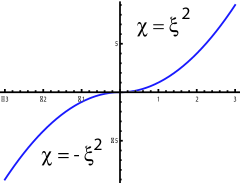
Figure 1: Tangential continuity during the focusing process. The function takes a different form when the variable $\chi$ passes from negative to positive values. Yet the transition is continues with continuous first derivatives. Their second derivatives take different forms. Thus, it is a tangential but not analytic continuation.

When $\chi=0$,

$$\frac{1}{x_{1}}+\frac{1}{x_{2}}=1.$$ (16)

the camera is focused, and the matrix becomes

$$\pmatrix{1&0\cr 1&1}.$$ (17)

During the focusing process, the upper right component of the camera matrix goes from a negative value to a positive value, which is a continuous process, as demonstrated in Fig.1. The second derivatives is not continuous, therefore this kind of continuity is not analytic. Nevertheless, since the first derivatives are continuous, the process is tangentially continuous.

If $x_{2}$ is $x_{0}$, where

$$x_{0}=\frac{x_{1}}{x_{1}-1},$$ (18)

the camera is focused. If $x_{1}$ is very large, $x_{0}$ approaches the focal length. If $x_{1}$ is smaller than $x_{0}$, $\chi$ is negative, and the camera matrix take the form of Eq.(14). If $x_{1}$ is larger than $x_{0}$, the camera matrix takes the form of Eq.(15).

2.3 Mathematical Summary

In this section, we were first interested in achieving the equi-diagonalization of the two-by-two matrix without changing the off-diagonal elements. For this purpose, we used a Hermitian transformation which produces a scale change on the diagonal elements.

It was then noted that the focusing process corresponds the transiton from Eq.(14) to Eq.(15). Their traces are smaller and greater than 2, respectively. As shown in Fig. LABEL:xsq, this results in the “soldering” of two different functions. The the functions and their first derivatives are continuous at the point where they are glued together and consequently the property is termed as tangentially continuous.

In our earlier papers, we studied the $ABCD$ matrix applicable to periodic systems such as laser cavities, where the equi-diagonalization is achieved through a similarity transformation by using rotations. Since the inverse of the rotation matrix is also its Hermitian conjugate, we can put both the scale transformation and the rotation into one set of Hermitian trasformations.

3 The Equi-diagonalization and the Continuity of the $ABCD$ matrix

The $ABCD$ matrices are essential in understanding the propagation of light, both in ray optics and Gaussian beam optics. Its determinant is one for lossless systems. For paraxial ray optics, this two-by-two matrix has real components, and in view of the condition on its determinant the number of independent components reduces to three.

Therefore, from a group theoretical point of view, it can be represented in terms of the symplectic group $Sp(2)$, consisting of one rotation and two squeeze matrices, whose properties have been extensively discussed in connection with its applicability to optics. [4]

It was noted in our earlier publications that this matrix cannot always be diagonalized, but it can be brought to a form with equal diagonal elements. This equi-diagonal form can serve many useful computational purposes.

We noted further that the $ABCD$ matrix can be brought to an equi-diagonal form by a rotation. As was noted in Sbsec. 2.3, this rotation and the scale change in lens optics can be grouped into a set of Hermitian transformations.

Furthermore, it was shown in one of our earlier papers that the equi-diagonalized matrix can be expressed in an exponential form with two matrix generators and one angular parameter. Depending on the values of this parameter, the matrix has four branches. [5] However, we noted that the $ABCD$ matrix maintains its continuity while crossing from one branch to another. We noted there that it is not an analytic continutation, but we could not go further than that. In this section, we shall conclude that this continuity is the tangential continuity as discussed in Sec. 2.

We shall discuss the problems of equi-diagonalization in full detail in Sec. 3.1.

3.1 Equi-diagonalization of the $ABCD$ matrix

The $ABCD$ matrix can not always be brought into a diagonal form, but it is possible to bring it into an equi-diagonal form by rotations [4]

$$[abcd]_{R}=R(-\sigma/2)[ABCD]R(\sigma/2),$$ (19)

where the $ABCD$ and the $[abcd]$ matrices are of the form

$$[ABCD]=\pmatrix{A&B\cr C&D},\qquad[abcd]=\pmatrix{a&b\cr c&d},$$ (20)

respectively, and $R(\sigma)$ is

$$\pmatrix{\cos(\sigma/2)&-\sin(\sigma/2)\cr\sin(\sigma/2)&\cos(\sigma/2)}$$ (21)

is the rotation matrix. Here $(abcd)_{R}$ denotes the equi-diagonal matrix achieved by rotations, and $a,b,c$ and $d$ can be expressed in terms of the elements of Eq.(20) where

$$\tan\sigma=\frac{A-D}{B+C}.$$ (22)

However, transformations by rotations are not the only way to bring it to an equi-diagonal form. They can also be equi-diagonalized by squeeze matrices as

$$[abcd]_{S}=S(\gamma/2)[ABCD]S(\gamma/2),$$ (23)

where $S(\gamma)$ is

$$\pmatrix{e^{\gamma/2}&0\cr 0&e^{-\gamma/2}},$$ (24)

and the squeeze parameter

$$e^{\gamma}=\sqrt{D/A},$$ (25)

with

$$a=d=\sqrt{AD},\quad b=B,\quad c=C,$$ (26)

if $A$ and $B$ have the same sign.

We now have two different transformation matrices. One is the rotation matrix and the other is the squeeze matrix. It is possible to accommodate both in a single form by a Hermitian transformation

$$L[ABCD]L^{\dagger}.$$ (27)

where $L^{\dagger}$ is the Hermitian conjugate of $L$. The rotation matrix is antisymmetric and its Hermitian conjugate is its inverse. Thus, it is a similarity transformation. The squeeze matrix is symmetric, and it is invariant under the Hermitian conjugation. The Hermitian transformation of Eq.(27) is not a similarity transformation. The usage of rotations is far well known in optical sciences compared to the usage of squeeze transformations, which are also well established in the context of special relativity. [4, 9, 10]

Thus, equi-diagonalization is possible through transformations

$$M[ABCD]M^{-1},\quad\mbox{or}\quad M[ABCD]M^{\dagger},$$ (28)

where $M$ is a two-by-two matrix from the group $Sp(2)$. If the matrix $M$ is antisymmetric, its Hermitian conjugate is its inverse. If it is symmetric, it is invariant under the conjugation, but conjugation does yield its inverse. In either case, there is a variety of ways bringing the $ABDC$ matrix to a diagonal form. We can choose the method depending on our purpose.

Now, let us go back to the procedure from Eq.(6) to Eq.(7). This is a translation operation which will place the lens exactly halfway between the image and object. This is achieved by the similarity transformation of a triangular matrix in the form

$$\pmatrix{1&\kappa\cr 0&1}.$$ (29)

On the other hand, this triangular matrix can be obtained by multiplications of the squeeze and rotation matrices in the Sp(2) group. This process is known as the Iwasawa decomposition. [11, 12] However, this process of equi-diagonalization does not leave the off-diagonal elements invariant, and thus is not useful for focusing processes.

3.2 Tangential continuity of the $ABCD$ matrix

It was shown also in our previous paper [5] that the equi-diagonal form of the $ABCD$ matrix can be written in the exponential form

$$[abcd]=\exp{\left[-ir(A\cos\theta+S\sin\theta)\right]},$$ (30)

where

$$A=\pmatrix{0&-i\cr i&0},\qquad S=\pmatrix{0&i\cr i&0}.$$ (31)

Then, we have

$$[abcd]=\exp{\left[r\pmatrix{0&-\cos\theta+\sin\theta\cr\cos\theta+\sin\theta&0}\right]}.$$ (32)

Let us next consider the new angle variable defined as

$$\alpha=\theta-\frac{\pi}{4}.$$ (33)

Then the above exponential form can be written as

$$[abcd]=\exp{\left[\sqrt{2}r\pmatrix{0&\sin\alpha\cr\cos\alpha&0}\right]}.$$ (34)

Now, the $[abcd]$ matrix is to be investigated for various values of the angle $\alpha$.

Case i)  The angle $\alpha$ is smaller than $0$ but larger than $-\pi/2$:
Within this range of $\alpha$ the exponent of Eq.(34) can be expressed as

$$r\sqrt{\sin(2|\alpha|)}\pmatrix{0&-e^{-\eta}\cr e^{\eta}&0}$$ (35)

which can also be written as a similarity transformation

$$r\,\,\sqrt{\sin(2|\alpha|)}\pmatrix{e^{-\eta/2}&0\cr 0&e^{\eta/2}}\pmatrix{0&-1\cr 1&0}\pmatrix{e^{\eta/2}&0\cr 0&e^{-\eta/2}},$$ (36)

where

$$e^{-\eta}=\sqrt{\tan(|\alpha|)}.$$ (37)

It is apparent that the $[abcd]$ matrix is a similarity transformation of an exponential

$$[abcd]=\pmatrix{e^{-\eta/2}&0\cr 0&e^{\eta/2}}\exp{\left[\rho_{-}\pmatrix{0&-1\cr 1&0}\right]}\pmatrix{e^{\eta/2}&0\cr 0&e^{-\eta/2}}$$ (38)

where

$$\rho_{-}=r\sqrt{\sin(2|\alpha|)}.$$ (39)

After exponentiating the matrix becomes

$$[abcd]=\pmatrix{\cos\rho_{-}&-e^{-\eta}\sin\rho_{-}\cr e^{\eta}\sin\rho_{-}&\cos\rho_{-}}.$$ (40)

Now, it is possible to express the group parameters $\eta$ and $\rho_{+}$ in terms of the physical quantities of the camera like one lens system $d_{1},d_{2}$ and $f$ as

$$e^{\eta}=\frac{1}{\sqrt{|\chi|}},\qquad-(\sin\rho_{-})^{2}=-|\chi|$$ (41)

where $\chi$ is given as in Eq.(10).

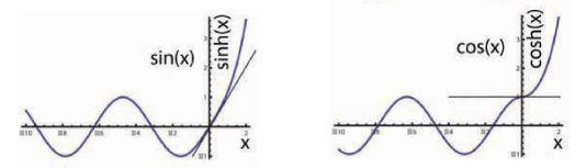
Figure 2: Transitions from $\sin(x)$ to $\sinh(x)$, and from $\cos(x)$ to $\cosh(x)$ at $x=0$. They are continuous transitions. Their first derivatives are also continuous. However, their second and third derivatives take different forms. They are thus tangentially continuous transitions.

Case ii)  The angle $\alpha$ is larger than $0$ but less than $\pi/2$:
Within this range of $\alpha$ the exponent in Eq(34) is expressed as

$$r\,\,\sqrt{\sin(2\alpha)}\pmatrix{e^{-\eta/2}&0\cr 0&e^{\eta/2}}\pmatrix{0&1\cr 1&0}\pmatrix{e^{\eta/2}&0\cr 0&e^{-\eta/2}}.$$ (42)

After exponentiating, as before, the $[abcd]$ matrix takes the form

$$[abcd]=\pmatrix{\cosh\rho_{+}&e^{-\eta}\sinh\rho_{+}\cr e^{\eta}\sinh\rho_{+}&\cosh\rho_{+}},$$ (43)

where

$$e^{-\eta}=\sqrt{\tan(\alpha)},\qquad\rho_{+}=r\sqrt{\sin{(2\alpha)}}.$$ (44)

Similarly, as in the case above the group parameters are related to the physical quantities as:

$$e^{\eta}=\frac{1}{\sqrt{\chi}},\qquad(\sinh\rho_{+})^{2}=\chi.$$ (45)

Now, Eq.(40) and Eq.(43) can be combined into one exponential form by

$$\exp{\left[\rho_{\pm}\pmatrix{0&\pm e^{-\eta}\cr e^{\eta}&0}\right]}.$$ (46)

To examine the transition between Eq.(40) and Eq.(43), Eq.(6) is expanded around small values of $\alpha$, for the cases (i) and (ii). They become

$$\pmatrix{1-|\alpha|r^{2}&-\sqrt{2}r|\alpha|\cr\sqrt{2}r&1-|\alpha|r^{2}},\qquad\pmatrix{1+\alpha r^{2}&\sqrt{2}r\alpha\cr\sqrt{2}r&1+\alpha r^{2}}$$ (47)

respectively. They attain the same form when $\alpha=0$, where both are lower triangular matrices, with vanishing upper right components similar to that of Eq.(17), accounting for the focusing procedure.

The tangential continuity is illustrated in Fig. 2, where the transition from trigonometric to hyperbolic functions are presented, with their common tangential lines.

Conclusion

Our study on the equi-diagonalization and thereafter the branching property of the $ABCD$ matrix was initiated while investigating the behavior of light rays in periodic systems such as laser resonators and multilayer optics, in our earlier papers. [5] In those papers we have also given the relations between the group parameters and group parameters.

We have further noted that the equi-diagonal matrix can have its trace smaller than 2, greater than 2, or equal to 2, and that the transition from one branch to another is continuous, but we were not able to clarify the nature of the continuity.

In this paper, we used lens optics to study this problem, and concluded that the answer is the “tangential continuity.” However, there are some intricacies due to different procedures for equi-diagonalization.

For lens optics, we used the Hermtian transformation of the form $L[ABCD]L^{\dagger}$, while the similarity transformation of the form $S[ABCD]S^{-1}$ is applicable to the periodic systems discussed in Sec. 3. The similarity transformation is well known and possesses the property

$$\left[M[ABCD]M^{-1}\right]^{n}=M[ABCD]^{n}M^{-1},$$ (48)

which is needed for dealing with periodic systems.

The Hermitian transformation is rare in the literature, but it is not new. It is applicable to Lorentz transformations of the spacetime four-vectors in the two-by-two representation. [4]

While these two transformations perform different mathematical operations, transformations by rotations belong to both types. We use rotations as a subset of the similarity transformation in Sec. 3. Since the Hermitian transformation also contains this subset, we can include both equi-diagoanalization processes into one set of Hermitian transformations.

The concept of tangential continuity in lens optics is directly applicable to the $ABCD$ matrices discussed in Sec. 3 for periodic systems such as laser optics and multilayer optics. Indeed, in this paper, we have completed our investigation of the continuity problem in the transition from one branch of the $ABCD$ matrix to another, which was left unresolved in our earlier paper in this journal.[5].

References

- [1] Marhic, M. E. J. Opt. Soc. Am. A 1995, 12, 1448-1459.
- [2] Bastiaans, M. J.; Alieva, T. J. Opt. Soc. Am. A 2006, 23, 1875-1883.
- [3] Bastiaans, M. J.; Alieva, T. J. Opt. Soc. Am. A 2007, 24, 1053-1062.
- [4] Başkal, S.; Kim, Y. S. Mathematical Optics, Classical, Quantum and Computational Methods; 2013 edited by V. Lakshminarayanan, M. L. Calovo, T. Alieva, CRC Press, Boca Raton, 303-340.
- [5] Başkal, S.; Kim, Y. S. J. Mod. Opt. 2010, 57, 1251-1259.
- [6] Saleh, B. E. A.; Teich, M. C. Fundamentals of Photonics John Wiley Sons, Inc., Hoboken, New Jersey, 2007.
- [7] Başkal, S.; Kim, Y. S. Phys. Rev. E 2003, 67, 56601-56608.
- [8] Georgieva, E.; Kim, Y. S. Phys. Rev. E 2003, 68, 26606-26612.
- [9] Naimark, M. A. Linear Representations of the Lorentz Group, translated from Russian by Ann Swinfen and O. J. Marstrand, Pergamon Press, 1964.
- [10] Kim, Y. S.; Noz, M. E. Symmetry 2013, 5, 233-252.
- [11] Iwasawa, K. Annals of Mathematics 1949, 50, 507-558.
- [12] Başkal, S.; Kim, Y. S. Phys. Rev. E 2001, 63, 056606-056611.