Transversity Distribution Functions in the Valon Model

Abstract

We use the valon model to calculate the transversity distribution functions , inside the Nucleon. Transversity distributions indicate the probability to find partons with spin aligned (anti- aligned) to the transversely polarized nucleon. The results are in good agreements with all available experimental data and also global fits.

1 Introduction

The nucleon ”spin crisis” is still one of the most fundamental problems in high energy spin physics. Results of Deep Inelastic Scattering (DIS) experiments suggest that just $30\%$ of the spin of the proton is carried by the intrinsic spin of its quark constituents. This discovery has challenged our understanding about the internal structure of the proton. Therefore many theoretical and experimental studies have been conducted to investigate and understand the role of spin in the proton’s internal structure.
The key question is how the spin of the nucleon is shared among its constituent quarks and gluons. That is, the determination and understanding of the shape of quarks and gluon spin distribution functions have become an important task.
In general, there are three collinear parton distribution functions: the unpolarized parton distribution functions (PDFs), the longitudinally polarized distribution functions (PPDFs) and the transversity distributions . They are defined as follows: if we show the number density of quarks with helicity $\pm 1$ inside a positive hadron with $q_{\pm}(x,Q^{2})$, then we have:

$$q(x,Q^{2})=q_{+}(x,Q^{2})+q_{-}(x,Q^{2})$$ (1)

$$\Delta q(x,Q^{2})=q_{+}(x,Q^{2})-q_{-}(x,Q^{2})$$ (2)

where $q(x,Q^{2})$ is the probability of finding a parton with fraction $x$ of parent hadron momentum and $\Delta q(x,Q^{2})$ represents the probability of finding a polarized parton with fraction $x$ of parent hadron momentum and spin align/anti-align to hadron’s spin. It measures the net helicity of partons in a longitudinally polarized hadron.
The third parton distributions are transversity distribution functions. They have a simple meaning too: In a transversely polarized hadron, transversity distribution is denoted by $\Delta_{T}q(x,Q^{2})$ and represents the number density of partons with momentum fraction $x$ and polarization parallel to that of the hadron minus the number density of partons with the same momentum fraction and antiparallel spin direction:

$$\Delta_{T}q(x,Q^{2})=q_{\uparrow}(x,Q^{2})-q_{\downarrow}(x,Q^{2})$$ (3)

Historically they were first introduced in 1970’s by Ralston and Soper [1] and rediscovered by Artru and Mekhfi [2] in the beginning of 90’s and their QCD evolution studied by Jaffe and Ji [3].
Since $\Delta_{T}q(x,Q^{2})$ is a chirally-odd quantity, it can not be probed in the cleanest hard process, DIS. It can only be accessed in process where it couples to another chirall-odd quantity. As such, $\Delta_{T}q(x,Q^{2})$ can be measured in hard reactions such as semi-inclusive leptoproduction or in the Drell-Yan di-muon production. Measuring the transverse polarization of partons are the goal of experiments such as COMPASS, HERMES, RHIC and SMC Collaborations [4, 5, 6]. These measurements can teach us about the transvesity distribution and the transverse motion of quarks and thus the role that their orbital angular momentum play in the structure of proton and fragmentation processes.
Calculation of transversity distribution functions, using some phenomenology is an active task in spin physics [7, 8, 9, 10]. We intend to do the same and calculate transversity distribution using the Valon model. The valon model is a phenomenological model originally proposed by R. C. Hwa, [11] in early 80’s. It was improved later by Hwa [12] and Others [13, 14, 15] and extended to the polarized cases [16, 17, 18]. In this model a hadron is viewed as three (two) constituent quark-like objects, called valons. Each valon is defined to be a dressed valence quark with its own cloud of sea quarks and gluons. The dressing processes are described by QCD. The structure of a valon is resolved at high $Q^{2}$. At low $Q^{2}$, a valon behaves as constituent quark of the hadron. In this model the recombination of partons into hadrons is a two stage process: in the first step the partons emit and absorb gluons in the process of the evolution of the quark- gluon cloud and become ”valons”; then these valons recombine into hadron. The model describes the un-polarized and polarized nucleon structure rather well [15, 18].
In the present paper we apply the valon concept to the transverse polarization and calculate the transversity distribution functions. The paper is organized as follows. In Section 2 we review the valon model for calculating the polarized parton distribution functions(PPDFs). Then in Section 3 we utilize it to calculate the transversity distribution. Our conclusions are given in Section 4.

2 Polarized parton distribution functions in the valon model

In the valon representation of hadrons the polarized parton distribution in a polarized hadron is given by:

$$\delta q_{{i}}^{\it{h}}(x,Q^{2})=\sum\int_{x}^{1}\frac{dy}{y}\delta G_{\it{valon}}^{h}(y)\delta q_{{i}}^{\it{valon}}(\frac{x}{y},Q^{2})$$ (4)

where $\delta G_{\it{valon}}^{h}(y)$ is the helicity distribution of the valon in the hosting hadron i.e (probability of finding the polarized valon inside the polarized hadron). Here we study the internal structure of proton, so we have to use the polarized valon distributions inside proton. $\delta G_{\it{valon}}^{p}(y)$ is related to unpolarized valon distribution, $G_{j}^{p}(y)$ by:

$$\delta G_{j}^{p}(y)=\delta F_{j}(y)G_{j}^{p}(y)=N_{j}y^{\alpha_{j}}(1-y)^{\beta_{j}}(1+a_{j}y^{0.5}+b_{j}y+c_{j}y^{1.5}+d_{j}y^{2})$$ (5)

where $j$ refers to U and D type valons [11, 15]. Polarized valon distributions are determined by a phenomenological argument [16]. The parameters in Eq. (5) are summarized in Table (1) and $\delta G_{\it{valon}}^{p}(y)$ are plotted in Figure (1). The term $\delta q_{{i}}^{\it{valon}}(x/y,Q^{2})$ for $h=p$ in Eq. (4) is the polarized parton distribution inside a valon. Their evolution are governed by the DGLAP equations [19, 20, 21]. Finally, the polarized proton structure functions are obtained via a convolution integral as follows:

$$g^{p}_{1}(x,Q^{2})=\sum_{\it{valon}}\int_{x}^{1}\frac{dy}{y}\delta G_{\it{valon}}^{p}(y)g^{\it{valon}}_{1}(\frac{x}{y},Q^{2})$$ (6)

where $g^{\it{valon}}_{1}(\frac{x}{y},Q^{2})$ is the polarized structure function of the valon. The details of the actual calculations are given in [16, 17, 18].

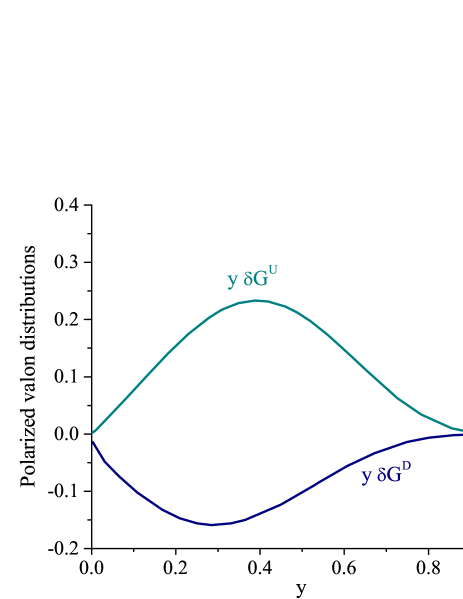
Figure 1: (color online) Polarized valon distributions for U and D valons inside the proton.

$valon(j)$	$N_{j}$	$\alpha_{j}$	$\beta{{}_{j}}$	$a_{j}$	$b_{j}$	$c_{j}$	$d_{j}$
$U$	3.44	0.33	3.58	-2.47	5.07	-1.859	2.780
$D$	-0.568	-0.374	4.142	-2.844	11.695	-10.096	14.47

Table 1: Numerical values of the parameters in Eq. (5) for polarized valon distributions inside proton.

3 Transversity Distribution Functions in the valon model

We now follow the same procedure as in Section 2, to calculate the transversity distribution functions of partons in the proton. For the transversely polarized proton, Eq. (4) reads as:

$$\Delta_{T}q_{{i}}^{\it{p}}(x,Q^{2})=\sum_{valons}\int_{x}^{1}\frac{dy}{y}\Delta_{T}G_{\it{valon}}^{p}(y)\Delta_{T}q_{{i}}^{\it{valon}}(\frac{x}{y},Q^{2})$$ (7)

where $\Delta_{T}G_{valon}^{p}(y)$ is the transverse valon distribution functions describing the probability of finding a valon with spin aligned or anti-aligned with the transversly polarized proton. In fact, $\Delta_{T}G_{valon}^{p}(y)$ is identical to $\delta G_{\it{valon}}^{p}(y)$ in the longitudinal case. This is so, because we know that in the non-relativistic limit of the quark motion, the PPDFs and transversity distribution would be identical, since the rotations and Euclidean boosts commute and a series of boosts and rotation can convert a longitudinal polarized proton into a transversely polarized one with an infinite momentum [9, 22]. The only difference between the transversity distributions and PPDFs reflects the relativistic character of quark motion in the proton and shows up in the splitting functions and DGLAP equations. Consequently, here we set $\Delta_{T}G_{valon}^{p}(y)=\delta G_{\it{valon}}^{p}(y)$. Also notice that $\Delta_{T}q_{i}^{valon}(\frac{x}{y},Q^{2})$ in Eq. (7) are the transversity distribution functions in the valon. They can be calculated using the DGLAP evolution equations, as described bellow.
In the Mellin space, transversity distribution functions are given by:

$$\Delta_{T}q_{\pm}(n)=\Delta_{T}q(n)\pm\Delta_{T}\overline{q}(n)$$ (8)

where $\Delta_{T}q_{\pm}(n)$ are the Singlet and Non-Singlet transversity distribution functions of partons. The first moment (n=1) of transversity distribution refers to the proton’s tensor charge [23, 24, 25]. Their DGLAP evolution equations are [26]:

$$\frac{d}{d\ln Q^{2}}\Delta_{T}q_{-}(n,Q^{2})=\Delta_{T}\gamma_{qq,-}(n,\alpha_{s}(Q^{2}))\Delta_{T}q_{-}(n,Q^{2})$$ (9)

$$\frac{d}{d\ln Q^{2}}\Delta_{T}q_{+}(n,Q^{2})=\Delta_{T}\gamma_{qq,+}(n,\alpha_{s}(Q^{2}))\Delta_{T}q_{+}(n,Q^{2})$$ (10)

The solution of the DGLAP evolution equations in the Mellin space at NLO approximation are [27]:

$$\Delta_{T}q_{\pm}(n,Q^{2}) = \{1+\frac{\alpha_{s}(Q_{0}^{2})-\alpha_{s}(Q^{2})}{\pi\beta_{0}}[\Delta_{T}\gamma_{qq,\pm}^{(1)}(n)-\frac{\beta_{1}}{2\beta_{0}}\Delta_{T}\gamma_{qq}^{(0)}(n)]\}$$ (11)

$$\times(\frac{\alpha_{s}(Q^{2})}{\alpha_{s}(Q_{0}^{2})})^{\frac{-2\Delta_{T}\gamma_{qq}^{(0)}(n)}{\beta_{0}}}\Delta_{T}q_{\pm}(n,Q_{0}^{2}),$$

In the above equation, $\Delta_{T}q_{\pm}(n,Q_{0}^{2})$ are the initial input densities. They are determined by a phenomenological argument in the valon model. $\Delta_{T}\gamma_{qq,\pm}^{(0)}(n)$ and $\Delta_{T}\gamma_{qq,\pm}^{(1)}(n)$ are the usual anomalous dimensions and are given in Appendix A.
In the following, first we solve the DGLAP evolution equations for a valon. This will give transversity distribution functions in each valon. We then use them in the convolution integral, Eq. (7) to obtain transversity distribution functions in the proton. In doing so, we adopt the $\overline{MS}$ scheme with $\Lambda_{QCD}=0.22$ $GeV$ and $Q_{0}^{2}=0.283$ $GeV^{2}$. This value of $Q_{0}^{2}$ corresponds to a distance of $0.36fm$ which is roughly equal to or slightly less than the radius of a valon. It may be objected that such distances are probably too large for a meaningful pure perturbative treatment. We note that valon structure function has the property that it becomes $\delta(z-1)$ as $Q^{2}$ is extrapolated to $Q_{0}^{2}$ , which is beyond the region of validity. This mathematical boundary condition signifies that the internal structure of a valon cannot be resolved at $Q_{0}^{2}$ in the NLO approximation. Consequently, when this property is applied to Eq. (7), the structure function of the nucleon becomes directly related to $x\delta_{T}G^{valon}$ at those values of $Q_{0}^{2}$. Furthermore, as noted in [15], we have checked that when $Q^{2}$ approaches $Q_{0}^{2}$, the quark moments approach to unity and gluon moments go to zero. From the theoretical standpoint, both $\Lambda_{QCD}$ and $Q_{0}^{2}$ depend on the order of the moments, but here, we have assumed that they are independent of moment order. In this way, we have introduced some degree of approximation to the $Q^{2}$ evolution of the valence and sea quarks. However, on one hand there are other contributions like target-mass effects, which add uncertainties to the theoretical predictions of perturbative QCD, while on the other hand since we are dealing with the valons, there is no experimental data to invalidate moment order independent of $\Lambda_{QCD}$. Therefore we led to choose our initial input densities at $Q_{0}^{2}$ to be $\delta(z-1)$, leading to:

$$\Delta_{T}q_{+}(z,Q_{0}^{2})=\Delta_{T}q_{-}(z,Q_{0}^{2})=\delta(z-1)$$ (12)

Thus, their moments are

$$\Delta_{T}q_{+}(n,Q_{0}^{2})=\Delta_{T}q_{-}(n,Q_{0}^{2})=\int^{1}_{0}z^{n-1}\delta(z-1)dz=1$$ (13)

It is also interesting to note that our selected value for $Q_{0}^{2}$ is very close to the transition region reported by the CLAS Collaboration for the behavior of the first moment of the proton structure function around $Q^{2}=0.3\ GeV^{2}$ [28].
The moments of valence quark transversity distribution is now easily obtained from the solution of DGLAP evolution equations, Eq. (11), in Mellin space; as they are shown in figure (2). Finding the transversity distribution functions in a valon, using Eq. (11), is now reduced to an inverse Mellin transformation. This enable us with the help of Eq. (7) to obtain $x\Delta_{T}u(x)$ and $x\Delta_{T}d(x)$ as a function of x. They are shown in figure (3) for a number of $Q^{2}$-values.

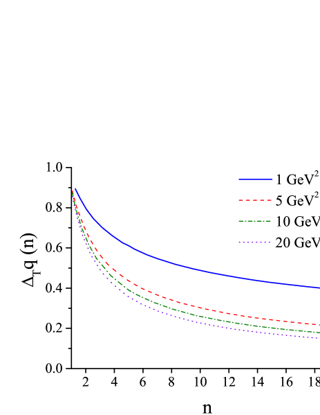
Figure 2: (color online) $\Delta_{T}q(n)$ as a function of n in different ranges of $Q^{2}$ .

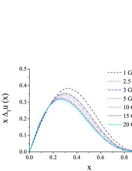
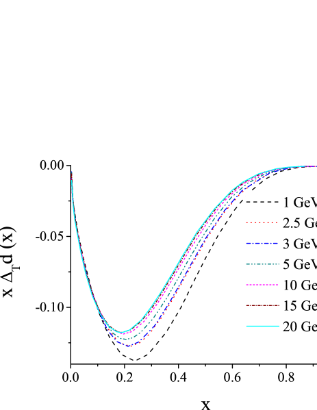
Figure 3: (color online) $x\Delta_{T}u(x)$ and $x\Delta_{T}d(x)$ as a function of x for different ranges of $Q^{2}$ .

It is common to write the transversity distribution functions as:

$$\Delta_{T}q(x)=\int\Delta_{T}q(x,k_{\bot})\ d^{2}k_{\bot}$$ (14)

where $\Delta_{T}q(x,k_{\bot})$ are the un-integrated transversity distribution functions. We assume that $k_{\bot}$ dependence of transversity distributions are factorized in a Gaussian form:

$$\Delta_{T}q(x,k_{\bot})=\Delta_{T}q(x)\frac{e^{\frac{-k_{\bot}^{2}}{\langle k_{\bot}^{2}\rangle}}}{\pi\langle k_{\bot}^{2}\rangle},$$ (15)

where $\Delta_{T}q(x)$ is transverse distribution function and the average values of $k_{\bot}$ is taken from SIDIS cross section data [29, 30], to be

$$\langle k_{\bot}^{2}\rangle=0.25\ GeV^{2}$$ (16)

In figure (4), We show our results for the transversity distribution function of the valence u quark , $x\Delta_{T}u(x,Q^{2})$. It is compared with Anselmino 2008 and Soffer ’s global fits at $Q^{2}=2.4\ GeV^{2}$ [9, 31]. We also show the result for $x\Delta_{T}u(x,k_{\bot})$ distribution at $x=0.1$ in the right panel of figure (4) . The same plot is given for d valence quark in figure (5). Figure (6) shows a more recent global fit results [10] as compared to our analysis.

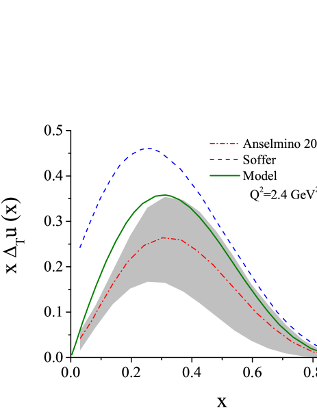
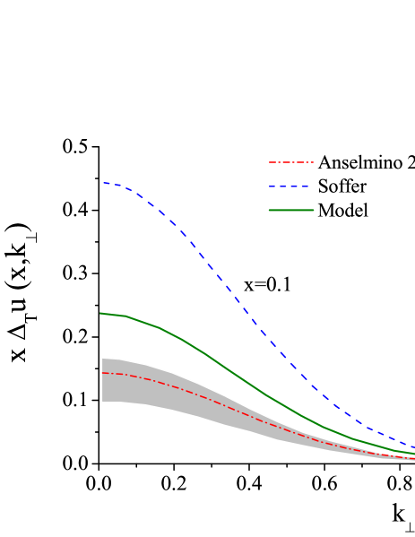
Figure 4: (color online) The transversity distribution function for valence u quark calculated by our model as a function of x and $k_{\bot}$ at $Q^{2}=2.4\ GeV^{2}$ . They are compared with those from Soffer and Anselmino global fits [9, 31].

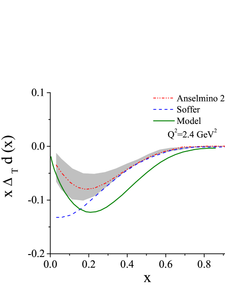
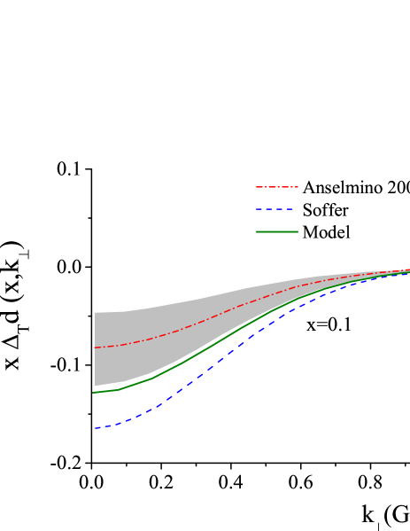
Figure 5: (color online) The transversity distribution function for valence d quark calculated by our model as a function of x and $k_{\bot}$ at $Q^{2}=2.4\ GeV^{2}$ . They are compared with those from Soffer and Anselmino global fits [9, 31].

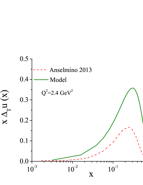
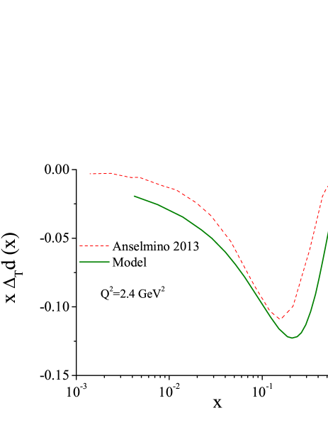
Figure 6: (color online) The transversity distribution functions for valence u and d quarks in our model as a function of x and at $Q^{2}=2.4\ GeV^{2}$ and comparison with Anselmino fit (2013)[10].

In figure (7) we present the result for $x[\Delta_{T}u_{v}(x,Q^{2})-\frac{1}{4}\Delta_{T}d_{v}(x,Q^{2})]$ and compare with those reported by HERMES and COMPASS Collaborations [32, 33], as well as Radici ’s model [34] .

Figure 7: (color online) The combination of transversity distribution functions for valence u and d flavors . Black circles for SIDIS data from HERMES [32] , red squares from CAMPASS [33] and Green curve is obtained by our model at $Q^{2}=2.5\ GeV^{2}$ . Blue curve shows the result of Radici ’s model [34] with its associated uncertainty band which represents the same observable as deduced from the parametrization of Ref[35]

.

Another interesting quantity, related to the first moment is the tensor charge, defined by the integral (17) as :

$$\delta q=\int_{0}^{1}dx\ (\Delta_{T}q-\Delta_{T}\overline{q})$$ (17)

In our analysis the first moment of sea transversity distributions turn out to be very small: $(-0.00105)$ for $Q^{2}=1GeV^{2}$. Therefore, the tensor charges are absolutely the first moment of valence transversity distribution functions. Actually the valon model predicts that the sea quark polarization are very small and are consistent with zero. It is undetectable, since the valon structure is generated by perturbative dressing in QCD. In such processes with massless quarks, helicity is conserved and therefore, the hard gluons can not induce sea quark polarization perturbatively. The experiments also support this finding [36, 37, 38, 39]. Thus we have no sea polarization in our model. As a consequence, the first moment of transversity distributions of u and d quark(Tensor charges ) at $Q^{2}=1GeV^{2}$ are:

$$\delta u=0.7386\ ,\ \delta d=-0.3782$$ (18)

Finally, in figure (8) our results for tensor charge are compared with the predictions of some models [9, 10, 40, 41, 42, 43, 44].

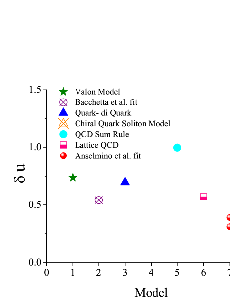
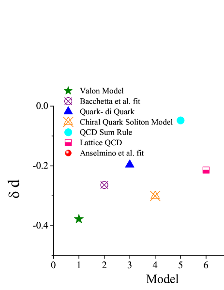
Figure 8: (color online) The tensor charge for $u$ and $d$ quarks. Our prediction is shown by number one and compared with those from several models [10, 40, 41, 42, 43, 44].

4 Conclusions and Remarks

We have utilized the so called valon model and calculated Transversity distribution functions for u and d quarks inside the proton. The transversity distribution functions together with the helicity distribution functions provide a more comprehensive picture of the proton structure. While the former is fairly well understood, the latter is just beginning to be probed. Our calculation in this paper is a step towards this goal. As noted in Eq. (18) of the text, in our model the sea partons contribution to the transversity distributions is consistent with zero, whereas the valence sector assumes a sizeable value. In a sense, this prediction is similar to the one we have made for the helicity distribution in Reference [16], which later on confirmed by experiment. However, the obtained results do not exhaust the spin of proton and implies that there is room for further contribution from perhaps, the orbital angular momentum. It also shows that a simple model like valon reasonably well reproduces the experimental data and hence provide a physical picture of the proton structure in the NLO approximation.

Appendix

Here we list the anomalous dimensions in mellin space and $\overline{MS}$ scheme: [45]

the $\gamma^{(0)}(n),\gamma^{(1)}(n)$ adequate to $\Delta_{T}q$ are as follows:

$$\Delta_{T}\gamma_{qq}^{(0)}(n)=C_{F}[\frac{3}{2}-2\sum_{j=1}^{n}\frac{1}{j}]$$ (19)

$$\Delta_{T}\gamma_{qq,\eta}^{(1)}(n) = C_{F}^{2}\{\frac{3}{8}+\frac{2}{n(n+1)}\delta_{\eta-}-3S_{2}(n)-4S_{1}(n)[S_{2}(n)-\acute{S}_{2}(\frac{n}{2})]$$ (20)

$$-8\tilde{S}(n)+\acute{S}_{3}(\frac{n}{2})\}$$

$$+\frac{1}{2}C_{F}N_{c}\{\frac{17}{12}-\frac{2}{n(n+1)}\delta_{\eta-}-\frac{134}{9}S_{1}(n)+\frac{22}{3}S_{2}(n)$$

$$+4S_{1}(n)[2S_{2}(n)-\acute{S}_{2}(\frac{n}{2})]+8\tilde{S}(n)-\acute{S}_{3}(\frac{n}{2})\}$$

$$+\frac{2}{3}C_{F}T_{F}\{-\frac{1}{4}+\frac{10}{3}S_{1}(n)-2S_{2}(n)\},$$

where $\eta=\pm$ and the S (Harmonic Functions) are defined by ;

$$S_{k}(n) \equiv \sum_{j=1}^{n}\frac{1}{j^{k}}$$ (21)

$$S_{k}^{\prime}\left(\frac{n}{2}\right) \equiv 2^{k-1}\sum_{j=1}^{n}\frac{1+(-)^{j}}{j^{k}}=\frac{1}{2}(1+\eta)S_{k}\left(\frac{n}{2}\right)+\frac{1}{2}(1-\eta)S_{k}\left(\frac{n-1}{2}\right)$$ (22)

$$\tilde{S}(n) \equiv \sum_{j=1}^{n}\frac{(-)^{j}}{j^{2}}S_{1}(j)$$ (23)

$$= -\frac{5}{8}\zeta(3)+\eta\left[\frac{S_{1}(n)}{n^{2}}+\frac{\pi^{2}}{12}G(n)+\int_{0}^{1}dx\;x^{n-1}\frac{{\rm{Li}}_{2}(x)}{1+x}\right]$$

with $G(n)\equiv\psi\left(\frac{n+1}{2}\right)-\psi\left(\frac{n}{2}\right)$, $\psi(z)=d\ln\Gamma(z)/dz$ and $\eta=\pm 1$ for $\delta P_{NS\pm}^{(1)n}$ and $\eta=-1$ for the flavor singlet anomalous dimensions.

References

- [1] J.Ralston and D.E.Soper, Nucl.Phys B 152 (1979) 109
- [2] X. Artru, M. Mekhfi, Nucl. Phy. A 532 (1991) 351-358
- [3] R. L. Jaffe and X. Ji, Phy. Rev. Lett. 67. 552 (1991); Phy. Rev. Lett. 71. 2547 (1993)
- [4] C. Schill, on behalf of the COMPASS collaboration, Nuclear Physics B (Proc. Suppl.) 207-208 (2010) 49 52
- [5] HERMES Collaboration, Physics Letters B 693 (2010) 11-16
- [6] G. Schnell, Nuclear Physics B (Proc. Suppl.) 222-224 (2012) 187-198
- [7] A.V.Efremov, Annalen Phys. 13(2004) 651-664 [hep-ph/0410389]
- [8] S. Scopetta, V. Vento, Phys. Lett. B 424 (1998) 25-32
- [9] M. Anselmino, M. Boglione, U. D’Alesio, A. Kotzinian, S. Melis, F. Murgia and A. Prokudin, Nucl. Phys. Proc. Suppl. 191 (2009) 98–107, [hep-ph/0812.4366]
- [10] M. Anselmino, M. Boglione, U. D’Alesio, A. Kotzinian, S. Melis, F. Murgia and A. Prokudin, Phys. Rev. D 87 094019 (2013)
- [11] R. C. Hwa, Phys. Rev. D 22, 759 (1980)
- [12] R. C. Hwa, Phys. Rev. D 51, 85 (1995)
- [13] R. C. Hwa and C. B. Yang, Phys. Rev. C 66, 025205 (2002)
- [14] F.Arash, Phys. Lett. B 557 (2003) 38.
- [15] F. Arash and A. N. Khorramian, Phys. Rev. C 67 (2003) 045201 [hep-ph/0303031].
- [16] F. Arash, F. Taghavi Shahri, JHEP 07 (2007) 071, Erratum-ibid. 1008 (2010) 106
- [17] F. Arash, F.Taghavi-Shahri, Phys. Lett B 668 (2008) 193.
- [18] F. Taghavi Shahri, F.Arash, Phys. Rev. C 82, 035205 (2010)
- [19] V. N. Gribov and L. N. Lipatov, Sov. J. Nucl. Phys. 15, 438 (1972).
- [20] G. Altarelli and G. Parisi, Nucl. Phys. B 126, 298
- [21] Y. L. Dokshitzer, Sov. Phys. JETP 46, 641 (1977).
- [22] V. Barone, F. Bradamantec, A. Martin, Progress in Particle and Nuclear Physics 65 (2010) 267-333
- [23] R. L. Jaffe and X.D.Ji, Phys Lett 67(1991) 552
- [24] R. L. Jaffe and X.D.Ji, Nucl. Phys B 375(1992) 527
- [25] I. Schmidt, J. Soffer, Phys. Lett. B 407(1997) 331-334
- [26] R. Keith Ellis, W. Vogelsang [hep-ph/9602356]
- [27] M. Gl ck, E.Hoffmann, E. Reya, Z. Phys. C 13 (1982) 119
- [28] CLAS Collaboration, R. Fatemi et al, Phys. Rev. Lett 91 222002, (2003).
- [29] M. Anselmino et. al Phys. Rev. D 71, 074006 (2005)
- [30] M. Anselmino et. al Phys. Rev. D 75, 054032 (2007)
- [31] J. Soffer, Phys. Rev. Lett 74 (1995) 1292 [hep-ph/9409254]
- [32] A. Airapetian et al. (HERMES coll.), JHEP 06 (2008) 017
- [33] Wollny H. (COMPASS coll.), [hep-ex/0907.0961]
- [34] M. Radici Nuovo Cim. C035N2 (2012) 69-77 [hep-ph/1111.3383v2]
- [35] Anselmino M. et al.,To appear in the proceedings of Conference: C08-04-07.1, p.224 Proceedings (DIS 2008), [hep-ph/0807.0173]
- [36] HERMES Collaboration, A. Airapetian et al; Phys. Rev. D 75: 012007,2007
- [37] HERMES Collaboration, A. Airapetian et al; Phys. Lett. B 666: 446-450,2008
- [38] COMPASS Collaboration, A. Korzenev, [hep-ex/0704.3600]; V. Yv. Alexakhin, et al; Phys. Lett B 674, 8 (2007);
- [39] COMPASS Collaboration,M. Alekseev et al; Phys. Lett. B 680: 217-224,2009
- [40] A. Bacchetta, A. Courtoy and M. Radici, JHEP 03 (2013) 119 [hep-ph/1212.3568]
- [41] I. C. Cloet, W. Bentz and A. W. Thomas, Phys. Lett. B 659 (2008) 214–220 [hep-ph/0708.3246]
- [42] M. Wakamatsu, Phys. Lett. B 653 (2007) 398–403 [hep-ph/0705.2917]
- [43] Hanxin He, Xiangdong Ji, Phys. Rev. D 52 (1995) 2960–2963, [hep-ph/9412235]
- [44] M. Go ckeler, Ph. Ha gler, R. Horsley, D. Pleiter, P. E. L. Rakow, A. Scha fer, G. Schierholz, and J. M. Zanotti (QCDSF and UKQCD Collaborations), Phys. Lett. B 627, 113 (2005).
- [45] A. Hayashigaki et.al, [hep-ph/9710421]